A Cloud Controller for Performance-Based Pricing

Abstract

New dynamic cloud pricing options are emerging with cloud providers offering resources as a wide range of CPU frequencies and matching prices that can be switched at runtime. On the other hand, cloud providers are facing the problem of growing operational energy costs. This raises a trade-off problem between energy savings and revenue loss when performing actions such as CPU frequency scaling. Although existing cloud controllers for managing cloud resources deploy frequency scaling, they only consider fixed virtual machine (VM) pricing. In this paper we propose a performance-based pricing model adapted for VM s with different CPU-boundedness properties. We present a cloud controller that scales CPU frequencies to achieve energy cost savings that exceed service revenue losses. We evaluate the approach in a simulation based on real VM workload, electricity price and temperature traces, estimating energy cost savings up to $32\%$ in certain scenarios.

I Introduction

With the wide range of VM types, heterogeneous infrastructure and different computing environments including VM s and containers [1], estimating the performance of provisioned resources is becoming increasingly challenging [2]. New cloud pricing schemes are emerging where resources are priced based on the delivered performance. For example, the CPU frequency provided to a VM at runtime determines the price [3], with high CPU frequencies being more expensive. We call this model performance-based pricing and it is used in production by cloud providers, such as ElasticHosts [4]. Though this approach mainly targets users, it could also be used by cloud providers to control their energy consumption. Energy consumption of data centers is becoming a major issue, accounting for 1.5% of global electricity usage [5]. Furthermore, modern clouds may consist of geographically-distributed data centers influenced by dynamic local factors, such as real-time electricity prices [6] and temperature-dependent cooling [7], that we call geotemporal inputs.

We call the subsystem of the cloud, that determines the actions to allocate and manage the VM s, a cloud controller. Adapting the cloud controller to geotemporal inputs through actions, such as CPU frequency scaling, raises a trade-off problem between the potential energy savings and service revenue losses incurred under performance-based pricing. This is the challenge at the core of this paper.

Frequency scaling is a power management technique commonly used to lower the operating frequency of hardware resources in order to reduce power consumption [8]. However, frequency reduction may degrade the performance of resources. Depending on the workload characteristics, workload performance may be affected in different ways by the resource’s operating frequency [9]. E.g., CPU-bound workloads are more sensitive to the provided CPU frequency. On the other hand, the performance of I/O-bound workloads is less sensitive to frequency reduction. As the operating frequency may affect workload performance, pricing models can be used as a mechanism to offer motivation to users for configurations with different speed and cost characteristics, with the price of each VM adjusted based on the perceived performance level. For example, users of services with heterogeneous hardware, such as Amazon EC2, would benefit from a pricing scheme that takes into account the volatile hardware performance by being charged based on the performance perceived by the VM [2]. The gross profit from energy savings and service revenue losses may not be positive for some CPU frequency scales. Pricing schemes can be used by the providers to find configurations where the energy cost savings exceed the service revenue losses to balance the trade-offs. 

Existing work on CPU frequency scaling and VM migration aims to reduce energy consumption without significant impact on workload performance [10, 11]. However, such work is limited to fixed pricing and does not consider performance-based pricing. Also, geotemporal inputs of data centers, including electricity prices and temperature-based cooling, are not explored in existing methods when deploying VM migration [12] or CPU frequency scaling actions [13]. Methods that consider geotemporal inputs [14, 15] only perform initial job placement, without considering reallocation through VM migration or frequency scaling.

In this paper, we present a novel cloud controller suitable for performance-based pricing that is invoked periodically (e.g. on new VM requests or geotemporal input changes) to apply VM migrations and CPU frequency scaling. We firstly develop a pricing model that can be applied for energy-aware cloud control based on the actual impact that CPU frequency scaling will have on a VM’s performance. This means that the price is determined by the performance perceived by the VM user based on the workload characteristics, as opposed to the performance provided to it. Hence, we call this model perceived-performance pricing. The model computes the VM price based on the CPU frequency and according to the CPU-boundedness of each VM. Secondly, we propose Best Cost Fit Frequency Scaling (BCFFS), a cloud controller we developed. The idea behind this cloud controller is to combine frequency scaling and VM migrations to reduce energy costs for VM s as long as the performance-based revenue losses do not exceed the energy cost savings. It is a two-stage algorithm that first migrates VM s based on geotemporal inputs and in the second stage applies CPU frequency scaling based on the energy-revenue trade-off problem.

We evaluate the BCFFS cloud controller by comparing it to two baseline controllers [12] in a trace-based simulation using the Philharmonic framework we developed [16]. We compute the service revenue and energy cost based on historical traces of real-time electricity prices [17] and temperatures. CPU-boundedness values in the simulation are distributed according to the PlanetLab dataset of VM CPU usage. We show that energy savings up to $32\%$ without significant service revenue reductions are possible using the BCFFS cloud controller.

The key contributions are: (1) We develop a perceived-performance pricing model for determining the VM price based on the provided CPU frequency and workload CPU-boundedness. (2) We propose a BCFFS cloud controller for VM migration and CPU frequency scaling by balancing the trade-offs of service revenue loss and energy savings. (3) We evaluate the controller in a simulation based on realistic CPU-boundedness and geotemporal input traces, providing insights into parameters important for the efficiency of the controller.

After examining the related work in the next section, in Section III we describe the considered problem. In Section IV we present the power and pricing models. In Section V we explain our BCFFS cloud controller. In Section VI we present the evaluation methodology and the most significant results. We provide our concluding remarks in Section VII.

II Related Work

Adapting distributed systems to geotemporal inputs has been studied previously. In [18], network routing in content delivery networks is adapted for real-time electricity pricing (RTEP). Savings of up to 40% of the full electricity cost are estimated. Job placement based on geotemporal inputs for map-reduce jobs is researched in [19] and for computational grids based on both RTEP and cooling in [14, 15]. However, geotemporal inputs as a basis for scaling CPU frequencies or as a counter-balance to performance-based pricing has not been researched.

A lot of work focuses on power management techniques and particularly frequency scaling [10, 13, 20].  In [13], a cloud scheduler to prioritise and allocate jobs to VM s taking into account the required service level agreement (SLA) of the users is proposed. The algorithm reduces energy consumption by allocating the minimum resource requirements to VM s in order to avoid resource wastage and controlling the operating frequencies of the hosts under light workloads, without degrading the performance of the executing jobs. Job scheduling to VM s using frequency scaling is also the subject in [10]. The proposed approach scales the frequencies of the cluster servers at runtime and schedules the queued VM s to servers where VM performance requirements can be met. The decision is based on their power profiles, preferring servers that operate at lower frequencies. In contrast to related work, our adaptive approach scales the operating frequencies based on the CPU-boundedness of the mapped VM s while assessing the impact frequency reduction has on the provider’s gross profit.

Also, the impact of frequency scaling on the system and workload performance is investigated in many studies [8, 9, 20, 21]. The proposed compiler algorithm in [21] aims at identifying program regions with low CPU utilization to scale the operating frequency and reduce energy consumption without impacting workload performance significantly. The authors introduce a metric to model workload CPU-boundedness, based on the idea that potential energy savings from frequency scaling depend on the CPU-boundedness of the benchmark, with more CPU-bound workloads having lower energy savings. The work in [8] investigates the power-performance features of systems that support power management techniques, introducing the critical power slope concept to determine the operating performance points of a system that lead to energy savings. Metrics to predict the energy-performance trade-off and determine the operating gears to use are also the focus in [9], investigating the impact of frequency scaling on workload performance for different HPC workloads.

III Problem Description

In this work, we consider a single infrastructure as a service (IaaS) cloud provider with a large number of physical machines (or hosts) located among a set of geographically distributed data centers. The cloud is influenced by geotemporal inputs, such as real-time electricity prices and temperature-dependent cooling efficiency, which are different for each data center. Each physical machine (PM) has a specified number of resource types with maximum capacities (e.g. CPU core number or RAM amount) and can operate at a number of available CPU frequencies.

Each PM can host multiple VM s to serve the users’ requests. For example, a user can request a VM with 1 CPU core and 1024 MB of RAM. Depending on the host’s operating frequency and the VM’s CPU usage characteristics, the performance level of the VM may vary. For example, performance degradation that results from CPU frequency reduction is lower in the case of less CPU-bound workloads. A parameter ($\beta$) to characterize the CPU-boundedness of a workload based on the computation time at the corresponding operating frequencies is introduced in [21] and investigated in other studies [9, 20]. The parameter ranges between 0 and 1, with more I/O-bound VM s taking values close to 0 and CPU-bound VM s close to 1. In our proposed model, the parameter $\beta$ is used as a performance metric to characterise the sensitivity of the VM performance on frequency scaling based on the CPU usage. Each PM can access the CPU usage of the VM s and monitor the impact of CPU on VM performance [22].

The virtual and physical machines are managed by a cloud controller which determines the actions to be performed. These include the migration of a VM to a PM, suspending or resuming a PM and the increase or decrease of the operating frequency of a PM. VM migration actions result in a migration cost overhead modelled in [23], while the transition overhead from frequency scaling is considered to be negligible [20], as well as suspending or resuming empty PM s [24].

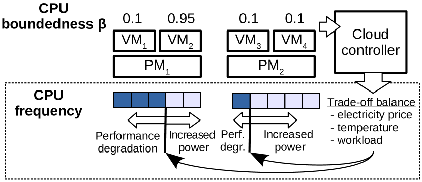
Figure 1: Motivational example.

To illustrate the problem, we provide a motivational example in Fig. 1 with two PM s hosting VM s with different CPU-boundedness properties. The workload consisting of VM s with their $\beta$ values is given as input to the cloud controller, which determines the CPU frequency scaling actions to apply to the PM s as the output. The first machine, $PM_{1}$, hosts $VM_{1}$ with low CPU-boundedness and $VM_{2}$ with high CPU-boundedness, while the second physical machine, $PM_{2}$, hosts $VM_{3}$ and $VM_{4}$, both with low CPU-boundedness. If the cloud operates all hosts at a maximum frequency, the allocated VM s receive good performance, however an increased power consumption may lead to power wastage for VM s 1, 3 and 4 that are not CPU-bound. In order to reduce power consumption, the operating frequencies of the hosts could be adjusted to a minimum frequency. Although this scenario leads to energy savings, it also leads to performance degradation of the CPU-bound $VM_{2}$.

A desirable strategy would be to analyse the trade-offs between energy savings and performance to adaptively select an optimal frequency for each PM independently as shown in Fig. 1. The balance between the two goals depends on many factors such as the workload characteristics, electricity prices and temperatures which all have to be taken into account to determine the optimal frequency. In this ideal scenario, the operating frequencies of PM s hosting VM s with low CPU-boundedness are reduced, e.g. in the case of $PM_{2}$. On the other hand, PM s hosting more CPU-bound VM s are kept high, e.g. in the case of $PM_{1}$, which is set to operate at a high-enough frequency to avoid performance degradation for $VM_{2}$.

The goal of our work is to develop such an adaptive approach that takes into account the CPU-boundedness properties of VM s to achieve energy cost savings without significantly reducing the performance.  The challenges in achieving this goal are: (1) It is necessary to quantitatively determine the balance between energy savings and workload performance to find the optimal CPU frequency. (2) When considering geotemporal inputs, changes in electricity prices and temperatures impact the energy cost and it is necessary to reevaluate the control actions at runtime. To address these challenges, in the next section we present models that allow the comparison of energy savings based on geotemporal inputs and the performance impact quantified as revenue losses caused by frequency scaling in performance-based pricing.

IV Cost-related Components

In this section we define the power and service revenue models that influence cloud costs based on energy consumption and user costs based on VM prices. These two models are used to formulate the trade-off problem and to determine the actions to be deployed by the cloud controller.

IV-A Cloud Cost Model

Power consumption is modelled based on frequency scaling and CPU utilisation using disparate models. The idea is that power consumption of a PM increases with higher resource utilisation caused from more VM s per IaaS cloud models and with higher operating CPU frequencies per high-performance computing (HPC) models. A cubic model based on [25] is used to compute the power consumed when the host is fully utilised according to the operating frequency, $f$. The peak power of the host operating at frequency $f$ is given as:

$$P_{{peak}_{f}}=P_{base}+P_{dif}(\frac{f-f_{base}}{f_{base}})^{3},$$ (1)

where $P_{base}$ is the peak power of the host operating at a minimum frequency $f_{base}$ and $P_{dif}$ is a weight to compute the power at different frequencies. By combining the model from [15] for PM power under a certain utilisation $util$ with Eq. 1, we can express an integrated power model as:  

$$P_{f}=P_{idle}+util(P_{{peak}_{f}}-P_{idle})$$ (2)

where $P_{idle}$ is the power consumed by the PM when hosting no VM s. We compute $util$ as a uniformly weighted fraction of the PM’s CPU cores and RAM consumed by the hosted VM s, as CPU and RAM are shown to be the main contributors of power consumption [26, 27]. The power model graph is shown in Fig. 2 with PM’s power depending on $util$ and CPU frequency. We can see that power decreases significantly for even a small reduction of frequency for high PM utilisation, due to the cubic shape of the curve. Gradually, the curve becomes less steep for lower utilisation ratios. Power consumption of empty PM s is considered to be zero, which is approximately possible through fast suspension technology [24].

Cooling overhead based on local temperatures is derived from the power signals of the PM s at different data center locations. To do so, the model for computer room air conditioning using outside air economisers from [7] was applied. These power signals are then integrated over time and combined with fixed or real-time electricity prices (both models are explored in the evaluation) for the corresponding data center locations to compute the total energy cost of the whole cloud.

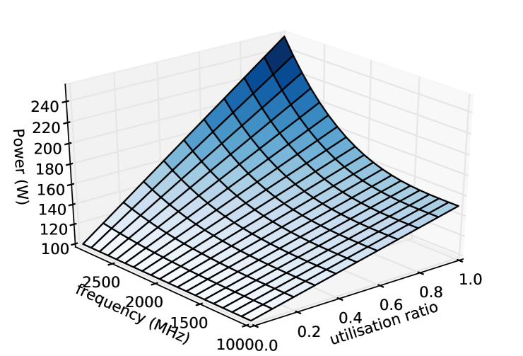
Figure 2: Power model.

IV-B User Cost Model

In performance-based pricing, each VM is charged according to the operating frequency of the PM it is mapped to. The model is based on the pricing offered by the ElasticHosts cloud provider [4]. The price $C_{vm}$ of each VM at frequency $f_{CPU}$ is computed as:

$$C_{vm}=C_{base}+C_{CPU}(\frac{f_{CPU}-f_{base}}{f_{base}})+C_{RAM}(\frac{RAMsize}{RAMsize_{base}}),$$ (3)

where $C_{base}$ is the VM price at a minimum CPU frequency ($f_{base}$) and RAM size ($RAMsize_{base}$). $C_{CPU}$ and $C_{RAM}$ are cost weights used to generate the price from the host’s CPU frequency $f_{CPU}$ and VM RAM size $RAMsize$, respectively.

Given that the above pricing model does not consider how the PM’s CPU frequency affects the VM’s performance (as discussed in Section III), we propose a novel perceived-performance pricing model. In this model, a VM’s price is computed based on both the CPU frequency and its impact on workload performance. The idea is that the price may vary between VM s where CPU frequency impacts the performance at different degrees. E.g., CPU-bound VM s whose performance would be affected by frequency scaling would incur lower monetary costs for the user at a lower frequency than I/O-bound VM s. The impact of frequency scaling on workload performance depends on the CPU-boundedness of the job, represented by the parameter $\beta$ [9]. The pricing model from Eq. 3 is modified to adjust $f_{CPU}$ to be the frequency perceived by the VM computed from the PM’s operating frequency $f$, instead of being the PM’s CPU frequency directly. We model the perceived frequency $f_{CPU}$ as:  

$$f_{CPU}=\beta f+(1-\beta)f_{max},$$ (4)

where $f_{max}$ is the maximum operating frequency of the host. When a VM is CPU-bound, $\beta$ is close to 1 and $f_{CPU}$ changes according to the PM’s operating frequency. As a result, the price charged at a lower frequency is also lower, as the user may perceive significant performance degradation. On the other hand, when $\beta$ is close to 0, which corresponds to the scenario of less CPU-bound VM s where frequency reduction does not impact performance significantly, $f_{CPU}$ is close to $f_{max}$ and the charged price is less dependent on the PM’s operating frequency. A plot of the developed pricing model is shown in Fig. 3. The axes show the host’s operating frequency, the VM’s CPU boundedness $\beta$ and the resulting VM hourly price based on Eq. 4. We can see that VM prices are linearly reduced as a high $\beta$ and a low CPU frequency are approached.

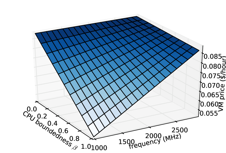
Figure 3: Pricing model.

V Cloud Controller with Frequency Scaling

With the power and pricing models that allow quantitative comparison of energy saving and revenue loss trade-offs, the next step in addressing the problem from Section III is devising the cloud controller algorithm. In this section we present the BCFFS cloud controller we developed for VM migrations and frequency scaling that increases energy cost savings, as long as they exceed service revenue losses. The controller is invoked periodically, determining the actions to be applied. In a production cloud system, the cloud controller would be invoked when new VM requests arrive or geotemporal inputs change for a certain threshold, e.g. temperature changes by over 1 C. Since the two actions of migrating VM s and scaling PM CPU frequencies are mutually orthogonal, we examine them separately as two stages of the proposed algorithm. In the first stage the controller migrates VM s to PM s to maximise utilisation and preferring locations with lower electricity and cooling costs. In the second stage, the controller iteratively reduces CPU frequencies of hosts while the resulting energy savings exceed revenue losses.

V-A VM Migration Stage

The first stage is an algorithm that places new VM s or reallocates VM s from underutilised hosts through VM migration considering power overhead and geotemporal inputs to select hosts. Bin packing of VM s is an NP-hard problem, so we propose a heuristic polynomial time algorithm.

The pseudo-code for this stage of the controller is listed in Alg. 1. The algorithm starts by marking for allocation all newly requested VM s (line 4) and for reallocation all VM s from underutilised hosts (line 5). Hosts are defined as underutilised if their utilisation falls bellow a provider-defined threshold, as discussed in [28]. The VM s marked for allocation will then be migrated (or initially placed) in the outermost loop (line 7) starting with larger VM s first, as they are more difficult to fit (line 6). Available PM s are split into $active$ and $nonactive$ lists, depending on whether they are suspended or not. We sort $inactive$ (line 10) so that larger PM s come first for activation (preferable to more smaller machines, due to the idle power overhead) and data centers with lower combined electricity price and cooling overhead cost are preferred. The target PM to host $vm$ is selected in the inner loop (line 12) by sorting $active$ to try and utilise almost full PM s first, then preferring lower-cost location in case of ties (line 13) and finally activating the next PM from $inactive$ in case $vm$ does not fit on any of the $active$ PM s (line 21). PM sorting is the key step of the algorithm, as it assures that data centers will be filled out based on geotemporal inputs. When a fitting PM is found, the VM is placed or migrated to it (line 24) and the algorithm continues with the next VM.

Algorithm 1 VM Migration Stage.

1:Allocate or migrate VM s per geotemporal inputs.

2:procedure VM Migration Stage

3:    $to\_alloc\leftarrow$ empty list

4:    append all VM s newly requested to $to\_alloc$

5:    append VM s from all underutilised PM s to $to\_alloc$

6:    sort $to\_alloc$ by resource requirements decreasing

7:    for $vm\in to\_alloc$ do

8:       $active\leftarrow$ all PMs where at least one VM is allocated

9:       $inactive\leftarrow$ all PMs where no VMs are allocated

10:       sort $inactive$ by capacity decreasing, cost increasing 

11:       $mapped\leftarrow False$

12:       while not $mapped$ do

13:          sort $active$ by capacity decreasing, cost increasing

14:          for $pm\in active$ do

15:             if $vm$ fits $pm$ then

16:                $mapped\leftarrow True$

17:                break loop

18:             end if

19:          end for

20:          if not $mapped$ then

21:             pop $inactive[0]$ and append it to $active$

22:          end if

23:       end while

24:       perform a placement/migration of $vm$ to $pm$

25:    end for

26:end procedure

V-B Frequency Scaling Stage

After determining the actions to be deployed in the initial stage, the algorithm deploys frequency scaling actions when they lead to energy cost savings that exceed revenue losses based on perceived-performance pricing. The polynomial time algorithm is described in Alg. 2. First, the algorithm resets the frequencies of all the PM s to a maximum frequency $f_{max}$ (line 4). Actions do not have to be executed physically until the procedure halts and the final PM frequencies are determined. Next, the algorithm iterates through the PM s in the outer loop (line 5) to find the best CPU frequency for each one. The algorithm then iteratively scales down the selected frequency according to the range of available CPU frequencies (line 10).

The examined CPU frequency is evaluated based on the following steps: The service revenue from the VM s hosted by the current PM and the energy cost of the PM are computed for the previous and the new frequency (lines 11–12) based on the power and pricing models presented in Section IV. If switching to a new frequency would result in energy cost savings higher than the subsequent revenue loss (line 15), the new frequency is selected (line 19) and the algorithm continues onto the next lower frequency (line 10). The inner loop continues until revenue losses surpass energy savings (line 21). If no frequency decrease occurred for the current PM ($decrease\_feasible$ stays $False$), the procedure will remove PM s with higher average $\beta$ and lower electricity price and temperature in line 27 before continuing. The idea is that such PM s would have even lower energy savings and higher revenue losses, so it is not necessary to consider them.

Algorithm 2 Frequency Scaling Stage.

1:Reduce CPU frequencies while energy savings exceed revenue losses.

2:procedure Frequency Scaling Stage

3:    $decrease\_feasible\leftarrow False$

4:    reset frequency of $\forall pm\in active$ to $f_{max}$ 

5:    for $pm\in active$ do

6:       $f\leftarrow f_{max}$  $\triangleright$ Start the loop at max frequency

7:       $revenue\_cur\leftarrow get\_revenue(pm,f_{to\_apply})$ $\triangleright$ Service revenue, $\forall vm\in pm$

8:       $en\_cost\_cur\leftarrow get\_en\_cost(pm,f_{to\_apply})$$\triangleright$ Energy cost of the $pm$

9:       while $f>f_{min}$ do

10:          $f\leftarrow f-f_{step}$  

11:          $revenue\_new\leftarrow get\_revenue(pm,f)$  $\triangleright$ Revenue for the new frequency  

12:          $en\_cost\_new\leftarrow get\_en\_cost(pm,f)$  $\triangleright$ New energy cost  

13:          $revenue\_loss\leftarrow revenue\_cur-revenue\_new$  

14:          $en\_savings\leftarrow en\_cost\_cur-en\_cost\_new$  

15:          if $en\_savings>revenue\_loss$ then  

16:             $revenue\_cur\leftarrow revenue\_new$  $\triangleright$ Update current service revenue

17:             $en\_cost\_cur\leftarrow en\_cost\_new$  $\triangleright$ Update current energy cost

18:             $decrease\_feasible\leftarrow True$  

19:             $f_{to\_apply}\leftarrow f$  $\triangleright$ Update currently selected frequency  

20:          else

21:             break

22:          end if

23:       end while

24:       if $decrease\_feasible$ then  

25:          apply $f_{to\_apply}$ to $pm$

26:       else

27:          remove from $active$: $\forall\hat{pm}\in PMs$ s.t. $\hat{pm}$ has higher $average(\beta_{vm})$ and lower electricity price and temperature than $pm$  

28:       end if

29:    end for

30:end procedure

VI Evaluation

We evaluated the BCFFS method in a large-scale simulation of 2k VM s based on real traces of geotemporal inputs and VM CPU-boundedness values. The goal of the evaluation is to show the cost savings attainable using our approach, the impact on service revenue and to analyse the dependence on external factors, such as electricity prices and VM workloads.

VI-A Methodology

TABLE I: Simulation parameters.

PM s	VM s	$f_{base}$	$f_{min}$	$f_{max}$	$f_{step}$	$P_{base}$	$P_{idle}$	$P_{dif}$	$C_{base}$	$C_{CPU}$	$C_{RAM}$	$RAMsize_{base}$
2k	2k	1 GHz	1.8 GHz	2.6 GHz	200 MHz	150 W	100 W	15 W	0.027 $/h	0.018 $/h	0.025 $/h	1 GB

The simulations were performed using Philharmonic, a cloud controller simulator for geographically-distributed clouds that we developed [16]. A simulation in Philharmonic consists of iterating through the timeline, collecting the currently available electricity prices and temperatures, as well as the incoming VM requests. The simulated controller is called to determine cloud control actions, such as VM migrations or PM frequency scaling. The applied actions are used to compute the resulting energy consumption and electricity costs.

To compute the energy costs of the simulated geographically-distributed cloud, we consider a use case of six data centers. We used a dataset of real-time electricity prices described in [17] and temperatures from the Forecast web service. The selected data center locations (chosen to resemble Google’s deployment) are shown in Fig. 4. Due to lack of RTEP data for the four non-US cities, we synthetically generated electricity prices from the data known for other US cities. We shifted the time series based on the time zone offsets and added a difference in annual mean values to resemble local values. Additionally, in the evaluation we analyse a scenario with fixed electricity prices, where mean values constant over time are considered for each location.

Figure 4: Cities used as data center locations in the simulation.

To generate realistic VM CPU-boundedness values, we analysed the PlanetLab dataset of CPU usage traces for 1024 VM s collected every five minutes throughout a day. We mapped each VM’s average CPU usage to a $\beta$ value. From the generated $\beta$ dataset, we fit an exponential distribution, shown in Fig. 5. The empirical histogram of the traces normalised to an area of 1 is also included. We used this model to generate the $\beta$ values of the VM s in the simulation.

We consider the perceived-performance pricing model from Section IV. We also evaluated the ElasticHosts performance-based pricing model, but CPU frequency scaling was not feasible, due to high VM prices compared to energy costs. Savings are still possible with our perceived-performance pricing model, as for certain less CPU-bound VM workloads a CPU frequency reduction does not decrease the service revenue substantially and yet achieves energy savings.

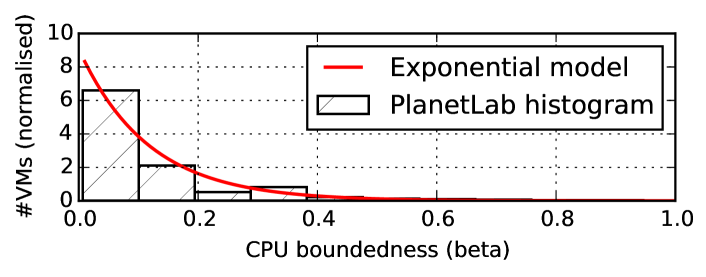
Figure 5: VM CPU-boundedness distribution from PlanetLab traces.

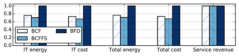
Figure 6: Aggregated results for a 2k VM simulation using different controllers.

The parameters used in the simulation are summarised in Table I. To define the cloud, the number of total $PMs$ and $VMs$ for the case of VM boot requests is given. The resource values we assumed in this simulation (number of CPU cores, amount of RAM) were uniformly distributed. For each VM, we used one CPU core and ranged the amount of RAM between 8-32 GB to vary resource utilisation over time and VM price depending on RAM size. PM s were varied between 1-4 CPU cores and 16-32 GB RAM, to model a heterogeneous infrastructure. The boot time and duration of the VM requests were randomly generated following a uniform distribution within the simulation time to vary the duration of the VMs and distribute delete events. The total duration of the simulation was set to 168 h (7 days), with 1 h step size. The simulation step size was selected based on the available geotemporal input datasets, but the cloud controller could be invoked at different periods in production cloud systems (e.g. on new VM requests or geotemporal input changes). Based on the workload and PM capacity, at most 1k PM s were active at once. Each PM can operate in five frequency modes between a minimum and maximum frequency, $f_{min}$ and $f_{max}$ respectively, in steps of 200 MHz ($f_{step}$), similar to [25]. To define the cost models, the parameters used for the power model in Eq.1 were based on [25] and the idle power, $P_{idle}$, was assumed to be equal to 50% of the peak value (at maximum frequency), $P_{peak_{f_{max}}}$, like in [29]. The parameters for the pricing model of Eq. 3 were based on the hourly ElasticHosts [4] VM prices. We also assume the cost of other resources, e.g. disk, that are not used in this study to be fixed. The specified settings were used in all the experiments, unless otherwise stated (e.g. when certain parameters were varied to measure their impact).

We consider two baseline controllers for results comparison. The first controller is a method for VM migration dynamically adapting to user requests using a best fit decreasing (BFD) placement heuristic developed in [12]. The second baseline controller we developed called best cost fit (BCF) is a variant of the BCFFS controller that applies VM migration based on geotemporal inputs, but no frequency scaling. As the focus of this work is on frequency scaling under performance-based pricing, the BCF baseline method allows us to quantify the improvement brought by this specific aspect.

In the remainder of the section we show the results for different scenarios to compare the energy savings and revenue loss resulting from applying our cloud controller approach.

VI-B Energy Costs and Service Revenue

TABLE II: Absolute aggregated simulation results

	BCF	BCFFS	BFD
IT energy (kWh)	16226.87	15028.00	21261.16
IT cost ($)	735.29	674.14	1002.19
Total energy (kWh)	19477.54	18043.00	25443.02
Total cost ($)	878.80	805.86	1193.82
Service revenue ($)	62995.63	62977.79	62995.63

We start the analysis of the results with the aggregated energy costs and service revenue of the proposed method and the considered baseline methods for the 2k-VM simulation described in Table I. The aggregated results are shown in Fig. 6. A column group is shown for each of the examined metrics – energy and cost used by the IT equipment, total energy and cost that also include the cooling overhead based on outside temperatures and the service revenue obtained from hosting the VM s based on the perceived-performance pricing model. In each group, there is a column for our proposed BCFFS controller and the two baseline methods. The values are normalised as a relative value of the BFD baseline controller’s results. Absolute values are listed in Table II. The proposed BCFFS controller achieves $32\%$ total energy cost savings compared to the BFD controller and $8\%$ compared to the BCF controller. No significant service revenue losses are incurred by BCFFS. Based on our perceived-performance pricing model, this also indicates no significant performance degradation. Since similar service revenue and performance results were obtained for other simulations as well, we omit the results for service revenue losses in the rest of the section.

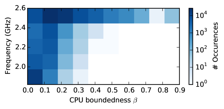
Figure 7: Occurrences of $(\beta,f)$ combinations among the controlled VM s.

To explore the frequencies $f$ assigned to VM s in the simulation and compare them with the VM s’ CPU boundedness $\beta$, we counted the number of occurrences of each $(\beta,f)$ combination for every VM and time slot. This data is illustrated as a bivariate histogram in Fig. 7 with the number of occurrences shown on a logarithmic scale. Darker areas show a higher number of frequency occurrences for the respective $(\beta,f)$ combination. It can be seen that the occurrences of CPU frequencies assigned based on each VM’s CPU boundedness match the areas where VM prices are high based on the pricing model from Fig. 3. The area with high $\beta$ and low $f$, where prices would be the lowest, contains no occurrences. The darkest areas of the graph with a high number of occurrences represent the balance between energy savings and profit losses, which is in line with the controller requirements that energy cost savings should be maximised, but not exceeded by revenue losses.

VI-C Cloud size variation

We simulated clouds with different numbers of hosts and a proportional frequency of incoming VM requests to examine the energy cost savings at different scales. The number of hosts was ranged from 200 to 1.2k with a step size of 200. The incoming requests were generated proportionally to the number of hosts to keep the utilisation fixed. In Fig. 8, we show the results in terms of absolute energy costs. We can see that the absolute energy costs savings increase for a larger number of hosts, as the cost of operating the hosts increases. However, the performance of the algorithm is not greatly affected by the number of hosts, achieving similar relative energy cost savings in all the cases.

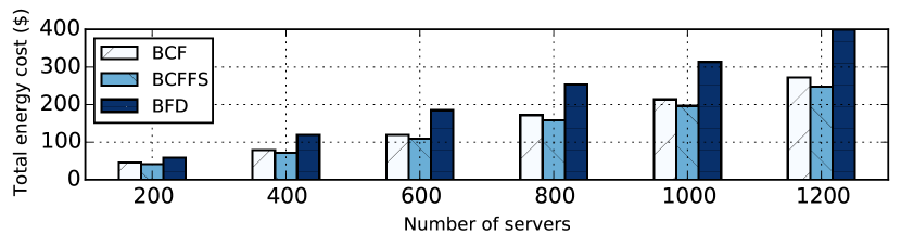
Figure 8: Energy cost savings for different number of hosts and VM s.

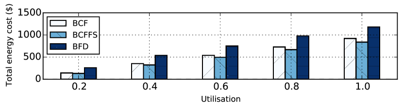
Figure 9: Energy cost savings for different cloud utilisation rates.

VI-D Utilisation Variation

To investigate the performance of the algorithm in terms of energy savings and revenue loss for different utilisation scenarios, we vary the number of VM requests for the same number of PM s. Energy costs from frequency scaling and revenue loss of the BCFFS controller compared to the BCF controller for different utilisation scenarios are shown in Fig. 9. Although no significant revenue loss occurs for any of the scenarios, energy savings using frequency scaling increase as cloud utilisation increases. This is due to the concave shape of the power model, where power decreases faster with CPU frequency reduction for higher utilisation. The BCFFS controller is therefore best suited for highly utilised PM s.

VI-E Electricity Cost Variation

Different cloud providers can have access to different electricity pricing schemes. Although some might have access to RTEP, it is also interesting to see how our controller would perform under fixed electricity pricing. In this set of experiments, we compare scenarios for fixed and variable electricity prices to investigate the impact of electricity pricing on the energy savings attainable using the BCFFS algorithm. The results are shown in Fig. 10. Energy costs are reduced under variable electricity pricing by exploiting runtime information and adapting the cloud configuration within the day according to electricity price changes. In both cases, however, the proposed cloud controller, BCFFS, achieves significant savings compared with the baseline algorithms.

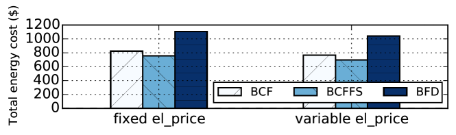
Figure 10: Energy cost savings for fixed and variable electricity pricing options.

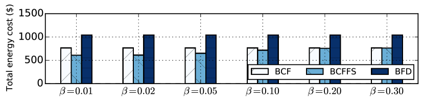
Figure 11: Energy cost savings for VM s with different fixed CPU-boundedness.

VI-F CPU-Boundedness Variation

To evaluate the impact of different workloads, we ran simulations using the same PM s and VM requests with only the VM CPU-boundedness properties being varied. We generated scenarios with VM s of fixed CPU-boundedness properties and evaluated the total energy cost of the cloud controllers for each scenario. The total energy costs for CPU-boundedness properties ranging from $0.01$ to $0.3$ are shown in Fig. 11. With the increase of CPU-boundedness $\beta$, energy costs of the BCFFS controller increase gradually. Between a $\beta$ of $0.05$ and $0.2$ there is a substantial energy cost increase. This happens when the revenue losses exceed energy cost savings from even an initial frequency reduction and at this point no frequency scaling is performed. The BCFFS controller achieves the best results for predominantly I/O-bound workloads.

VII Conclusion

In this paper we proposed a novel perceived-performance pricing model that would enable applying energy saving actions on VM s where CPU frequency scaling would not degrade the performance. We presented a cloud controller that utilises said pricing model and applies VM migrations and CPU frequency scaling accounting for the trade-offs of service revenue losses and energy cost savings in a geographically-distributed cloud. We evaluated the proposed cloud controller in a simulation using realistic CPU-boundedness data, electricity prices and temperatures. Our results show significant energy cost savings can be achieved without reducing service revenue. Also, we highlighted parameters that improve the controller’s efficiency, such as low workload CPU-boundedness and high PM utilisation, that can help cloud providers assess the method’s potential applicability. In the future we plan to improve the research with memory power management and a more detailed power model for frequency scaling on multiple cores. This will allow us to more precisely estimate the controller’s efficiency for a wider range of VM instance types.

References

- [1] W. Felter, A. Ferreira, R. Rajamony, and J. Rubio, “An Updated Performance Comparison of Virtual Machines and Linux Containers,” IBM Research Division, Technology, vol. 28, p. 32, 2014.
- [2] J. O’Loughlin and L. Gillam, “Performance Evaluation for Cost-Efficient Public Infrastructure Cloud Use,” in Economics of Grids, Clouds, Systems, and Services. Springer, 2014, pp. 133–145.
- [3] I. Pietri and R. Sakellariou, “Cost-efficient provisioning of cloud resources priced by CPU frequency,” in Proceedings of the 7th IEEE/ACM International Conference on Utility and Cloud Computing (UCC). IEEE, 2014, pp. 483–484.
- [4] ElasticHosts, Available:http://www.elastichosts.co.uk/.
- [5] Jonathan Koomey, “Growth in Data center electricity use 2005 to 2010,” Analytics Press, Oakland, CA, Tech. Rep., Aug. 2011. [Online]. Available: http://www.analyticspress.com/datacenters.html
- [6] R. Weron, Modeling and Forecasting Electricity Loads and Prices: A Statistical Approach, 1st ed. Wiley, Dec. 2006.
- [7] H. Xu, C. Feng, and B. Li, “Temperature aware workload management in geo-distributed datacenters,” in Proceedings of the ACM SIGMETRICS/international conference on Measurement and modeling of computer systems, vol. 41. ACM, 2013, pp. 373–374.
- [8] A. Miyoshi, C. Lefurgy, E. Van Hensbergen, R. Rajamony, and R. Rajkumar, “Critical power slope: understanding the runtime effects of frequency scaling,” in Proceedings of the 16th International Conference on Supercomputing (ICS). ACM, 2002, pp. 35–44.
- [9] V. W. Freeh, D. K. Lowenthal, F. Pan, N. Kappiah, R. Springer, B. L. Rountree, and M. E. Femal, “Analyzing the energy-time trade-off in high-performance computing applications,” IEEE Transactions on Parallel and Distributed Systems (TPDS), vol. 18, no. 6, pp. 835–848, 2007.
- [10] G. Von Laszewski, L. Wang, A. J. Younge, and X. He, “Power-aware scheduling of virtual machines in DVFS-enabled clusters,” in Proceedings of the IEEE International Conference on Cluster Computing and Workshops (CLUSTER). IEEE, 2009, pp. 1–10.
- [11] W. Shi and B. Hong, “Towards profitable virtual machine placement in the data center,” in Proceedings of the 4th IEEE International Conference on Utility and Cloud Computing. IEEE, 2011, pp. 138–145.
- [12] A. Beloglazov, J. Abawajy, and R. Buyya, “Energy-aware resource allocation heuristics for efficient management of data centers for Cloud computing,” Future Generation Computer Systems, vol. 28, no. 5, pp. 755–768, May 2012.
- [13] C.-M. Wu, R.-S. Chang, and H.-Y. Chan, “A green energy-efficient scheduling algorithm using the DVFS technique for cloud datacenters,” Future Generation Computer Systems (FGCS), vol. 37, pp. 141–147, 2014.
- [14] H. Guler, B. Cambazoglu, and O. Ozkasap, “Cutting Down the Energy Cost of Geographically Distributed Cloud Data Centers,” in Energy Efficiency in Large Scale Distributed Systems. Vienna: Springer Berlin Heidelberg, 2013, pp. 279–286.
- [15] Z. Liu, Y. Chen, C. Bash, A. Wierman, D. Gmach, Z. Wang, M. Marwah, and C. Hyser, “Renewable and cooling aware workload management for sustainable data centers,” in Proceedings of the 12th ACM SIGMETRICS/PERFORMANCE joint international conference on Measurement and Modeling of Computer Systems, ser. SIGMETRICS ’12. New York, NY, USA: ACM, 2012, pp. 175–186.
- [16] D. Lučanin, F. Jrad, I. Brandic, and A. Streit, “Energy-aware cloud management through progressive SLA specification,” in 11th International Conference on Economics of Grids, Clouds, Systems, and Services (GECON). Springer, 2014, pp. 83–98.
- [17] S. Alfeld, C. Barford, and P. Barford, “Toward an analytic framework for the electrical power grid,” in Proceedings of the 3rd International Conference on Future Energy Systems: Where Energy, Computing and Communication Meet, ser. e-Energy ’12. New York, NY, USA: ACM, 2012, pp. 9:1–9:4.
- [18] A. Qureshi, R. Weber, H. Balakrishnan, J. Guttag, and B. Maggs, “Cutting the electric bill for internet-scale systems,” SIGCOMM Comput. Commun. Rev., vol. 39, no. 4, pp. 123–134, Aug. 2009.
- [19] N. Buchbinder, N. Jain, and I. Menache, “Online Job-Migration for Reducing the Electricity Bill in the Cloud,” in NETWORKING 2011, ser. Lecture Notes in Computer Science, J. Domingo-Pascual, P. Manzoni, S. Palazzo, A. Pont, and C. Scoglio, Eds. Springer Berlin Heidelberg, Jan. 2011, no. 6640, pp. 172–185.
- [20] M. Etinski, J. Corbalan, J. Labarta, and M. Valero, “Optimizing job performance under a given power constraint in HPC centers,” in Proceedings of the International Green Computing Conference (IGCC), 2010, pp. 257–267.
- [21] C.-H. Hsu and U. Kremer, “The design, implementation, and evaluation of a compiler algorithm for CPU energy reduction,” ACM SIGPLAN Notices, vol. 38, no. 5, pp. 38–48, 2003.
- [22] T. Mastelic, J. Jasarevic, and I. Brandic, “A novel performance metric based on real-time cpu resource provisioning in time-shared cloud environments,” in 6th IEEE International Conference on Cloud Computing Technology and Science. IEEE, 2014, pp. 408–415.
- [23] H. Liu, C.-Z. Xu, H. Jin, J. Gong, and X. Liao, “Performance and energy modeling for live migration of virtual machines,” in Proceedings of the 20th international symposium on High performance distributed computing, 2011, pp. 171–182.
- [24] D. Meisner, B. T. Gold, and T. F. Wenisch, “PowerNap: eliminating server idle power,” SIGPLAN Not., vol. 44, no. 3, pp. 205–216, Mar. 2009.
- [25] J.-M. Pierson and H. Casanova, “On the utility of DVFS for power-aware job placement in clusters,” in Proceedings of Euro-Par. Springer, 2011, pp. 255–266.
- [26] R. Basmadjian, N. Ali, F. Niedermeier, H. de Meer, and G. Giuliani, “A methodology to predict the power consumption of servers in data centres,” in Proceedings of the 2nd International Conference on Energy-efficient Computing and Networking (e-Energy). ACM, 2011, pp. 1–10.
- [27] A. Kansal, F. Zhao, J. Liu, N. Kothari, and A. A. Bhattacharya, “Virtual machine power metering and provisioning,” in Proceedings of the 1st ACM Symposium on Cloud Computing (SoCC). ACM, 2010, pp. 39–50.
- [28] A. Beloglazov and R. Buyya, “Managing Overloaded Hosts for Dynamic Consolidation of Virtual Machines in Cloud Data Centers Under Quality of Service Constraints,” IEEE Transactions on Parallel and Distributed Systems, vol. 24, no. 7, pp. 1366–1379, 2013.
- [29] X. Fan, W.-D. Weber, and L. A. Barroso, “Power provisioning for a warehouse-sized computer,” in ACM SIGARCH Computer Architecture News, vol. 35, no. 2. ACM, 2007, pp. 13–23.