Pervasive Cloud Controller for
Geotemporal Inputs

Abstract

The rapid cloud computing growth has turned data center energy consumption into a global problem. At the same time, modern cloud providers operate multiple geographically-distributed data centers. Distributed data center infrastructure changes the rules of cloud control, as energy costs depend on current regional electricity prices and temperatures. Furthermore, to account for emerging technologies surrounding the cloud ecosystem, a maintainable control solution needs to be forward-compatible. Existing cloud controllers are focused on virtual machine (VM) consolidation methods suitable only for a single data center or consider migration just in case of workload peaks, not accounting for all the aspects of geographically distributed data centers. In this paper, we propose a pervasive cloud controller for dynamic resource reallocation adapting to volatile time- and location-dependent factors,  while considering the QoS impact of too frequent migrations and the data quality limits of time series forecasting methods. The controller is designed with extensible decision support components. We evaluate it in a simulation using historical traces of electricity prices and temperatures. By optimising for these additional factors, we estimate $28.6\%$ energy cost savings compared to baseline dynamic VM consolidation. We provide a range of guidelines for cloud providers, showing the environment conditions necessary to achieve significant cost savings and we validate the controller’s extensibility. 

1 Introduction

To satisfy growing cloud computing demands, data centers are consuming more and more energy, accounting for 1.5% of global electricity usage [1] and annual electricity bills of over $40M for large cloud providers [2]. At the same time, a trend of more geographically distributed data centers can also be seen, e.g. Google has twelve data centers across four continents. As new paradigms develop, such as smart buildings with integrated data centers [3], computation is shaping as a distributed utility. Such cloud deployments result in dynamically changing energy cost conditions and require new approaches to cloud control.

Assorted technological innovations have brought forth the optimisation of several independent systems that affect cloud operation, creating a heterogeneous and dynamically variable environment. The technologies of the next-generation electricity grid known as the “smart grid”, distributed power generation, microgrids and deregulated electricity markets have lead to demand response and real-time electricity pricing (RTEP) options where prices change hourly or even minutely [4, 5]. Additionally, new solutions for cooling data centers (an energy overhead reported to range from 15% to 45% of a data center’s power consumption [6]) based on outside air economizer technology result in cooling efficiency depending on local weather conditions. We call such time- and location-dependent factors geotemporal inputs. Geotemporal inputs may also include renewable energy availability [7], peak load electricity pricing [8] or demand response [9, 10] as they constitute time- and location-dependent factors that impact the final energy costs as well.

Furthermore, as IT-based optimisation solutions enter more and more domains, we may expect the emergence of new geotemporal inputs in the future. Examples include more options for precisely calibrating electricity usage and pricing in smart grids, local renewable energy generation, further geographical distribution and bringing data centers closer to users through smart buildings [3] and all in all more advanced metering infrastructure for quantifying cloud service demand and usage through smart cities, smart homes, mobile technology or more generally the Internet of Things (IoT). We denote geotemporal inputs, cloud requirements, regulations and other factors that guide the cloud provider’s actions as decision support components. We define forward compatiblility as being able to cope with additional decision support components without drastic changes of the core architecture. Hence, to account for cloud environment evolution, a forward-compatible cloud controller is necessary where the decision support components are extensible with yet-to-be-realised geotemporal inputs and other factors.

Cloud control approaches can be classified into three levels: (1) The first level consists only of initial VM placement when the user requests it. For this class of algorithms, existing solutions from the field of grid computing [11] or network request routing [2] can be applied, where geotemporal inputs are used to determine the best placement target. Once placed, however, the VM, job or network request is never moved. (2) The second level is dynamic VM consolidation to apply live VM  migrations and optimally reallocate active VM s after requests to boot new or delete existing VM s arrive. Existing cloud controllers that apply VM reallocation [12, 13, 14] are focused on a model suitable for a single data center, where no energy heterogeneity inherent to geotemporal inputs is considered. (3) The third level, what we call pervasive control, is controlling the cloud’s resource allocation dynamically to both consolidate resources and adapt to volatile geotemporal inputs by utilising more cost-efficient data centers through long-term planning facilitated by forecasting and the asserted data quality. The challenges of pervasive control of clouds according to multiple decision criteria, including volatile geotemporal inputs are that too frequent VM migrations to reallocate the cloud’s resource consumption cause downtimes [15] which harm the quality of service (QoS). Forecasting of geotemporal inputs is necessary to find the optimal balance between energy cost saving and VM migration overhead trade-offs. With time series forecasting that enables long-term planning, the issue of data quality also has to be considered to account for the forecasting accuracy and reach. Additionally, designing a controller to enable turning off or adding new decision support components is necessary to integrate the solution into diverse cloud deployments and ensure forward compatibility. To the best of our knowledge, no existing cloud control method addresses these challenges. which is the goal of our work. 

In this paper we propose a novel pervasive cloud controller designed for resource allocation optimisation that efficiently utilises cloud infrastructure, accounting for geographical data center distribution under geotemporal inputs. Our model of a forward-compatible optimisation engine supports components for costs based on geotemporal inputs, VM migration overheads, QoS requirements and other inputs to be composed in a unified optimisation problem specification. A schedule of VM migrations is planned ahead of time in a forecast window. This allows the controller to minimise energy costs by planning over a long-term period such as hours or days, while retaining the required QoS, i.e. not incurring too frequent VM migrations. To assess the application of our pervasive cloud controller in diverse cloud deployments, we present a number of guidelines showing how the effectiveness changes under different geotemporal input patterns, geographical distributions and forecast data quality.

As a proof of concept evaluation we present an implementation of the pervasive cloud controller based on a hybrid genetic algorithm for optimising the schedule of VM migrations. A time-series-based schedule representation is developed for integration with geotemporal inputs to facilitate long-term planning. A realistic duration-agnostic model, with no a priori VM lease duration knowledge assumption, improves the compatibility with real cloud deployments, such as Amazon EC2, Google Compute Engine or private OpenStack clouds. Multiple decision support components including energy cost, QoS, migration overhead and capacity constraints are combined into an extensible fitness function, matching the forward compatibility requirements. 

We evaluate the pervasive cloud controller in a large-scale simulation consisting of 10k VM s using historical electricity price and temperature traces to show the resulting energy cost savings and QoS impact. Based on our simulation results, energy cost savings can be increased up to $28.6\%$ compared to a baseline scheduling algorithm [16] with dynamic VM consolidation. Furthermore, we expand the evaluation to provide guidelines for cloud providers in terms of how different geotemporal input value ranges and geographical data center distributions affect the method’s effectiveness. We provide a data quality analysis by evaluating the controller under different forecasting errors. Finally, we validate the architecture’s extensibility by performing the simulation with different subsets of decision support components.

In the remainder of this paper, Section 2 examines the related work. We explain the research problem intuitively on a real example of geotemporal inputs and provide a high-level description of our pervasive cloud controller in Section 3. The formal specification of the plug-and-play decision support components and the optimisation problem specification is presented in Section 4. The proof-of-concept implementation of the forward-compatible optimisation engine of the pervasive cloud controller we developed is explained in Section 5 and in Section 6 we describe the evaluation methodology and discuss the results.

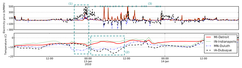
Figure 1: Geotemporal inputs (real-time electricity prices and temperatures) at four locations in the USA during a period of three days – temperature values within a single day change up to 15 degrees between peaks and lows; and even larger relative differences can be observed in the volatile electricity prices. Electricity price data obtained from [17] and temperatures from [18].

2 Related Work

We structure the related work overview using the already mentioned three-level classification of cloud control methods.

Looking at the first level of methods that only perform initial placement and consider geotemporal inputs during host selection, the approach was pioneered by Quereshi et al. [2]. Their work shows the potential of optimising distributed systems (adaptive network routing in content delivery networks) for RTEP, estimating savings up to 40% of the full electricity cost. Similar routing approaches are explored in [19, 20, 21] and considering both electricity prices and $CO_{2}$ emissions in [22]. Initial placement is also researched in the context of map-reduce jobs [23] and based both on RTEP and cooling in computational grids in [24, 25]. A theoretical analysis of placing grid jobs with regards to electricity prices, job queue lengths and server availability is given in [26]. A power-aware job scheduler with no rescheduling and assuming a priori job duration knowledge is presented in [4].

The second level includes methods targeted at modern infrastructure as a service (IaaS) clouds where live VM migration is used to dynamically reallocate resources and reduce energy consumption. These methods, however, value energy the same, no matter the time or location, and therefore overlook the additional challenges and optimisation potential of geotemporal inputs. Feller et al. proposed a distributed scheduling algorithm for dynamic VM consolidation using live migrations, based on hierarchical group management [12]. Beloglazov et al. [13] introduced a VM consolidation method that minimises the migration frequency in an online controller, taking future workload predictions into consideration. A rule-based VM consolidation approach is developed in [14]. Practical cloud control utilising VM migrations with a focus on high scalability in production VMware systems is researched in [27]. Consolidation based on RAM and CPU usage is researched and evaluated on a real data center in [28].

The third level requires pervasive cloud control where VM s are dynamically migrated to adapt both to user requests and changes in geotemporal inputs that enable energy cost savings, while considering forecast data quality and QoS requirements. There have been initial advances in this direction. Cauwer et al. [29] presented a method of applying time series forecasting of electricity prices to detect how a data center’s resource consumption should be controlled in a geographically distributed cloud, but for a simplified model with no concrete actions that should be applied on VM s. Determining exact per-VM actions is a challenging trade-off problem, between closely following volatile geotemporal input changes and minimising the number of migrations to retain high QoS, as we will examine in the following section. Abbasi et al. [30] started researching migrating VM s based on RTEP, but for a limited workload distribution scenario where a physical machine (PM) hosts only a single VM. Additionally, temperature-dependent cooling energy overhead and forecasting errors are not considered. Our work addresses these challenges through a holistic model supporting multiple decision support components and long-term planning facilitated by forecasting and data quality assertion.

Finally, we look at work related to ours from an algorithmic perspective. Approaches for schedule optimisation based on a forecast horizon are explored as rolling-horizon real-time task scheduling in [31] and a genetic algorithm for this purpose was used for multi-airport capacity management with receding horizon control in [32]. A genetic algorithm for optimising energy consumption in computational grids using dynamic voltage & frequency scaling (DVFS) is presented in [33]. Tabu search, a related meta-heuristic optimisation method, is used for static data center location and capacity planning with a focus on network traffic in [34].

3 Geotemporal Cloud Environments

We now explain the geotemporal environment surrounding geographically-distributed clouds on a real example of electricity prices and temperatures. On this use case, we will give an overview of the problem on an intuitive level and give a high-level description of our pervasive cloud controller, before detailing the formal specification of the model in the following section.

3.1 Problem Overview

Example geotemporal inputs for four US cities are shown in Fig. 1. Rapid changes in geotemporal inputs can occur dynamically. The peak that can be seen in Dubuque on January 12th from 21:00 to 23:00 (1), results in five or more times the average prices. It can be observed that temperature peaks occur towards the end of the day, while lows occur during nights. Even though electricity price is more volatile, partial dependence on previous data points can be seen. This means that it is possible to model their behaviour to forecast probable future values, and in fact is done in practice [5, 18].

To explain the potential and challenges of geotemporal inputs in the context of cloud computing, let us assume that there are two data centers – one in Detroit and another one in Dubuque. For the data shown in Fig. 1 during the period (1), it makes sense to run more VM s in Detroit when temperatures are the same, because electricity is more expensive in Dubuque (constantly over 100 $/MWh, reaching 500 $/MWh) than in Detroit (less than 100 $/MWh). However, when it gets 10 C colder in Dubuque three hours later (2) and electricity prices become lower than in Detroit, less energy would be consumed on cooling there, resulting in lower energy costs, so it is better to migrate a number of VM s from Detroit to Dubuque and shift computational load this way.

A challenge in adapting cloud control for geotemporal inputs is that the cloud provider cannot migrate VM s between different locations too rapidly, as this wastes bandwidth, incurs an energy overhead and impacts QoS. This is underlined even more by the volatile variable behaviour observable in electricity prices. In Fig. 1, we marked by crosses (3) all the moments throughout January 13th when ratios between electricity prices in Detroit and Dubuque change significantly, offering an opportunity to save on energy costs by reallocating VM s using live migrations. We can see that 19 migrations would be performed this way. If we assume a downtime caused by a live VM migration to last for one minute, which is possible based on the model presented in [15], this would result in a VM availability of 98.68%. This availability is considerably lower than the 99.95% availability rates advertised by Amazon and Google in their service level agreement (SLA) and incurs extra data transfer costs. The challenges arising from this are: (1) To profit from geotemporal inputs in cloud computing, the trade-offs of the energy savings of geotemporal inputs, the migration overheads and impact on QoS, as well as the data accuracy provided by the forecasting methods for future geotemporal inputs all have to be considered and reconciled in a long-term plan. (2) In reality, the problem has to be solved on a much larger scale with more data centers and thousands of VM s. New ways of controlling VM s across geographically-distributed data centers have to be developed to address these challenges.

3.2 Pervasive Cloud Controller

We now present our pervasive cloud controller approach by explaining the identified requirements, defining the architecture of the solution and giving a high-level overview of its workflow.

3.2.1 Requirements

In our approach, we consider an IaaS cloud provider hosted on multiple geographically distributed data centers. The cloud is assumed to be operating in an environment comprising geotemporal inputs such as RTEP and temperature-dependent cooling efficiency (other inputs can be added as well). The cloud is governed by a controller system that manages virtual and physical machines in all data centers and can issue actions, such as migrating a VM from one PM to another, suspending or resuming a PM.

TABLE I: Example SLA.

#CPUs	RAM	storage	availability	price
4	15 GB	80 GB	$99.95\%$	$0.28/hour

The first input are user goals represented by SLA s, specifying the number of requested VM s, their resource and QoS requirements. An example of user requirements for an Amazon m3.xlarge VM  specified in an SLA is shown in Table I. The second input are the geotemporal inputs, providing time series metrics describing each of the data center locations, such as electricity price and temperature data, example values of which are shown in Fig. 1. Each geotemporal input is a time series of past and current values and, using time series forecasting, it is possible to predict future values and the accompanying data quality (reach and the most likely error rate). The controller’s task is to output a schedule that determines where each VM is deployed and for each PM if it is running or suspended at any point in time.

3.2.2 Architecture

Fig. 2 shows the architecture of our proposed pervasive cloud controller for managing a geographically distributed cloud based on geotemporal inputs. On a high level, geotemporal inputs are used to obtain forecast data and the corresponding quality. This input is, together with the SLA s, provided to the pervasive cloud controller, which generates a long-term schedule of control actions to apply to the geographically distributed data centers.

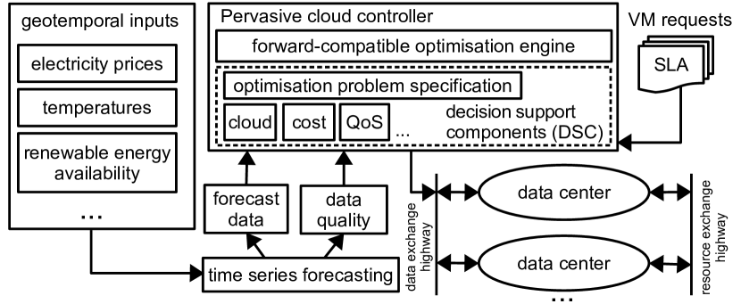
Figure 2: Pervasive cloud controller architecture.

Looking at the architecture details, geotemporal input forecasts are converted by the controller into values meaningful to the cloud provider, e.g. data center energy costs that combine RTEP with the cooling overhead, environmental impact etc. These measures along with other internal measures like cloud capacity and the QoS stemming from actions planned for VM s are all combined into an optimisation problem specification as decision support components. To support new geotemporal inputs, SLA metrics or cloud regulations, it is important for the decision support components to be extensible in a plug-and-play manner, i.e. without requiring architectural changes. We formally present the decision support component model in the following section. The role of ensuring decision support component extensibility lies in a forward-compatible optimisation engine. It considers the decision support components as criteria to plan and optimise a schedule of control actions for a future period. The challenging part of ensuring forward compatibility with new decision support components is that there has to be a separation of the schedule evaluation logic and the optimisation logic. The schedule is evaluated using geotemporal inputs and the time-based allocation of VM s to PM s, to estimate the actions’ outcome in terms of costs, QoS and any other decision support components. This evaluation is then used by the controller in a black-box manner to explore the search space of possible actions using its custom optimisation logic and the high-level information about each schedule returned by the evaluation logic. The selected schedule is applied over time to physical and virtual machines in the cloud (forwarding control actions through a data exchange highway) by utilising live VM migrations as a resource exchange highway to redistribute computational load between the data centers.

3.2.3 Workflow

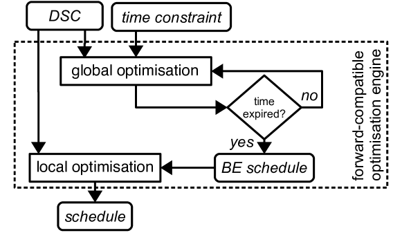
Figure 3: Optimisation engine workflow.

The forward-compatible optimisation engine worfklow is illustrated in Fig. 3. It collects the decision support components, related together as an optimisation problem specification and produces a schedule of control actions to apply in the cloud. Given that bin packing of allocating VM s to PM s is an NP-hard problem and in our case we add to it the dimension of time and time-related QoS requirements (e.g. the VM migration frequency), an optimal solution can not be found at runtime for an arbitrary problem size. To overcome this, we propose a two-stage optimisation process. The first stage is a global optimisation method that sweeps the whole search space looking for a global optimum within a time constraint (provided as an additional parameter that the cloud provider specifies). We then take the best-effort schedule this method was able to find (BE schedule) and pass it to a second stage local optimisation method that continues to improve it with a primary goal of satisfying all the hard constraints among the decision support components that the global optimisation failed to satisfy. In Section 5 we present our proof-of-concept implementation for the global and local optimisation methods based on a hybrid genetic algorithm with greedy local constraint satisfaction. We later use these methods to evaluate the pervasive cloud controller.

4 Decision Support Components

In this section we formally specify the cloud, QoS and cost decision support components and show how they are related together into an optimisation problem specification of optimisation goals and constraints. These decision support components are then used by the optimisation engine in the schedule generation.

4.1 Cloud and QoS Components

We consider a single IaaS cloud provider that is represented by $DCs$, a set of $d$ geographically-distributed data centers and $PMs$, a set of $p$ physical machines it operates. We define each physical machine’s location at one of the data centers.

$$\forall pm\in PMs,\ loc(pm)\in DCs$$ (1)

As we are modelling dynamic system behaviour, we define a time period in the range from $t_{0}$ to $t_{N}$ (denoted $[t_{0},t_{N}]$), of $N$ discrete (arbitrarily small) periods.  

User requirements are defined by $vmreqs_{t}$, a set of virtual machine requests at a moment $t$, each of which can either ask for a new VM  to be booted or an existing one to be deleted. These events are controlled by end users and we assume no prior knowledge of the users’ requests (as is the case in IaaS clouds like Amazon EC2). Based on the past and current $vmreqs_{t}$, we define $VMs_{t}$, a set of VMs provided to the users at time $t$.

The cloud provider defines an extensible set of $r$ resource types that have to be specified through an SLA, e.g. number of CPUs and amount of RAM. The exact resources for a single VM are an ordered $r$-tuple of values, defining the VM’s $spec$:

$$spec_{vm}=\left(res_{vm,i},\,\forall i\in\{1,\ldots r\}\right),\ \forall vm\in VMs_{t}$$ (2)

where $res_{vm,i}$ is the $i$-th resource’s value. For the example shown in Table I, there are three quantitative resource types (number of CPUs, amount of RAM and amount of storage) that are provided on the infrastructure level, so $r=3$. Given the concrete values for an m3.xlarge $vm$ instance, we have $spec_{vm}=(4,15,80)$. Similarly, the capacity of a PM is defined as an r-tuple of the resource amounts it has:

$$spec_{pm}=\left(cap_{pm,i},\,\forall i\in\{1,\ldots r\}\right),\,\forall pm\in PMs$$ (3)

We define the VM allocation at moment $t$ as:

$$\forall pm\in PMs,\ alloc_{t}(pm)\subseteq VMs_{t}\\ \text{ s.t. }\forall vm\in alloc_{t}(pm)\text{ is hosted on $pm$ at moment $t$}$$ (4)

Effectively, $alloc_{t},\ \forall pm\in PMs$ is the cloud state at moment $t$. For any two subsequent moments $t_{i}$ and $t_{i+1},\ t_{i}\in[t_{0},t_{N-1}]$, a $vm$ is considered migrated if $\exists pm_{j},pm_{k}\in PMs$ s.t. $vm\in alloc_{t_{i}}(pm_{j})$ and $vm\in alloc_{t_{i+1}}(pm_{k})$. The number of such migrations for a $vm$ in some relevant period specified by the cloud provider (e.g. an hour) is denoted $R_{mig}(vm)$ and represents the rate of migrations.

4.2 Cost Components

Progress has been made in modelling various aspects of cloud energy costs and we shortly outline the relevant findings of the existing energy-aware cost model using our notation. We then proceed with presenting our own pervasive cost model for expressing energy costs of IaaS clouds based on geotemporal inputs.

4.2.1 Energy-Aware Cost Model

Power consumption $P_{t}(pm)$ of a $pm\in PMs$ is modelled in [24] as a function of utilisation $util_{t}(pm)$ at time $t$, with $P_{peak}$ and $P_{idle}$ standing for the server’s power consumption during peak and idle load, respectively.

$$P_{t}(pm)=pow(util_{t},pm)=P_{idle}+util_{t}(pm)\cdot(P_{peak}-P_{idle})$$ (5)

The impact of time series forecasting errors is modelled in [29], where the predicted value $\hat{x_{t}}$ of a real value $x_{t}$ at time $t$ is:

$$\hat{x}_{t}=\mathcal{N}(x_{t},\sigma_{pred}^{2}),\ \forall t\in[t_{0},t_{N}]$$ (6)

where $\mathcal{N}(x_{t},\sigma_{pred}^{2})$ is a Gaussian distribution with mean $x_{t}$ and standard deviation $\sigma_{pred}$.

Temperature-dependent cooling efficiency resulting from computer room air conditioning using outside air economizers is modelled in [11]. Cooling efficiency is expressed as partial power usage efficiency (PUE) $pPUE_{dc,t}$ at data center $dc$ at time $t$, which affects the power overhead based on the following formula:

$$pPUE_{dc,t}=\frac{P_{t}(pm)+P_{cool,t}(pm)}{P_{t}(pm)}=\frac{P_{tot,t}(pm)}{P_{t}(pm)}$$ (7)

where $P_{cool,t}(pm)$ is the power necessary to cool $pm$, and $P_{tot,t}(pm)$ stands for the combined cooling and computation power. The dynamic value of $pPUE_{dc,t}$ is modelled as a function of temperature $T$ to match hardware specifics as:

$$pPUE_{dc,t}=7.1705\cdot 10^{-5}T_{dc,t}^{2}+0.0041T_{dc,t}+1.0743$$ (8)

Based on the migration model developed in [15], the combined energy consumption overhead of the source and destination hosts $E_{mig}$ for a single migration can be calculated as a function of the migrated VM’s memory $V_{mem}$, data transmission rate $R$, memory dirtying rate $D$ and a pre-copying termination threshold $V_{thd}$.

$$E_{mig}=f(V_{mem},D,R,V_{thd})$$ (9)

4.2.2 Pervasive Cost Model

Based on our extensible resource types, we define a generic model of server utilisation $util_{t}(pm)$ at time $t$ of a $pm\in PMs$ as a weighted sum of the individual resource type utilisations:

$$util_{t}(pm)={\sum}_{\forall i\in\{1,\ldots r\}}w_{i}\cdot\frac{{\sum}_{\forall vm\in alloc_{t}(pm)}res_{vm,i}}{cap_{pm,i}}$$ (10)

where $w_{i},\ \forall i\in\{1,\ldots r\}$ is a value in $[0,1]$ describing the weight resource type $i$ has on the physical machine’s power consumption (exact amounts depend on hardware specifics; the values we used are discussed in Section 6). Variables $cap_{pm,i}$ and $res_{vm,i}$ are the amounts of that resource available or requested by the $pm$ or $vm$, respectively.

We model the power consumption $P_{t}(pm)$ of a $pm\in PMs$ using the basic approach from Eq. 5, but we extended it to model fast suspension of empty hosts (a technology explained in [35]). Also, to model additional load variation, we define $P_{peak}$ and $P_{idle}$ as time series of a server’s power consumption during peak and idle load depending on the time $t$, instead of being constant.

$$P_{t}(pm)=\left\{\begin{array}[]{ll}0&\mbox{if }util_{t}(pm)=0\\ pow(util_{t},pm)&\mbox{otherwise.}\end{array}\right.$$ (13)

We use a common time series notation $\{x_{t}:\ t\in T\}$, where $T$ is the index set and $\forall t\in T$, $x_{t}$ is the time series value at time stamp $t$. For each data center location $dc$ in $DCs$, there is a time series of real-time electricity prices $\{e_{dc,t}:\ t\in[t_{0},t_{N}]\}$. Similarly, at each location there is a time series of temperature values $\{T_{dc,t}:\ t\in[t_{0},t_{N}]\}$. To analyse forecasting errors, on both electricity and temperature time series, we apply Eq. 6. To explore its impact in the evaluation, we vary $\sigma_{pred}$, which determines the accuracy of the forecast. We assumed the temperature-dependent cooling efficiency model from Eq. 7 to express $P_{tot,t}$ and kept the polynomial model and the fitted factors from Eq. 8 where $pPUE$ ranges from 1.02 for -25 C to 1.3 for 35 C.

Combining all the equations so far, the cloud’s energy cost $C$ can be approximated using the rectangle integration method:

$$C={\sum}_{pm\in PMs}\frac{t_{N}-t_{0}}{N}{\sum}_{t=t_{0}}^{t_{N}-1}P_{tot,t}(pm)e_{loc(pm),t}$$ (14)

Similarly, by omitting the electricity price component $e_{loc(pm),t}$ we calculate the cloud’s energy consumption $E$. For adding the migration overhead, we considered the model from Eq. 9 and converted it to a cost using a mean electricity price between the locations at the time of the migration. Bandwidth costs were not considered, as the necessary business agreement details are not public – e.g. Google leases optical fiber cables, instead of paying for traffic. The final cost of all the migrations was added to the total energy consumption $E$ and total energy cost $C$.

4.3 Optimisation Problem Specification

Based on the decision support components we can define the optimisation problem specification as $\big{\{}C_{i}:i\in\{1,\ldots prob\_con\}\big{\}}\cup\ \big{\{}G_{j}:j\in\{1,\ldots prob\_goal\}\big{\}}$, which are the sets of $prob\_con$ constraints and $prob\_goal$ optimisation goals composed of decision support components. This optimisation problem specification can be extended with arbitrary requirements. We now state the optimisation problem specification with two constraints and two goals that we use in our evaluation. 

In every moment, every VM has to be allocated to one server (belong to its $alloc$ set) that acts as its host. This is the allocation constraint ($C_{1}$):

$$\forall t\in[t_{0},t_{N}],\forall vm\in VMs_{t},\\ \exists_{=1}pm\in PMs,\text{ s.t. }vm\in alloc_{t}(pm)$$ (15)

The capacity constraint ($C_{2}$) states that at any given time a server cannot host VMs that require more resources in sum than it can provide.

$${\sum}_{\forall vm\in alloc_{t}(pm)}res_{vm,i}<cap_{pm,i},\\ \forall pm\in PMs,\ \forall i\in\{1,\ldots r\},\ \forall t\in[t_{0},t_{N}]$$ (16)

The cost goal ($G_{1}$) is to minimise the cloud’s electricity cost $C$ expressed in Eq. 14, stemming from PM utilisation, cooling efficiency, electricity prices and migration overhead.

The QoS goal ($G_{2}$) is to minimise the rate of migrations $R_{mig}(vm)$ in a designated interval, $\forall vm\in VMs_{t},\ \forall t\in[t_{0},t_{N}]$. In the following section we present an optimisation engine for dealing with such a problem specification.

5 Forward-Compatible Optimisation Engine

In this section we show concrete implementations of the optimisation engine workflow from Fig. 3. As already stated in Section 3.2.3, to tackle the NP-hard scheduling problem, we use a two-stage approach, with best-effort global optimisation and a deterministic local optimisation for hard constraint satisfaction. For the first stage global optimisation, we propose a genetic algorithm [36] where a population of potential solutions is evolved using genetic operators (crossover and mutation). For the second stage local optimisation, we propose a deterministic greedy local search where the best solution obtained by the genetic algorithim within the given time limit is further improved. The algorithm’s main goal is to satisfy the hard capacity constraints, in case they were not already satisfied by the genetic algorithm, but it also considers the decision support components to reduce energy costs based on geotemporal inputs.

5.1 Algorithm Selection Justification

The reason the genetic algorithm was chosen for global optimisation (in the workflow from Fig. 3) is that using a fitness function for schedule selection matches the requirement of separated optimisation and solution evaluation logic. Furthermore, it satisfies the decision support component extensibility requirement through multiple fitness components with associated weights. There is also a benefit in keeping a population of solutions and not just a single best one, as is the case in deterministic optimisation techniques. Inputs change over time – requests to boot new or delete old VM s arrive, temperature or electricity price forecasts change. Upon such a change, our genetic algorithm propagates a part of the old population to the new environment and there is a higher chance that some solutions will still be fit (or a good evolution basis). 

Greedy approaches are often used in deterministic local optimisation, e.g. in [37]. For the purpose of improving an existing schedule to satisfy primarily the hard constraints, without considering the full multi-objective trade-offs, it proved as a good addition to the genetic algorithm in our experiments.

5.2 Forecast-Based Planning

It is possible to forecast future values of geotemporal inputs to a certain extent [5, 18]. This facilitates planning of more efficient cloud management actions. For example, knowing whether a shift in electricity prices between two data center locations is the result of a temporary spike or a longer trend, enables more cost-efficient scheduling choices. 

Time series forecasting is possible in a domain-agnostic manner, by dynamically fitting auto-regressive integrated moving average models [38]. As we are dealing with temperatures and electricity prices, widely used data, we assume domain-specific forecast information sources, such as the announcement of electricity prices (e.g. on day-ahead markets [5] and a weather forecast web service [18]).

5.3 Cloud Control Schedule

At the current moment $t_{c}$, we have information about future values for the geotemporal inputs for a period of time we call a forecast window that ends at $t_{f}$: $fw=[t_{c},t_{f}]$. The size of the forecast window is determined by the available forecast data and the desired accuracy level. Given the current cloud configuration, we are able to estimate the effects of any cloud control actions in terms of the optimisation problem inside the forecast window by applying the cost model from Eq. 14. We represent a cloud control schedule as a time series $\{action_{t}:\ t\in fw\}$ of planned cloud control actions in the forecast window . In this paper we consider VM  live migration actions [15] and suspension of empty PM s that reduces idle power consumption [35]. A control action $action_{t}$ is described as an ordered pair $(vm,pm)$, specifying which $vm$ migrates to which $pm$. Migrations determine VM allocation over time (Eq. 4) and implicitly PM suspension (Eq. 13).

The representation of the cloud as a sequence of transitions between states (as defined through $alloc_{t}$ in Eq. 4), triggered by migration actions is illustrated in Fig. 4. Initially, $vm_{1}$ is hosted on $PM_{1}$. $PM_{2}$ is suspended, as it is empty. A migration of $VM_{2}$ to $PM_{2}$ transitions the cloud to a new state where $PM_{2}$ is awoken from suspension and hosting $VM_{2}$. An incoming request for VM booting can be represented as a migration with no source PM, like in the first transition. Next, an action migrates $VM_{1}$ to $PM_{2}$, after which $PM_{2}$ is hosting both VM s and $PM_{1}$ is suspended.

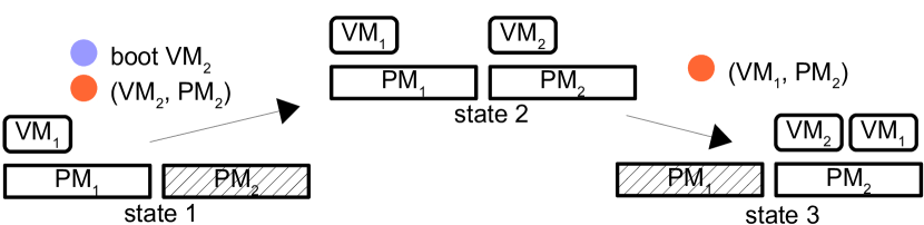
Figure 4: Example of state transitions based on control actions.

The time-based aspect of a schedule is illustrated in Fig. 5. Past events that occurred before the current moment $t_{c}$, such as a VM migration at $time=1$ or a new user request to boot a VM at $time=4$, determine the current cloud state. Based on the past values of different geotemporal variables, such as electricity prices $e_{i}$ and $e_{i+1}$ at different data center locations, we are able to get their value forecasts in the forecast window. Different control actions of a schedule inside the forecast window can then be tried out at any moment between $t_{c}$ and $t_{f}$. The control actions can be evaluated to determine the resulting VM locations and estimate costs with regard to the different geotemporal input forecasts and other optimisation problem aspects, such as constraints or SLA violations. When a schedule has been selected for execution, any immediate actions are applied and the forecast window moves as time passes, new requests arrive and geotemporal inputs change.

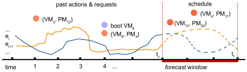
Figure 5: Schedule optimisation inside a forecast window.

5.4 Hybrid Genetic Algorithm Implementation

We now present the hybrid genetic algorithm. The most challenging parts in its design were the genetic operators that had to semantically match our optimisation problem domain, the fitness function that combines the decision support components and the hybrid part of the algorithm, i.e. the greedy local improvement. 

5.4.1 Schedule Fitness

In a genetic algorithm, we keep not only one, but a population of multiple problem solutions – multiple cloud control schedules, in our case. An essential part of the algorithm is to evaluate the fitness of each of these schedules. The fitness function we derived for this purpose is adapted from the decision support components, but constrained only to the forecast window (as we cannot affect actions that were already executed or plan further ahead than the available forecasts). Additional decision support components can be treated in a similar manner. 

For a schedule $s$, we calculate the capacity and allocation constraint fitness, as a measure of how well the VM s are allocated and the PM s are within their capacity, using the time-weighted function:

$$constraint(s)={\sum}_{\forall t\in fw}\frac{w_{alloc}\cdot R_{unalloc,t}+w_{cap}\cdot R_{overcap,t}}{|fw|}$$ (17)

where $R_{unalloc,t}$ and $R_{overcap,t}$ are ratios of $vm,\forall vm\in VMs_{t}$ for which $C_{1}$ (Eq. 15) does not hold and $pm,\forall pm\in PMs$ for which $C_{2}$ (Eq. 16) does not hold at moment $t$, respectively. $|fw|$ is the cardinality of $fw$ (the number of time periods in the interval). Constants $w_{alloc}$ and $w_{cap}$ in $[0,1]$ define the components’ weights.

The acceptable migration rate $R_{mig\_min}$ and the maximum allowed migration rate $R_{mig\_max}$ can be specified in the SLA, or determined by the cloud provider’s bandwidth expenses. Their values are used to calculate the QoS component from the actual migration rate $R_{mig}$ over the period of $fw$.

$$qos\_pen(vm)=\left\{\begin{array}[]{ll}0&\mbox{if }R_{mig}<R_{mig\_min}\\ 1&\mbox{if }R_{mig}>R_{mig\_max}\\ \frac{R_{mig}-R_{mig\_min}}{R_{mig\_max}-R_{mig\_min}}&\mbox{otherwise.}\end{array}\right.$$ (21)

The $qos\_pen$ expression gives a penalty for too frequent migrations per VM s that grows linearly from 0 to 1 for the migration rate $R_{mig}$ from $R_{mig\_min}$ to $R_{mig\_max}$. We then calculate the average QoS penalty over all the VM s.

$$qos(s)=\frac{{\sum}_{\forall vm\in VMs_{t_{c}}}qos\_pen(vm)}{|VMs_{t_{c}}|}$$ (22)

As a cost estimation, we use a simplified expression – $utilprice$. First, we calculate the average value of utilisation multiplied by $pPUE$ and $e$ over all PM s in the forecast window. This is a heuristic of the total energy costs from Eq. 14.

$$up\_avg(s)=\frac{{\sum}_{\forall pm\in PMs}{\sum}_{\forall t\in fw}util_{t}(pm)\cdot pPUE_{loc(pm),t}\cdot e_{loc(pm),t}}{|PMs|\cdot|fw|}$$ (23)

Then we normalise it to a $[0,1]$ interval by dividing it with $up\_worst$, which is the same as $up\_avg$, but calculated for a constant maximum utilisation $util_{t}(pm)=1$.

$$utilprice(s)=\frac{up\_avg(s)}{up\_worst}$$ (24)

To measure how tightly VM s are packed among the available PM s, we estimate the consolidation quality $consolid$ by considering only positive utilisation time series elements denoted as $\{pos\_util_{t}(pm):t\in fw,\ \text{ s.t. }util_{t}(pm)>0\}$.

$$consolid(s)=1-\frac{1}{|PMs|}{\sum}_{\forall pm\in PMs}\frac{{\sum}_{\forall t\in fw}pos\_util_{t}(pm)}{|pos\_util(pm)|}$$ (25)

Finally, we can calculate the fitness as:

$$\begin{split}fitness(s)=w_{ct}\cdot constraint(s)+w_{q}\cdot qos(s)+\\ +w_{up}\cdot utilprice(s)+w_{cd}\cdot consolid(s)\end{split}$$ (26)

with $w_{ct}$, $w_{q}$, $w_{up}$ and $w_{cd}$ in $[0,1]$ determining each component’s impact. The optimal schedule converges towards a fitness of 0 and the worst schedule towards 1. This solution evaluation form suits the forward compatibility requirement, as it can easily be extended with new decision support components by weighing them into the total fitness summation.

5.4.2 Genetic Operators

The creation procedure creates a random schedule as a time series of actions $(vm,pm),\ vm\in VMs_{t_{c}},pm\in PMs$ at random times $t_{r}\ \in fw$. The number of migrations is uniformly distributed between the parameters $min\_migrations$ and $max\_migrations$.

Given schedules $s_{1}$ and $s_{2}$, the crossover operator creates a child schedule $s_{3}$ by choosing a random moment $t_{r}\ \in[t_{c},t_{f}]$:

$$s_{3}=\left\{\begin{array}[]{ll}s_{1,t}:&t\in[t_{c},t_{r}],\\ s_{2,t}:&t\in[t_{r},t_{f}]\end{array}\right\}$$ (29)

The mutation operator applied to a schedule $s$ removes a random action $a$ and inserts one at a random moment $t_{r}\ \in fw$:

$$s=s\setminus a\cup\{t_{r}:(vm,pm)\},\\ a\in s,vm\in VMs_{t_{c}},pm\in PMs$$ (30)

TABLE II: Simulation parameters

period	duration	d	p (CPU; RAM)	v (CPU; RAM)	$P_{peak}$	$P_{peak}$	$(\mu_{P},\sigma_{P}^{2})$	$R_{mig\_min}$	$R_{mig\_max}$	$R$	$D$	$V_{thd}$
1 h	2 weeks	6	2,000 (8-16; 16-32)	10,000 (1-2; 2-4)	200	100	(0, 25)	1/4	1	1 Gb/s	0.3 Gb/s	0.1 Gb/s

TABLE III: Optimisation engine parameters

fw	pop	gen	cross	mut	rand	$min\_migr$	$max\_migr$	$w_{up}$	$w_{ct}$	$w_{alloc}$	$w_{cap}$	$w_{q}$	$w_{cd}$
12 h	100	100	0.15	0.05	0.3	0	$fw|VMs_{t_{c}}|/3$	0.4	0.1	0.4	0.6	0.4	0.1

5.4.3 Algorithm

The core genetic algorithm (GA) is listed in Alg. 1. Among other parameters not introduced so far, it also receives the population size $pop$, crossover, mutation and random creation rates $cross$, $mut$ and $rand$ in $[0,1]$ and the maximum number of generations $gen$.

Algorithm 1 Core genetic algorithm.

1:$schedules=create\_population(pop,rand,[existing])$

2:$i=0$

3:while $True$ do

4:     $calculate\_fitness(schedules)$ $\triangleright$ Eq. 26

5:     sort $schedules$ by fitness, best first

6:     if $i=gen$ then

7:         break loop

8:     end if

9:     $parents=roulette\_wheel(schedules,cross)$

10:     $children=crossover(parents)$ $\triangleright$ Eq. 29

11:     $schedules=schedules[0:pop\cdot(1-cross)]+children$

12:     $mutation(schedules,mut)$ $\triangleright$ Eq. 30

13:     $i=i+1$

14:end while

15:$existing=schedules$

16:return $schedules[0]$

After creating the population, every schedule is evaluated using the fitness function (Eq. 26) in line 4. Schedules are selected for crossover using the roulette wheel selection method with chances for selection proportional to a schedule’s fitness. A new generation is created by replacing the worst schedules with the newly created children (line 11). A random segment of the population proportional to $mut$ is changed by applying the mutation operator (line 12). The termination condition is fulfilled after $gen$ generations have passed (line 6) and the best schedule is returned. To cope with forecast-based planning, an existing population is partially propagated to the next schedule reevaluation, after the forecast window moves (line 1).

The GA is not guaranteed to satisfy all the constraints within a limited time period. To remedy this, we expand the optimisation with a greedy constraint satisfaction algorithm that is applied to the best schedule selected by the genetic algorithm to reallocate any offending VM s using a best cost fit (BCF) heuristic we developed that also considers geotemporal inputs.

The greedy constraint satisfaction pseudo-code is listed in Alg. 2. The algorithm receives as input $schedule$, the output of the GA. We begin by marking for reallocation all VM s which cause any hard constraint violations ($C_{1}$ or $C_{2}$) in line 2 and additionally all VM s from underutilised hosts in line 3. The VM s will then be reallocated in the outermost loop (line 5) starting with larger VM s first whose placement is more constrained (line 4). Available PM s are split into $active$ and $nonactive$ lists, depending on whether they are suspended or not. We sort $inactive$ in line 8 such that larger PM s come first for activation (preferable to more smaller machines, because of the idle power overhead) and data centers with lower combined electricity price and cooling overhead cost are preferred. The target PM to host $vm$ is selected in the inner loop in line 10 by first sorting $active$ to try and fill out almost full PM s first and prefer lower-cost location in case of ties (line 11) and activating the next PM from $inactive$ if $vm$ does not fit any of the $active$ PM s (line 19). When a fitting PM is found, the action is added to $schedule$ and the algorithm continues with the next VM.

Algorithm 2 Greedy constraint satisfaction – BCF heuristic.

1:$to\_alloc=$ empty list

2:append all constraint-violating VM s to $to\_alloc$

3:append VM s from all underutilised PM s to $to\_alloc$

4:sort $to\_alloc$ by resource requirements decreasing

5:for $vm\in to\_alloc$ do

6:     $active=$ all PMs where at least one VM is allocated

7:     $inactive=$ all PMs where no VMs are allocated

8:     sort $inactive$ by capacity decreasing, cost increasing 

9:     $mapped=False$

10:     while not $mapped$ do

11:         sort $active$ by free capacity, cost increasing

12:         for $pm\in active$ do

13:              if $vm$ fits $pm$ then

14:                  $mapped=True$

15:                  break loop

16:              end if

17:         end for

18:         if not $mapped$ then

19:              pop $inactive[0]$ and append it to $active$

20:         end if

21:     end while

22:     modify $schedule$ by adding a migration $(vm,pm)$

23:end for

24:return $schedule$

6 Evaluation

We evaluated the proposed progressive cloud controller in a large-scale simulation of 10k VM s based on real traces of geotemporal inputs. To be able to simulate cloud behaviour under geotemporal inputs, we developed our own open source simulator Philharmonic. The goals of the evaluation are: (1) Estimate energy and cost savings, as well as the QoS  attainable using the pervasive cloud controller; (2) Analyse the impact of various inputs, such as data center geography, different geotemporal inputs or controller parameters; (3) Validate the pervasive cloud controller extensibility by running the simulator with different decision support component subsets; (4) Define cloud provider guidelines, such as how temperature variation or forecast data quality affect the energy savings and illustrate their usage in a case study.

6.1 Evaluation Methodology

In this part we give an overview of the simulator’s implementation and proceed with explaining all the simulation details, such as the datasets, parameters and the baseline controller.

6.1.1 Philharmonic Simulator

A high-level overview of the Philharmonic simulator [39] that we developed is shown in Fig. 6. A simulation in Philharmonic consists of iterating through a series of equally-spaced time periods, collecting the currently available electricity price and temperature forecasts, as well as the incoming VM requests from the environment component. The controller is called with the data known at that moment about the environment and the cloud to reevaluate the schedule for the forecast window and potentially schedule new or different actions. The simulator applies any actions scheduled for the current moment on the cloud model and continues with the next time step, repeating the procedure. The applied actions are used to calculate the resulting energy consumption and electricity costs, using the model from Section 4.

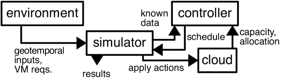
Figure 6: Philharmonic simulator overview.

6.1.2 Simulation Details

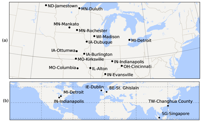
Figure 7: Cities used as data center locations in the simulation based on a: (a) US dataset (b) world-wide dataset.

Real historical traces for electricity prices and temperatures were used in the simulation for 15 cities in the USA shown in Fig. 7 (a). The electricity price dataset described in [17] was used. The temperatures were obtained from the Forecast web service [18]. To evaluate less correlated geotemporal inputs, we used a world-wide dataset for six cities accross three continents shown in Fig. 7 (b), choosing non-US cities to match the locations of Google’s data centers. Temperatures were again obtained from the Forecast API [18]. Due to lack of RTEP data for the four non-US cities, we artificially generated these traces from the data known for other US cities. We shifted the time series based on the time zone offsets and added a difference in annual mean values to resemble local electricity prices.

User requests for VM s were generated randomly by uniformly distributing the creation time and duration. The specifications of the requested VM s were modelled by normally distributing each resource type. An example VM request distribution is illustrated in Fig. 8. Available cloud infrastructure was generated by uniformly distributing physical machines among different data centers. Capacities for each each machine’s resources were generated in the same manner as the VM requests.

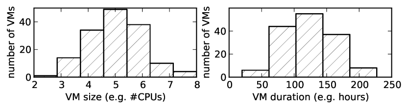
Figure 8: VM request resource and duration histogram.

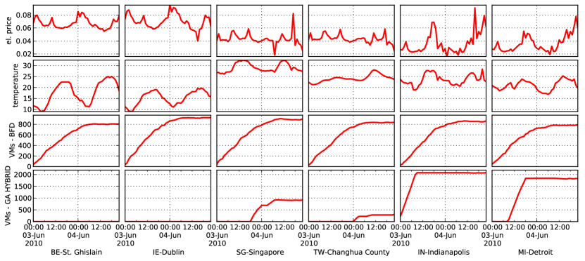
Figure 9: Dynamic VM management comparison of the controllers.

The exact simulation parameters used in the evaluation are listed in Table II. The time is defined by its period (simulation step size) and the total duration that determines the number of steps. To define the cloud, the number of data centers is given as $d$ (for the world-wide scenario, for the US scenario we consider $d=15$), and for $PMs$ and $VMs$ their number $p$ and $v$ (of boot requests in case of VM s – there were about 50% as much delete events as well) with minimum and maximum resource values in parentheses for the resources we assumed in this simulation – number of CPUs and the amount of RAM in GB. Besides running the simulation for the large-scale scenario with 10k VM s, we also simulated 100 and 1k VM s, but as the difference in normalised savings was only marginal, we only include the large-scale results. Uniform resource weights were used in the $util$ function (Eq. 10). We used $P_{peak}$ with $P_{idle}$ values $50\%$ of the peak, as reported in [40], and added normal random noise of the form $\mathcal{N}\ (\mu_{P},\sigma_{P}^{2})$ to account for load variation. $R_{mig}$ was calculated hourly and constant migration model parameters ($R$, $D$, $V_{thd}$) were used. We used these settings in all the simulations, unless otherwise specified.

As a baseline controller for results comparison, we implemented a method for VM consolidation dynamically adapting to user requests using a best fit decreasing (BFD) placement heuristic developed by Beloglazov et al. in [37]. We implemented the updated version of the controller that is currently developed for inclusion in the OpenStack open source cloud manager as project Neat [16]. Based on our classification of related work, this is a level two cloud management method that dynamically reallocates VM s, treating all energy uniformly.

The optimisation engine’s algorithm parameters are listed in Table III. All the weights used in the fitness function (Eq. 26) were systematically calibrated using automated parameter exploration, which we cover later. The values listed in the table show the parameter combination that achieved the highest energy savings with the least number of constraint violations.

6.2 Dynamic Controller Analysis

This part of the analysis aims to compare our pervasive cloud controller with the baseline controller by visualising individual actions. The use case is the scenario with world-wide data centers and other parameters we already described in Table II.

In Fig. 9 we see 6x4 graphs, where the columns represent data centers. First two rows show geotemporal inputs – electricity price and temperatures. The next two row shows the dynamic number of active VM s at the corresponding data center. The third row shows the behaviour of the baseline controller and the fourth row of the pervasive cloud controller. The x-axes of all the graphs cover the same time span and the graphs in the same column are aligned to the same x-axis, shown in the bottom. Similarly, the graphs in the same row share the same y-axis.

The electricity prices are lowest in the USA (with an increase towards the end of the day), followed by Asian locations and the European locations have significantly higher prices. Temperatures start the lowest in Europe, but then approach 20 C. The other locations oscillate around 20 C, except for the peaks in Asian locations where 30 C are approached. We can see that the baseline method roughly uniformly distributes the VM s across all the available data centers, disregarding the geotemporal inputs. The pervasive cloud controller allocates VM s in the first 18 hours filling out the US capacities, targeting lower electricity prices. No VM s are allocated in the European locations during this period, due to high electricity prices and enough capacity at other locations. The Asian locations are initially empty, but after the temperature peak is over, VM s are migrated to the Singapore data center and at the end of the first day (when Asian electricity prices start to decrease even bellow the US values), the Taiwan data center as well. This shows us the desired behaviour of the pervasive cloud controller where geotemporal inputs are monitored and adapted to by reallocating load to the most cost-efficient data center location.

6.3 Aggregated Simulation Results

To give an estimation of the benefits of using our pervasive cloud controller in a large-scale scenario described in Table II and analyse various environmental parameters, we collected the performed actions during the whole simulation and calculated the aggregated energy consumption and costs.

6.3.1 Cost Savings

The normalised results of the simulation based on the world-wide dataset with 10k VM s are shown in Fig. 10. A group of columns is shown for each of the examined quality metrics – IT energy, IT cost, total energy and total cost. Inside each group, there is a column for both of the scheduling algorithms: the baseline algorithm (BFD) and the pervasive cloud controller (GA HYBRID COST). The values are normalised as a relative value of the baseline algorithm’s results. The absolute values are listed in Table IV. The pervasive cloud controller achieves savings of $28.6\%$ in total energy cost compared to the baseline. We can see that significant savings can be achieved using our pervasive cloud controller, which is especially relevant for large cloud providers such as Google or Microsoft that spend over $40M annually on data center electricity costs [2].

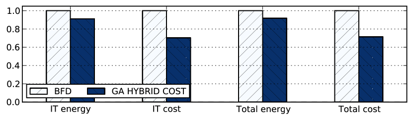
Figure 10: Normalised energy and costs of the pervasive cloud controller compared to the baseline method in a simulation of 10k VM s.

TABLE IV: Absolute energy consumption and costs

	BFD	GA HYBRID COST
IT energy (kWh)	6226.00	5673.63
IT cost ($)	309.40	217.64
Total energy (kWh)	7488.01	6869.55
Total cost ($)	370.20	264.39

6.3.2 Decision Support Component Variation

To validate the controller’s extensibility and show that it can work with different decision support components, we performed the same 10k VM simulation with different subsets of the decision support components considered by the optimisation engine. This analysis also gives an overview of the impact individual geotemporal inputs have in the total achieved energy savings.

The results are shown in Fig. 11. Each column stands for one of the simulation scenarios – both temperatures and electricity price components (GA ALL), electricity price component, but no temperature (GA NT) and no electricity price or temperature components (GA NE). Total cost savings of 7.5% are achieved when both components are considered compared to not considering temperatures. Savings are 13% when compared to not considering both components, which is a significant difference. In the same manner we turn on or off certain decision support components as a configuration option in the controller’s implementation, new geotemporal inputs and rules can be added in the future when necessary.

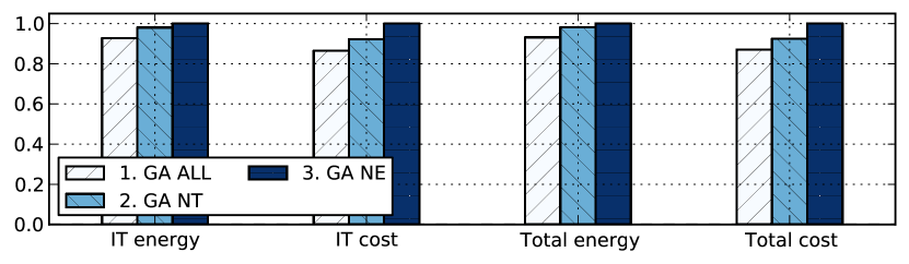
Figure 11: Normalised energy and costs of the pervasive cloud controller with various decision support components: temperature and electricity price (1), no temperature (2) and no temperature or electricity cost (3).

6.3.3 Geography Variation

Different cloud providers will have different data center locations and geographical distributions. To estimate the impact of this geographical distribution of data centers on the possible cost savings achievable using our scheduling method, we simulate its effects on two such scenarios – the world-wide scenario and the USA scenario, as described in Section 6.1. Furthermore, as the USA dataset of geotemporal inputs consists of real historical electricity price traces (which we did not have to artificially adapt to different time zones and local averages) it further testifies to the validity of our approach. Lastly, even though current cloud providers have incentives to spread their data centers further apart to bring services closer to a world-wide user base, with the advent of smart buildings [3] we might see more localised data center distributions based on neighborhood, city or region organisations.

The results of the simulation for the USA and world-wide dataset for 10k VM s are shown in Fig. 12. The simulation settings were the same we explained in Section 6.1, except for the locations of the physical machines. The baseline controller was run for the USA dataset (BFD USA), and we can see the normalised results compared to this baseline for the pervasive cloud controller simulated on the USA dataset (GA USA) and the world-wide dataset (GA WORLD). It can be seen that significant cost savings of 24% are achieved even for the USA-only scenario. The pervasive cloud controller’s energy consumption and costs are lower in the world-wide scenario than for the US-only data centers, though – a further 10% decrease is possible.

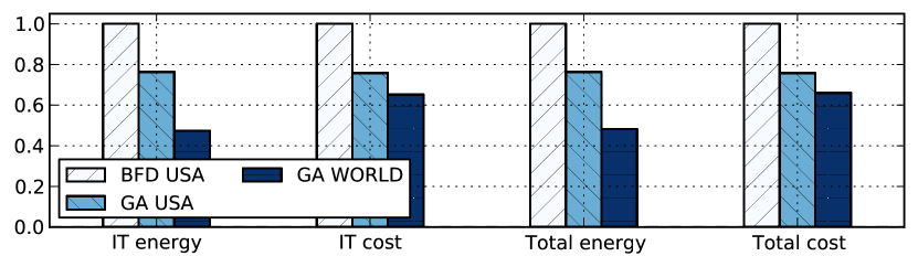
Figure 12: Normalised energy and costs of the pervasive cloud controller compared to the baseline method for the USA and world-wide datasets.

6.3.4 QoS Analysis

Aside from understanding the cost savings from the cloud provider’s perspective, we also have to analyse the QoS, i.e. how the controller affects end users of VM s. To measure this, we count how often the migration actions occur, i.e. the migration rate. To get more data, we ran the simulation to cover three months. A histogram of hourly migration rates of all the VM s obtained from the simulation of the pervasive cloud controller can be seen in Fig. 13. The two plots show different zoom levels, as there are progressively less hours with higher migration rates. Most of the time, no migrations are scheduled, with one migration per hour happening about $20\%$ of the time.

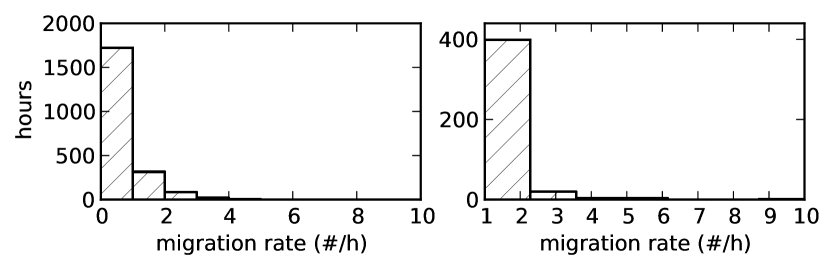
Figure 13: Hourly migration rate histogram (two zoom levels).

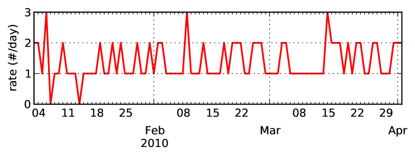
Figure 14: Aggregated worst-case per-VM migration rate.

To get a QoS metric meaningful to the user, we group migrations per VM  (as users are only interested in migrations of their own VM s) and process them in a function that aggregates migrations over a daily interval. We then define the aggregated worst-case metric by counting the migrations per VM per day and selecting the highest migration count among all the VM s in every interval. Such a metric could be useful e.g. in defining the lower bound for the availability rate in an SLA. The aggregated worst-case migration rate for the simulation of the pervasive cloud controller is shown in Fig. 14. There are one or two migrations per VM per day most of the time, with an occasional case with a higher rate such as the peaks with three migrations.

Given that this data is highly dependent of the scheduling algorithm parameters used and the actual environmental parameters for a specific cloud deployment, fitting one specific statistical distribution to the data to get the desired percentile value that can be guaranteed in an SLA would be hard to generalise for different use cases and might require manual modelling. Instead, we propose applying the distribution-independent bootstrap confidence interval method [41] to estimate the aggregated migration rate. In our simulation, the 95% confidence interval for the mean daily per-VM migration rate is 1.26–1.5 migrations per day.

6.3.5 Genetic Algorithm Parameter Exploration

To explore how the optimisation engine behaves under different GA  parameters, we ran the simulation with different parameter values and compared the resulting energy costs. We explored the weights of the different fitness function components in (Eq. 26). We developed a method for automatically running the simulation with different parameter combinations in the Philharmonic simulator. We covered a set $\{0,0.1,0.2,\ldots\ 1.\}$ for each of the four weight parameters, exploring all the combinations with a constraint that their sum equals 1 (as only weight ratios make a difference in the GA, not their absolute values), resulting in 285 combinations. This method can be used to calibrate the controller for different environments by finding the parameter combination that achieves the highest energy savings or the best QoS, similar to how different objectives are optimised in a Pareto frontier.

A radio chart with the results is shown in Fig. 15. The five axes show the four fitness component weights with the fifth axis as the energy cost expressed relative to the worst-case combination. One combination is shown as a pentagon of the same colour, indicating the 5-tuple $(w_{ct},w_{q},w_{cd},w_{up},cost)$. Combination colour is sorted by relative cost as well, with darker colours having higher and lighter colours lower energy costs. For clarity, we only show a subset of the combinations with the rounded relative cost closest to a step of 0.1. We can see that the lowest energy costs are achieved for high $w_{up}$ and $w_{q}$ weights, meaning that energy cost and a low number of migrations is prioritized. Higher energy costs were obtained when constraint satisfaction ($w_{ct}$) and VM consolidation ($w_{cd}$) is prioritized, as neither of these components includes geotemporal inputs.

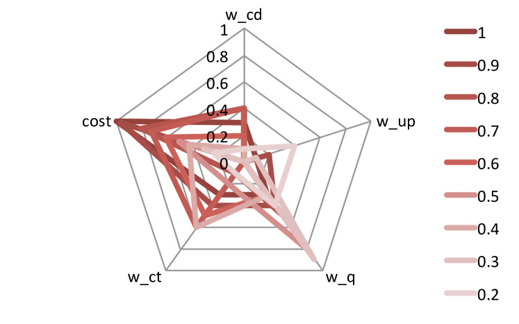
Figure 15: Relative energy costs for different GA parameters.

6.3.6 Temperature Range Variation

As different cloud providers have data centers at various locations, where temperature ranges can be very different, we analyse the impact of temperature range variation on pervasive cloud control effectiveness. Temperature variation is affected by the time of the year and the range of daily temperatures will vary over time. For this reason, we performed the simulation with different starting times throughout the year, which resulted in different temperature ranges for different simulation runs.

The resulting graphs are shown in Fig. 16. The figure to the left shows the energy cost (normalised as relative to the maximum vaule) resulting from the simulation of the pervasive cloud controller handling the same VM requests, only shifted to a different month of the year. We can see a gradual trend, with a single sudden drop in October. To extract the statistical environment changes between these runs, we plotted the same normalised cost as a scatter plot against the temperature variation in the figure to the right. The temperature variation is calculated as the mean of the standard deviations of temperature values for individual data center locations. Once ordered this way, the trend of the data becomes clearer and we calculated a linear correlation between the variables with an adjusted $R^{2}$ of 0.31 (model shown in red). We see that a higher temperature variation results in lower energy costs. This is due to the higher impact avoiding locations with unfavourable cooling efficiency conditions has.

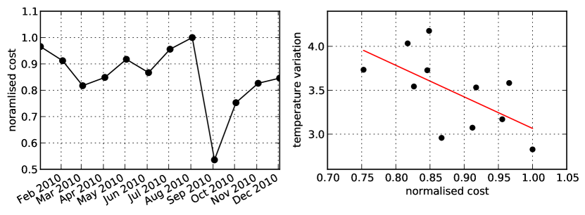
Figure 16: Energy costs for simulation runs during different months of the year (left) and a scatter plot of the same data and the temperature variation metric showing linear dependence (right).

6.3.7 Data Quality

To explore the effect errors in forecasting geotemporal inputs have on the pervasive cloud controller’s operation, we simulate different data quality scenarios. Additionally, we explore different forecast window sizes and their effect on scheduling efficiency. A longer forecast window enables the fitness function to evaluate the consequences of different management actions over a longer interval, reducing the impact of short-term geotemporal impact changes, such as electricity price spikes.

The time series provided to the scheduling algorithm with different forecasting errors were obtained using Eq. 6 by selecting different standard deviation ($\sigma_{pred}$) parameters. A $\sigma_{pred}$ close to zero represents very accurate forecasting, while a higher $\sigma_{pred}$ causes higher signal volatility and forecasting errors. A segment of the generated time series for one of the cities is shown in Fig. 17. Both time series are aligned to the same x-axis. Each curve represents one $\sigma_{pred}$ scenario. It can be seen that smaller error levels ($\sigma_{pred}$ of 3 $/MWh and 0.5 C for electricity or temperature, respectively) still retain the general trend with identifiable peaks and lows. Higher error levels ($\sigma_{pred}$ from 30 to 50 $/MWh or 3 to 5 C for electricity or temperature, respectively) start to significantly diverge from the original time series, in that peaks are predicted where in reality lows occur and vice versa. We simulated forecast window sizes of 4, 12, 24 and 48 hours.

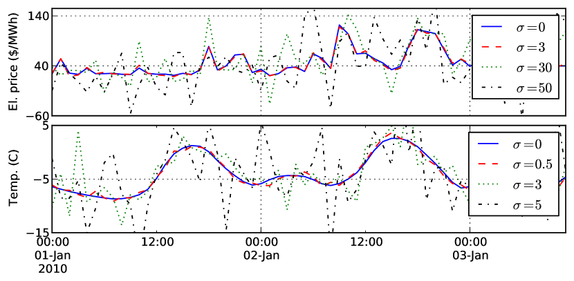
Figure 17: Different levels of forecasting errors applied to electricity price and temperature time series (for Mankato, MN).

The generated time series with forecasting errors were provided to the pervasive cloud controller to base its decisions upon. The forecast parameter exploration results are shown in Fig. 18. The 3-dimensional visualisation shows the space of forecast window sizes and electricity price $\sigma_{pred}$ values on the bottom plane. The z-position on the surface (its height) shows the total energy cost (including the migration and cooling overhead), normalised relative to the worst case ($fw=4\ h,\ \sigma_{pred}=50\ \$/MWh$). Missing data points were interpolated. The graph only shows $\sigma_{pred}$ used to model electricity price forecasting errors, but a matching $\sigma_{pred}$ for temperature from Fig. 17 was also applied.

Looking at the forecast window sizes in Fig. 18, we can see that initially bigger windows result in lower costs. This trend can clearly be seen from 4 h to 20 h for all $\sigma_{pred}$. The trend changes, however, for 24 h and bigger windows. Higher or lower savings are visible and the pattern is more randomised. The reason is that both electricity prices and temperatures exhibit a daily seasonality effect and extending the window further than 24 h does not provide much more information to the controller, but increases the problem search space. We conclude that the rift-like surface shape in the forecast window range from 12 to 24 hours represents an optimal size for the given geotemporal inputs.

The forecasting error dimension shows deviations of around 25% between large forecasting errors and perfect knowledge. This can be attributed to the fact that large forecasting errors mislead the controller into placing VM s in areas where geotemporal inputs are in fact worse, so both energy cost losses and migration overheads are incurred. Smaller forecasting errors result in lower energy costs, which shows the importance of having accurate forecasting methods (or data sources) when managing clouds based on geotemporal inputs. Based on our simulation, $\sigma_{pred}$ of 3 $/MWh (mean squared error (MSE) of $\approx 9$) and 0.5 C (MSE of $\approx 0.25$) or less is necessary for feasible cost savings.

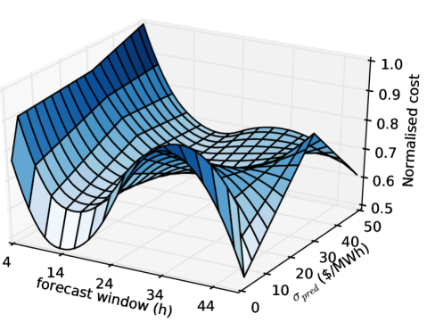
Figure 18: Normalised energy costs resulting from different forecasting errors and forecast window sizes.

6.4 Cloud Provider Guidelines Case Study

To show the usage potential of the collected measurements as guidelines, we performed a case study for several different cloud providers. The results are shown in Table V. The annual electricity cost estimations are obtained from [2]. We selected cloud providers of different scale (e.g. A and C). We compare several environment conditions, namely the temperature variation $temp\_var$ and data quality metrics $fw$ and $\sigma_{pred}$, considering different combinations as hypothetical scenarios that cloud providers might be in. The cost factor is calculated based on the already analysed temperature variation linear model from Fig. 16 and the forecast data quality impact results from Fig. 18. Finally, we show the order of magnitude of the cost savings based on the cost factor.

TABLE V: Cloud provider guidelines case study.

provider	electricity	$fw$	$\sigma_{pred}$	$temp\_var$	factor	savings
A	$38M	14	10	3.5	0.565	$16.5M
B	$36M	48	30	2.5	0.989	$0.4M
C	$12M	24	10	4.0	0.536	$5.6M

The results show that significant savings are possible using pervasive cloud control with appropriate environmental conditions. The B scenario, however, shows that even with high initial costs, having bad forecast data quality and a low temperature variation can result in lower savings, perhaps not enough of an incentive to apply our method. On the other hand, even a smaller provider, such as C, can achieve promising savings in a favourable environment.

7 Conclusion

In this paper we presented an approach for pervasive cloud control under geotemporal inputs, such as real-time electricity pricing and temperature-dependent cooling efficiency. The solution is designed for extensibility with new geotemporal inputs and cloud regulation mechanisms through a modular decision support component system and a forward-compatible optimisation engine. We presented a proof-of-concept controller implementation combining forecast-based planning and a hybrid genetic algorithm with greedy local optimisation. The genetic algorithm approach was extended with partial population propagation. 

The approach was evaluated in a simulation based on real traces of temperatures and electricity prices. We estimated energy cost savings of up to $28.6\%$ compared to a baseline cloud control method that applies VM consolidation without considering geotemporal inputs. We analysed per-VM migrations to show that no significant QoS impact is incurred in the process. We evaluated different parameters such as geographical data center distributions and forecast data quality as cloud provider guidelines to find conditions fit for pervasive cloud control. 

The questions that remain open are how to extend the method for integrated forecasting of arbitrary time series data, e.g. application-level load predictions or local renewable energy availability. Additionally, it would be beneficial to research the method in the context of containers and stateless applications which enable much more efficient computation migration. We plan to research these topics in our future work.

Dražen Lučanin is a PhD student at the Vienna University of Technology, studying energy efficiency in cloud computing. Previously, he worked as an external associate at the Ruđer Bošković Institute on machine learning methods for forecasting financial crises. He graduated with a master’s degree in computer science at the Faculty of electrical engineering and computing, University of Zagreb. For more information, please visit http://www.infosys.tuwien.ac.at/staff/drazen/

Ivona Brandic is Assistant Professor at the Vienna University of Technology. Prior to that, she was Assistant Professor at the Department of Scientific Computing, University of Vienna. She received her PhD degree in 2007 and her venia docendi for practical computer science in 2013, both from Vienna University of Technology. In 2011 she received the Distinguished Young Scientist Award from the Vienna University of Technology for her project on the Holistic Energy Efficient Hybrid Clouds. She published more than 50 scientific journal, magazine and conference publications and she co-authored a text-book on federated and self-manageable Cloud infrastructures. For more information, please visit http://www.infosys.tuwien.ac.at/staff/ivona/

References

- [1] Jonathan Koomey, “Growth in Data center electricity use 2005 to 2010,” Analytics Press, Oakland, CA, Tech. Rep., Aug. 2011. [Online]. Available: http://www.analyticspress.com/datacenters.html
- [2] A. Qureshi, R. Weber, H. Balakrishnan, J. Guttag, and B. Maggs, “Cutting the electric bill for internet-scale systems,” SIGCOMM Comput. Commun. Rev., vol. 39, no. 4, pp. 123–134, Aug. 2009.
- [3] G. Privat, “Smart Building Functional Architecture, FI.ICT-2011-285135 FINSENY D4.3,” Tech. Rep., 2013. [Online]. Available: http://www.fi-ppp-finseny.eu/wp-content/uploads/2013/04/FINSENY_D4.3_v1.01.pdf
- [4] X. Yang, Z. Zhou, S. Wallace, Z. Lan, W. Tang, S. Coghlan, and M. E. Papka, “Integrating Dynamic Pricing of Electricity into Energy Aware Scheduling for HPC Systems,” in Proceedings of the International Conference on High Performance Computing, Networking, Storage and Analysis, ser. SC ’13. New York, NY, USA: ACM, 2013, pp. 60:1–60:11.
- [5] R. Weron, Modeling and Forecasting Electricity Loads and Prices: A Statistical Approach, 1st ed. Wiley, Dec. 2006.
- [6] L. A. Barroso and U. Hölzle, “The datacenter as a computer: An introduction to the design of warehouse-scale machines,” Synthesis lectures on computer architecture, vol. 4, no. 1, pp. 1–108, 2009.
- [7] I. Goiri, W. Katsak, K. Le, T. D. Nguyen, and R. Bianchini, “Parasol and greenswitch: Managing datacenters powered by renewable energy,” in ACM SIGARCH Computer Architecture News, vol. 41. ACM, 2013, pp. 51–64.
- [8] K. Le, R. Bianchini, J. Zhang, Y. Jaluria, J. Meng, and T. D. Nguyen, “Reducing Electricity Cost Through Virtual Machine Placement in High Performance Computing Clouds,” in Proceedings of 2011 International Conference for High Performance Computing, Networking, Storage and Analysis, ser. SC ’11. New York, NY, USA: ACM, 2011, pp. 22:1–22:12.
- [9] Z. Liu, A. Wierman, Y. Chen, B. Razon, and N. Chen, “Data center demand response: Avoiding the coincident peak via workload shifting and local generation,” Performance Evaluation, vol. 70, no. 10, pp. 770–791, Oct. 2013.
- [10] A. Berl, G. Lovász, F. von Tüllenburg, and H. de Meer, “Modelling Power Adaption Flexibility of Data Centres for Demand-Response Management,” in Energy Efficiency in Large Scale Distributed Systems. Springer, 2013, pp. 63–66.
- [11] H. Xu, C. Feng, and B. Li, “Temperature aware workload management in geo-distributed datacenters,” in Proceedings of the ACM SIGMETRICS/international conference on Measurement and modeling of computer systems, vol. 41. ACM, 2013, pp. 373–374.
- [12] E. Feller, L. Rilling, and C. Morin, “Snooze: A Scalable and Autonomic Virtual Machine Management Framework for Private Clouds,” in Proceedings of the 2012 12th IEEE/ACM International Symposium on Cluster, Cloud and Grid Computing (Ccgrid 2012), ser. CCGRID ’12. Washington, DC, USA: IEEE Computer Society, 2012, pp. 482–489.
- [13] A. Beloglazov and R. Buyya, “Managing Overloaded Hosts for Dynamic Consolidation of Virtual Machines in Cloud Data Centers Under Quality of Service Constraints,” IEEE Transactions on Parallel and Distributed Systems, vol. 24, no. 7, pp. 1366–1379, 2013.
- [14] M. Maurer, I. Brandic, and R. Sakellariou, “Enacting SLAs in clouds using rules,” Euro-Par 2011 Parallel Processing, pp. 455–466, 2011.
- [15] H. Liu, C.-Z. Xu, H. Jin, J. Gong, and X. Liao, “Performance and energy modeling for live migration of virtual machines,” in Proceedings of the 20th international symposium on High performance distributed computing, 2011, pp. 171–182.
- [16] A. Beloglazov and R. Buyya, “OpenStack Neat: A Framework for Dynamic and Energy-Efficient Consolidation of Virtual Machines in OpenStack Clouds,” Concurrency and Computation: Practice and Experience (CCPE), 2014.
- [17] S. Alfeld, C. Barford, and P. Barford, “Toward an analytic framework for the electrical power grid,” in Proceedings of the 3rd International Conference on Future Energy Systems: Where Energy, Computing and Communication Meet, ser. e-Energy ’12. New York, NY, USA: ACM, 2012, pp. 9:1–9:4.
- [18] “Forecast,” 2015. [Online]. Available: http://forecast.io/
- [19] L. Rao, X. Liu, L. Xie, and W. Liu, “Minimizing Electricity Cost: Optimization of Distributed Internet Data Centers in a Multi-Electricity-Market Environment,” in 2010 Proceedings IEEE INFOCOM, Mar. 2010, pp. 1–9.
- [20] M. Lin, Z. Liu, A. Wierman, and L. Andrew, “Online algorithms for geographical load balancing,” in Green Computing Conference (IGCC), 2012 International, Jun. 2012, pp. 1–10.
- [21] J. Li, Z. Li, K. Ren, and X. Liu, “Towards Optimal Electric Demand Management for Internet Data Centers,” IEEE Transactions on Smart Grid, vol. 3, no. 1, pp. 183–192, Mar. 2012.
- [22] J. Doyle, R. Shorten, and D. O’Mahony, “Stratus: Load Balancing the Cloud for Carbon Emissions Control,” IEEE Transactions on Cloud Computing, vol. 1, no. 1, pp. 1–1, Jan. 2013.
- [23] N. Buchbinder, N. Jain, and I. Menache, “Online Job-Migration for Reducing the Electricity Bill in the Cloud,” in NETWORKING 2011, ser. Lecture Notes in Computer Science, J. Domingo-Pascual, P. Manzoni, S. Palazzo, A. Pont, and C. Scoglio, Eds. Springer Berlin Heidelberg, Jan. 2011, no. 6640, pp. 172–185.
- [24] H. Guler, B. Cambazoglu, and O. Ozkasap, “Cutting Down the Energy Cost of Geographically Distributed Cloud Data Centers,” in Energy Efficiency in Large Scale Distributed Systems. Vienna: Springer Berlin Heidelberg, 2013, pp. 279–286.
- [25] Z. Liu, Y. Chen, C. Bash, A. Wierman, D. Gmach, Z. Wang, M. Marwah, and C. Hyser, “Renewable and cooling aware workload management for sustainable data centers,” in Proceedings of the 12th ACM SIGMETRICS/PERFORMANCE joint international conference on Measurement and Modeling of Computer Systems, ser. SIGMETRICS ’12. New York, NY, USA: ACM, 2012, pp. 175–186.
- [26] S. Ren, Y. He, and F. Xu, “Provably-Efficient Job Scheduling for Energy and Fairness in Geographically Distributed Data Centers,” in 2012 IEEE 32nd International Conference on Distributed Computing Systems (ICDCS), Jun. 2012, pp. 22 –31.
- [27] M. Kesavan, I. Ahmad, O. Krieger, R. Soundararajan, A. Gavrilovska, and K. Schwan, “Practical Compute Capacity Management for Virtualized Datacenters,” IEEE Transactions on Cloud Computing, vol. 1, no. 1, pp. 1–1, Jan. 2013.
- [28] C. Mastroianni, M. Meo, and G. Papuzzo, “Probabilistic Consolidation of Virtual Machines in Self-Organizing Cloud Data Centers,” IEEE Transactions on Cloud Computing, vol. 1, no. 2, pp. 215–228, Jul. 2013.
- [29] M. D. Cauwer and B. O’Sullivan, “A Study of Electricity Price Features on Distributed Internet Data Centers,” in Economics of Grids, Clouds, Systems, and Services - 10th International Conference, GECON 2013, Zaragoza, Spain, September 18-20, 2013. Proceedings, ser. Lecture Notes in Computer Science, J. Altmann, K. Vanmechelen, and O. F. Rana, Eds., vol. 8193. Springer, 2013, pp. 60–73.
- [30] Z. Abbasi, T. Mukherjee, G. Varsamopoulos, and S. K. S. Gupta, “Dynamic hosting management of web based applications over clouds,” in 2011 18th International Conference on High Performance Computing (HiPC), Dec. 2011, pp. 1–10.
- [31] X. Zhu, L. Yang, H. Chen, J. Wang, S. Yin, and X. Liu, “Real-Time Tasks Oriented Energy-Aware Scheduling in Virtualized Clouds,” IEEE Transactions on Cloud Computing, vol. 2, no. 2, pp. 168–180, Apr. 2014.
- [32] X.-B. Hu, W.-H. Chen, and E. Di Paolo, “Multiairport Capacity Management: Genetic Algorithm With Receding Horizon,” IEEE Transactions on Intelligent Transportation Systems, vol. 8, no. 2, pp. 254–263, Jun. 2007.
- [33] J. Kolodziej, S. U. Khan, L. Wang, A. Byrski, N. Min-Allah, and S. A. Madani, “Hierarchical genetic-based grid scheduling with energy optimization,” Cluster Computing, vol. 16, no. 3, pp. 591–609, 2013.
- [34] F. Larumbe and B. Sanso, “A Tabu Search Algorithm for the Location of Data Centers and Software Components in Green Cloud Computing Networks,” IEEE Transactions on Cloud Computing, vol. 1, no. 1, pp. 22–35, Jan. 2013.
- [35] D. Meisner, B. T. Gold, and T. F. Wenisch, “PowerNap: eliminating server idle power,” SIGPLAN Not., vol. 44, no. 3, pp. 205–216, Mar. 2009.
- [36] D. E. Goldberg, Genetic algorithms in search, optimization, and machine learning. Addison-wesley Reading Menlo Park, 1989, vol. 412.
- [37] A. Beloglazov, J. Abawajy, and R. Buyya, “Energy-aware resource allocation heuristics for efficient management of data centers for Cloud computing,” Future Generation Computer Systems, vol. 28, no. 5, pp. 755–768, May 2012.
- [38] G. Mélard and J.-M. Pasteels, “Automatic ARIMA modeling including interventions, using time series expert software,” International Journal of Forecasting, vol. 16, no. 4, pp. 497–508, Oct. 2000.
- [39] Dražen Lučanin, “Philharmonic,” 2014. [Online]. Available: https://philharmonic.github.io/
- [40] X. Fan, W.-D. Weber, and L. A. Barroso, “Power provisioning for a warehouse-sized computer,” in Proceedings of the 34th annual international symposium on Computer architecture, ser. ISCA ’07. New York, NY, USA: ACM, 2007, pp. 13–23.
- [41] B. Efron and R. J. Tibshirani, An Introduction to the Bootstrap. CRC Press, May 1994.