Hard X-ray view on intermediate polars in the Gaia era

Abstract

The hardness of the X-ray spectra of intermediate polars (IPs) is determined mainly by the white dwarf (WD) compactness (mass-radius ratio, $M/R$) and, thus, hard X-ray spectra can be used to constrain the WD mass. An accurate mass estimate requires the finite size of the WD magnetosphere $R_{\rm m}$ to be taken into the account. We suggested to derive it either directly from the observed break frequency in power spectrum of X-ray or optical lightcurves of a polar, or assuming the corotation. Here we apply this method to all IPs observed by NuSTAR (10 objects) and Swift/BAT (35 objects). For the dwarf nova GK Per we also observe a change of the break frequency with flux, which allows to constrain the dependence of the magnetosphere radius on the mass-accretion rate. For our analysis we calculated an additional grid of two-parameter ($M$ and $R_{\rm m}/R$) model spectra assuming a fixed, tall height of the accretion column $H_{\rm sh}/R=0.25$, which is appropriate to determine WD masses in low mass-accretion IPs like EX Hya. Using the Gaia Data Release 2 we obtain for the first time reliable estimates of the mass-accretion rate and the magnetic field strength at the WD surface for a large fraction of objects in our sample. We find that most IPs accrete at rate of $\sim 10^{-9}$ M_⊙ yr^-1, and have magnetic fields in the range 1–10 MG. The resulting WD mass average of our sample is $0.79\pm 0.16$ M_⊙, which is consistent with earlier estimates.

1 Introduction

Intermediate polars (IPs) are a subclass of cataclysmic variables (CVs), accreting close binary systems with white dwarfs (WDs) as accretors and main sequence dwarfs, overfilling their Roche lobe, as donors (see details in Warner, 2003). The WDs in IPs are magnetized enough (0.1–10 MG) to destroy the accretion disc at some distance (the magnetospheric radius $R_{\rm m}$), but not enough to push the magnetosphere beyond the corotation radius $R_{\rm c}$ and inhibit the accretion. Here $R_{\rm c}$ is defined as the radius where the Kepler frequency in the accretion disc equals the spin frequency of the WD. At smaller radii, accreting material falls along magnetic field lines onto the WD surface forming a standing shock above the surface, where the kinetic energy of the falling matter is transformed into thermal energy, and radiated away as optically thin plasma emission with typical temperatures of a few tens keV (Aizu, 1973; Fabian et al., 1976). The plasma thus cools by radiation and settles in a subsonic regime below the shock. This region is usually referred to as a post-shock region (PSR) or an accretion column.

Hard X-ray radiation of a PSR allows to evaluate the WD mass $M$, because the post-shock temperature is determined mainly by the compactness of the WD (Katz, 1977; Rothschild et al., 1981). This idea was further developed and exploited to estimate masses of several WDs (Wu et al., 1994; Cropper et al., 1998; Cropper et al., 1999; Ramsay, 2000). These authors developed the PSR theory to very high sophistication including cyclotron cooling, the dipole geometry of PSRs, and the possible difference between electron and proton temperatures (Canalle et al., 2005; Saxton et al., 2007). In these works, however, X-ray spectra in the classical X-ray band ($<20$ keV) were considered. This resulted in large uncertainties for the determined masses as the Wien exponential cutoff of the PSR spectra, which is essential for an accurate determination of the temperature, occurs at higher energies.

More reliable results on WD masses in IPs were obtained after the launch of X-ray observatories designed for the hard X-ray band. Mass determinations using the PSR model spectra were performed using data from RXTE/HEXTE (Suleimanov et al., 2005), Swift/BAT (Brunschweiger et al., 2009), and Suzaku (Yuasa et al., 2010; Hayashi & Ishida, 2014b; Yuasa et al., 2016) observatories. Several IPs were investigated also using INTEGRAL/IBIS observations (Revnivtsev et al., 2004; Falanga et al., 2005), however, most of them were interpreted assuming generic hot optically thin plasma radiation models rather than PSR models calculated from first principles (Barlow et al., 2006; Landi et al., 2009; Bernardini et al., 2012). Given the importance of the cutoff for WD mass measurements, and comparatively faintness of IPs in the hard band, currently the data provided by the NuSTAR observatory (Harrison et al., 2013) suit best for this purpose. Several IPs were studied by NuSTAR using PSR model spectra (Hailey et al., 2016; Suleimanov et al., 2016; Shaw et al., 2018; Wada et al., 2018). A recent review of hard X-ray emitting IPs was presented by Mukai (2017).

The commonly used method for mass determination of WDs in IPs described above is not without flaws. There are several theoretical uncertainties which can affect the results, most notably the assumed geometry of the PSR and the finite but not well defined magnetospheric radius. For the PSR geometry the dipole approximation appears to be well justified, and an accurate theory to calculate its structure has been developed by Canalle et al. (2005). A simplified approach has been suggested by Hayashi & Ishida (2014a), where the dipole geometry is approximated by a PSR cross-section increasing with distance from the WD surface.

Using of this simplified approach allowed Suleimanov et al. (2016) to take also the finite magnetosphere size into account. The latter development is particularly important for objects with relatively small magnetospheres with radii of a few WD radii $R$. Matter starting to fall from a small radius accelerates to significantly smaller velocities compared to the case of accretion from infinity. As a result, the WD mass might be significantly underestimated if this effect is not accounted for (Suleimanov et al., 2005). Whether the assumed magnetospheric radius affects the resulting WD mass estimate is not known a priori, because that PSR modeling of the X-ray spectra only allows to constrain $M-R_{\rm m}/R$.

Suleimanov et al. (2016) computed a two-parameter ($M$ and $R_{\rm m}/R$) grid of PSR model spectra in order to obtain such constraints from observations. To break the degeneracy and estimate the mass of the WD, an independent estimate of the magnetosphere size is required. Suleimanov et al. (2016) suggested to use the break frequency in the power spectrum of the studied IP assuming that it corresponds to the Keplerian frequency of the disc at the magnetospheric radius (Revnivtsev et al., 2009b, 2011). The method was applied to two IPs with small magnetospheres, EX Hya and GK Per, and indeed it was found that under this assumption the resulting mass estimates better agree with other estimates. For GK Per, which was observed in different luminosity states, we were also able to investigate the dependence of the magnetospheric radius on the mass-accretion rate (Suleimanov et al., 2016).

Another theoretical uncertainty is related to the generally unknown local mass-accretion rate $a$ (g s^-1 cm^-2). Indeed, PSRs with low $a$ and, therefore, low plasma density are expected to cool slowly and thus a larger shock height can be expected. This reduces the free-fall velocity at the shock, i.e., it might also lead to an underestimation of the WD mass. Luna et al. (2018) mentioned the significance of the PSR height for the low-luminosity IP EX Hya. In this paper we present a new two-parameter grid of PSR model spectra where this effect is quantified, and apply it to several IPs accreting at low rate.

The spectra of some luminous IPs, such as V1223 Sgr, have a very complicated structure at low photon energies ($<10$ keV), presumably due to complex absorption within the binary system or/and reflection off the WD’s surface (see, e.g. Cropper et al., 1998; Cropper et al., 1999; Suleimanov et al., 2005). Commonly, a partially covering absorber is considered to model the observed spectra (see, e.g., Cropper et al., 1999). Indeed, IPs rotate and the radiating PSR is expected to be periodically occulted by material falling along magnetic force lines (accretion curtains). As a typical observation duration is much longer than the IP spin period, part of the time only strongly absorbed emission from the PSR is observed. This effect is expected to be more pronounced for systems accreting at high rate where the density of the accretion flow is higher, which does indeed seem to be the case.

An additional aspect to explain the observed spectra is to include the reflection component (Cropper et al., 1998). This scenario is also physically motivated because the PSR radiation has to be reflected from the WD surface. Moreover, the iron-line complex at 6–7 keV observed in the majority of IPs is more readily explained in this scenario. We note, however, that the transmission of hard X-ray radiation through cold matter will also generate an iron fluorescence line. Moreover, the contribution of $K_{\alpha}$ is small in the spectra of low-luminosity IPs (e.g., EX Hya Luna et al., 2015) and large (more than a half of the total equivalent width of the complex) in the high-luminosity IPs like GK Per during outburst (Yuasa et al., 2016).

On the other hand, the importance of reflection was recently established for some IPs using NuSTAR observations (Mukai et al., 2015), and proved to be an important factor to be taken into account when determining the WD mass using broadband spectra (Shaw et al., 2018). We note, however, that detailed calculations of the reflected spectrum taking the geometry of the PSR into the account are required for such estimates to be robust, and no such calculations are available as of now. Furthermore, the relative importance of partially covering absorption and reflection components is still unknown and ignoring either effect could bias the mass estimates. In the present work we restrict, therefore, the analysis to hard X-rays ($>20$ keV) where both effects are less prominent (Suleimanov et al. 2016, see also discussion in Hailey et al. 2016).

Generally, it is important to emphasize that the knowledge of accurate WD masses in IPs is not only essential to understand the physics of individual objects, but also to understand the composition and evolution of the Milky Way as a whole. Indeed, the IP population is substantial, and it is known to be responsible for a large fraction of the total hard X-ray emission of the Galaxy and other galaxies (Muno et al., 2004; Krivonos et al., 2007; Revnivtsev et al., 2009a; Yuasa et al., 2012). The spectra of IPs depend on their WD mass, so the average WD mass in the IP population is an important parameter to constrain the properties of an unresolved IP population.

First estimates of the average WD mass in the IP population in the Galaxy ridge and bulge based on modeling of the observed hard X-ray luminosity function gave relatively low masses of about 0.5–0.7 M_⊙ (see, e.g. Yuasa et al., 2012). On the other hand, a recent investigation using NuSTAR observations found an average WD mass close to the value typical for the nearby CV population ($\sim$ 0.9 M_⊙, Hailey et al., 2016).

The average mass of WDs in CVs is known to be larger ($\sim$ 0.8 M_⊙, Zorotovic et al., 2011) than that of field WDs ($\sim$ 0.6 M_⊙, Kepler et al., 2016). The same is true for nearby IPs, where the average mass was estimated to be in the range of 0.8–0.9 M_⊙ (e.g., Yuasa et al., 2010; Bernardini et al., 2012). Several possibilities to explain the difference were discussed (see, e.g., Zorotovic et al., 2011), however, any meaningful conclusions require that the comparison is done for as large a uniform sample of WD masses in IPs as possible. Obviously it is also important that all known systematic effects which could bias the mass estimates are considered. In the current work we attempt to provide such a sample by analyzing all available observations of IPs performed by the NuSTAR and Swift/BAT observatories. Distances to close IPs are known with high accuracy from the Gaia Data Release 2 (Gaia Collaboration et al., 2016, 2018). This offers the possibility to also obtain reliable estimates for mass-accretion rates and magnetic field strengths for a large fraction of the objects in our sample.

2 Updated model of the PSR spectrum

As discussed above, the assumed size of the IP magnetosphere directly influences the observed PSR spectrum and thus the WD mass estimation. To account for this quantitatively, we have recently developed a two-parameter grid of hard X-ray model spectra of IPs (Suleimanov et al., 2016) which includes the magnetospheric radius expressed in units of WD radius as the second parameter, besides the WD mass. The hardness of the PSR spectrum (or the maximum temperature of the PSR) depends on the velocity ${\rm v}_{\rm ff}$ of the accreting matter (see, e.g. Frank et al., 2002)

$$kT_{\rm sh}=\frac{3}{16}\mu m_{\rm H}\,{\rm v}^{2}_{\rm ff},$$ (1)

where $\mu\approx 0.62$ is the mean molecular weight of a fully ionized plasma with solar chemical composition, $k$ is Boltzmann constant, and $m_{\rm H}$ is the proton mass. The velocity depends not only on the WD’s $M$ and $R$, but also on the initial potential energy of the accretion flow, and height of the PSR, $H_{\rm sh}$. The potential energy is defined by the height from which matter starts to fall freely, which to first order must be comparable to the magnetosphere size $R_{\rm m}$

$${\rm v}^{2}_{\rm ff}=2GM\left(\frac{1}{R+H_{\rm sh}}-\frac{1}{R_{\rm m}}\right).$$ (2)

The height of the shock $H_{\rm sh}$ depends mainly on the local mass-accretion rate $a$, and becomes important only at low rates, i.e., $a<1$ g s^-1 cm^-2.

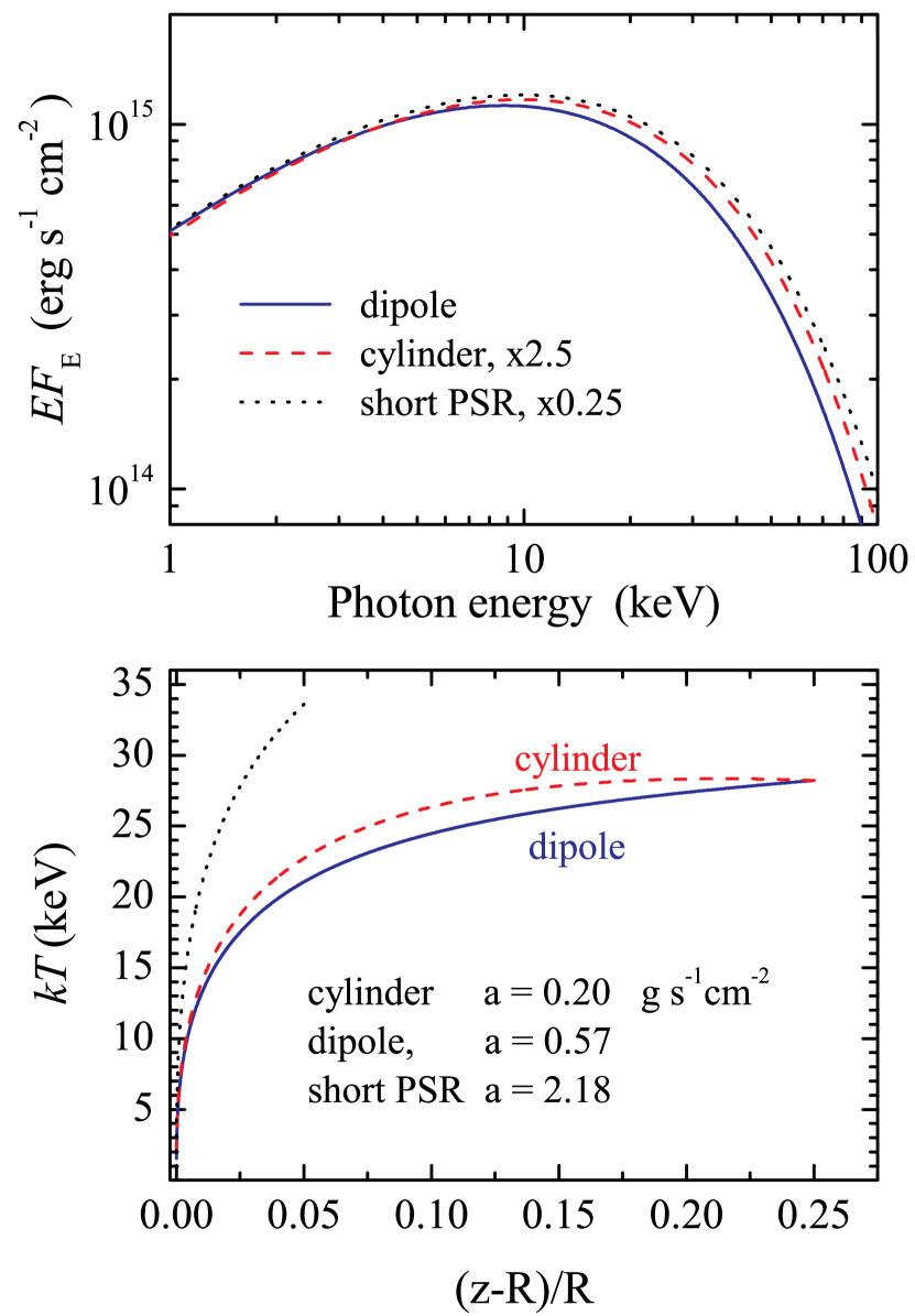
Figure 1: Comparison of model spectra (top panel) and temperature structures (bottom panel) of short and tall PSRs. The tall PSR model is computed for two geometries (cylinder and dipole).

In our previous work (Suleimanov et al., 2016) we only considered the case of high accretion rates, which is relevant for most IPs. However, the respective model grid could be inadequate for IPs with low luminosities where the local mass-accretion rate might be low and thus the height of the shock must be taken into account. For instance, the closest known IP, EX Hya, has a very low luminosity, $L\approx 10^{32}$ erg s^-1 cm^-2, see, e.g., Suleimanov et al. (2005). Recently Luna et al. (2018) concluded that the PSR in this IP could indeed be tall enough to affect the spectrum. As we will discuss below, the situation is similar for several other sources, so we extend the model presented in Suleimanov et al. (2016) also to low accretion rates.

Given the uncertainties in our knowledge of the local accretion rates, we only computed a single two-parameter model grid for fixed $H_{\rm sh}/R=0.25$, which corresponds to the tall-column limit. We considered WD masses $m=M/$M_⊙ from 0.3 to 1.2 equidistantly distributed within this range with a step of 0.02. The magnetospheric radius is expressed in units of the WD radius, $r_{\rm m}=R_{\rm m}/R$ and changes as $60/N$, where $N$ takes values from 1 to 40. In addition we computed models for very large $r_{\rm m}=1000$ to simulate accretion from infinity. Details of our model computations are described in Suleimanov et al. (2016). The main feature of the method is using a quasi-dipole geometry of the PSR as suggested by Hayashi & Ishida (2014a). Effectively we assume that the PSR cross-section increases with height above the WD surface (defined along the vertical coordinate $z$) as $S=(1+z/R)^{3}$ (Hayashi & Ishida, 2014a). The only difference between our models presented earlier and here is, thus, the assumed local mass-accretion rate. In Suleimanov et al. (2016) we fixed the total mass-accretion rate to $\dot{M}=10^{16}$ g s^-1 and the fraction of the WD surface occupied by the PSR to $f=S_{\rm PSR}/4\pi R^{2}=5\times 10^{-4}$. The local accretion rate $a$ was then adjusted to match these values for given WD mass and radius. In contrast, here we consider the tall-column limit and fix the PSR height to $H_{\rm sh}/R=0.25$, again adjusting the local accretion rate $a$ to match this value for given WD mass and radius.

The impact of increased accretion-column height on temperature structure and emerging spectrum is illustrated in Fig. 1. As expected, the spectrum of a tall PSR is softer than that of a short PSR. This effect is more significant for a PSR model assuming quasi-dipole geometry in comparison with a PSR model with simple cylindrical geometry. The reason is that the density of the model computed in quasi-dipole geometry is higher, which increases the cooling rate compared to the cylindrical model.

Speaking of cooling, it is important to emphasize that while we use an accurately computed cooling function to calculate the PSR structure, only free-free emission assuming the full ionization of 15 chemical elements is used to calculate the emerging spectra (see details in Suleimanov et al., 2016). Therefore, the models underestimate the bolometric fluxes compared to actual PSR luminosities. Quantitatively, this reduction slightly depends on the assumed magnetosphere size and mass of the WD, and as a result the model spectra give bolometric luminosities of about 70–80% of the total PSR luminosities. This does not affect shape of the spectrum or derived WD mass, because almost all the missing radiation escapes below 3 keV, but it is important for estimates of the accretion rate based on the observed flux.

3 Observations and data analysis

To confront models with observations, we opted to use two data sets. The first consists of dedicated IP observations carried out by the NuSTAR observatory either individually, or in the framework of the currently ongoing legacy survey for IPs. In the range 20–80 keV, NuSTAR has the highest sensitivity of all past and currently operating facilities, and thus is particularly well suited for studies of faint sources, such as WD mass measurements. The IPs observed by NuSTAR together with effective exposure times are listed in Table 1 (see also Table 2). To complement the NuSTAR dataset we used IP spectra provided by the Swift/BAT 105-Month Hard X-ray Survey (Oh et al., 2018). Despite the lower sensitivity, long cumulative exposure across the entire sky allowed to significantly increase the sample of considered sources. It is worth noting that spectra in this dataset are integrated over a 105 months period, so the results are not really meaningful for transient sources like GK Per, where dedicated observations are required. The IPs from the Swift/BAT Survey considered in this work are listed in Table 3.

Table 1: List of IPs observed by NuSTAR and considered in this work. Effective exposures times after standard screening are also listed.

Name	Obs. id	Exposure, ks
NY Lup	30001146002	23
EX Hya	30201016002	25
V2731 Oph	30001019002	49
GK Per	90001008002	42
	30101021002	72
TV Col	30001020002	50
V1223 Sgr	30001144002	20
V405 Aur	30460007002	38
RX J2133+5107	30460001002	26
FO Aqr	30460002002	26
V709 Cas	30001145002	26

As already mentioned in the introduction, many IPs have rather complex spectra below 10 keV either due to the presence of a partial covering absorber or due to reflection. While we have found that it is possible to adequately describe broadband NuSTAR spectra in the 3–80 keV range with PSR models in combination with either a partial covering absorber or a reflection component, or both (see also Shaw et al., 2018), we found also that fit results including the deduced WD mass are dominated in this case by the soft band, where most photons are detected, and thus strongly affected by the quantitative description of the absorption/reflection modifying the PSR spectrum. On the other hand, the WD mass in the model is effectively defined by the high-energy rollover which is generally above 20 keV. Given that no robust description of the absorption/reflection exists, we chose, therefore, to restrict the analysis to $E>20$ keV for NuSTAR and $E>15$ keV for Swift/BAT, where the contribution of these effects are less important. The advantage of this approach is that a much simpler model can be used to describe the spectra in this case. In particular, we only use a PSR model component, which in the end implies that final statistical uncertainties for the derived WD parameters are comparable to the case when the entire energy band is described with a more sophisticated model. Another advantage is that we can also directly compare results obtained with both instruments as they effectively operate in same energy range.

For the reduction of the Swift/BAT data, we used survey-averaged response files, and assigned conservative 10% model systematics for all sources to account for deviations from the model observed in first energy bin of some objects, presumably due to absorption/reflection which might be still significant in 15–20 keV band (see also Shaw et al., 2018). We opted for this approach to ensure that an acceptable fit can be achieved for all objects in a uniform way.

The reduction of the NuSTAR data was carried out using the heasoft 6.24 package and current calibration files (v20180814). The source spectra were extracted for each of the two NuSTAR modules independently from source-centered regions with radius of 45–80^′′. The extraction radius was optimized individually for each source in order to achieve best signal-to-noise ratio in the 20–80 keV band. Background spectra were extracted from the adjacent source-free regions for each observation. All spectra were grouped to contain at least 25 source counts per energy bin. For each observation the spectra were extracted and modeled for both NuSTAR modules independently, with all fit parameters except normalization linked for both modules. No systematic error was included in this case. Note that for plotting we combine the data from both NuSTAR units, and group the combined spectra to contain at least 100 counts per energy bin to enchance the clarity of the figures.

We have also carried out a timing analysis for all IPs observed by NuSTAR with the aim to detect the break in the aperiodic power spectrum and to constrain the break frequency. To increase counting statistics, light curves with time bin of 10 s in the full 3–80 keV band were extracted, with light curves from the two modules co-added. The light curves were then corrected to the solar barycenter. No background subtraction was done because background is negligible in this case, and furthermore, not relevant for the timing analysis. Besides the aperiodic variability, IPs exhibit also coherent pulsations which need to be subtracted prior to modeling of the aperiodic power spectrum. To subtract the pulsations, we followed the procedure suggested by Revnivtsev et al. (2009b). For each observation we first obtained average folded pulse profiles using the spin periods from literature (see Table 3) and the heasoft task efold. Using the same folding parameters, we then calculated the pulse phase for each light curve time bin, and subtracted the expected average rate for the respective time bin, which effectively suppresses pulsations. The power spectra were then obtained using the task powspec and binned logarithmically.

For the sources where a break in the aperiodic power spectrum was detected, we converted the obtained power spectrum into a format readable by Xspec using the heasoft task flx2xsp (see also Ingram & Done, 2012). Power spectra were then modeled together with the energy spectra using a broken power-law model with the break frequency linked to the magnetospheric radius parameter in PSR model, assuming that the break corresponds to the Keplerian frequency at this radius.

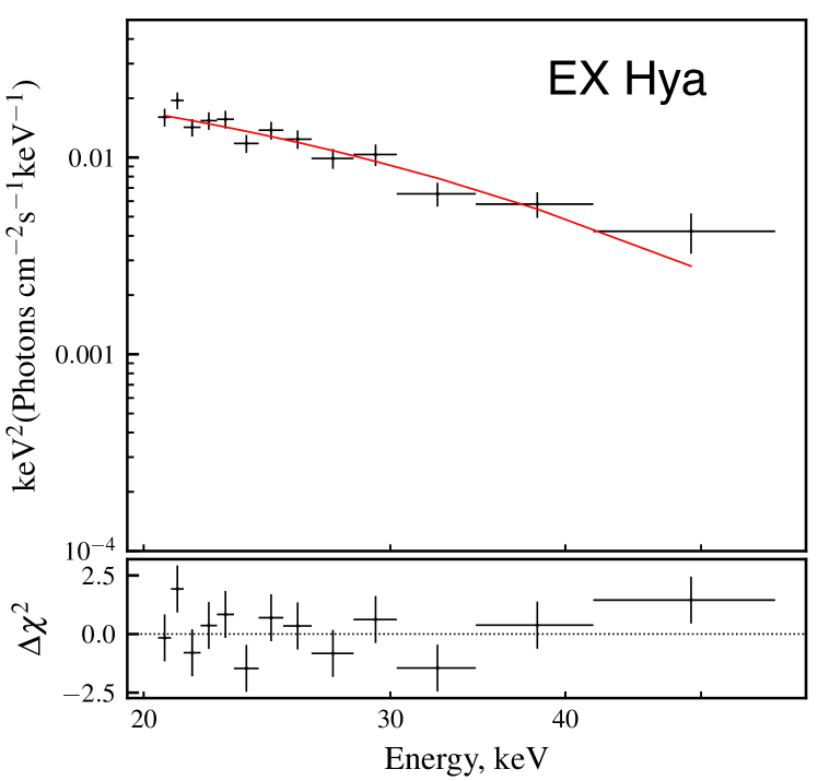
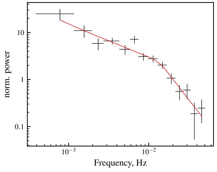
Figure 2: Top panel: NuSTAR spectrum of EX Hya fitted by a tall PSR model ($M=0.70$ M_⊙ and $R_{\rm m}=3.4\,R$) together with residuals of the fit. Spectra from both NuSTAR units combined for plotting to enhance clarity. Bottom panel: the power spectrum of EX Hya fitted with a broken power law, $\nu_{\rm br}=0.013$.

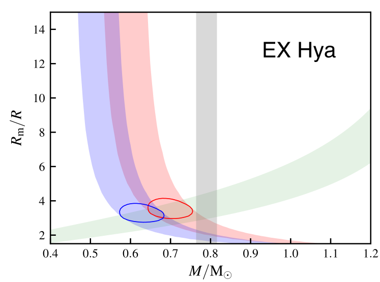
Figure 3: Strips in the $m-r_{\rm m}$ plane obtained using spectral fitting by short (blue strip) and tall (red strip) PSR models, and using the break frequency $\nu_{\rm br}=0.013$  Hz in the power spectrum of EX Hya (green strip). The corresponding most probable regions are shown by the solid closed curves. The vertical strip corresponds to the WD mass derived from optical observations.

3.1 NuSTAR observations of EX Hya

As already mentioned, there is an intrinsic degeneracy of WD mass and height from which the accretion flow starts to fall freely, i.e. the magnetosphere radius. Therefore, the magnetosphere size must be estimated independently. The simplest assumption one can make is to assume that a given WD is close to corotation, i.e., the magnetospheric radius is equal to the corotation radius

$$R_{\rm m}\simeq R_{\rm c}=\left(\frac{GMP_{\rm spin}^{2}}{4\pi^{2}}\right)^{1/3}$$ (3)

where $P_{\rm spin}$ is spin period of the WD. This assumption is likely well justified for persistent sources, or transients in quiescence, but must clearly be violated in some cases, most notably for transients during outburst.

At higher accretion rates the magnetosphere is compressed by the accretion flow. The size of the magnetosphere is defined mostly by the magnetic field strength and accretion rate in this case. Revnivtsev et al. (2009b) demonstrated that observed power spectra of the stochastic variability in accreting systems with magnetized compact objects exhibit a break at frequencies close to the compact object’s spin period. Furthermore, the frequency of the break was found to be correlated with the accretion rate, and comparable to the expected Keplerian frequency at the magnetosphere radius.

Later Revnivtsev et al. (2010) and Revnivtsev et al. (2011) used this fact to estimate the magnetospheric radius in several IPs. In particular, they found the break frequency for EX Hya, $\nu_{\rm br}=0.021\pm 0.001$ Hz (Revnivtsev et al., 2011), which corresponds to a magnetospheric radius of $R_{\rm m}\approx 2.7R$ assuming that the break frequency equals the Kepler frequency at the magnetospheric radius and a WD mass of 0.79 M_⊙ deduced from optical measurements (Beuermann & Reinsch, 2008).

Generally the WD mass is unknown and the measured break frequency only constrains a region in the $m-r_{\rm m}$ plane

$$\nu_{\rm br}=\sqrt{\frac{GM}{2\pi R^{3}_{\rm m}}}.$$ (4)

The intersection of this region with the region obtained through X-ray spectrum fitting can then be used to estimate both mass and magnetospheric radius of a given WD simultaneously. We applied this approach to obtain parameters of two IPs, EX Hya and GK Per (Suleimanov et al., 2016). For EX Hya, using Suzaku data, we found the break frequency $\nu_{\rm br}=0.021\pm 0.006$ Hz, which together with spectral modeling yielded $M=0.73\pm 0.06$ M_⊙ and $R_{\rm m}=2.6\pm 0.4\,R$. These values are in good agreement with estimates obtained by other authors (see references above). Given that GK Per was observed in two luminosity states, we also investigated the dependence of the magnetosphere radius on luminosity.

Later on, EX Hya has been also observed by NuSTAR (Luna et al., 2018). Here we use this observation to verify the results obtained previously as well as the hypothesis that the height of the PSR might be sufficiently large to affect its spectrum (Luna et al., 2018). Compared to Suleimanov et al. (2016), we also use the improved method to merge the two constraints. Instead of fitting an observed spectrum and power spectra independently and then determining the intersection between the constraints provided by both measurements on the $m-r_{\rm m}$ plane, we now fit both the energy and power spectra simultaneously. The break frequency is not considered as a free parameter but instead is linked to the $R_{m}$ parameter in the PSR model, assuming that the break occurs at the Keplerian frequency for a given radius, i.e. using Eq. 4 and 6. This approach allows to properly take the statistical uncertainties for both energy and power spectra into the account, and to directly evaluate the intersection region in the $m-r_{\rm m}$ plane.

The results are presented in Figs. 2 and 3. The best fit to the observed energy spectrum and power spectrum is shown in Fig. 2. Only the fit obtained with the tall PSR model is shown because the difference between the fits obtained for both model grids is negligible and only the derived mass is slightly different. This difference is illustrated in Fig. 3. Unlike most of the plots, we adopt a $3\sigma$ confidence level to emphasize the significance of the difference between the two model grids. It is also clear that results of the fitting with the tall PSR models better agree with the optical measurement of the WD mass. Therefore, we confirm the suggestion by Luna et al. (2018) that a tall PSR in EX Hya might be the reason behind the discrepancies between different mass estimates previously reported. The WD mass and the magnetospheric radius deduced using the tall PSR model are $0.70\pm 0.04$ M_⊙ and $3.4^{+0.4}_{-0.3}R$. Note that EX Hya might have an even taller PSR than assumed in the tall column model, $H_{\rm sh}/R=0.25$.

The distance to EX Hya is known with high accuracy after Gaia DR2. After conversion of the measured parallax we obtained $D=56.95\pm 0.13$ pc. Therefore, the mass accretion rate in the system can be deduced using the bolometric flux measured by NuSTAR. The best fit model flux is estimated to $F_{0.1-100}=1.93\times 10^{-10}$ erg s^-1 cm^-2. According to our computations the bolometric flux of this model is about 70% of the total luminosity, and the corresponding correction factor is $C\approx 1.43$. We used both the WD mass and the magnetospheric radius to derive the mass-accretion rate using the relation

$$C\times F_{0.1-100}=\frac{GM\dot{M}}{4\pi D^{2}}\left(\frac{1}{R}-\frac{1}{R_{\rm m}}\right).$$ (5)

We obtained $\dot{M}\approx 1.3\times 10^{15}$ g s^-1 (or $\approx 2\times 10^{-11}$ M_⊙/yr). Here we employed the mass-radius relation for WDs from Nauenberg (1972):

$$R=7.8\times 10^{8}\left[\left(\frac{1.44}{m}\right)^{2/3}-\left(\frac{m}{1.44}\right)^{2/3}\right]^{1/2}{\rm cm}.$$ (6)

The uncertainties in $M$ and $R_{\rm m}$ almost cancel each other, and only the uncertainty in the distance is important, which is small in our case. The derived luminosity of EX Hya is thus $L\approx 7.5\times 10^{31}$ erg s^-1.

Formally, the evaluated mass-accretion rate is so low that EX Hya, having an orbital period of $P_{\rm orb}=1.638$ h, already enters the region occupied by post-period-minimum CVs according to theoretical expectations for the $\dot{M}-P_{\rm orb}$ relation (see, e.g. Howell et al., 2001; Goliasch & Nelson, 2015). On the other hand, the recently measured secondary mass $M_{2}=0.10\pm 0.02$ M_⊙ (Echevarría et al., 2016) excluded this possibility. Therefore, EX Hya is just a system in a low-accretion state. Indeed, Vogt et al. (1980) (see also Bateson et al. 1979) remarked that EX Hya is a dwarf nova with very short duration ($\approx\,4^{\rm d}$) and rare (every 574^d) outbursts. Our result supports this statement.

Using the determined mass-accretion rate we can also evaluate the magnetic field strength $B$ on the WD surface. Assuming that the magnetospheric radius is proportional to the standard Alfvén radius $R_{\rm m}=\Lambda R_{\rm A}$, we get

$$r_{\rm m}=\frac{R_{\rm m}}{R}=\Lambda\left(\frac{B^{4}R^{5}}{2GM\dot{M}^{2}}\right)^{1/7},$$ (7)

or

$$B=(2GM)^{1/4}\,\dot{M}^{1/2}R^{-5/4}\left(\frac{r_{\rm m}}{\Lambda}\right)^{7/4}.$$ (8)

Inserting numerical values, this implies $B=2.9\times 10^{4}$ G assuming that $\Lambda=0.5$. This low value is, however, slightly higher in comparison with previous results (see, e.g., Revnivtsev et al., 2011).

3.2 NuSTAR observations of GK Per

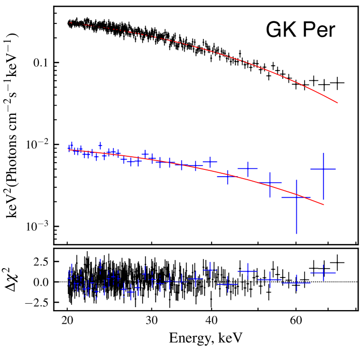
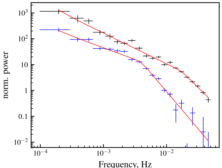
Figure 4: Top panel: NuSTAR spectra of GK Per during outburst and quiescence fitted with short PSR models ($M=0.79$ M_⊙, $R_{\rm m}=3.18\,R$ for outburst and $R_{\rm m}=8.5\,R$ in quiescence). Spectra from both NuSTAR units combined for plotting to enhance clarity. Bottom panel: The corresponding power spectra fitted with broken power laws, $\nu_{\rm br}=0.017$ (outburst) and $\nu_{\rm br}=0.004$ (quiescence).

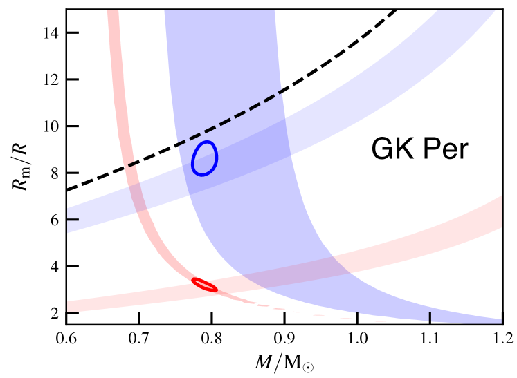
Figure 5: Strips in the $m-r_{\rm m}$ plane obtained using spectral fitting of GK Per during outburst (red strips) and quiescence (blue strips) by short column PSR models, and using the break frequency in the power spectrum during outburst ($\nu_{\rm br}=0.017$ Hz) and quiescence ($\nu_{\rm br}=0.004$ Hz). The corresponding most probable regions are shown by the solid closed curves. The dashed curve corresponds to the corotation radius.

The old nova GK Per is an IP which exhibits dwarf nova behavior as well (Watson et al., 1985; Šimon, 2002). Therefore, the states of the system with the very different accretion rates are observed, so the magnetospheric radius in this system is expected to differ in quiescence and outburst. We attempted to investigate whether this is indeed the case (Suleimanov et al., 2016) using a NuSTAR observation of GK Per during the latest outburst (Zemko et al., 2017), and Swift/BAT and INTEGRAL hard X-ray spectra of the source in quiescence. This allowed to estimate the magnetosphere size respectively using observed break frequency, and from PSR model under assumption that the mass of WD is the same in both cases. No dedicated observations of the source quiescence were available at the time (Wada et al., 2018) so we were not able to investigate the power spectrum. Note that Wada et al. (2018) used a similar approach to study the magnetospheric radius changes, but they employed another spectral model, and obtained consistent results. In particular, they derived a WD mass of $0.87\pm 0.07$ M_⊙ which is in very good agreement with our result $0.86\pm 0.02$ M_⊙.

A NuSTAR observation of GK Per in quiescence became available since then, and this dataset allows us to directly measure the power spectrum of the source. Its shape is similar to that during the outburst, and the break is clearly detected. The break occurs at significantly lower frequency, as expected. This is illustrated in Figs. 4 and 5. The best fits to the GK Per spectra and power spectra during outburst and quiescence are shown in Fig. 4. Again, we fit both power and energy spectra simultaneously as described above for EX Hya, with break frequencies in outburst and quiescence linked to the respective $R_{m}$ parameter values of the PSR model. The mass of the WD was linked for both data sets. The results are presented in Fig. 5. The contours for the WD mass and magnetosphere size for the two states obtained from the joint fit are shown by solid curves. For illustration we also plot the constraints which are obtained by independent fitting of energy and power spectra (as colored strips in the plot). From the joint fit we obtain $M=0.79\pm 0.01$ M_⊙ and $R_{\rm m}/R=3.18\pm 0.17$ (at outburst) and $R_{\rm m}/R=8.5\pm 0.5$ (at quiescence). The obtained WD mass and magnetospheric radii are slightly reduced compared to our previous result. The reason for that is most likely related to the fact that GK Per is a transient system, so the mission-long Swift/INTEGRAL spectra used previously to determine WD parameters in queiscence contain also some outburst data. We also note that the magnetospheric radius in quiescence is close to the corotation radius.

The distance to GK Per is now constrained by Gaia DR2 to $D=442\pm 8.5$ pc. This allows to estimate the mass-accretion rates and corresponding luminosities during outburst ($7.87\times 10^{17}$ g s^-1 and $5.8\times 10^{34}$ erg s^-1) and in quiescence ($1.42\times 10^{16}$ g s^-1 and $1.4\times 10^{33}$ erg s^-1). The corresponding magnetic field strengths on the WD surface are $B\approx 7.5\times 10^{5}$ G and $B\approx 5.6\times 10^{5}$ G. This difference indicates that the magnetospheric radius dependence on accretion rate deviates slightly from one expected from Alfvén model. Indeed, one would expect that the ratio of the magnetospheric radius in quiescence $R^{q}_{\rm m}$ to the measured one during outburst $R^{o}_{\rm m}$ has to be proportional to the mass-accretion rates:

$$\frac{R^{q}_{\rm m}}{R^{o}_{\rm m}}\sim\left(\frac{\dot{M}^{q}}{\dot{M}^{o}}\right)^{-2/7}\approx 3.15\pm 0.05.$$ (9)

The observed ratio is $2.7\pm 0.21$, i.e., the discrepancy between the two values is $\sim$ 2$\sigma$. Wada et al. (2018) obtained a higher ratio, $3.9\pm 0.5$, with systematically smaller measured magnetospheric radii (based on spectral fits only).

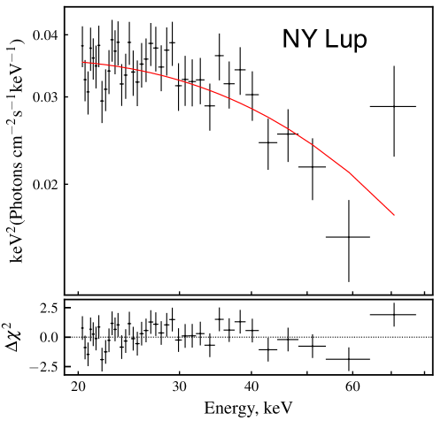
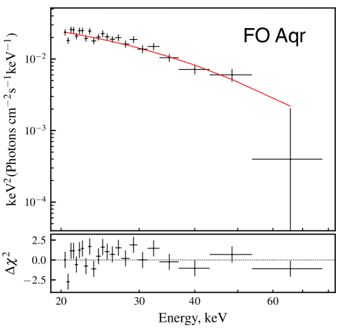
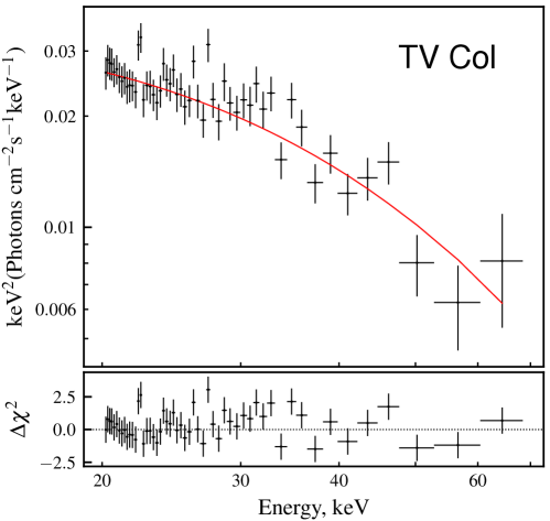
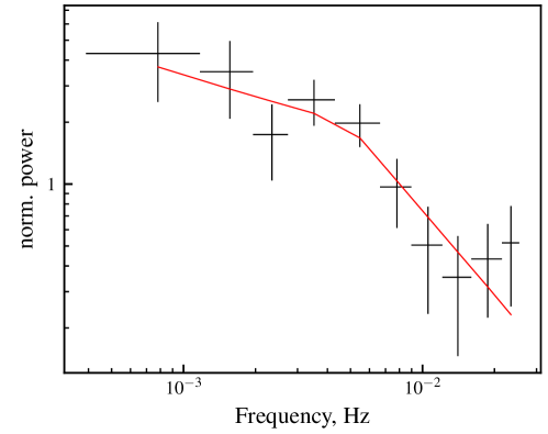
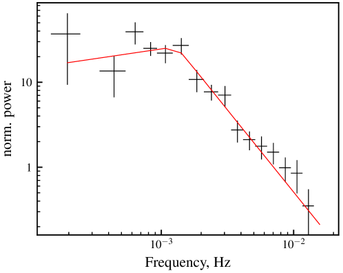
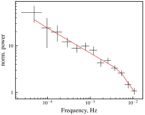
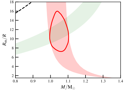
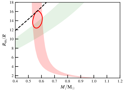
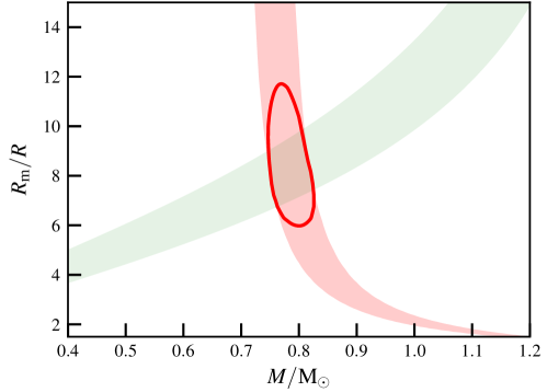
Figure 6: Top panels: NuSTAR spectra of NY Lup, FO Aqr, and TV Col fitted with short PSR models. Spectra from both NuSTAR units combined for plotting to enhance clarity. Middle panels: The corresponding power spectra fitted with broken power laws. Bottom panels: Strips in the $m-r_{\rm m}$ plane obtained using spectral fitting (red strips) by short column PSR models, and using the break frequency in the power spectra (green strips). The corresponding most probable regions are shown by the solid closed curves. The dashed curves correspond to the corotation radii. The used fitting parameters are presented in Table 2.

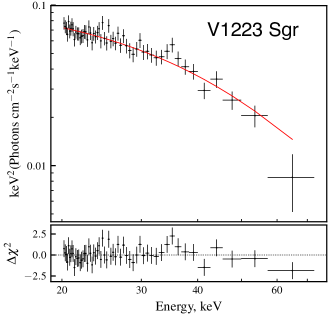
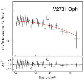
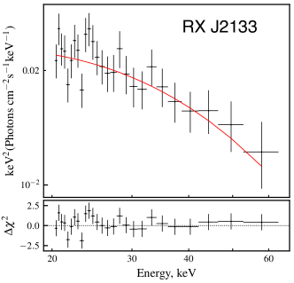
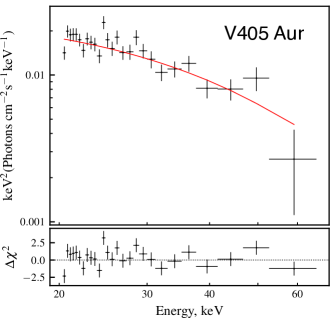
Figure 7: NuSTAR spectra of V709 Cas, V1223 Sgr, V2731 Oph, RX J2133, and V405 Aur fitted with short PSR models. Spectra from both NuSTAR units combined for plotting to enhance clarity. The used fitting parameters are presented in Table 2.

Table 2: Observed and derived parameters of IPs observed by NuSTAR.

Name	$M/$M⊙	$\nu_{\rm br}$, Hz	$R_{\rm m}/R$	$F^{b}_{0.1-100}$
GK Per	$0.79\pm 0.01$	0.017	3.18 $\pm$0.17	24.79$\pm$0.5
		0.004	8.5${}^{+0.5}_{-0.4}$	0.59$\pm$0.03
NY Lup	$1.05\pm 0.04$	0.005	10.3${}^{+2.8}_{-2.0}$	2.08$\pm$0.11
FO Aqr	$0.57\pm 0.03$	0.0013	14.1$\pm$1.1	2.38$\pm$0.31
V2731 Oph	$1.06\pm 0.03$		7.8a	1.47$\pm$0.07
V709 Cas	$0.83\pm 0.04$		9.6a	1.57$\pm$0.14
EX Hya	$0.70\pm 0.04$	0.013	3.4${}^{+0.4}_{-0.3}$	1.93$\pm$0.42
V1223 Sgr	$0.72\pm 0.02$		14.4a	5.39$\pm$0.32
V405 Aur	$0.73\pm 0.03$		12.0a	1.31$\pm$0.14
J2133+5107	$0.95\pm 0.04$		17.2a	1.35$\pm$0.09
TV Col	$0.79\pm 0.03$	0.005	7.6${}^{+2.6}_{-1.2}$	1.87$\pm$0.12

Notes: (a) Relative corotation radius; (b) Best fit model flux in the range 0.1–100 keV in units $10^{-10}$ erg s^-1 cm^-2.

3.3 Other intermediate polars observed with NuSTAR

Up to now, observations of ten IPs were performed by NuSTAR, and we applied the approach described in detail above to all of them. The available data does not always allow to obtain a power spectrum with sufficient quality, particularly for slower rotating sources, and thus to detect the break. The magnetospheric radii were estimated, therefore, using the break frequency whenever possible, or fixed to the corotation radius otherwise. The results are presented in Table 2 and Figs. 6 and 7.

Masses of three IPs (NY Lup, V1223 Sgr, and V709 Cas) were determined by Shaw et al. (2018) using NuSTAR observations. The reported values are $1.16^{+0.04}_{-0.02}M_{\odot}$, $0.75\pm 0.02M_{\odot}$, and $0.88^{+0.05}_{-0.04}M_{\odot}$, respectively. Comparison with our estimates suggests that we obtain slightly smaller masses. There are several possible reasons for this discrepancy.

First of all, we restrict our analysis to the energy range above 20 keV due to the apparent complexity of the spectrum at lower energies which is not accounted for by the model. While it is clear that reflection or complex absorption must be responsible for the observed deviations from PSR model, as already discussed above, there is no physically motivated quantitative description of these deviations, yet (see, however, Hayashi et al., 2018). Shaw et al. (2018) considered the full NuSTAR energy range and concluded that reflection is essential to describe the broadband spectrum. However, a rather simplified description for the reflection component was necessarily used, which could bias their estimates. Indeed, the overall fit quality and thus estimated properties of the reflection component are dominated by the soft band. On the other hand, the reflection bump peaks around 20–40 keV (Magdziarz & Zdziarski, 1995), i.e., close to the expected rollover of the PSR spectrum. As a consequence, the rollover energy ultimately defining the estimated WD mass, becomes strongly dependent on the ad-hoc description of the soft part of the spectrum, which is clearly not desirable. We thus restricted the analysis to the energy range which, from a physical point of view, gives a real constraint for the parameter of interest, i.e., the WD mass.

Note that Hailey et al. (2016) also estimated WD masses for two IPs observed with NuSTAR, namely TV Col and V2731 Oph. They used an approach similar to ours and for the same reasons restricted their analysis to the $\ >15$ keV energy range. As a result, they found masses of $0.77\pm 0.03$ M_⊙ and $1.16\pm 0.05$ M_⊙ respectively, which are close to our estimates for these sources.

It appears also that the difference between our results and those obtained by other authors is more significant for heaviest WDs. We believe that the reason for this is the use of the different models of the PSR. Hailey et al. (2016) and Shaw et al. (2018) used the models computed by Suleimanov et al. (2005) in cylindrical geometry for a fixed local mass-accretion rate $a=1$ g s^-1. This value is comparatively low and implies a tall PSR for heavy WDs. As a result, the maximum PSR temperature in such models is lower than the maximum temperature in the case of a short PSR, and a more massive WD is required to reproduce the observed spectrum. On the other hand, our model spectra (Suleimanov et al., 2016) are computed for a fixed $\dot{M}=10^{16}$ g s^-1 and relative PSR footprint area $f=5\times 10^{-4}$. Under these conditions the local mass-accretion rate increases with the WD mass so that the PSRs remain short for any WD mass, i.e., our model is self-consistent. For low-luminosity IPs, where the PSR might indeed be tall, a separate model grid must be used to avoid a bias in the WD mass determination.

4 Swift/BAT observations

While NuSTAR provides data of exceptional quality, the number of dedicated observations is limited. To increase the sample of objects, we used, therefore, also the energy spectra accumulated throughout the Swift mission lifetime, as mentioned above. The Swift/BAT spectra cover the energy range above 15 keV, so the results shall be comparable with those obtained with NuSTAR. We have identified 35 sources significantly detected in the Swift/BAT Survey and known as IPs. The final list of objects can be found in Table 3. As no timing is available for most objects, we assumed corotation ($R_{\rm m}=R_{\rm c}$) in these cases. We considered also both, short and tall PSR models for all objects, and list the fit results for the tall PSR where observed flux and estimated distance indicate this model might be better justified.

Note that we excluded GK Per and EX Hya from the comparison because the assumption that the matter falls from the corotation radius is clearly inapplicable for these objects. As illustrated in Fig. 8, the results obtained for NuSTAR and Swift/BAT are otherwise broadly compatible for the objects observed by both observatories, as expected. Inclusion of the Swift/BAT data allows, however, to significantly increase the source sample, to compare our results with previous investigations, and to assess how various theoretical uncertainties might affect the deduced WD masses for the entire population.

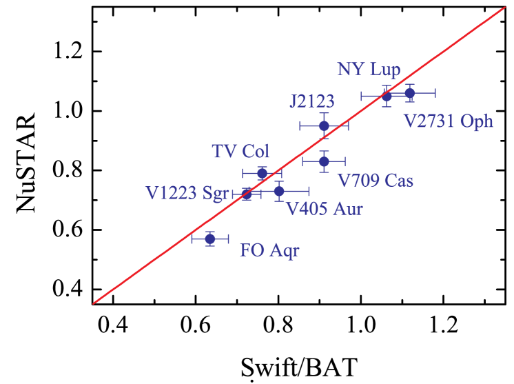
Figure 8: Comparison of the WD masses obtained by fitting their spectra observed by NuSTAR and Swift/BAT.

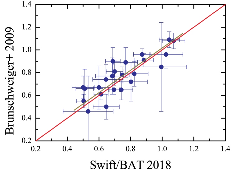
Figure 9: Comparison of the WD masses obtained by Brunschweiger et al. (2009) and by us.

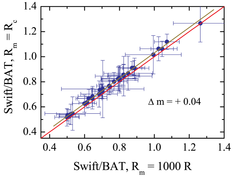
Figure 10: Importance of the finite magnetospheric radii for WD mass determination.

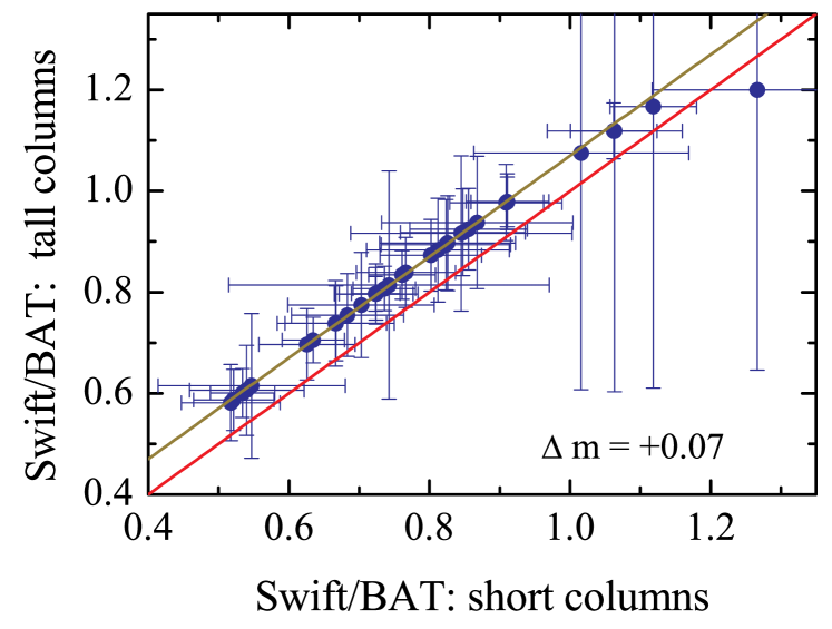
Figure 11: Systematic difference between WD masses derived with using short and tall PSR models.

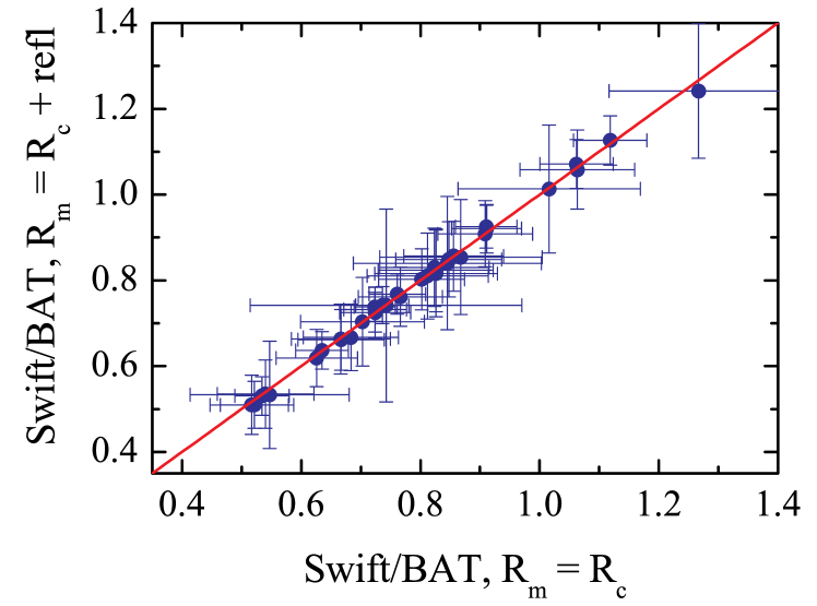
Figure 12: Difference between WD masses derived using short PSR models with and without reflection component taken into account.

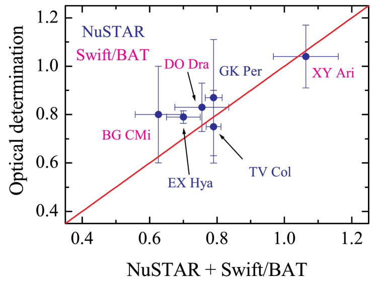
Figure 13: Comparison of the WD masses derived from X-ray spectra and obtained by optical methods.

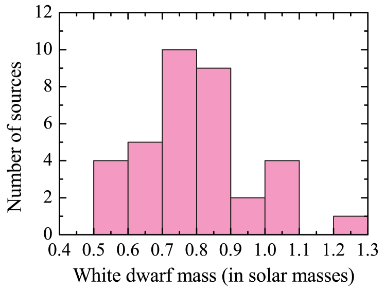
Figure 14: Distribution of WD numbers over their masses.

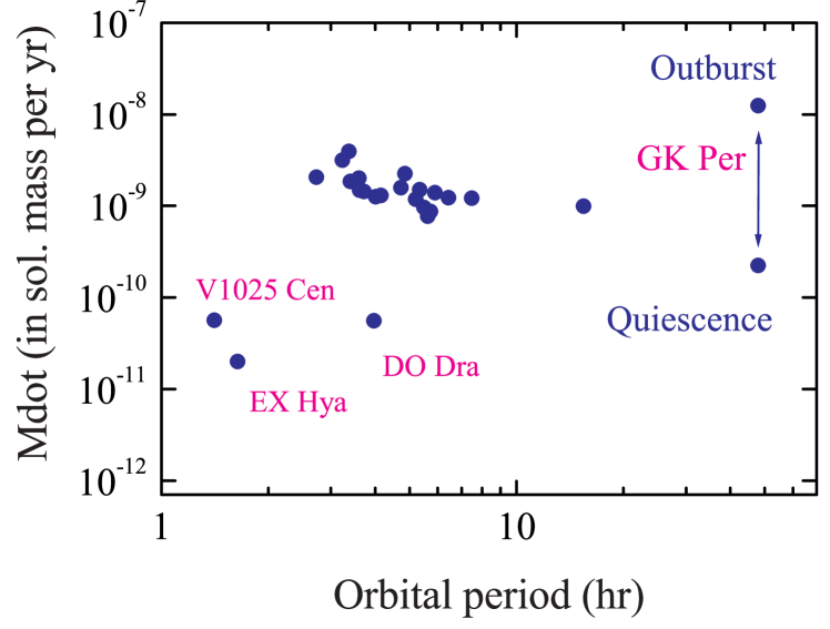
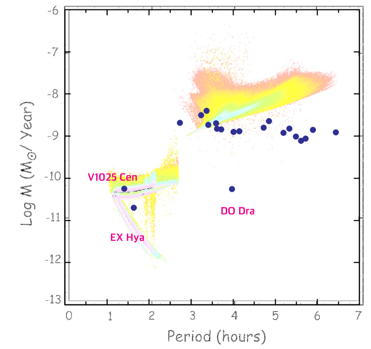
Figure 15: Distribution of mass-accretion rates in the studied IPs vs. orbital periods. Top panel: Only IPs with Gaia DR2 distances $<$1 kpc are shown. Bottom panel: Same results together with model predictions by Howell et al. (2001); © AAS; reproduced with permission.

Figure 16: Distribution of WD magnetic field strengths in the studied IPs vs. orbital periods. Only IPs with the Gaia DR2 distances $<$1 kpc are shown.

5 Intermediate polar statistics

5.1 Comparison with published works and consistency checks

First of all, we compare WD masses obtained by Brunschweiger et al. (2009) (23 IPs) with those found by us for the same sources and using the same assumptions (Fig. 9). In particular, for this comparison we used the short PSR models with the fixed relative magnetospheric radius $R_{\rm m}=1000\,R$ because Brunschweiger et al. (2009) used our old models (Suleimanov et al., 2005) computed in cylindrical geometry assuming matter falling from infinity. Fig. 9 demonstrates that under this approximation the difference between the old model grid and the new one with a more realistic PSR cross-section is minor, and the results are consistent within uncertainties.

We can now move one step further, and repeat the analysis using the same model grid, but fixing the relative magnetospheric radii to the corotation ones, which is more realistic. The comparison of the obtained WD masses with those found using the assumption about matter falling from infinity is presented in Fig. 10. The new masses are shifted to larger values, and the average displacement for the sample is about $+0.04M_{\odot}$, which is comparable with the typical uncertainty in the WD mass determination. The conclusion one could make is that on average IPs are sufficiently close to corotation to make the resulting difference in spectral shape for the two assumptions undetectable in available data. Note, however, that this might not hold for dedicated pointed observations.

Another source of uncertainty is the assumed PSR height. We repeat the analysis for all 35 sources using the new tall PSR model, again assuming corotation. As expected, the results are shifted to higher WD masses and the shift amounts to $+0.07M_{\odot}$ (Fig. 11). The statistical uncertainties of the massive WDs measured using the new grid are large, but this is just a consequence of the lower upper limit ($1.2M_{\odot}$) of computed WD masses in the tall PSR model grid. This is most noticeable for the massive IP IGR J08390$-$4833.

We also investigated how the reflection component might bias our mass estimates if only the hard X-ray band is considered. In particular, we repeated the above analysis assuming a short PSR, but including a reflection component reflect with the maximum possible reflection parameter $Refl=\Omega/2\pi=1$ (here $\Omega$ is the solid angle of the reflecting slab as seen from the X-ray source). As illustrated in Fig. 12, the presence of reflection does not affect the deduced masses. This confirms that our approach of relying on hard X-ray data only is indeed justified.

5.2 Statistical properties of the IP sample

Now let us discuss the statistical properties of the entire sample. We have determined the WD mass for a large number of IPs using the same model and employing an individual approach to some better investigated sources (see previous sections). The WD masses obtained using NuSTAR observations have higher accuracy, and also give a better understanding of the actual magnetosphere size, so we prefer them whenever available (see Table 2). For the rest of the objects we use the most recent Swift/BAT results. Consequently, we have now a uniform sample of WD masses in 35 IPs. The final results for all objects are summarized in Table 3. The uncertainties in the mass accretion rates $\dot{M}$, the luminosities $L$, and the magnetic field strength $B$ were estimated taking only the uncertainties in distance (the largest source of uncertainty) into account.

Table 3: Observed and derived parameters of the investigated IPs.

Name	$M/$M⊙	$P_{\rm orb}$, hr	$P_{\rm spin}$, s	$R_{\rm m}/R$	$D$, pc	$F^{b}_{0.1-100}$	$\dot{M}$, 1016g/s	$L$, 1033 erg/s	$B$, MG
EX Hya∗	0.70$\pm$0.04	1.63762	4021.62	3.4	56.95$\pm$0.13	1.93	(13$\pm$0.6)$\times 10^{-2}$	(75$\pm$0.4)$\times 10^{-3}$	(29$\pm$0.07)$\times 10^{-3}$
TV Col	0.79$\pm$0.03	5.4864	1911	7.6	512.6${}^{+4.7}_{-4.6}$	1.87	6.2$\pm$0.1	5.9$\pm$0.1	0.96$\pm$0.01
DO Dra∗	0.76$\pm$0.08	3.96898	529.3	12.2a	197.8$\pm$1.2	0.70	0.35	0.33$\pm$0.01	0.49$\pm$0.003
V405 Aur	0.73$\pm$0.03	4.14288	545.5	12.0a	675$\pm$14	1.31	8.25${}^{+0.35}_{-0.33}$	7.13${}^{+0.30}_{-0.28}$	2.2$\pm$0.05
MU Cam	0.67$\pm$0.08	4.7245	1187.22	18.2a	982${}^{+28}_{-26}$	0.66	10.06${}^{+0.58}_{-0.53}$	7.56${}^{+0.44}_{-0.40}$	4.6$\pm$0.13
V667 Pup	0.86$\pm$0.08	5.6112	512.42	13.9a	814${}^{+52}_{-46}$	0.75	4.89${}^{+0.65}_{-0.54}$	5.95${}^{+0.79}_{-0.66}$	2.7$\pm$0.2
V2400 Oph	0.72$\pm$0.05	3.408	927.6	16.8a	715$\pm$17	1.68	11.7${}^{+0.6}_{-0.5}$	10.26$\pm$0.5	4.6$\pm$0.1
BG CMi	0.63$\pm$0.07	3.23395	847.03	14.3a	993${}^{+57}_{-51}$	1.12	20.1${}^{+2.39}_{-2.02}$	13.2${}^{+1.6}_{-1.3}$	4.0$\pm$0.2
V709 Cas	0.83$\pm$0.04	5.3329	312.75	9.6a	747$\pm$12	1.57	9.6$\pm$0.3	10.5$\pm$0.3	1.9$\pm$0.03
V2731 Oph	1.06$\pm$0.03	15.42	128.1	7.8a	832${}^{+270}_{-164}$	1.47	6.3${}^{+4.8}_{-2.3}$	12.2${}^{+9.2}_{-4.3}$	1.7${}^{+0.5}_{-0.3}$
PQ Gem	0.77$\pm$0.07	5.19262	833.42	16.7a	766${}^{+22}_{-21}$	1.06	7.6$\pm$0.4	7.4$\pm$0.4	4.1$\pm$0.1
V1223 Sgr	0.72$\pm$0.02	3.36586	746	14.4a	580$\pm$16	5.39	25.1${}^{+1.4}_{-1.3}$	21.7${}^{+1.3}_{-1.2}$	5.3$\pm$0.15
AO Psc	0.53$\pm$0.05	3.59102	805.2	11.3a	495${}^{+11}_{-10}$	1.06	12.8${}^{+0.6}_{-0.5}$	6.1$\pm$0.3	1.8$\pm$0.04
V1025 Cen∗	0.61$\pm$0.14	1.41024	2146.6	24.8a	193.2${}^{+4.9}_{-4.6}$	0.52	0.36$\pm$0.02	0.23$\pm$0.01	1.4$\pm$0.03
V1062 Tau	0.81$\pm$0.10	9.98222	3780	49.1a	1582${}^{+220}_{-172}$	0.69	17.9${}^{+5.3}_{-3.4}$	20.7${}^{+6.1}_{-4.3}$	45${}^{+6}_{-5}$
XY Ari	1.06$\pm$0.10	6.06473	206.3	10.7a	2000c	0.60	14.2	28.6	4.5
FO Aqr	0.57$\pm$0.03	4.84944	1254.3	14.1	526$\pm$14	2.38	14.3${}^{+0.8}_{-0.7}$	7.9$\pm$0.4	3.0$\pm$0.1
TX Col	0.52$\pm$0.07	5.7192	1911	19.5a	512.6${}^{+4.7}_{-4.6}$	0.83	5.5$\pm$0.10	2.6$\pm$0.05	3.0$\pm$0.03
GK Per	0.79$\pm$0.01	47.9233	351.3	3.18	442.0${}^{+8.6}_{-8.3}$	24.8	78.7${}^{+3.1}_{-2.9}$	57.9${}^{+2.3}_{-2.2}$	0.75$\pm$0.1
				8.5		0.59	1.42${}^{+0.06}_{-0.05}$	1.38$\pm$0.05	0.56$\pm$0.1
V2306 Cyg	0.70$\pm$0.10	4.35708	1466.7	22.1a	1360${}^{+65}_{-59}$	0.49	13.0${}^{+1.3}_{-1.1}$	10.9${}^{+1.1}_{-0.9}$	7.8$\pm$0.4
NY Lup	1.05$\pm$0.04	9.864	693.01	10.3	1272${}^{+46}_{-43}$	2.08	20.7${}^{+1.5}_{-1.4}$	40.3${}^{+2.3}_{-2.7}$	4.9$\pm$0.2
V1033 Cas	1.02$\pm$0.15	4.032	563.5	19.2a	1554${}^{+146}_{-123}$	0.27	4.2${}^{+0.8}_{-0.6}$	7.8${}^{+1.5}_{-1.2}$	6.1${}^{+0.6}_{-0.5}$
RX J2133.7+5107	0.95$\pm$0.04	7.14	570.82	17.2a	1350${}^{+49}_{-46}$	1.35	18.7${}^{+1.4}_{-1.2}$	29.4${}^{+2.2}_{-1.2}$	9.3$\pm$0.3
V418 Gem	0.74$\pm$0.23	4.3704	480.67	11.2a	3842${}^{+4444}_{-1341}$	0.24	47.7${}^{+74.2}_{-27.5}$	42.3${}^{+155}_{-24}$	4.8${}^{+5.6}_{-1.7}$
V515 And	0.67$\pm$0.07	2.731	465.5	9.7a	1006${}^{+49}_{-44}$	0.77	13.2${}^{+1.3}_{-1.1}$	9.3${}^{+0.9}_{-0.8}$	1.8$\pm$0.08
V647 Aur	0.85$\pm$0.16	3.46656	932.9	20.4a	2251${}^{+402}_{-296}$	0.37	18.4${}^{+7.2}_{-4.5}$	22.5${}^{+8.7}_{-5.5}$	10.2${}^{+1.8}_{-1.3}$
EI UMa	0.91$\pm$0.08	6.4344	741.6	19.3a	1133${}^{+50}_{-46}$	0.72	7.8${}^{+0.7}_{-0.6}$	11.1${}^{1.0}_{-0.9}$	6.8$\pm$0.3
V2069 Cyg	0.83$\pm$0.10	7.48032	743	17.0a	1178${}^{+46}_{-43}$	0.53	7.7$\pm$0.6	8.9${}^{+0.7}_{-0.6}$	4.7$\pm$0.2
IGR J1719-4100	0.72$\pm$0.06	4.0056	1054	18.3a	654.3${}^{+17.9}_{-16.9}$	1.39	8.1${}^{+0.5}_{-0.4}$	7.1$\pm$0.4	4.6$\pm$0.1
IGR J0457+4527	0.87$\pm$0.14	7.2	1223	25.2a	4770${}^{+14891}_{-2056}$	0.48	99${}^{+1589}_{-67}$	130${}^{+2072}_{-88}$	36${}^{+112}_{-16}$
IGR J1817-2508	0.54$\pm$0.08	1.5312	1663.4	18.5a	2130${}^{+376}_{-278}$	0.92	98${}^{+38}_{-24}$	50${}^{+19}_{-12}$	11.9${}^{+2.1}_{-1.5}$
IGR J0838-4831	1.27$\pm$0.15	7.92	1480.8	65.2a	2167${}^{+327}_{-251}$	0.24	3.2 ${}^{+1.0}_{-0.7}$	13.3${}^{+4.3}_{-2.9}$	89${}^{+14}_{-10}$
IGR J1509-6649	0.85$\pm$0.09	5.8896	809.42	18.6a	1164${}^{+39}_{-37}$	0.67	8.9 $\pm$0.6	10.8$\pm$0.7	6.1$\pm$0.2
IGR J1649-3307	0.82$\pm$0.09	3.6168	571.9	14.2a	1170${}^{+91}_{-79}$	0.65	9.4 ${}^{+1.5}_{-1.2}$	10.6${}^{+1.7}_{-1.4}$	3.8$\pm$0.3
IGR J1654-1916	0.83$\pm$0.10	3.7152	546.7	14.2a	1096${}^{+62}_{-56}$	0.72	9.2${}^{+1.0}_{-0.9}$	10.4${}^{+1.2}_{-1.0}$	3.7$\pm$0.2

Notes: (a) Relative corotation radius; (b) Best fit model flux in the range 0.1–100 keV in units $10^{-10}$ erg s^-1 cm^-2; (c) Distance assumed; there is not parallax measurement of XY Ari in Gaia DR2. (*) X-ray spectra were fitted with the tall PSR models.

For some objects independent mass estimates are available, so it is interesting to compare them with our results (Fig. 13). In particular, we used mass estimates reported by Hellier (1997) for XY Ari, by Hellier (1993) for TV Col, by Haswell et al. (1997) for DO Dra, by Penning (1985) for BG Cmi, by Beuermann & Reinsch (2008) for EX Hya, and by Morales-Rueda et al. (2002) for GK Per. We note that in most cases the agreement is excellent. The largest discrepancy is observed for EX Hya where we still underestimate the mass, likely due to the fact that our tall PSR model is actually still comparatively short considering the observed accretion rate.

One could observe that Ritter’s catalog of CVs (Ritter & Kolb, 2003) includes more IPs with known WD masses. However, these estimates were also obtained using X-ray observations and methods similar to one presented here. It is not surprising, therefore, that for these objects the agreement with our estimate is perfect if the same assumptions on PSR geometry and magnetosphere size are used. We, thus, excluded these objects from Fig. 13 for clarity.

We can assess the properties of the WD mass distribution for the entire IP population presented in Fig. 14. It is consistent with being normal (p-value of $\sim$ 0.2 for Shapiro-Wilk test; Shapiro & Wilk 1965), and peaks around 0.7–0.9 $M_{\odot}$, which is consistent with past investigations (Zorotovic et al., 2011). The mean and standard deviation of WD mass in our distribution are $0.79\pm 0.16M_{\odot}$, which is close to existing estimates for CVs in general by Zorotovic et al. (2011) ($0.83\pm 0.24M_{\odot}$), and specifically for IPs by Bernardini et al. (2012) ($0.86\pm 0.07M_{\odot}$), and by Yuasa et al. (2010) ($0.88\pm 0.25M_{\odot}$). All these values are significantly larger compared to the isolated WD population with 0.6 $M_{\odot}$ (Kepler et al., 2016). There are hypotheses to explain this fact (see discussion in Wijnen et al., 2015), but their consideration is out of scope of the present work.

Gaia DR2 (Gaia Collaboration et al., 2016, 2018) opened new possibilities for IP studies. Now we have comparatively accurate determinations of the distances to many IPs (see Table 3). Therefore, their mass-accretion rates and surface magnetic fields can be estimated as described above for EX Hya and GK Per. The results are presented in Table 3. For IPs closer than 1 kpc (i.e., excluding sources with large distance uncertainties for clarity), the results are also presented in Figs. 15 and 16.

Table 4: Comparison of WD magnetic field strengths in some IPs measured from optical/IR polarization observations ($B_{\rm pol}^{a}$) with estimates obtained in the present work ($B_{\rm sp}$).

Name	$M/$M⊙	$B_{\rm pol}^{a}$, MG	$B_{\rm sp}$, MG	$R_{\rm m}/R$
NY Lup	1.05	$>$ 4	4.9	10.3
BG CMi	0.63	$\sim$ 4	4	14.3b
V2731 Oph	1.06	$\sim$ 5	1.7	7.8b
V2400 Oph	0.72	9-20	4.6	16.8b
IGR J1509 -6649	0.85	$>$ 10	6.1	18.6b
V2306 Cyg	0.70	8	7.8	22.1b
V405 Aur	0.73	32	2.2	12.0b
RX J2133+5107	0.95	$>$ 20	9.3	17.2b
PQ Gem	0.79	8-21	4.1	16.7b

Notes: (a) References to the original works with the polarization measurements can be found in Ferrario et al. (2015). (b) Relative corotation radius

It is interesting to look at the estimated mass-accretion rates as a function of orbital period to facilitate comparison with existing theoretical predictions (see, e.g. Howell et al., 2001; Goliasch & Nelson, 2015). In particular, a comparison of our result with population synthesis predictions (Fig. 15) allows to conclude that most IPs appear to have lower mass-accretion rates in comparison with the predicted values. It seems also that the observed $\dot{M}$ decreases with increasing orbital period. This behavior is opposite to the expected one, but deviation is not significant. The mass accretion rate of GK Per during quiescence is on this dependence. We can suggest that most of IPs are in a low mass accretion rate (quiescence) and might have short, rare, and barely visible outbursts. We note, however, that the mass-accretion rates of the IPs with orbital periods less than four hours are close to the modeled values. Two IPs, EX Hya and DO Dra, are in low states with observed mass-accretion rates probably less than the average values. The WD masses in these IPs were found using the tall PSR models. One short-period IP below the period gap, V1025 Cen, has a low mass accretion rate, close to the expected value. The WD mass in this IP was also determined using the tall PSR model spectra.

We compare the derived magnetic field strengths on the WD surface to the orbital periods in Fig.16. Our results range between 1 and 10 MG, although in many cases the values shall be considered as upper limits only, because we had to assume corotation for many IPs due to lack of other magnetospheric radius estimates. The actual magnetospheric radii might be smaller. The field strength in EX Hya is extremely low, and this object is probably observed as an IP only because of the extremely low mass-accretion rate, which raises the question whether we miss a significant population of similar sources which are too distant and faint for periodic variability to be detected.

There are also several IPs with WD magnetic fields stronger than 10 MG, but all of them have distances beyond 2 kpc, which are poorly constrained. As a consequence, large magnetic field values might just be due to overestimated distances.

The magnetic field strength can be also determined using optical/IR polarization measurements (see details in Ferrario et al., 2015). These authors provide a list of WDs in IPs investigated in this way. We list them in Table 4 together with our estimates. For three sources, namely NY Lup, V2306 Cyg, and BG CMi there is good agreement. On the other hand, for the rest of the sources we significantly underestimate the field strength. We suggest that this discrepancy arises due to the value of $\Lambda=0.5$ we assumed above. In our case, the estimated field strength is proportional to $\Lambda^{-7/4}$, so we might overestimate $\Lambda$ by a factor of 2–5 in some IPs. Note that the mass of the WD is likely to be underestimated in these cases. On the other hand, the value of $\Lambda$ has to be more or less the same in all IPs. For NY Lup, where the magnetospheric radius has been estimated using the break frequency in the power spectrum, the assumption of $\Lambda=0.5$ gave an acceptable result.

Finally, it is important to emphasize that the magnetic field estimates of some IPs (e.g., V405 Aur) obtained using polarization measurements are extremely high, and comparable with values measured for polars (see, e.g., Ferrario et al., 2015). Existing PSR models are not applicable in this case as cyclotron cooling dominates over thermal emission of the optically thin non-magnetized plasma, making PSRs less bright in hard X-rays compared to model prediction. However, we can still make some conclusions based on available model. Indeed, these IPs with possibly high $B$ on the WD surface are still bright in X-rays, therefore, we likely underestimate the WD mass in these sources as well as the mass-accretion rates and the magnetic field strengths if the polarization-based estimates of the magnetic field are correct.

6 Summary

We conducted a systematic analysis of a large sample of 35 IPs with the aim to estimate WD masses in these sources. In particular, we used a new PSR model taking into the account the finite magnetospheric radius to describe their hard X-ray spectra. For many sources we were able to obtain an independent estimate of the magnetosphere size based on the observed frequency break in the power spectrum of their aperiodic variability.

Two 2-parametric spectral model grids, with WD mass $M$ and relative magnetospheric radius $R_{\rm m}/R$ as free parameters, were computed under two limiting assumptions. The first grid assumes a high local mass-accretion rate and short PSRs, and it is similar to earlier works, and has been published before (Suleimanov et al., 2016). A second grid with a fixed, tall relative PSR height of $H_{\rm sh}/R=0.25$ was computed in the present work.

We used archival spectra of IPs measured with the NuSTAR and Swift/BAT observatories. We only considered the hard part of the spectra ($E>20$ keV) to avoid problems associated with the treatment of complex absorption and/or reflection in the soft band. For sources observed by NuSTAR we also carried out timing analysis to constrain the break frequency. Here we assumed that the break frequency corresponds to the Keplerian frequency at the inner edge of the accretion disc disrupted by the rotating magnetosphere. In cases where no break could be detected, either due to insufficient data quality or absence of timing data, we assumed that the magnetospheric radius is comparable with the corotation radius of a given source.

We considered the largest sample of IPs to date, and obtained the largest sample of uniformly deduced WD mass estimates. The resulting mass distribution is consistent with being normal with an average of 0.79 $M_{\odot}$ and mean dispersion of 0.16 $M_{\odot}$, i.e., slightly lower values compared to previous works.

Using distances recently made available by Gaia DR2, we obtained for the first time robust estimates of mass-accretion rates for the investigated IPs. Most sources accrete at comparable rate around 10^-9 M_⊙ yr^-1. Two IPs below the period gap, EX Hya and V1025 Cen, accrete at significantly lower rate, $<10^{-10}$ M_⊙ yr^-1. In the case of EX Hya, as well as DO Dra, this is likely due to the fact that these sources are dwarf novae currently being in low state with depressed mass-accretion rate.

Using the obtained results for mass-accretion rates and magnetospheric radii, we evaluated WD surface magnetic field strengths for several objects. We found them to be in range 1–10 MG in most cases. The unusual object EX Hya appears to have a significantly weaker field of about 10⁴ G. We compared our field strength estimates with values published in literature based on optical/IR polarization measurements (nine IPs, see Ferrario et al., 2015), and find good agreement for three sources, whereas for the other six our results are smaller by factors of 2–15. This discrepancy might indicate that we overestimate the ratio of the magnetospheric radius to the Alfvén radius in these IPs ($\Lambda<0.5$), and we have to take into account the cyclotron cooling in our models to describe PSRs at highly magnetized WDs in these IPs.

Two IPs with extremely small magnetospheres, EX Hya and GK Per, were investigated in more detail. We showed that a tall PSR is necessary to explain the observed hard X-ray spectrum of the low-luminosity IP EX Hya. We also investigated the magnetosphere size of the dwarf nova GK Per in outburst and in quiescence, and determined mass-accretion rates in both states. For the first time we were able to detect a break in the power spectrum of this source during quiescence, and to determine the break frequency and magnetosphere size in both states. We found that the magnetosphere size changes between the different luminosity states as expected from the Alfvén law $R_{\rm m}\sim\dot{M}^{-2/7}$ within 2$\sigma$.

References

- Aizu (1973) Aizu K., 1973, Progress of Theoretical Physics, 49, 1184
- Barlow et al. (2006) Barlow E. J., Knigge C., Bird A. J., J Dean A., Clark D. J., Hill A. B., Molina M., Sguera V., 2006, MNRAS, 372, 224
- Bateson et al. (1979) Bateson F. M., Smak J., Urch I. H., eds, 1979, Changing trends in variable star research
- Bernardini et al. (2012) Bernardini F., de Martino D., Falanga M., Mukai K., Matt G., Bonnet-Bidaud J.-M., Masetti N., Mouchet M., 2012, A&A, 542, A22
- Beuermann & Reinsch (2008) Beuermann K., Reinsch K., 2008, A&A, 480, 199
- Brunschweiger et al. (2009) Brunschweiger J., Greiner J., Ajello M., Osborne J., 2009, A&A, 496, 121
- Canalle et al. (2005) Canalle J. B. G., Saxton C. J., Wu K., Cropper M., Ramsay G., 2005, A&A, 440, 185
- Cropper et al. (1998) Cropper M., Ramsay G., Wu K., 1998, MNRAS, 293, 222
- Cropper et al. (1999) Cropper M., Wu K., Ramsay G., Kocabiyik A., 1999, MNRAS, 306, 684
- Echevarría et al. (2016) Echevarría J., Ramírez-Torres A., Michel R., Hernández Santisteban J. V., 2016, MNRAS, 461, 1576
- Fabian et al. (1976) Fabian A. C., Pringle J. E., Rees M. J., 1976, MNRAS, 175, 43
- Falanga et al. (2005) Falanga M., Bonnet-Bidaud J. M., Suleimanov V., 2005, A&A, 444, 561
- Ferrario et al. (2015) Ferrario L., de Martino D., Gänsicke B. T., 2015, Space Sci. Rev., 191, 111
- Frank et al. (2002) Frank J., King A., Raine D. J., 2002, Accretion Power in Astrophysics: Third Edition
- Gaia Collaboration et al. (2016) Gaia Collaboration et al., 2016, A&A, 595, A1
- Gaia Collaboration et al. (2018) Gaia Collaboration et al., 2018, A&A, 616, A1
- Goliasch & Nelson (2015) Goliasch J., Nelson L., 2015, ApJ, 809, 80
- Hailey et al. (2016) Hailey C. J., et al., 2016, ApJ, 826, 160
- Harrison et al. (2013) Harrison F. A., et al., 2013, ApJ, 770, 103
- Haswell et al. (1997) Haswell C. A., Patterson J., Thorstensen J. R., Hellier C., Skillman D. R., 1997, ApJ, 476, 847
- Hayashi & Ishida (2014a) Hayashi T., Ishida M., 2014a, MNRAS, 438, 2267
- Hayashi & Ishida (2014b) Hayashi T., Ishida M., 2014b, MNRAS, 441, 3718
- Hayashi et al. (2018) Hayashi T., Kitaguchi T., Ishida M., 2018, MNRAS, 474, 1810
- Hellier (1993) Hellier C., 1993, MNRAS, 264, 132
- Hellier (1997) Hellier C., 1997, MNRAS, 291, 71
- Howell et al. (2001) Howell S. B., Nelson L. A., Rappaport S., 2001, ApJ, 550, 897
- Ingram & Done (2012) Ingram A., Done C., 2012, MNRAS, 419, 2369
- Katz (1977) Katz J. I., 1977, ApJ, 215, 265
- Kepler et al. (2016) Kepler S. O., et al., 2016, MNRAS, 455, 3413
- Krivonos et al. (2007) Krivonos R., Revnivtsev M., Lutovinov A., Sazonov S., Churazov E., Sunyaev R., 2007, A&A, 475, 775
- Landi et al. (2009) Landi R., Bassani L., Dean A. J., Bird A. J., Fiocchi M., Bazzano A., Nousek J. A., Osborne J. P., 2009, MNRAS, 392, 630
- Luna et al. (2015) Luna G. J. M., Raymond J. C., Brickhouse N. S., Mauche C. W., Suleimanov V., 2015, A&A, 578, A15
- Luna et al. (2018) Luna G. J. M., Mukai K., Orio M., Zemko P., 2018, ApJ, 852, L8
- Magdziarz & Zdziarski (1995) Magdziarz P., Zdziarski A. A., 1995, MNRAS, 273, 837
- Morales-Rueda et al. (2002) Morales-Rueda L., Still M. D., Roche P., Wood J. H., Lockley J. J., 2002, MNRAS, 329, 597
- Mukai (2017) Mukai K., 2017, PASP, 129, 062001
- Mukai et al. (2015) Mukai K., Rana V., Bernardini F., de Martino D., 2015, ApJ, 807, L30
- Muno et al. (2004) Muno M. P., et al., 2004, ApJ, 613, 1179
- Nauenberg (1972) Nauenberg M., 1972, ApJ, 175, 417
- Oh et al. (2018) Oh K., et al., 2018, ApJS, 235, 4
- Penning (1985) Penning W. R., 1985, ApJ, 289, 300
- Ramsay (2000) Ramsay G., 2000, MNRAS, 314, 403
- Revnivtsev et al. (2004) Revnivtsev M. G., Lutovinov A. A., Suleimanov B. F., Molkov S. V., Sunyaev R. A., 2004, Astronomy Letters, 30, 772
- Revnivtsev et al. (2009a) Revnivtsev M., Sazonov S., Churazov E., Forman W., Vikhlinin A., Sunyaev R., 2009a, Nature, 458, 1142
- Revnivtsev et al. (2009b) Revnivtsev M., Churazov E., Postnov K., Tsygankov S., 2009b, A&A, 507, 1211
- Revnivtsev et al. (2010) Revnivtsev M., et al., 2010, A&A, 513, A63
- Revnivtsev et al. (2011) Revnivtsev M., Potter S., Kniazev A., Burenin R., Buckley D. A. H., Churazov E., 2011, MNRAS, 411, 1317
- Ritter & Kolb (2003) Ritter H., Kolb U., 2003, A&A, 404, 301
- Rothschild et al. (1981) Rothschild R. E., et al., 1981, ApJ, 250, 723
- Saxton et al. (2007) Saxton C. J., Wu K., Canalle J. B. G., Cropper M., Ramsay G., 2007, MNRAS, 379, 779
- Shapiro & Wilk (1965) Shapiro S. S., Wilk M. B., 1965, Biometrika, 52, 591
- Shaw et al. (2018) Shaw A. W., Heinke C. O., Mukai K., Sivakoff G. R., Tomsick J. A., Rana V., 2018, MNRAS, 476, 554
- Suleimanov et al. (2005) Suleimanov V., Revnivtsev M., Ritter H., 2005, A&A, 435, 191
- Suleimanov et al. (2016) Suleimanov V., Doroshenko V., Ducci L., Zhukov G. V., Werner K., 2016, A&A, 591, A35
- Vogt et al. (1980) Vogt N., Krzeminski W., Sterken C., 1980, A&A, 85, 106
- Wada et al. (2018) Wada Y., Yuasa T., Nakazawa K., Makishima K., Hayashi T., Ishida M., 2018, MNRAS, 474, 1564
- Warner (2003) Warner B., 2003, Cataclysmic Variable Stars, doi:10.1017/CB09780511586491.
- Watson et al. (1985) Watson M. G., King A. R., Osborne J., 1985, MNRAS, 212, 917
- Wijnen et al. (2015) Wijnen T. P. G., Zorotovic M., Schreiber M. R., 2015, A&A, 577, A143
- Wu et al. (1994) Wu K., Chanmugam G., Shaviv G., 1994, ApJ, 426, 664
- Yuasa et al. (2010) Yuasa T., Nakazawa K., Makishima K., Saitou K., Ishida M., Ebisawa K., Mori H., Yamada S., 2010, A&A, 520, A25
- Yuasa et al. (2012) Yuasa T., Makishima K., Nakazawa K., 2012, ApJ, 753, 129
- Yuasa et al. (2016) Yuasa T., Hayashi T., Ishida M., 2016, MNRAS, 459, 779
- Zemko et al. (2017) Zemko P., Orio M., Luna G. J. M., Mukai K., Evans P. A., Bianchini A., 2017, MNRAS, 469, 476
- Zorotovic et al. (2011) Zorotovic M., Schreiber M. R., Gänsicke B. T., 2011, A&A, 536, A42
- Šimon (2002) Šimon V., 2002, A&A, 382, 910