EMC effect in the next-to-leading order approximation based on the Laplace transformation

Abstract

In this article, using Laplace transformation , an analytical solution is obtained for the DGLAP evolution equation at the next-to-leading order of perturbative QCD. The technique is also employed to extract, in the Laplace $s$-space, an analytical solution for the nuclear structure function, $F_{2}^{A}(x,Q^{2})$. Firstly, the results for separate nuclear parton distributions for all parton types are presented which include valence quark densities, the anti-quark and strange sea PDFs and finally the gluon distribution. Based on the Laplace transformation, the obtained parton distribution functions and the nuclear structure function in the $x$-space are compared with the results from the AT12 Phys. Rev. C 86, 064301 (2012) model. Our calculations are in good agreement with the available DIS experimental data as well as theoretical models which contain both small and large values of $x$-Bjorken variable. We compare our nuclear PDFs sets with those from other recent collaborations, in particular with the nCTEQ15 and HKN07 sets. The comparison between our results and those from the literature indicates a good agreement .

I Introduction

QCD factorization theorems Collins:1985ue ; Bodwin:1984hc ; Collins:1998rz and parton distribution functions (PDFs), create a framework to fully describe nucleons. A wide range of different hard scattering processes, including deep inelastic scattering (DIS), Drell-Yan (DY) lepton pair production, vector boson production and the inclusive jet production can be employed to determine PDFs through a global analysis. Considering the parton distribution functions inside nuclei, characterized by the atomic mass and atomic number, $A$ and $Z$ respectively, it is possible to achieve a proper theoretical description of hard scattering processes which occurs in lepton-nucleon and proton-nucleon interactions. The nucleon bound states can be described by nuclear PDFs (nPDFs) and finally the nucleus can be parameterized effectively in terms of the bonded nucleons. Strong interactions between the nucleons in a nucleus were first recognized as EMC effects which can theoretically be described by the exchange quark model hod1 ; hod2 . These interactions are characterized by the nPDFs and will affect the bounded nucleon structure. Like the PDFs of free nucleons, the nPDFs can be obtained by fitting experimental data for nuclear deep inelastic scattering as well as nuclear collisions.

To access the PDFs and then nPDFs, it is required to get the solution of Dokshitzer-Gribov-Lipatov-Altarelli-Parisi (DGLAP) evolution equations  Dokshitzer:1977sg ; Gribov:1972ri ; Lipatov:1974qm ; Altarelli:1977zs .DGLAP using the Laplace transform technique, some analytical solutions of these equations have been reported in recent years  Block:2010du ; Block:2011xb ; Block:2010fk ; Block:2009en ; Block:2010ti ; Zarei:2015jvh ; Taghavi-Shahri:2016ktz ; Boroun:2015cta ; Boroun:2014dka ,which have resulted in noticeable success from the phenomenological point of view. There has also been some progress toward extracting the analytical solutions of the proton spin-independent structure function $F_{2}^{p}(x,Q^{2})$ Khanpour:2016uxh , charged-current structure functions $xF_{3}(x,Q^{2})$  MoosaviNejad:2016ebo , and also the spin-dependent one, i.e., $xg_{1}^{p}(x,Q^{2})$, at the next-to-leading order (NLO) and next-to-NLO (NNLO) approximations  AtashbarTehrani:2013qea ; Salajegheh:2018hfs , using the Laplace transform technique.

In this paper, the required analysis has been performed, using sequential Laplace transforms which lead us to an analytical solution of the DGLAP evolution equations at NLO approximation. For this purpose singlet, non-singlet, and individual gluon distributions inside the nucleus are analytically calculated. We present our results for the valence quark distributions $xu_{v}^{A}$ and $xd_{v}^{A}$, the anti-quark distributions $x\overline{u}^{A}$ and $x\overline{d}^{A}$, the strange sea distribution $x\overline{s}^{A}$, and finally for the gluon distribution $xg^{A}$ inside the nucleus. Furthermore, we extract the analytical solutions for the nuclear structure function $F_{2}^{A}(x,Q^{2})$ as the sum of a flavor singlet $F_{2}^{\rm S}(x,Q^{2})$, gluon $F_{2}^{\rm g}(x,Q^{2})$, and a flavor non-singlet $F_{2}^{\rm NS}(x,Q^{2})$. The obtained results indicate an excellent agreement with the DIS data as well as those obtained by other methods such as the fit to $F_{2}^{A^{\prime}}/F_{2}^{A}$ structure function ratio performed by the AT12 model AtashbarTehrani:2012xh .

The remainder of this paper consists of the following sections: In Sec. II, we shall provide a brief discussion on the theoretical formalism to obtain the PDFs at the NLO approximation in perturbative QCD, based on the Laplace transformation technique . In Sec. III. we discuss the theoretical formalism of the EMC effect and how to parametrize the nPDFs at the initial input scale. In Sec. IV, details of extracting nuclear structure function $F_{2}^{A}(x,Q^{2})$ in Laplace space would be discussed. Sec. V is devoted to present our results, based on the Laplace transformation. Finally, we give our summary and conclusion in Sec. VI.

II A brief review on the solution of DGLAP evolution equations, using the Laplace transform technique

The singlet $xq_{\rm S}(x,Q^{2})$ and gluon $xg(x,Q^{2})$ distribution functions can be described by the DGLAP evolution equations  Dokshitzer:1977sg ; Gribov:1972ri ; Lipatov:1974qm ; Altarelli:1977zs . At the next-to-leading order approximation, in the convolution notation $\otimes$, the coupled DGLAP evolution equations can be written as Block:2007pg ; Block:2008xc

$$\frac{4\pi}{\alpha_{s}(Q^{2})}\frac{\partial F_{\rm S}}{\partial lnQ^{2}}(x,Q^{2})=F_{\rm S}\otimes\left(P_{qq}^{0}+\frac{\alpha_{s}(Q^{2})}{4\pi}P_{qq}^{1}\right)(x,Q^{2})+\ G\otimes\left(P_{qg}^{0}+\frac{\alpha_{s}(Q^{2})}{4\pi}P_{qg}^{1}\right)(x,Q^{2})\,,$$ (1)

$$\frac{4\pi}{\alpha_{s}(Q^{2})}\frac{\partial G}{\partial lnQ^{2}}(x,Q^{2})=F_{\rm S}\otimes\left(P_{gq}^{0}+\frac{\alpha_{s}(Q^{2})}{4\pi}P_{gq}^{1}\right)(x,Q^{2})+\ G\otimes\left(P_{gg}^{0}+\frac{\alpha_{s}(Q^{2})}{4\pi}P_{gg}^{1}\right)(x,Q^{2})\;.$$ (2)

In Eq.(2), $\alpha_{s}(Q^{2})$ is the running coupling constant and the Altarelli-Parisi splitting kernels with one and two-loop corrections are denoted respectively by $P_{ij}^{0}(x,\alpha_{s}(Q^{2}))$ and $P_{ij}^{1}(x,\alpha_{s}(Q^{2}))$  Altarelli:1977zs ; Curci:1980uw ; Furmanski:1980cm . The masses of charm, bottom, and top quarks ($m_{c}$,$m_{b}$, $m_{t}$) would be taken into account in the energy scale $\mu$ by setting the number of active quark flavors; for $m^{2}_{c}<\mu^{2}<m^{2}_{b}$ we would set N_f = 4, and for $m^{2}_{b}<\mu^{2}<m^{2}_{t}$ we would fix N_f = 5 in the evolution equations. Through this, the QCD parameter $\Lambda$ can be adjusted at each heavy quark mass threshold, $\mu^{2}=m^{2}_{c}$ and $m^{2}_{b}$. Therefore, when $N_{f}$ changes at $c$ and $b$ mass thresholds, the renormalized coupling constant $\alpha_{s}(Q^{2})$ will be continuously running  Botje:2010ay .

It is now possible to discuss briefly the method which is based on the Laplace transformation technique to extract analytical solutions for the parton distribution functions, using the DGLAP evolution equations. The evolution equations presented in Eqs.(1,and 2) can be rewritten with respect to $\nu$ and $\tau$ variables and in term of the convolution integrals where $\nu\equiv\ln(1/x)$ and $\tau$ is defined as $\tau(Q^{2},Q_{0}^{2})\equiv{1\over 4\pi}\int_{Q^{2}_{0}}^{Q^{2}}\alpha_{s}({Q^{\prime}}^{2})d\ \ln{Q^{\prime}}^{2}$ Block:2010du ; Khanpour:2016uxh . Consequently, the related DGLAP equations are appeared as  Block:2010du ; Block:2011xb

$${\partial f\over\partial\tau}(s,\tau) = \left(\Phi_{f}^{\rm LO}(s)\ +\ \frac{\alpha_{s}(\tau)}{4\pi}\Phi_{f}^{\rm NLO}(s)\right)f(s,\tau)+\left(\Theta_{f}^{\rm LO}(s)\ +\ \frac{\alpha_{s}(\tau)}{4\pi}\Theta_{f}^{\rm NLO}(s)\right)g(s,\tau)\;,$$ (3)

$${\partial g\over\partial\tau}(s,\tau) = \left(\Phi_{g}^{\rm LO}(s)\ +\ \frac{\alpha_{s}(\tau)}{4\pi}\Phi_{g}^{\rm NLO}(s)\right)g(s,\tau)+\left(\Theta_{g}^{\rm LO}(s)\ +\ \frac{\alpha_{s}(\tau)}{4\pi}\Theta_{g}^{\rm NLO}(s)\right)f(s,\tau)\;.$$ (4)

It should be noted that in deriving the above equations, the following property is used. The Laplace transform of convolution factors is simply the ordinary product of the Laplace transform of the factors. This is the reason why the usual DGLAP equation can be converted to ordinary first order differential equation in Laplace space $s$ with respect to $\tau$ variable as in Eqs. (3,and 4).

In continuation, the leading-order splitting functions of the PDFs, presented in Ref. Altarelli:1977zs ; Floratos:1981hs in Mellin-space, are given in Laplace $s$ space by $\Phi_{(f,g)}^{\rm{LO}}$ and $\Theta_{(f,g)}^{\rm{LO}}$  Khanpour:2016uxh :

$$\Phi_{f}^{\rm{LO}}=4-\frac{8}{3}\left(\frac{1}{s+1}+\frac{1}{s+2}+2\left(\gamma_{E}+\psi(s+1)\right)\right)\,,$$ (5)

$$\Theta_{f}^{\rm{LO}}=2N_{f}\left(\frac{1}{1+s}-\frac{2}{2+s}+\frac{2}{3+s}\right)\,,$$ (6)

$$\Phi_{g}^{\rm{LO}} = 12\left(\frac{1}{s}-\frac{2}{1+s}+\frac{1}{2+s}-\frac{1}{3+s}-\left(\gamma_{E}+\psi(s+1)\right)\right)+\frac{33-2N_{f}}{3}\,,$$ (7)

and

$$\Theta_{g}^{\rm{LO}}=\frac{8}{3}\left(\frac{2}{s}-\frac{2}{1+s}+\frac{1}{2+s}\right)\,,$$ (8)

where $N_{f}$ is the number of active quark flavours, $\gamma_{E}$ is the Euler’s constant and $\psi$ is the digamma function.

The next-to-leading order splitting functions $\Phi_{(f,g)}^{\rm NLO}$ and $\Theta_{(f,g)}^{\rm NLO}$ have too long expressions to be included here and were presented in Appendix A of Ref. Khanpour:2016uxh . A very simple parametrization can be taken for $\frac{\alpha_{s}(\tau)}{4\pi}=a(\tau)$ as $a(\tau)=a_{0}$ . One can consider using the following expression for $a(\tau)$ in a generally more precise calculation at the next-to-leading order (NLO) approximation, as in Ref. Khanpour:2016uxh .

$$a(\tau)\approx a_{0}+a_{1}e^{-b_{1}\tau}\,.$$ (9)

An excellent result accurate to a few parts in $10^{4}$ is obtained by this expansion. Based on the definition of $a(\tau)$, given by the above equation, the following simplified notations for the splitting functions in $s$ space at the NLO approximation can be introduced where the conventions presented in Refs. Block:2010du ; Khanpour:2016uxh ; Block:2011xb are also used:

$$\Phi_{f,g}(s)\equiv\Phi_{f,g}^{\rm LO}(s)+a_{0}\Phi_{f,g}^{\rm NLO}(s),$$

$$\Theta_{f,g}(s)\equiv\Theta_{f,g}^{\rm LO}(s)+a_{0}\Theta_{f,g}^{\rm NLO}(s)\;.$$ (10)

The solution of the coupled ordinary first order differential equations in Eqs. (3,and 4) at the next-to-leading-order approximation and in terms of the initial distributions are straightforward. The evolved solutions in the Laplace $s$ space at input scale $Q_{0}^{2}=2$ GeV², taking into account the initial distributions for the gluon $g^{0}(s)$ and singlet distributions $f^{0}(s)$, are given by Block:2010du ; Khanpour:2016uxh ; Block:2011xb :

$$f(s,\tau) = k_{ff}(a_{1},b_{1},s,\tau)\,f^{0}(s)+k_{fg}(a_{1},b_{1},s,\tau)\,g^{0}(s)\,,$$

$$g(s,\tau) = k_{gg}(a_{1},b_{1},s,\tau)\,g^{0}(s)+k_{gf}(a_{1},b_{1},s,\tau)\,f^{0}(s)\,.$$

The analytical expressions for the coefficients $k_{ff}$, $k_{fg}$, $k_{gf}$, and $k_{gg}$ at the NLO approximation are given in Appendix B of Ref. Khanpour:2016uxh .

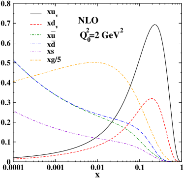
Figure 1: (Color online) Parton distribution for free proton at $Q_{0}^{2}=2$  GeV².

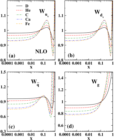
Figure 2: (Color online) Weight function for Fe, Ca, C, He and D nuclei, sub-leveled by (a) to (d) for different types of PDFs .

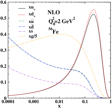
Figure 3: (Color online) Parton distribution for ${}^{56}Fe$ at $Q_{0}^{2}=2$  GeV².

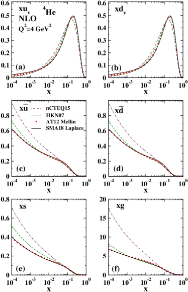
Figure 4: (Color online) Parton distribution function for ⁴He at $Q^{2}=4$ GeV², resulted from the Laplace transform, represented by the solid line (SMA18 Laplace) which has been compared with the AT12 AtashbarTehrani:2012xh , HKN07 Hirai:2007sx and nCTEQ15 Kovarik:2015cma models. The plots for different types of PDFs are specified by sub-level (a) to (f).

Figure 5: (Color online) Parton distribution function for ⁵⁶Fe at $Q^{2}=4$  GeV² , resulted from the Laplace transform, represented by the solid line (SMA18 Laplace) which has been compared with the AT12 AtashbarTehrani:2012xh , HKN07 Hirai:2007sx and nCTEQ15 Kovarik:2015cma models. The plots for different types of PDFs are specified by sub-level (a) to (f).

Now if we intend to get the solution for the nonsinglet part, $F_{\rm NS}(x,Q^{2})$, its NLO contribution can be written as :

$$\frac{4\pi}{\alpha_{s}(Q^{2})} \frac{\partial F_{\rm NS}}{\partial lnQ^{2}}(x,Q^{2})$$

$$=F_{NS}\otimes\left(p_{qq}^{\rm LO,NS}+\frac{\alpha_{s}(Q^{2})}{4\pi}p_{qq}^{\rm NLO,NS}\right)(x,Q^{2})\,.$$

The first order differential equations in Laplace $s$-space for the non-singlet distribution and in terms of the $\tau$ variable, can be obtained as in  Block:2010du ; Khanpour:2016uxh ; Block:2011xb :

$f_{\rm NS}(s,\tau)$,

$$\frac{\partial f_{\rm NS}}{\partial\tau}(s,\tau)=\left(\Phi_{\rm NS}^{\rm LO}+\frac{\alpha_{s}(\tau)}{4\pi}\Phi_{\rm NS,qq}^{\rm NLO}\right)f_{\rm NS}(s,\tau)\,.$$ (13)

The solution of the above equation would simply be

$$f_{\rm NS}(s,\tau)=e^{\tau\Phi_{\rm NS}(s)}f^{0}_{\rm NS}(s)\;.$$ (14)

Here $\Phi_{\rm NS}(s)$ includes the NLO contribution of the splitting functions in $s$ space such that

$$\Phi_{\rm NS}(s)\equiv\Phi_{\rm NS}^{\rm LO}(s)+\frac{\tau_{2}}{\tau}\Phi_{\rm NS,qq}^{\rm NLO}(s)\,.$$ (15)

Evaluation of $\Phi_{\rm NS,qq}^{\rm NLO}(s)={\cal L}\left[e^{-\nu}p_{qq}^{\rm NLO,NS}(e^{-\nu});s\right]$ is too lengthy but straightforward and its analytical result in the transformed Laplace $s$ space at NLO approximation is given in Appendix A of Ref. Khanpour:2016uxh .

To amend the notations which are used in the article, it should be noted that at the leading order approximation, $Q^{2}$ dependence of the evolution equation is in fact represented by $\tau$ variable and at the NLO approximation, by $\tau_{2}$; the former is defined in Refs. Block:2010du ; Khanpour:2016uxh ; Block:2011xb ; AtashbarTehrani:2013qea ,

$$\tau_{2}\equiv\frac{1}{4\pi}\int_{0}^{\tau}\alpha(\tau^{\prime})d\tau^{\prime}\ =\ (\frac{1}{4\pi})^{2}\int_{Q_{0}^{2}}^{Q^{2}}\alpha_{s}^{2}(Q^{\prime 2})\ d\ln Q^{\prime 2}\,.$$

We should use the variable $\tau_{2}$ since the current analysis is done at NLO approximation but for simplicity in the notation, $\tau$ will be used in the remainder of the paper in its place. It should be finally noted that the NLO expansion parameter, $a_{1}$, in the iterative solution of Eq.(9) is quite small. For instance $a_{1}=0.025$ for $M^{2}_{c}<Q^{2}\leq M^{2}_{b}GeV^{2}$ while $b_{1}=10.7$ and $a_{1}=0.017$ with $b_{1}=8.63$ for $M^{2}_{b}<Q^{2}\leq 10^{5}GeV^{2}$. Furthermore, $a_{0}=0.025$ and is constant over the whole range of $Q^{2}$ scale  [II].

III Theoretical formalism for the EMC effect

To calculate the parton distribution in nuclear media, we would need to have the parton distributions for a free proton. To achieve this, it is required to use a set of PDFs at the input scale $Q_{0}^{2}=2\;GeV^{2}$ which are depicting in Fig. 1 and have the following standard parametrization, as in Ref. Khanpour:2012tk :

$$xu_{v} = 0.37328x^{0.32182}(1-x)^{3.59165}$$

$$(1+3.62456x^{0.50629}+21.31705x),$$

$$xd_{v} = 0.51354x^{0.39354}(1-x)^{5.03622}$$

$$(1-1.26057x^{0.47037}+15.98368x),$$

$$2x(\overline{d}+\overline{u}) = 0.29795x^{-0.2052}(1-x)^{9.06901}$$

$$(1+0.93542x^{0.33012}+14.46062x),$$

$$x(\overline{d}-\overline{u}) = 9.49265x^{1.33727}(1-x)^{18.559}$$

$$(1-7.82741x^{0.54431}+20.60532x),$$

$$xs = 0.03724x^{-0.2052}(1-x)^{9.06901}$$

$$(1+0.93542x^{0.33012}+14.46062x),$$

$$xg = 3.60703x^{0.062467}(1-x)^{6.75001}$$ (17)

$$(1+3.91106x^{2}-0.813601x).$$

On the other hand, using a number of parameters, the nPDFs are specified at a fixed $Q^{2}$ which is usually taken as $Q_{0}^{2}$. There is a relation between the nPDFs and the PDFs in free proton in which the PDFs are multiplied by a weight function $w_{i}$ such that Hirai:2001np :

$$f_{i}^{A}(x,Q_{0}^{2})=w_{i}(x,A,Z)f_{i}(x,Q_{0}^{2})$$ (18)

Using a $\chi^{2}$ analysis procedure, the parameters in the weight function which are dependent on $x$, $A$ (atomic mass), and $Z$ (atomic number), can be obtained.

The following functional forms would be assumed for the weight function in Eq. (18) which are based on the analysis in Refs. Hirai:2001np ; Hirai:2004wq ; Hirai:2007sx ; Tehrani:2004hp ; Tehrani:2006gy ; Tehrani:2007hu ; AtashbarTehrani:2012xh ; Khanpour:2016pph :

$$w_{i} = 1+\left(1-\frac{1}{A^{\alpha_{i}}}\right)$$ (19)

$$\times\frac{a_{i}(A,Z)+b_{i}(A)x+c_{i}(A)x^{2}+d_{i}(A)x^{3}}{(1-x)^{\beta_{i}}}$$

The following nPDFs can be obtained, considering the weight function in Eq. (19) which is combined with PDFs in Eq. (III):

$$u_{v}^{A}(x,Q_{0}^{2}) = w_{u_{v}}(x,A,Z)\frac{Zu_{v}(x,Q_{0}^{2})+Nd_{v}(x,Q_{0}^{2})}{A},$$

$$d_{v}^{A}(x,Q_{0}^{2}) = w_{d_{v}}(x,A,Z)\frac{Zd_{v}(x,Q_{0}^{2})+Nu_{v}(x,Q_{0}^{2})}{A},$$

$$\overline{u}^{A}(x,Q_{0}^{2}) = w_{\overline{q}}(x,A,Z)\frac{Z\overline{u}(x,Q_{0}^{2})+N\overline{d}(x,Q_{0}^{2})}{A},$$

$$\overline{d}^{A}(x,Q_{0}^{2}) = w_{\overline{q}}(x,A,Z)\frac{Z\overline{d}(x,Q_{0}^{2})+N\overline{u}(x,Q_{0}^{2})}{A},$$

$$s^{A}(x,Q_{0}^{2}) = w_{\overline{q}}(x,A,Z)s(x,Q_{0}^{2}),$$

$$g^{A}(x,Q_{0}^{2}) = w_{g}(x,A,Z)g(x,Q_{0}^{2}).$$ (20)

The $Z$ term and the $N(=A-Z)$ term in the above equations are indicating the atomic number (the number of protons) and the number of neutrons in the nuclei respectively. Here the SU(3) symmetry is not assumed.

For the case of isoscalar nuclei in which the number of protons and neutrons in a nucleus are equal to each other, valence quarks as well as anti-quark would have similar distributions. But since in heavy nuclei the number of the neutrons is larger than the number of protons $(N>Z)$, as can be seen in Eq.(20), the distribution of down valence quarks would be greater than that of up valence quarks. Following that, it can be seen, as well, that in this type of the nuclei, antiquark distributions $(\overline{u}^{A},\overline{d}^{A},\overline{s}^{A})$ would not be equal to each other  Kumano:1997cy ; Garvey:2001yq .

As in Ref. Sick:1992pw , $\alpha_{i}$ is taken to have the value $1/3$ in Eq. (19). Also it should be noted that, there exist three constraints on the parameters in the equation, considering nuclear volume and surface contributions. These constraints are related to the nuclear charge $Z$, baryon number ( atomic number) $A$ and momentum conservation  Hirai:2001np ; Hirai:2004wq ; AtashbarTehrani:2012xh ; Frankfurt:1990xz , which can be written in the Laplace space as follows:

$$Z = \frac{A}{3}{\cal L}[2e^{-v}u_{v}^{A}(e^{-v},Q_{0}^{2})-e^{-v}d_{v}^{A}(e^{-v},Q_{0}^{2});s=0],$$

$$A = \frac{A}{3}{\cal L}[e^{-v}u_{v}^{A}(e^{-v},Q_{0}^{2})+e^{-v}d_{v}^{A}(e^{-v},Q_{0}^{2});s=0],$$

$$A = A{\cal L}\{e^{-v}[u_{v}^{A}+d_{v}^{A}+2(\overline{u}^{A}+\overline{d}^{A}+s^{A})+g^{A}](e^{-v},Q_{0}^{2});s=1\}.$$

In order to be able to do the required calculations for iron (Fe), calcium (Ca), carbon (C), helium (He) and deuterium (D) nuclei, we need the relevant weight functions which are presented in the following relations in which the effects of shadowing, anti-shadowing, fermi motion and the EMC regions are included  AtashbarTehrani:2012xh :

$$w_{u_{v}}^{Fe} = 1+\left(1-\frac{1}{56^{1/3}}\right)\frac{-0.0979153+2.08684x-6.91749x^{2}+5.50217x^{3}}{(1-x)^{0.4}}$$

$$w_{d_{v}}^{Fe} = 1+\left(1-\frac{1}{56^{1/3}}\right)\frac{-0.0980722+2.08684x-6.91749x^{2}+5.50217x^{3}}{(1-x)^{0.4}}$$

$$w_{\overline{q}}^{Fe} = 1+\left(1-\frac{1}{56^{1/3}}\right)\frac{-0.344557+7.71619x-45.8738x^{2}+66.9498x^{3}}{(1-x)^{0.1}}$$

$$w_{g}^{Fe} = 1+\left(1-\frac{1}{56^{1/3}}\right)\frac{-0.305125+2.59586x+0.369233x^{3}}{(1-x)^{0.1}}$$ (22)

$$w_{u_{v}}^{Ca} = 1+\left(1-\frac{1}{40^{1/3}}\right)\frac{-0.0972234+2.08106x-6.90323x^{2}+5.47457x^{3}}{(1-x)^{0.4}}$$

$$w_{d_{v}}^{Ca} = 1+\left(1-\frac{1}{40^{1/3}}\right)\frac{-0.0972234+2.08106x-6.90323x^{2}+5.47457x^{3}}{(1-x)^{0.4}}$$

$$w_{\overline{q}}^{Ca} = 1+\left(1-\frac{1}{40^{1/3}}\right)\frac{-0.325852+7.19981x-42.7529x^{2}+60.2908x^{3}}{(1-x)^{0.1}}$$

$$w_{g}^{Ca} = 1+\left(1-\frac{1}{40^{1/3}}\right)\frac{-0.300195+2.59586x+0.369233x^{3}}{(1-x)^{0.1}}$$ (23)

$$w_{u_{v}}^{C} = 1+\left(1-\frac{1}{12^{1/3}}\right)\frac{-0.0944919+2.0605x-6.85243x^{2}+5.37693x^{3}}{(1-x)^{0.4}}$$

$$w_{d_{v}}^{C} = 1+\left(1-\frac{1}{12^{1/3}}\right)\frac{-0.0944919+2.0605x-6.85243x^{2}+5.37693x^{3}}{(1-x)^{0.4}}$$

$$w_{\overline{q}}^{C} = 1+\left(1-\frac{1}{12^{1/3}}\right)\frac{-0.266859+5.61929x-33.2257x^{2}+41.4429x^{3}}{(1-x)^{0.1}}$$

$$w_{g}^{C} = 1+\left(1-\frac{1}{12^{1/3}}\right)\frac{-0.288775+2.59586x+0.369233x^{3}}{(1-x)^{0.1}}$$ (24)

$$w_{u_{v}}^{He} = 1+\left(1-\frac{1}{4^{1/3}}\right)\frac{-0.0920426+2.04191x-6.8064x^{2}+5.28935x^{3}}{(1-x)^{0.4}}$$

$$w_{d_{v}}^{He} = 1+\left(1-\frac{1}{4^{1/3}}\right)\frac{-0.0920426+2.04191x-6.8064x^{2}+5.28935x^{3}}{(1-x)^{0.4}}$$

$$w_{\overline{q}}^{He} = 1+\left(1-\frac{1}{4^{1/3}}\right)\frac{-0.2224+4.48189x-26.3976x^{2}+29.4371x^{3}}{(1-x)^{0.1}}$$

$$w_{g}^{He} = 1+\left(1-\frac{1}{4^{1/3}}\right)\frac{-0.284205+2.59586x+0.369233x^{3}}{(1-x)^{0.1}}\allowdisplaybreaks[1]$$ (25)

$$w_{u_{v}}^{D} = 1+\left(1-\frac{1}{2^{1/3}}\right)\frac{-0.0905182+2.03027x-6.77752x^{2}+5.23484x^{3}}{(1-x)^{0.4}}$$

$$w_{d_{v}}^{D} = 1+\left(1-\frac{1}{2^{1/3}}\right)\frac{-0.0905182+2.03027x-6.77752x^{2}+5.23484x^{3}}{(1-x)^{0.4}}$$

$$w_{\overline{q}}^{D} = 1+\left(1-\frac{1}{2^{1/3}}\right)\frac{-0.198243+3.8859x-22.8312x^{2}+23.7229x^{3}}{(1-x)^{0.1}}$$

$$w_{g}^{D} = 1+\left(1-\frac{1}{2^{1/3}}\right)\frac{-0.283108+2.59586x+0.369233x^{3}}{(1-x)^{0.1}}$$ (26)

In Fig. 2, the weight functions for the Fe, Ca, C, He, and D nuclei are depicting at the initial scale $Q_{0}^{2}=2$  GeV² and in Fig. 3, the parton distribution functions inside ${}^{56}Fe$ nucleus at $Q_{0}^{2}=2$ GeV² are presented.

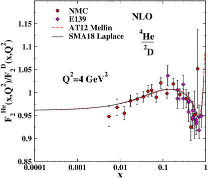
Figure 6: (Color online) EMC effect for ⁴He/²D at $Q^{2}=4$ GeV², resulted from the Laplace transform , represented by solid line (SMA18 Laplace) which has been compared with the AT12 model  AtashbarTehrani:2012xh and DIS data of NMC Amaudruz:1995tq and E139 Gomez:1993ri Collaborations.

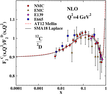
Figure 7: (Color online) EMC effect for ¹²C/²D at $Q^{2}=4$ GeV², resulted from the Laplace transform, , represented by solid line (SMA18 Laplace) which has been compared with the AT12 model AtashbarTehrani:2012xh and DIS data of NMC Arneodo:1995cs , EMC Ashman:1988bf , E139 Gomez:1993ri and E665 Adams:1995is Collaborations.

Figure 8: (Color online) EMC effect for ⁴⁰Ca/²D at $Q^{2}=4$ GeV² resulted from the Laplace transform, represented by solid line (SMA18 Laplace) which has been compared with the AT12 model AtashbarTehrani:2012xh and DIS data of NMC Arneodo:1995cs , EMC Ashman:1988bf , E139 Gomez:1993ri and E665 Adams:1995is Collaborations.

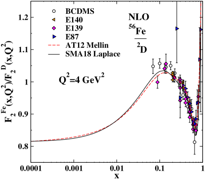
Figure 9: (Color online) EMC effect for ⁵⁶Fe/²D at $Q^{2}=4$ GeV² resulted from the Laplace transform, represented by a solid line (SMA18 Laplace) which has been compared with the AT12 model AtashbarTehrani:2012xh and DIS data of BCDMS Benvenuti:1987az , E140 Dasu:1988ru , E139 Gomez:1993ri and finally E87 Bodek:1983qn Collaborations.

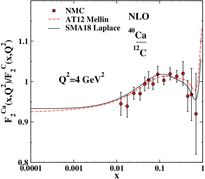
Figure 10: (Color online) EMC effect for ${}^{40}Ca/^{12}C$ at $Q^{2}=4\;GeV^{2}$ resulted from the Laplace transform, represented by solid line (SMA18 Laplace) which has been compared with the AT12 model AtashbarTehrani:2012xh and DIS data in nuclear reaction NMC Amaudruz:1995tq .

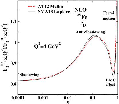
Figure 11: (Color online) EMC effect for ⁵⁶Fe/²D at $Q^{2}=4$ GeV² resulted from the Laplace transform, represented by a solid line (SMA18 Laplace) which has been compared with the AT12 model AtashbarTehrani:2012xh while the anti-shadowing, shadowing, EMC and fermi motion regions are included.

IV Nuclear structure function $F_{2}^{A}(x,Q^{2})$ in the Laplace space

Based on the Laplace transform technique, we perform here an analytical calculation of the nuclear structure function $F_{2}^{A}(x,Q^{2})$ at NLO approximation. We should first extract the nucleon structure function, using the singlet, gluon and non-singlet parton distributions which were obtained in the previous sections. The nuclear structure function $F_{2}^{A}(x,Q^{2})$ in Laplace $s$ space, up to the next-to-leading order approximation, can be written as

$${\cal F}_{2}^{\rm A}(s,\tau)={\cal F}_{2}^{\rm S}(s,\tau)+{\cal F}_{2}^{G}(s,\tau)+{\cal F}_{2}^{\rm NS}(s,\tau)\,,$$ (27)

where the flavour singlet ${\cal F}_{2}^{\rm S}$ and gluon ${\cal F}_{2}^{G}$ contribution reads

$${\cal F}_{2}^{\rm S}(s,\tau) = \left(\frac{4}{9}2\bar{u}^{A}(s,\tau)+\frac{1}{9}2\bar{d}^{A}(s,\tau)+\frac{1}{9}2\bar{s}^{A}(s,\tau)\right)$$ (28)

$$\times\left(1+\frac{\tau}{4\pi}C^{(1)}_{q}(s)\right)\,,$$

$${\cal F}_{2}^{\rm G}(s,\tau) = \frac{2}{9}g^{A}(s,\tau)\left(\frac{\tau}{4\pi}C^{(1)}_{g}(s)\right)\,.$$ (29)

Finally, the non-singlet contribution for three active (light) flavours is given by

$${\cal F}_{2}^{\rm NS}(s,\tau) = \left(\frac{4}{9}u_{v}^{A}(s,\tau)+\frac{1}{9}d_{v}^{A}(s,\tau)\right)\left(1+\frac{\tau}{4\pi}C^{(1)}_{q}(s)\right)\;,$$

where $C_{q}^{(1)}(s)$ and $C_{g}^{(1)}(s)$ represent Wilson coefficients functions at NLO and can be derived in Laplace $s$ space by $c_{q}(s)={\cal L}[e^{-\nu}c_{q}(e^{-\nu});s]$ and $c_{g}(s)={\cal L}[e^{-\nu}c_{g}(e^{-\nu});s]$. Explicit expressions for the corresponding Wilson coefficients functions are as follow Khanpour:2016uxh :

$$C_{q}^{(1)}(s)=$$

$$C_{F}\left(-9-\frac{2\pi^{2}}{3}-\frac{2}{(1+s)^{2}}+\frac{6}{1+s}-\frac{2}{(2+s)^{2}}+\frac{4}{2+s}+\right.$$

$$3\left(\gamma_{E}+\psi(s+1)\right)+\frac{2\left(\gamma_{E}+\psi(s+2)\right)}{1+s}+\frac{2\left(\gamma_{E}+\psi(s+3)\right)}{2+s}+$$

$$\left.\frac{1}{3}\left(\pi^{2}+6\left(\gamma_{E}+\psi(s+1)\right){}^{2}-6\psi^{\prime}(s+1)\right)+4\psi^{\prime}(s+1)\right)\,,$$

$$C_{g}^{(1)}(s)=$$

$$f\left(\frac{2}{(1+s)^{2}}-\frac{2}{1+s}-\frac{4}{(2+s)^{2}}+\frac{16}{2+s}+\frac{4}{(3+s)^{2}}-\frac{16}{3+s}-\right.$$

$$\left.\frac{2\left(\gamma_{E}+\psi(s+2)\right)}{1+s}+\frac{4\left(\gamma_{E}+\psi(s+3)\right)}{2+s}-\frac{4\left(\gamma_{E}+\psi(s+4)\right)}{3+s}\right)\,.$$

As before, $Q^{2}$ dependence of the nuclear structure function in Eq. (27) is given again by $\tau(Q^{2},Q_{0}^{2})\equiv{1\over 4\pi}\int_{Q^{2}_{0}}^{Q^{2}}\alpha_{s}({Q^{\prime}}^{2})d\,\ln{Q^{\prime}}^{2}$. Using the inverse Laplace transform and the appropriate change of variables Khanpour:2016uxh , the desired solution for the nuclear structure function in Bjorken $x$ space, $F_{2}^{\rm A}(x,Q^{2})$, can be readily obtained.

V Laplace transformation technique and the EMC results

Based on the analytical solution for the DGLAP evolution equations, using the Laplace transformation technique, we shall first present in this section our results that have been obtained for the parton distribution functions after which the nuclear structure function ratio $F_{2}^{A^{\prime}}(x,Q^{2})/F_{2}^{A}(x,Q^{2})$ would be presented. Figure  2 illustrates the weight function for ⁵⁶Fe, ⁴⁰Ca, ¹²C, ⁴He and ²D nuclei. In Fig. 3, we depict parton distribution functions inside ${}^{56}Fe$ nucleus at $Q_{0}^{2}=2$ GeV² while according to Eq. (20) SU(3) symmetry breaking is supposed to be in place and hence the down anti-quark distribution is assumed to be larger than the up anti-quark distribution where additionally we see as well that down valence quark distribution is greater than up valence distribution. Based on Eq. (14), the required calculations could be performed to obtain, at the NLO approximation, the valence quark distributions, $xu_{v}^{A}(x,Q^{2})$ and $xd_{v}^{A}(x,Q^{2})$. In Figs. 4,and 5, these distributions have been presented alongside other parton distributions, including the anti-quarks and gluon distribution functions for ⁴He and ⁵⁶Fe nuclei at $Q^{2}=4$ GeV² in Laplace $s$-space. Furthermore, they have been compared with AT12 AtashbarTehrani:2012xh , HKN07 Hirai:2007sx and nCTEQ15  Kovarik:2015cma models. As can be seen, a good agreement does exist between the presented results and the results obtained from the other models. The solid line represents our solution, resulting from the Laplace transform technique and the red circles represent the parton quark distributions from the AT12 model.

In Fig. 6, the EMC effect has been demonstrated for ⁴He nucleus in Laplace s space and Mellin space AtashbarTehrani:2012xh at $Q^{2}=4$  GeV² and compared with DIS data in nuclear reactions from NMC Amaudruz:1995tq and E139 Gomez:1993ri Collaborations. The EMC effect for ${}^{12}C$ nucleus in Laplace s-space and Mellin momment space  AtashbarTehrani:2012xh at $Q^{2}=4$ GeV² has been shown in Fig. 7 and they have been compared with the results from the DIS data in nuclear reactions NMC Arneodo:1995cs as well as EMC Ashman:1988bf , E139 Gomez:1993ri and E665 Adams:1995is collaborations. The corresponding results for the EMC effect in ⁴⁰Ca structure function in Laplace $s$- space and Mellin moment space AtashbarTehrani:2012xh at $Q^{2}=4$  GeV² have been presented inn Fig. 8 and compared with the results from DIS data in nuclear reactions by NMC Amaudruz:1995tq and EMC Arneodo:1989sy , E139  Gomez:1993ri , and E665 Adams:1995is Collaborations.

It is seen that our analytical solutions based on the inverse Laplace transform technique at the NLO approximation for the nuclear structure function over a wide range of $x$ and $Q^{2}$ values, correspond well with the experimental data and the AT12 model. One can conclude that, in spite of small disagreements for the parton densities, we find a satisfactory agreement for the nuclear structure function ratio over a wide range of $x$’s and $Q^{2}$’s. The overall agreement is found to have a deviation of 1 part in 10⁵. In Fig. 9, we present the EMC effect for ⁵⁶Fe structure function in Laplace space and Mellin space AtashbarTehrani:2012xh at $Q^{2}=4$ GeV² and a comparison with the DIS data in nuclear reactions BCDMS Benvenuti:1987az , and also E140 Dasu:1988ru , E139  Gomez:1993ri , and E87 Bodek:1983qn Collaborations is done.

Finally, in Fig. 10 we compare the EMC effect for ⁴⁰Ca/¹²C structure function in Laplace $s$-space as well as in the Mellin moment space  AtashbarTehrani:2012xh at $Q^{2}=4$  GeV² with the DIS data from the NMC Collaboration Amaudruz:1995tq . In all figures, including for example Fig. 11, the effects of the shadowing region and Fermi region are identical in the Mellin and Laplace spaces while the effect of the anti-shawdowing region and EMC region in Laplace space are more acceptable and better than in the Mellin space.

VI Summary and conclusion

The result for NLO decoupled analytical evolution equations for singlet $F_{\rm S}(x,Q^{2})$, gluon $G(x,Q^{2})$ and non-singlet $F_{\rm NS}(x,Q^{2})$ have been presented in this article, which resulted from the solution of coupled DGLAP evolution equations in the Laplace $s$-space. Following that, we performed the required calculations and obtained the results for valence quark distributions $xu_{v}$ and $xd_{v}$, the anti-quark distributions $x\overline{d}$ and $x\overline{u}$, the strange sea distribution $xs=x\overline{s}$ and finally the gluon distribution $xg$, using the input parton distributions at $Q_{0}^{2}$ = 2  GeV² for free protons which is initiated from the KKT12 model  Khanpour:2012tk . We also calculated in this work, the nuclear structure function $F_{2}^{A}(x,Q^{2})$ which is a direct result from the Laplace transform technique. To derive this structure function, the corresponding analytical solutions for singlet $F_{2}^{\rm S}(x,Q^{2})$, gluon $F_{2}^{\rm G}(x,Q^{2})$ and non-singlet $F_{2}^{\rm NS}(x,Q^{2})$ structure functions, inside the nucleus, are needed. Having the initial distributions for singlet, gluon and non-singlet distributions at the input scale $Q_{0}^{2}$, we could obtain the nuclear structure function at any arbitrary $Q^{2}$ scale. The employed method, in our analysis, creates the possibility of obtaining a strictly analytical solution in terms of the $x$-variable for nuclear parton densities as well as the structure function . As a final point, we got the general solutions such that they are in satisfactory agreement with AT12, HKN07, and nCTEQ15 models and also with the available experimental data including those of the NMC, BCDMS, E87, E139, E140, and E65 Collaborations. As a further research task, it is possible to extend the calculation up to NNLO approximation to investigate the EMC effect, using the Laplace transformation while new updated data are employed. We hope to report on this issue in future.

References

• (1) J. C. Collins, D. E. Soper and G. F. Sterman, “Factorization for Short Distance Hadron - Hadron Scattering,” Nucl. Phys. B 261, 104 (1985).
• (2) G. T. Bodwin, “Factorization of the Drell-Yan Cross-Section in Perturbation Theory,” Phys. Rev. D 31, 2616 (1985). Erratum: Phys. Rev. D 34, 3932 (1986).
• (3) J. C. Collins, “Hard scattering factorization with heavy quarks: A General treatment,” Phys. Rev. D 58, 094002 (1998).
• (4) P. Hoodbhoy and R. L. Jaffe, “Quark Exchange in Nuclei and the Emc Effect,” Phys. Rev. D 35, 113 (1987).
• (5) Arifuzzaman, S. H. Hasan and P. Hoodbhoy, “Quark Exchange Contribution to the European Muon Collaboration Effect in Nuclear Matter,” Phys. Rev. C 38, 498 (1988).
• (6) Y. L. Dokshitzer, “Calculation of the Structure Functions for Deep Inelastic Scattering and $e^{+}e^{-}$ Annihilation by Perturbation Theory in Quantum Chromodynamics.,” Sov. Phys. JETP 46, 641 (1977) [Zh. Eksp. Teor. Fiz.  73, 1216 (1977)].
• (7) V. N. Gribov and L. N. Lipatov, “Deep inelastic e p scattering in perturbation theory,” Sov. J. Nucl. Phys.  15, 438 (1972) [Yad. Fiz.  15, 781 (1972)].
• (8) L. N. Lipatov, “The parton model and perturbation theory,” Sov. J. Nucl. Phys.  20, 94 (1975) [Yad. Fiz.  20, 181 (1974)].
• (9) G. Altarelli and G. Parisi, “Asymptotic Freedom in Parton Language,” Nucl. Phys. B 126, 298 (1977).
• (10) M. M. Block, L. Durand, P. Ha and D. W. McKay, “Decoupling the NLO coupled DGLAP evolution equations: an analytic solution to pQCD,” Eur. Phys. J. C 69, 425 (2010).
• (11) M. M. Block, L. Durand, P. Ha and D. W. McKay, “Applications of the leading-order Dokshitzer-Gribov-Lipatov-Altarelli-Parisi evolution equations to the combined HERA data on deep inelastic scattering,” Phys. Rev. D 84, 094010 (2011).
• (12) M. M. Block, L. Durand, P. Ha and D. W. McKay, “An Analytic solution to LO coupled DGLAP evolution equations: a new pQCD tool,” Phys. Rev. D 83, 054009 (2011).
• (13) M. M. Block, “A New numerical method for obtaining gluon distribution functions $G(x,Q^{2})=xg(x,Q^{2})$, from the proton structure function $F_{2}^{\gamma p}(x,Q^{2})$,” Eur. Phys. J. C 65, 1 (2010).
• (14) M. M. Block, “Addendum to: ‘A new numerical method for obtaining gluon distribution functions $G(x,Q^{2})=xg(x,Q^{2})$, from the proton structure function $F_{2}^{\gamma p}(x,Q^{2})$.’,” Eur. Phys. J. C 68, 683 (2010).
• (15) G. R. Boroun, S. Zarrin and F. Teimoury, “Decoupling of the DGLAP evolution equations by Laplace method,” Eur. Phys. J. Plus 130, 214 (2015).
• (16) G. R. Boroun and B. Rezaei, “Decoupling of the DGLAP evolution equations at next-to-next-to-leading order (NNLO) at low-x,” Eur. Phys. J. C 73, 2412 (2013).
• (17) M. Zarei, F. Taghavi-Shahri, S. Atashbar Tehrani and M. Sarbishei, “Fragmentation functions of the pion, kaon, and proton in the NLO approximation: Laplace transform approach,” Phys. Rev. D 92, 074046 (2015).
• (18) F. Taghavi-Shahri, S. Atashbar Tehrani and M. Zarei, “Fragmentation functions of neutral mesons $\pi^{0}$ and $k^{0}$ with Laplace transform approach,” Int. J. Mod. Phys. A 31, 1650100 (2016).
• (19) H. Khanpour, A. Mirjalili and S. Atashbar Tehrani, “Analytic derivation of the next-to-leading order proton structure function $F_{2}^{p}(x,Q^{2})$ based on the Laplace transformation,” Phys. Rev. C 95, 035201 (2017).
• (20) S. M. Moosavi Nejad, H. Khanpour, S. Atashbar Tehrani and M. Mahdavi, “QCD analysis of nucleon structure functions in deep-inelastic neutrino-nucleon scattering: Laplace transform and Jacobi polynomials approach,” Phys. Rev. C 94, 045201 (2016).
• (21) S. Atashbar Tehrani, F. Taghavi-Shahri, A. Mirjalili and M. M. Yazdanpanah, “NLO analytical solutions to the polarized parton distributions, based on the Laplace transformation,” Phys. Rev. D 87, 114012 (2013)
Erra:Phys. Rev. D 88, 039902 (2013).
• (22) M. Salajegheh, S. M. Moosavi Nejad, M. Nejad, H. Khanpour and S. Atashbar Tehrani, “Analytical approaches to the determination of spin-dependent parton distribution functions at NNLO approximation,” Phys. Rev. C 97, 055201 (2018).
• (23) S. Atashbar Tehrani, “Nuclear parton densities and their uncertainties at the next-to-leading order,” Phys. Rev. C 86, 064301 (2012).
• (24) M. M. Block, L. Durand and D. W. McKay, “Analytic derivation of the leading-order gluon distribution function $G(x,Q^{2})=xg(x,Q^{2})$ from the proton structure function $F_{2}^{p}(x,Q^{2})$,” Phys. Rev. D 77, 094003 (2008).
• (25) M. M. Block, L. Durand and D. W. McKay, “Analytic treatment of leading-order parton evolution equations: Theory and tests,” Phys. Rev. D 79, 014031 (2009).
• (26) G. Curci, W. Furmanski and R. Petronzio, “Evolution of Parton Densities Beyond Leading Order: The Nonsinglet Case,” Nucl. Phys. B 175, 27 (1980).
• (27) W. Furmanski and R. Petronzio, “Singlet Parton Densities Beyond Leading Order,” Phys. Lett. B 97, 437 (1980).
• (28) M. Botje, “QCDNUM: Fast QCD Evolution and Convolution,” Comput. Phys. Commun. 182, 490 (2011).
• (29) E. G. Floratos, C. Kounnas and R. Lacaze, “Higher Order QCD Effects in Inclusive Annihilation and Deep Inelastic Scattering,” Nucl. Phys. B 192, 417 (1981).
• (30) H. Khanpour, A. N. Khorramian and S. Atashbar Tehrani, “New parton distributions in fixed flavour factorization scheme from recent deep-inelastic-scattering data,” J. Phys. G 40, 045002 (2013).
• (31) M. Hirai, S. Kumano and M. Miyama, “Determination of nuclear parton distributions,” Phys. Rev. D 64, 034003 (2001).
• (32) M. Hirai, S. Kumano and T.-H. Nagai, “Nuclear parton distribution functions and their uncertainties,” Phys. Rev. C 70, 044905 (2004).
• (33) M. Hirai, S. Kumano and T.-H. Nagai, “Determination of nuclear parton distribution functions and their uncertainties in next-to-leading order,” Phys. Rev. C 76, 065207 (2007).
• (34) S. Atashbar Tehrani, A. N. Khorramian and A. Mirjalili, “Nuclear parton densities and structure functions,” Int. J. Mod. Phys. A 20, 1927 (2005).
• (35) S. Atashbar Tehrani, A. Mirjalili and A. N. Khorramian, “EMC effect and nuclear structure functions,” Nucl. Phys. Proc. Suppl. 164, 30 (2007).
• (36) S. Atashbar Tehrani and A. N. Khorramian,"QCD Analysis for Nuclear Parton Distributions in the Next to Leading Order" in MENU 2007: 11th International Conference on Meson-Nucleon Physics and the Structure of the Nucleon, IKP, Forschungzentrum Jülich, Germany, 2007, edited by H.Machner and S. Krewald, SLAC eConf C070910 (SLAC, Stanford, 2007).
• (37) H. Khanpour and S. Atashbar Tehrani, “Global Analysis of Nuclear Parton Distribution Functions and Their Uncertainties at Next-to-Next-to-Leading Order,” Phys. Rev. D 93, 014026 (2016).
• (38) S. Kumano, “Flavor asymmetry of anti-quark distributions in the nucleon,” Phys. Rept. 303, 183 (1998).
• (39) G. T. Garvey and J. C. Peng, “Flavor asymmetry of light quarks in the nucleon sea,” Prog. Part. Nucl. Phys. 47, 203 (2001).
• (40) I. Sick and D. Day, “The EMC effect of nuclear matter,” Phys. Lett. B 274, 16 (1992).
• (41) L. L. Frankfurt, M. I. Strikman and S. Liuti, “Evidence for enhancement of gluon and valence quark distributions in nuclei from hard lepton nucleus processes,” Phys. Rev. Lett. 65, 1725 (1990).
• (42) K. Kovarik et al., “nCTEQ15 - Global analysis of nuclear parton distributions with uncertainties in the CTEQ framework,” Phys. Rev. D 93, 085037 (2016).
• (43) P.Amaudruz, M.Arneodom, A.Arvidson, B.Badelek, M.Ballintijn, G.Baum, J.Beaufays, I.G.Bird, P.Björkholm, M.Botje, et al. [New Muon Collaboration], “A Reevaluation of the nuclear structure function ratios for D, He, Li-6, C and Ca,” Nucl. Phys. B 441, 3 (1995).
• (44) J. Gomez, R. G. Arnold, P. E. Bosted, C. C. Chang, A. T. Katramatou, G. G. Petratos, A. A. Rahbar, S. E. Rock, A. F. Sill, Z. M. Szalata,et al., “Measurement of the A-dependence of deep inelastic electron scattering,” Phys. Rev. D 49, 4348 (1994).
• (45) M.Arneodo, A.Arvidson, B.Badełek, M.Ballintijn, G.Baum, J.Beaufays, I.G.Bird, P.Björkholm, M.Botje, C.Broggini et al. [New Muon Collaboration], “The Structure Function ratios $F_{2}(li)/F_{2}(D)$ and $F_{2}(C)/F_{2}(D)$ at small x,” Nucl. Phys. B 441, 12 (1995).
• (46) J.Ashman, B.Badelek, G.Baum, J.Beaufays, C.P.Bee, C.Benchouk, I.G.Bird, S.C.Brown, M.C.Caputo, H.W.K.Cheung, et al. [European Muon Collaboration], “Measurement of the Ratios of Deep Inelastic Muon - Nucleus Cross-Sections on Various Nuclei Compared to Deuterium,” Phys. Lett. B 202, 603 (1988).
• (47) M. R. Adams, S. Aïd, P. L. Anthony, D. A. Averill, M. D. Baker, B. R. Baller, A. Banerjee, A. A. Bhatti, U. Bratzler, H. M. Braun et al. [E665 Collaboration], “Shadowing in inelastic scattering of muons on carbon, calcium and lead at low x(Bj),” Z. Phys. C 67, 403 (1995).
• (48) M.Arneodo, A.Arvidson, J.J.Aubert, B.Badelek, J.Beaufays, C.P.Bee, C.Benchouk, G.Berghoff, I.G.Bird, D.Blum et al. [European Muon Collaboration], “Measurements of the nucleon structure function in the range $0.002-{\rm GeV}^{2}<x<0.17-{\rm GeV}^{2}$ and $0.2-GeV^{2}<Q^{2}<8-GeV^{2}$ in deuterium, carbon and calcium,” Nucl. Phys. B 333, 1 (1990).
• (49) A.C.Benvenuti, D.Bollini, G.Bruni, F.L.Navarria, A.Argento, J.Cvach, K.Dieters, L.Piemontese, I.Veress, P.Zavada et al. [BCDMS Collaboration], “Nuclear Effects in Deep Inelastic Muon Scattering on Deuterium and Iron Targets,” Phys. Lett. B 189, 483 (1987).
• (50) S. Dasu, P. de Barbaro, A. Bodek, H. Harada, M. W. Krasny, K. Lang, E. M. Riordan, R. Arnold, D. Benton, P. Bosted,et al., “Measurement of the Difference in R = $\sigma_{L}$ / $\sigma_{t}$ and $\sigma$(a) / $\sigma(D$) in Deep Inelastic $e-D$, $e-$ Fe and $e-$Au Scattering,” Phys. Rev. Lett. 60, 2591 (1988).
• (51) A. Bodek, N. Giokaris, W. B. Atwood, D. H. Coward, D. J. Sherden, D. L. Dubin, J. E. Elias, J. I. Friedman, H.W. Kendall, J. S. Poucher, and E. M. Riordan, “Electron Scattering from Nuclear Targets and Quark Distributions in Nuclei,” Phys. Rev. Lett. 50, 1431 (1983).