Soft rescattering in the timelike proton form factor within a spacetime scheme

Abstract

The annihilation of a lepton pair into a proton-antiproton pair, and the reverse process, allow for a measurement of the timelike proton form factors. This work aims at studying the corrections due to direct soft interactions between the proton and the antiproton before their annihilation or after their creation. The analysis is carried on in the spacetime formalism used by us in a series of recent works on timelike FFs. In particular the effect of $\bar{p}p$ annihilation into many-meson states is considered. We expect it to determine similar real and imaginary parts for the form factor near the $\bar{p}p$ channel threshold. We also discuss the possibility that the timelike FF differ by a phase in the hadron pair production and annihilation.

I Introduction

The electromagnetic proton current is conveniently parametrized in terms of form factors (FFs). FFs are experimentally extracted from elementary relations involving electrons and protons, assuming that the interaction occurs through the exchange of a virtual photon of four-momentum $q^{2}$. The region of space-like (SL) momenta is investigated with the elastic reactions:

$$e^{\pm}+p\to e^{\pm}+p,$$ (1)

whereas the electromagnetic FFs of the proton in the time-like (TL) region (TLFFs) are accessible from the reactions

$$e^{+}+e^{-}\to\bar{p}+p,$$ (2)

$$\bar{p}+p\to e^{+}+e^{-}$$ (3)

In the one-photon exchange approximation, these reactions are described by the diagrams of Fig. 1. They are completely defined by two FFs, $G_{E}$ and $G_{M}$. The unpolarized cross sections are expressed in terms of the FFs squared in the SL region. In the TL region FFs are complex functions of $q^{2}$ and the annihilation cross section is expressed as function of FFs moduli squared Zichichi et al. (1962), see also Pacetti et al. (2015); Denig and Salme (2013) for recent reviews.

In the SL region, FFs have long been determined through the Rosenbluth method Rosenbluth (1950) i.e., the measurement of the unpolarized cross section at fixed $q^{2}$ for different angles. The availability of high duty cycle electron accelerator, highly polarized electron beams, as well as large solid angle spectrometers and development of polarimetry in the GeV region, recently allowed to apply the Akhiezer-Rekalo method: Akhiezer and Rekalo (1968, 1974): the measurement of the recoil proton polarization in the scattering plane, from the elastic $\vec{e}p$ reaction, where the electrons are longitudinally polarized, allows to access directly the ratio $G_{E}/G_{M}$, being more sensitive to a small electric contribution to the cross section.

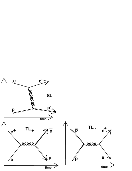
Fig. 1: Reactions (13) (labeled as SL in the figure), (13) (TL₊), (13) (TL_-). In the one photon exchange approximation, electromagnetic FFs are functions characterizing the vertex coupling the virtual photon to the hadron current (thick grey dashed line in the figure).

I.1 Effective proton timelike form factor - leading trend

The experimental and theoretical investigations of the TLFF are less advanced than for the spacelike (SL) case. In particular, the experimental separation of the electric and the magnetic FF has not been possible in the TL region, because of the available limited luminosity. The precision on the cross section $\sigma$ of the reactions (2,3) has only allowed for the extraction of the squared modulus of a single effective FF, $F_{p}$, that for reaction 2 is defined as Bardin et al. (1994):

$$|F_{p}|^{2}=\displaystyle\frac{3\beta q^{2}\sigma}{2\pi\alpha^{2}\left(2+\displaystyle\frac{1}{\tau}\right)},$$ (4)

where $\alpha=e^{2}/(4\pi)$, $\beta=\sqrt{1-1/\tau}$, $~{}\tau={q^{2}}/(4M^{2})$, $q^{2}$ is the squared invariant mass of the colliding pair, and $M$ is the proton mass. For reaction (3) we have a small difference in the definition of effective FF in terms of $\sigma$ (the final state phase space is not present anymore). The effect of the Coulomb singularity of both cross sections at the $\bar{p}p$ threshold is removed by the $\beta$ factor: $\beta$ $\rightarrow$ 0 for $q$ $\rightarrow$ $2M$, so that $\beta\sigma$ is finite and the effective FF is expected to be finite at the threshold.

This effective TLFF has been measured by several experiments for $q^{2}$ ranging from the threshold $(2M_{N})^{2}$ to about 36 GeV². In Fig. 2 the most recent and precise results are reported, from the Babar Lees et al. (2013a, b) and BES III collaborations Ablikim et al. (2015). These data have been fitted by some parameterizations. Four of them are reported in the figure. Details about these fits and the best fit values of their parameters can be found in our previous work Bianconi and Tomasi-Gustafsson (2016). The most visible feature is a strong power-law fall at increasing $q$. For example, in the experimental papers before the year 2006, the simple function Ambrogiani et al. (1999); Lepage and Brodsky (1979):

$$|F_{scaling}(q^{2})|=\displaystyle\frac{\cal A}{(q^{2})^{2}\log^{2}(q^{2}/\Lambda^{2})}$$ (5)

was frequently used, suggesting a $1/q^{4}$ trend apart for logarithmic corrections. The TLFF data from the BABAR collaboration Lees et al. (2013a, b) extending from the threshold to $q^{2}$ $\approx$ 36 GeV², look even steeper than this.

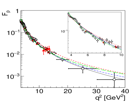
Fig. 2: Most recent data on the TL proton generalized FF as a function of $q^{2}$, from Ref. Lees et al. (2013a, b) (black open circles), Refs. Ablikim et al. (2005) (red triangles), together with the calculation from Eq. (5) (blue dash-dotted line, from Ambrogiani et al. (1999); Lepage and Brodsky (1979)), and from Shirkov and Solovtsov (1997); Kuraev (2008) (red dashed line), Brodsky and de Teramond (2008) (green long-dashed line), and Tomasi-Gustafsson and Rekalo (2001) (black solid line).

I.2 Modulation of the leading trend

For $q<$4 GeV the data also show oscillating 10 % modulations around this regular trend. In our works Bianconi and Tomasi-Gustafsson (2015, 2016) we have fitted the BABAR data with

$$F(p)\ \equiv\ F_{0}(p)\ +\ F_{osc}(p),$$ (6)

where $p=p(q)$ is the relative three-momentum of the final hadron pair, $F_{0}(p)$ is a standard fit expressed in terms of $p(q)$, and the modulation term $F_{osc}(p)$ is parameterized as

$$F_{osc}(p)\ \equiv\ A\ e^{-Bp}\ \cos(Cp\ +\ D).$$ (7)

The precise values of the parameters depend on the fit that is chosen as leading term $F_{0}$ (see Bianconi and Tomasi-Gustafsson (2016) for the four different choices). In all cases $A$ has magnitude $\simeq 0.1$, and $D$ $\approx$ 0. The smallness of $A$ suggests that the oscillations are due to some perturbation of a “leading” physics connected to the term $F_{0}$. $D$ $\approx$ 0 is an indication that the first oscillation is also a threshold enhancement, like those found in $e^{+}e^{-}\rightarrow\bar{n}n$, $e^{+}e^{-}\rightarrow\bar{\Lambda}\Lambda$ and other production processes of neutral baryon pairs Ablikim et al. (2010); Pakhlova et al. (2008); Ablikim et al. (2006, 2004); Bai et al. (2003); Amsler et al. (1994).

I.3 Hard and soft physics

At large $q^{2}$ things should simplify: the correction $F_{osc}$ should disappear, and $F_{0}$ should converge to the quark counting rules: TLFF $\propto$ $1/q^{4}$ (with logarithmic corrections), as for the case of the SLFF asymptotic Matveev et al. (1973); Brodsky and Farrar (1973). However, soft processes are expected to heavily affect the finite-$q$ deviations from the $1/q^{4}$ rule and to determine both the FF magnitude and phase not predictable by the quark counting rules. This has prompted several studies of the nonperturbative aspects of the TLFF and/or models for them and/or approaches to measurements Brodsky and de Teramond (2008); Gousset and Pire (1995); Bijker and Iachello (2004); Adamuscin et al. (2005); Belushkin et al. (2007); Lomon and Pacetti (2012); Bianconi et al. (2006a, b); Gakh and Tomasi-Gustafsson (2005, 2006); de Melo et al. (2004, 2006); Kuraev et al. (2012).

These studies were targeted at the leading features of the data shown in Fig. 2, the “regular” behavior reproduced by $F_{0}$. Concerning the 10% oscillations of Eqs. (6-7), there are interpretations proposed by us Bianconi and Tomasi-Gustafsson (2015, 2016) and by Lorenz et al. (2015), but this feature of the TLFF is still poorly explored.

As observed, the first oscillation is a threshold enhancement. This phenomenon has been studied in the electroproduction of neutral hadron pairs, where it is more evident. In Ref. Haidenbauer et al. (2014) an explanation in terms of nucleon-antinucleon strong-force potentials is proposed. Ref. Baldini et al. (2009) focusses on local electric interactions between quarks and antiquarks of the two baryons. This is equivalent to a reciprocally induced electric polarization of the interacting spin-1/2 hadron and antihadron, a mechanism that has also been also used in Ref. Bianconi et al. (2014) to explain enhancements of the low-energy rates for processes involving antineutrons. Whether is electrostatic or strong, in all cases what is suggested is an interaction between hadrons (hadron-antihadron potentials) just before their annihilation or just after their creation.

I.4 Antiproton-nucleon interactions

Interactions between a nucleon and an antinucleon are by themselves an important subject of nuclear physics. In particular data on the $\bar{p}$-nucleon and $\bar{p}-$nucleus annihilation process at low energies (see Balestra et al. (1986, 1989); Bizzarri et al. (1974); Bruckner et al. (1990); Balestra et al. (1984, 1985); Bertin et al. (1996); Benedettini et al. (1997); Zenoni et al. (1999a, b); Bianconi et al. (2000a, b); Bianconi et al. (2011); Aghai-Khozani et al. (2018)) and on antiprotonic nuclei Trzcinska et al. (2001), as well as related theoretical analyses Bruckner et al. (1990); Bianconi et al. (2000c); Batty et al. (2001); Friedman (2014); Lee and Wong (2016); Wycech et al. (2007); Uzikov et al. (2011) show that:

(a) Annihilation cross sections are large taking the unitarity limit as a reference. This means that in some partial waves a relevant part of the incoming projectile flux disappears in the interaction process: the proton is a black-sphere absorber for an antiproton flux, at any energy. Elastic scattering is present, mainly of diffractive origin (for momenta over 100-200  MeV/c), and of refractive repulsive hard-core nature near threshold or just below it (antiprotonic atoms). This repulsive character is an indirect consequence of the large absorption, and not of a repulsive potential: the need of a regular behavior of the wave function at the border of the region where it is suppressed by absorption determines a strong reflected component.

(b) A proton and an antinucleon do not overlap. When their surfaces come in touch a quark from the proton and an antiquark from the antiproton easily rearrange into a meson leaving an unstable system followed by annihilation into multi-meson states. This clearly hinders the chances that three quarks and three antiquarks may gather in a region of size $1/q$ (0.1 fm at threshold), that is a precondition for converting all of them into a single lepton pair. The same problem is present in the reverse process of $\bar{p}p$ production, since the two hadrons should be created in a configuration where their chance to exist is very small.

(c) The available data on low-energy $\bar{p}p$ processes are normally described in terms of optical potential analyses within a non-relativistic formalism.

I.5 Aim of the present work

In a previous publication Bianconi and Tomasi-Gustafsson (2017) we discussed the physics of the proton TLFF in spacetime. In the SL case the FFs in the Breit frame ($q_{0}=$ 0, no energy transfer) are interpreted as Fourier space transforms of stationary charge and current distributions. We studied a corresponding interpretation for the timelike FF in the CM frame of the $e^{+}e^{-}$ collision where the photon has zero three-momentum (infinite space wavelength). What one finds is a distribution in time of the photon-quark-antiquark creation vertexes. Such distribution and the space charge distribution are the projections respectively on the time axis and on the three-space of one and the same four-dimensional spacetime distribution $F(x)$.

For simplicity, we avoided the rescattering problem, since this is a broad subject and deserves a dedicated work. This is the subject of the present paper. We use the word “rescattering” to describe interactions between the hadrons both in reaction 2 and 3 where, strictly speaking, it should be defined as “pre-scattering”.

Since it may be ambiguous to decide which processes have to be classified as rescattering, a specific definition will be given in the next section. Let us anticipate that a special stress will be given to elastic rescattering, to charge exchange and to annihilation.

II Soft rescattering

In a previous work Bianconi and Tomasi-Gustafsson (2016) we introduced the role of rescattering in TLFFs, where an optical potential model was used to explain the oscillations of the effective proton TLFF above threshold. A basic assumption of that work was that rescattering was a small perturbation, while the most evident behavior of the FF (a very fast but regular decrease at increasing $q$) was due to a “leading” mechanism. The purely phenomenological background for this was the fact that the oscillations did not exceed 10 % of the FF absolute value. Since the same “smallness” assumption will accompany all of the present work, we better need to define what we mean by “small”, by “leading”, and by “rescattering”.

There is no easy way here to split the interaction Hamitonian into a form like $V$ $=$ $V_{F}$ $+$ $V_{R}$ where separate terms are responsible for hadron formation and rescattering between physical hadrons. The only exception is when “rescattering” means Coulomb interaction between the final or initial hadrons, but we are interested in a broader class of phenomena, involving strong interactions.

Within a perturbative and convergent scheme, the complete amplitude for a process like $e^{+}e^{-}$ $\rightarrow$ $\bar{p}p$ is a sum of a “bare” formation process plus an infinite set of amplitudes including rescattering events, as described in Fig. 3. This derives from the Born series expansion of the exponential that formally expresses the effect of the interaction potential: $exp(i\int Vdt)$ $=$ $1$ $+$ $T\int iVdt^{\prime}$ $+$ $T\int(iV)^{2}/2dt^{\prime}dt^{\prime\prime}$ $+$ $...$. So, when a perturbative scheme is available rescattering just means a class of higher order processes.

Here a rapidly converging perturbative scheme is not available. Although much of the involved interactions can be treated within theories like PQCD or VDM, hard and soft strong interactions cannot be framed within one and the same perturbative scheme, and both are heavily involved in the pair formation process.

To simplify our problem, and taking into account that our research line focusses on subleading behaviors, in the present work “rescattering” only means “soft rescattering between physical hadrons”.

To distinguish hard from soft processes, the point is not the nature of the involved particles (quarks vs hadrons, for example) but their offshellness. Even a model based on hadrons describes hard physics if the offshellness of these hadrons is hard-scaled. So, processes involving far-off-shell propagators are excluded from what we mean by rescattering.

The “bare formation” of hadrons implies both hard and soft processes, as evident in the very basic and well known scheme where the reaction $e^{+}e^{-}\to\bar{p}p$ requires first the formation of three $\bar{q}q$ pairs within a $1/q$-sized region via perturbative quantum chromodynamics (PQCD) hard processes, but then each subgroup of three quarks and three antiquarks must evolve toward a physical hadron configuration with a much larger radius, and this evolution is non-perturbative and soft. In this path we have an “unavoidable” rescattering: after the first one, two more $\bar{q}q$ pairs are formed, and this cannot take place without involving both forming hadrons. Here to speak of rescattering as something distinguished from the formation process is nonsense. So, everything that takes place in this stage is not rescattering.

Starting from the time when two separate color singlets may be identified, further interactions between the two become “avoidable”. That is, they will take place with some frequency, but a proton and an antiproton can be formed in their absence too. If in some “avoidable” rescattering the involved propagators are highly virtual, the two steps of $\bar{q}q$ formation and rescattering are within $1/q$ in spacetime and even in this case difficult to conceptually disentangle.

Those “avoidable” processes that involve only soft propagators take place on a larger spacetime scale and in this approximate sense they may be distinguished from the “formation” processes. Because of the longer involved wavelengths, these processes involve hadrons rather than individual quarks.

The last relevant point is that soft steps are also heavily involved in the formation processes of the individual hadrons. We assume that on a time scale $\gg 1/q$ it is possible :

a) to identify two color singlets that, although are not yet a proton and an antiproton, will separately evolve into them;

b) to distinguish the intra-singlet from the inter-singlet processes.

Summarizing, those “avoidable” processes that are soft and may be classified as interaction between singlets are what we mean with “soft rescattering”.

This is illustrated in Fig. 3, where the full amplitued is shown as the sum of a “bare formation” amplitude and of processes where the bare formation (the first blob on the left) is followed by further interaction. The legs on the right of the bare formation blob are near-on-shell hadrons. Those rescattering processes that involve hadrons or quarks with virtuality $\sim$ $q$ are considered as a renormalization of the bare formation amplitude, and not rescattering, and so, in Fig. 3 they are hidden inside the formation blob.

So, for example a VDM “bare” process like $e^{+}e^{-}\rightarrow M^{*}\rightarrow\bar{p}p$, where $M^{*}$ is a vector meson that is highly offshell in the physical $\bar{p}p$ channel, has rescattering corrections like $e^{+}e^{-}\rightarrow M^{*}\rightarrow\bar{p}p\rightarrow M^{*}\rightarrow\bar{p}p$. Such a correction is not considered as “rescattering” in this work, since it involves a meson with a hard-scale virtuality. We consider the terms like this as a renormalization of the hard part of the TLFF. On the other side, in a process like $e^{+}e^{-}\rightarrow M^{*}\rightarrow\bar{n}n\rightarrow\bar{p}p$ the final state charge exchange $\bar{n}n\rightarrow\bar{p}p$ is definitely “soft rescattering” in our interpretation if it is due to the $t-$channel exchange of a pion. The same is true for diffractive scattering mediated by a $t-$channel pomeron.

In particular, we consider potential scattering as soft, even in the special case of an optical potential. An optical potential averages $\bar{p}p$ interactions that can be highly inelastic into an energy-conserving interaction that produces regular changes of the $\bar{p}p$ wave function (neglecting the effects on the other channels, and averaging irregularities over a finite energy range). So it describes soft effects of processes that can be hard.

Rescattering allows for the presence of a Cutkowsky cut in the diagram for the photon-hadron vertex (see Fig. 4). This cut implies an imaginary part in the FF if it intercepts a state that may be physical at the considered kinematics. As evident from Fig. 4, such a cut may be present on the propagators of the hadrons in the intermediate state, but it may also cut the bare formation blob, since this hides hard rescattering processes. So an imaginary part may be already present in the “bare” TLFF, but it surely receives contributions from hadronic states in presence of soft rescattering. In particular one may expect that an optical potential interaction contributes to the imaginary part of a FF. This point will be discussed at the end of this work.

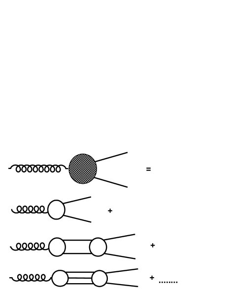
Fig. 3: Amplitude for the formation of a $\bar{p}p$ pair as a sum of a “bare” amplitude plus rescattering corrections. These are of two kinds: elastic rescattering (that may be iterated 1, 2, … times) and inelastic rescattering, with several possible intermediate states. In the present work we assume that the “bare” amplitude is actually a partially resummed amplitude calculated within some model, including all those rescattering processes that may be considered as hard, and all those soft processes that take place within the 3$q$ color singlet or within the 3$\bar{q}$ singlet and do not involve singlet-singlet interactions. We consider as “rescattering” only those soft singlet-singlet interactions involving near-on-shell hadrons.

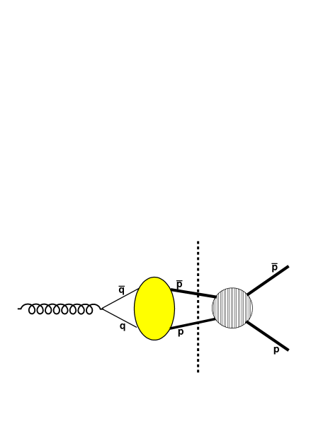
Fig. 4: Process with initial formation of a quark-antiquark pair, then converted into a hadron pair according to a “bare” FF (left blob). The hadron pair interacts again (right blob, that may be t-channel or s-channel rescattering), and this adds a subleading correction to the FF. A cut on a physical state is possible in the intermediate di-hadron state, leading to an imaginary part of the FF. If the left blob contains physical intermediate states, then it may be crossed by another cut, and this will produce an imaginary part in the “bare” FF. If the rescattering blob is of s-channel kind, e.g. with formation of a single meson, the rescattering blob may be cut as well. So, several cuts are possible, but this work focusses on the cuts like the one showed here.

III Four-dimensional Fourier transform of the FF

The key tool for the investigation of FFs is the four-dimensional Fourier transform Kuraev et al. (2012)

$$F(q)\ =\ \int d^{4}xe^{iqx}F(x).$$ (8)

Although $F(q)$ may be analyzed as a function of $q^{2}$ on all the complex plane, here we consider it as a function of all the 4 components of $q_{\mu}$, since the Fourier transform is separately performed with respect to each of them. So, in the following $x$ and $q$ mean $x_{\mu}$ and $q_{\mu}$. From a physical point of view, $F(x)$ is the amplitude $F(q)$ in another representation, that is the 4-position of the photon-current vertex instead of the photon 4-momentum.

Although FFs are normally introduced as pieces of an amplitude, they may be considered amplitudes themselves. We need to distinguish between “resolvable” and “unresolvable” particles, as in Fig. 5. A resolvable particle participates to a process with its internal structure, while an unresolvable particle is treated as elementary. As an unresolvable particle, the photon-hadron current interaction takes place in a single vertex $X_{\mu}$. At a resolvable level the photon-hadron interaction involves several variables $X_{1}^{\mu},X_{2}^{\mu},...$ associated to the internal hadron constituents (we omit the tensor indexes and just write $X$, $X_{1}$ etc). In particular let $X_{1}$ be the 4-position where the photon couples with an elementary (quark) current.

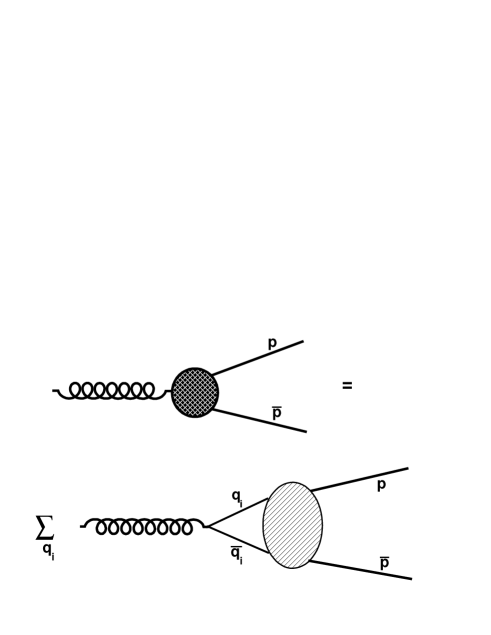
Fig. 5: Unresolved and resolved level of analysis (see text), within a quark model. The TLFF in 4-coordinate representation $F(x)$ is a sum of amplitudes for converting a quark-antiquark pair that has been created in a 4-point into a proton-antiproton pair created in another 4-point, where $x$ $\equiv$ $x_{\mu}$ is the 4-distance of the two points. For the opposite process ($\bar{p}p$ annihilation into a virtual photon) it is an amplitude for finding a $\bar{q}q$ pair in a 4-point given a $\bar{p}p$ pair in another 4-point.

In coordinate representation, a FF $F(x)$ is the amplitude for the photon coupling taking place in a given 4-point $X_{1}$ at resolvable level, if the photon coupling at unresolvable level takes place in another point $X$, with $x=X_{1}-X$. Then of course things are made more complicate by the presence of more form factors entering a process, and by the fact that more $\bar{q}q$ pairs may couple with the photon. But this does not change the interpretation of a FF as an amplitude for seeing a hadron current at a deeper resolution level.

In the SL case, and in the Breit frame where $q^{\mu}=(0,\vec{q})$, the known non-relativistic interpretation of a form factor holds:

$$F_{SL,Breit}(q)\ =\ \int d^{3}\vec{x}\ exp(-i\vec{q}\cdot\vec{x})\int dtF(t,\vec{x})\ \equiv\ \int d^{3}\vec{x}\ exp(-i\vec{q}\cdot\vec{x})\rho(|\vec{x}|)$$ (9)

$$\rho(|\vec{x}|)\ =\ \int dtF(t,\vec{x}).$$ (10)

where $\rho(|\vec{x}|)$ may be read as a static charge density. Here it appears as a time average over the Fourier transform $F(x)$ $=$ $F(t,\vec{x})$.

In the TL case, and in the center of mass frame ($\vec{q}$ $=$ 0) we have a corresponding interpretation:

$$F_{TL,CM}(q)\ =\ \int dt\ exp(iqt)\int d^{3}\vec{x}F(t,\vec{x})\ \equiv\ \int dt\ exp(iqt)R(t),$$ (11)

$$R(t)\ =\ \int d^{3}\vec{x}F(t,\vec{x}).$$ (12)

It must be observed that in neither case one may access $F(x)$. Either one explores $\rho(\vec{x})$ or $R(t)$, that are integrals of $F(x)$. So measuring TL and SL FFs leads to complementary pieces of information.

IV The no-rescattering case.

The reactions from which the TL and the SL FFs are extracted are related by crossing symmetry (see Fig. 1). The one-photon exchange mechanism is assumed, so in the following “FF” stays for a renormalizing factor for the hadron-virtual photon vertex, as in Fig. 6. Factorizing out the lepton part of the process and the virtual photon propagation, we only consider the three-leg amplitude $A(q,P_{A},P_{B})$ describing the sub-processes

$$SL: \ \gamma^{*}(q_{\mu})\ +\ p(p_{\mu})\rightarrow p(p_{\mu}^{\prime}),$$ (13)

$$TL_{+}: \ \gamma^{*}(q_{\mu})\ \rightarrow p(p_{\mu}^{\prime})\ +\ \bar{p}(\bar{p_{\mu}}^{\prime}),$$ (14)

$$TL_{-}: \ p(p_{\mu})\ +\ \bar{p}(\bar{p}_{\mu})\ \rightarrow\gamma^{*}(q_{\mu}^{\prime}).$$ (15)

The four-momenta $q^{\mu}$, $P_{A}^{\mu}$, $P_{B}^{\mu}$ appearing as $formal$ arguments of $A(q,P_{A},P_{B})$ are all incoming as in Fig. 6 so that the different reactions are distinguished by the expression of $q$, $P_{A}$ and $P_{B}$ in terms of the $physical$ momenta $q$, $q^{\prime}$, $p$, $p^{\prime}$, $\bar{p}$, $\bar{p}^{\prime}$ (that have a positive time component if they are timelike):

$$\gamma^{*}+p\rightarrow p^{\prime}\hskip 28.45274pt(SL:\ |q_{0}|\ <\ |\vec{q}|)\ P_{A}\ =\ p,\ P_{B}\ =\ -p^{\prime},$$ (16)

$$\gamma^{*}\rightarrow\bar{p}+p\hskip 28.45274pt(TL_{+}:\ |q_{0}|\ >\ |\vec{q}|,\ q_{0}\ >\ 0)\ P_{A}\ =\ -p^{\prime},\ P_{B}\ =\ -\bar{p}^{\prime}.$$ (17)

$$\bar{p}+p\rightarrow\gamma^{*}\hskip 28.45274pt(TL_{-}:\ |q_{0}|\ >\ |\vec{q}|,\ q_{0}\ <\ 0)\ P_{A}\ =\ p,\ P_{B}\ =\ \bar{p},\ q\ =\ -q^{\prime}.$$ (18)

where in the TL region two reciprocally inverse reactions are possible, corresponding to $\bar{p}p$ annihilation into or creation from a lepton-antilepton pair.

It is important not to confuse the four-momenta $P_{A}$ and $P_{B}$ as formal arguments of $A$, with their physical values $\pm p$, $\pm\bar{p}$…: the analytical continuation of $A(q,P_{A},P_{B})$ requires that this amplitude is described in terms of the same arguments in all the reaction channels and in the nonphysical regions (so, $q_{0}$ $<$ 0 in one of the two annihilation channels, and it is a complex variable in general). Being $A(q,P_{A},P_{B})$ invariant, it actually depends on $q$, $P_{A}$ and $P_{B}$ via their invariant products only, so these three four-vectors contain redundant information. However, in the following we keep the formal dependence of $A$ on them.

Assuming a muon as a template for an unresolvable proton, $i.e.,$ a “pointlike” proton, the vertex matrix element for $\gamma(q)$ $+$ $\mu(p)$ $\rightarrow$ $\mu(p^{\prime})$ is (using $\bar{u}\gamma^{0}$ $=$ $u^{+}$)

$$A_{point\ SL}(q,p,p^{\prime})\ =\ <\mu^{\prime}|A_{\nu}(X)J^{\nu}(X)\ |\mu>\ =\ e\int d^{4}X\ e^{iqX}\ e^{-ip^{\prime}X}\ e^{ipX}\ e_{\nu}\ \bar{u}(p^{\prime})\gamma^{\nu}u(p)\ =\$$ (19)

$$=\ e\int d^{4}Xe^{iqX}e^{-ip^{\prime}X}e^{ipX}\Big{(}e_{0}\ u^{+}(p^{\prime})u(p)\ -\ \vec{e}\ \bar{u}(p^{\prime})\vec{\gamma}u(p)\Big{)}\ =$$ (20)

$$=\ \delta^{4}(q+p-p^{\prime})\ \Big{(}T_{point\ charge}(q,p,p^{\prime})\ -\ T_{point\ current}(q,p,p^{\prime})\Big{)}.$$ (21)

Exploiting that the amplitudes of the processes (17) and (18) are analytical continuations of the amplitude of (16), we can write Eq. (21) in a compact form describing all these processes:

$$A_{point}(q,P_{A},P_{B})\ \equiv\ \delta^{4}(q+P_{A}+P_{B})\ \Big{(}T_{point\ charge}(q,P_{A},P_{B})\ -\ T_{point\ current}(q,P_{A},P_{B})\Big{)}.$$ (22)

where assigning to $q$, $P_{A}$, $P_{B}$ the values listed in Eqs. (16,17,18), we obtain the amplitudes for the corresponding reactions.

Form factors may be introduced as scalar functions that multiply the previous terms, or linear combinations of these terms:

$$A(q,P_{A},P_{B})\ \equiv\ A_{charge}(q,P_{A},P_{B})\ -\ A_{current}(q,P_{A},P_{B})$$ (23)

$$\equiv\ \delta^{4}(q+P_{A}+P_{B})\ \bigg{(}T_{point\ charge}(q,P_{A},P_{B})\ F(q)\ -\ T_{point\ current}(q,P_{A},P_{B})\ G(q)\bigg{)}$$ (24)

where now this amplitude describes processes involving proton and antiproton instead of muons. The scalar FFs $F(q)$ and $G(q)$ depend on $q_{\mu}$ via the scalar $q^{2}$ $\equiv$ $q_{\mu}q^{\mu}$ only. Alternatively, one may rewrite the hadron four-current in the Gordon form, insert $F_{1}$ and $F_{2}$ and next combine them into $G_{E}$ and $G_{M}$, but the adopted procedure is simpler since it immediately highlights the term that is proportional to the charge density operator $u^{+}(p^{\prime})u(p)$, and we will not work on the other component in the following.

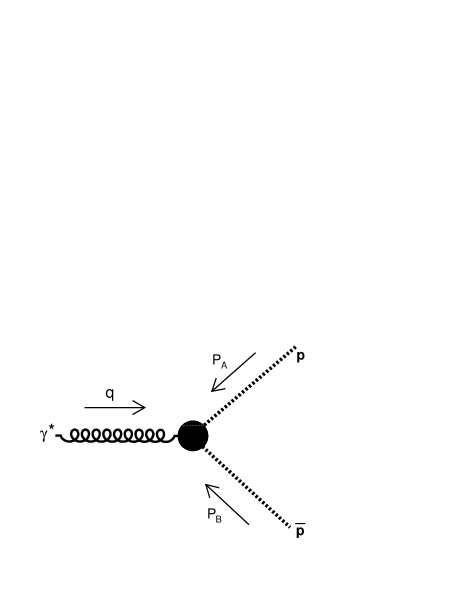
Fig. 6: Diagram describing the three reactions (16, 17, 18). Since these are actually physical channels of the same reaction, all of them may be described by the same diagram and by the same amplitude by changing the values of the components of the four-momenta $P_{A}$, $P_{B}$, $q$ and exploiting crossing symmetry. Formally, we consider these momenta as all entering. So, $q$ coincides with the physical four-momentum of the virtual photon in the channel $TL_{+}$ where a $\bar{p}p$ pair is created, while $q$ $=$ $-q^{\prime}$, where $q^{\prime}$ is the physical four-momentum of the virtual photon, in the reverse channel $TL_{-}$ where a virtual photon is produced by $\bar{p}p$ annihilation. Similar considerations apply to $P_{A}$ and $P_{B}$, see Eqs. (16,18), for all the correspondences between formal arguments of the amplitude and physical momenta).

Our further analysis only considers the FF $F(q)$ associated with the charge term. So our starting equation is:

$$A_{charge}(q,P_{A},P_{B})\equiv\ \delta^{4}(q+P_{A}+P_{B})\ T_{point\ charge}(q,P_{A},P_{B})\ F(q)$$ (25)

V Translation invariance and Inner degrees of freedom.

We consider here the FF in a quark model framework, where it is assumed that the process of $\bar{p}p$ creation or annihilation is built around a quark-antiquark creation by the photon, or quark-antiquark annihilation into a photon, and several additional degrees of freedom enter the process, for example spectator quark coordinates.

The amplitude describing how a $free$ (anti)proton with momentum $p$ splits into a Fock state of $N$ constituents is

$$\psi(X_{1},X_{2},....X_{N})\ \equiv\ e^{ipX}\Phi(x_{1},x_{2},...x_{N})$$ (26)

where the four-vector $X_{i}$ is the spacetime position of the i-th constituent, $X$ is a linear combination of all the $X_{i}$, expressing the spacetime position of the proton as a whole (the unresolved proton) and the four-coordinates $x_{i}$ are internal four-coordinates relative to $X$:

$$X\ =\ \sum w_{i}X_{i},\ i=1,....N.$$ (27)

$$x_{i}\ \equiv\ X_{i}-X.$$ (28)

$$\sum\ w_{i}x_{i}\ =\ 0,$$ (29)

where $w_{i}$ are weights that depend on dynamics (for example, on the longitudinal fractions or on the mass) within a given model.

A key point is that because of spacetime translation invariance, a separation between relative and absolute coordinates leading to the factorization (26) must exist, at the condition that the proton as a whole does not interact with the surrounding environment. This prerequisite is not present anymore if we introduce rescattering, that in our case means interactions between the proton and the antiproton before their annihilation or after their creation. Of course, an isolated set of particles may always be identified, unless very long range forces are included. This will lead to the separation of a degree of freedom that enjoys translational invariance.

We now consider first a diagram contributing to the FF in absence of rescattering, as in Fig. 7. So, $\Phi$ is a splitting amplitude for a free proton, and is a fully relativistic amplitude, where each four-coordinate has an independent time dependence.

Let us assume that the vitual photon creates a $\bar{p}p$ pair in a non interacting state. So, this state is described by the product $\psi^{+}(X_{1},X_{2},...)\ Q(X_{1},X_{2},...)\psi^{\prime}(X_{1},X_{2},...)$ where $\psi$ refers to the proton, $\psi^{\prime}$ to the antiproton $X_{1}$ is the four-point where the first $\bar{q}q$ pair is directly created by the photon, $X_{2}$ the four-point where the second pair is created and so on. $Q$ is a kernel describing the $hard$ dynamic steps leading from the first pair to the other ones (as in PQCD where a gluon radiated from a quark splits into another pair). It may only depend on the relative positions $x_{i}$ of the pair creation points. Since we have requested that the final state is a non-interacting one, soft processes are all factorizable for the time being, that is, they take independently place inside $\Phi$ or $\Phi^{\prime}$.

We may rewrite Eq. (25) for the process $\gamma^{*}$ $\rightarrow$ $\bar{p}p$ as:

$$A_{TL,charge}\ =\ R_{point,charge}(q,p,\bar{p})\ e_{1}\int dX_{1}dX_{2}....exp(iqX_{1})\psi^{+}(X_{1},X_{2},...)\ Q(X_{1},X_{2},...)\psi^{\prime}(X_{1},X_{2},...)\ =$$ (30)

$$=\ R_{point,charge}(q,p,\bar{p})\ e_{1}\int dXexp[i(q-p-\bar{p})X]\int dx_{1}exp(iqx_{1})\int dx_{2}...\delta^{4}(\sum w_{i}x_{i})$$

$$\Phi^{+}(x_{1},x_{2},...)\ Q(x_{1},x_{2},...)\Phi^{\prime}(x_{1},x_{2},...)\ \equiv$$ (31)

$$\equiv\ R_{point,charge}(q,p,\bar{p})\ \delta^{4}(q-p-\bar{p})\ \int d^{4}x_{1}exp(iqx_{1})F(x_{1}),\hskip 14.22636ptx\equiv\ x_{1}.$$ (32)

This is simply summarized in Fig. 7, where the virtual photon wave is $exp(iqx_{1})$ and the blob in $X$ with two legs reaching $X_{1}$ $\equiv$ $X+x_{1}$ is the form factor $F(x_{1})$ , that we interpret as an amplitude for finding a $\bar{q}q$ pair in $x_{1}$ resolved level) given a $\bar{p}p$ pair in $X$ (unresolved level).

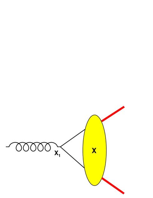
Fig. 7: Diagram corresponding to Eq. (32). The four-coodinate where the hadron pair is formed/annihilated (timelike process) or where the hadron is scattered (spacelike process) is $X$. At resolved level, the coordinate where the $\bar{q}q$ pair is formed/annihilated (TL), or where a quark is scattered (SL) is $X_{1}$. The electromagnetic FF quantifies the effect of the photon probe on the degree of freedom $x_{1}$ $\equiv$ $X_{1}-X$.

VI Soft rescattering

Let us now consider the t-channel exchange of an interaction quantum between the final hadrons, as in Fig. 8. Rescattering is not necessarily elastic, so the hadrons that are produced before rescattering do not necessarily coincide with a proton and an antiproton. However, since we require the rescattering to be soft, the intermediate state cannot consist of, say, three pions or a vector meson. Near threshold, the only cases that may be admitted are intermediate states formed by a nucleon-antinucleon pair plus possibly one pion. At large $q$ we may have near-physical states including a baryon-antibaryon pair. We now discuss an example with an intermediate hadron pair.

The initial hadron and antihadron states are created in $X$. Let $G(X,X^{\prime\prime})$ and $G^{*}(X,X^{\prime\prime\prime})$ be the two-point amplitudes describing the propagation of these intermediate-state hadrons to the vertexes $X^{\prime\prime}$ and $X^{\prime\prime\prime}$. The amplitude $B(X^{\prime\prime}-X^{\prime\prime\prime})$ describes the exchange of an interaction between the two.

Starting from the previous no-rescattering case, we must substitute the final state wavefunction $e^{i(p+\bar{p})X}$ with a block including the intermediate-state propagations, the interaction, the new final state wavefunction:

$$e^{i(p+\bar{p})X}\ \rightarrow\int d^{4}X^{\prime\prime}d^{4}X^{\prime\prime\prime}G(X-X^{\prime\prime})G^{*}(X-X^{\prime\prime\prime})B(X^{\prime\prime}-X^{\prime\prime\prime})e^{-ipX^{\prime\prime}}e^{-i\bar{p}X^{\prime\prime\prime}}$$ (33)

We apply the variable separation:

$$X_{R}\ \equiv\ (X^{\prime\prime}+X^{\prime\prime\prime})/2$$

$$\Delta\ \equiv\ X^{\prime\prime}-X^{\prime\prime\prime}$$

$$Y\ \equiv\ X_{R}-X.$$ (34)

$Y$ is the four-distance between the first hadron-antihadron formation point $X$ and the average rescattering position $X_{R}$ $=$ $(X^{\prime\prime}+X^{\prime\prime\prime})/2$. So, to further develop Eqs. (30-32) we use

$$e^{iqx_{1}}\ =\ e^{-iqx}e^{iqX}\ =\ e^{-iqx}e^{iq(Y+X_{R})},$$ (35)

$$e^{ipX^{\prime\prime}}\ =\ e^{ip(X+\Delta/2)},\ e^{i\bar{p}X^{\prime\prime\prime}}\ =\ e^{i\bar{p}(X-\Delta/2)},$$ (36)

$$G(X^{\prime\prime}-X)\ =\ G(Y+\Delta/2),\ G^{*}(X^{\prime\prime\prime}-X)\ =\ G^{*}(Y-\Delta/2),$$ (37)

$$B(X^{\prime\prime}-X^{\prime\prime\prime})\ =\ B(\Delta).$$ (38)

The factor $\int d^{4}xe^{iqx}F(x)$ is formally untouched by the previous operations (although it may now refer to hadrons different from $p$ and $\bar{p}$) and we have

$$\int d^{4}Xd^{4}X^{\prime\prime}d^{4}X^{\prime\prime\prime}....\ =$$

$$\int d^{4}X_{R}e^{i(q-p-\bar{p})X_{R}}\ \int d^{4}Ye^{iqY}\ \Bigg{(}\int d^{4}\Delta G(Y+\Delta/2)G^{*}(Y-\Delta/2)B(\Delta)\ \Bigg{)}.$$

The amplitude that replaces Eq. (32) is

$$A(q)\ =\ \delta^{4}(q-p-\bar{p})\ R_{point\ charge}(q)\ F_{0}(q)\ F_{R}(q),$$ (40)

where $F_{0}(q)$ is the no-rescattering FF corresponding to the creation of the hadrons of the intermediate state, and rescattering is described by

$$F_{R}(q)\ \equiv\ \int d^{4}Y\ e^{iqY}\ \int d^{4}\Delta G(Y+\Delta/2)G^{*}(Y-\Delta/2)B(\Delta).$$ (41)

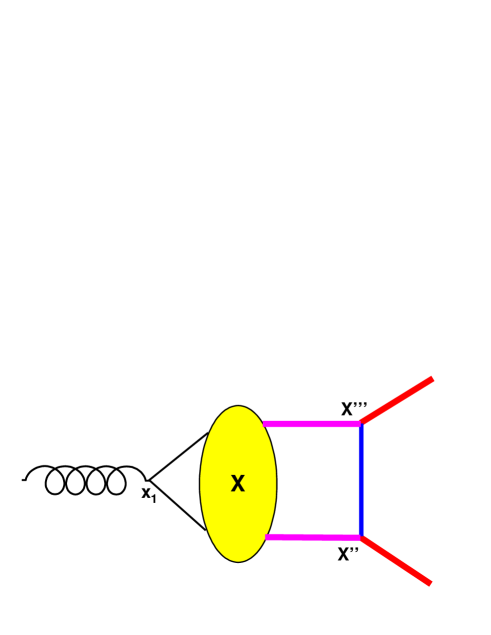
Fig. 8: TLFF including t-channel rescattering between the final hadrons.

Fig. 8 may describe the two-step process $\gamma^{*}$ $\rightarrow$ $\bar{p}p$ $\rightarrow$ $\bar{p}p$, but may also describe a process like $\gamma^{*}$ $\rightarrow$ $\bar{n}n$ $\rightarrow$ $\bar{p}p$ where a charge exchange takes place in the second step. This process is quite likely near the threshold. At larger $q$, other processes with two hadrons in the intermediate state are possible, or with two hadrons and some meson.

Therefore, near threshold we could sum over three diagrams: direct production as in Fig. 7: elastic rescattering and $\bar{n}n$ intermediate state and we may write:

$$A(q)\ =\ \delta^{4}(q-p-\bar{p})\ R_{point\ charge}(q)\ \Bigg{(}F_{0,p}(q)\ \Big{(}1\ +\ F_{R,diag}(q)\Big{)}+\ F_{0,n}(q)\ F_{R,cex}(q),\ \Bigg{)}$$ (42)

where $F_{0,p}(q)$ is the no-rescattering FF for $\gamma^{*}$ $\rightarrow$ $\bar{p}p$, while $F_{0,n}(q)$ is the no-rescattering FF for $\gamma^{*}$ $\rightarrow$ $\bar{n}n$. $F_{R,diag}(q)$ and $F_{R,cex}(q)$ are the factors describing the effects of rescattering without and with charge exchange.

At larger $q$ more processes will need to be included:

$$A(q)\ =\ \delta^{4}(q-p-\bar{p})\ R_{point\ charge}(q)\ \Bigg{(}F_{0}(q)\ \Big{(}1\ +\ F_{R,diag}(q)\Big{)}+\ \sum_{i}F_{i}(q)\ F_{R,i}(q)\Bigg{)},$$ (43)

where the “i” terms take into account inelastic transitions proceeding through the intermediate hadron states $|i\big{>}$ formed in the early stages of the process by the amplitude $F_{i}(q)$. We remark that, although these states may be $BB^{*}$ with large mass baryons, here we are only summing over small-virtuality states, that able to propagate for a relatively long time.

VII Unitarity contribution: a strong imaginary part?

Actually the most relevant rescattering process is likely to be the one represented in Fig. 9, although it does not lead to a final $\bar{p}p$ state. Because of unitarity, this process removes $\bar{p}p$ pairs from the outgoing flux of the $\gamma^{*}$ $\rightarrow$ $\bar{p}p$ and from the incoming flux of the $\bar{p}p$ $\rightarrow$ $\gamma^{*}$ processes. So, we expect it to decrease, perhaps heavily, the TLFF, but more subtle and interesting properties can be predicted.

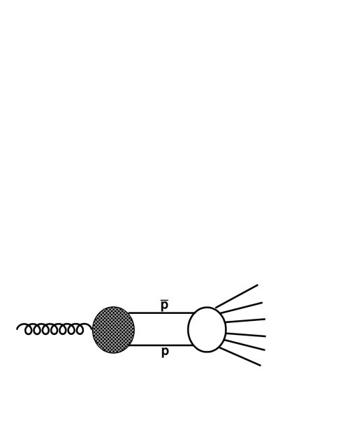
Fig. 9: Inelastic diagram of one of the many and frequent processes where the just created $\bar{p}p$ pair is lost because of later annihilation into several pions.

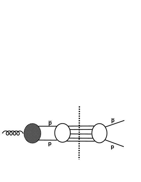
Fig. 10: Contribution of the $\bar{p}p$ annihilation processes to the imaginary part of the TLFF.

In the perturbative Born-style treatment of a process at the lowest order including interaction (as for the case of previous eq.43) each accessible final channel just adds itself to the overall cross section without disturbing the other channels, because the perturbative expansion is based on the requirement of small reaction amplitudes. Implicitly this smallness requirement implies that the incoming flux is so large that when we analyze a process we may neglect the flux depletion due to all the other ones. At higher order this inter-channel influence appears as an interference effect.

Evidently a first order perturbative expansion is suitable to small-amplitude processes where convergence is fast and higher orders are not decisive. When the amplitudes of different processes are so large to absorb a relevant portion of the incoming flux, they end up competing for this flux, so that each process reduces the cross section of the other ones. This is well visible in all those hadronic processes where we find a cross section minimum at an energy $E_{0}$ because of the competition with a channel that is resonant at $E_{0}$.

The inclusive cross section of the $\bar{p}p$ annihilation at relative momenta $\sim$ 10-1000 MeV/c is a relevant portion of the unitarity limit (that takes place when all the incoming flux is completely absorbed in a partial wavea). Since inelastic processes like those of Fig. 9 present a large cross section, they also give a large contribution to the imaginary part of the elastic $\bar{p}p$ $\rightarrow$ $\bar{p}p$ scattering, and so, indirectly, to the imaginary part of the $\gamma^{*}$ $\rightarrow$ $\bar{p}p$, due to the Cutkowsky cut that can be seen in Fig. 10.

To clarify this point, if $\bar{p}p$ annihilation saturated the unitarity limit, then the $\bar{p}p$ scattering amplitude would be completely imaginary (it would exactly coincide with the center of the Argand circle). Watson’s theorem Watson (1954) states that the phase of an amplitude leading to a final state with two strongly interacting particles in a given partial wave is the same as the scattering phase of that pair. So, near the threshold (pure S-wave) even the overall $\gamma^{*}$ $\rightarrow$ $\bar{p}p$ amplitude would be imaginary.

Writing the amplitude for $\gamma^{*}$ $\rightarrow$ $\bar{p}p$ as the amplitude for a “pointlike” process like $\gamma^{*}$ $\rightarrow$ $\mu^{+}\mu^{-}$ times the TLFF of the proton, and observing that the pointlike amplitude presents no special features, the imaginary character of the overall amplitude would entirely derive from an imaginary TLFF.

We cannot implement all what is known from the theory and the experiment concerning $\bar{p}p$ scattering and annihilation, because the TLFF only involves the vector component of the $\bar{p}p$ flux. However, the fact that the cross section for many-pion annihilation is large should be a common property of all the $\bar{p}p$ partial waves. So, we can consider some relevant results from the literature of $\bar{p}p$ interactions at small energies, associated with this property.

First, we know from theory and have experimental check from antiprotonic atoms that the real and the imaginary part of the scattering amplitude near the threshold are equal (this equality takes place in regime of S-wave dominance, that is between $p$ $=$ 0 and $p$ $\sim$ a few tenths of MeV/c corresponding to a relative energy $\approx$ 1 MeV). The inelastic cross section is large, but still far from the unitarity limit.

At $p\gtrsim 200$ MeV/c (relative energy $\gtrsim$ 40 MeV) an approximately eikonal regime is present, where the physics is essentially “black-sphere plus diffraction”. In this case $\bar{p}p$ scattering is mainly forward and imaginary-dominated, and the radius of the black sphere is of magnitude $simeq$ 1 fm and scarcely energy dependent. No resonances have ever been seen.

We can draw some hypotheses from this. In the eikonal regime ($p\gtrsim 200$ MeV/c) rescattering is relevant but cannot dominate the problem, because its geometrical cross section $<$ 100 mbarn $=$ 10 fm² (it tends to 50 mbarn at GeV energies) limits the probability that a proton and an antiproton rescatter, considering that we assume that “rescattering” takes place when the hadrons are distant at least 1 fm. On the other side, these numbers also mean that rescattering is present and not negligible at all. This black-disk rescattering implies regeneration of flux by diffraction of the same magnitude. So it does not decrease the TLFF, but rather shifts its phase. The regenerated flux presents a phase shift of $90^{\circ}$ with respect to the non-scattered flux. So, it introduces a relevant, although not dominant, imaginary part in the TLFF.

Near threshold, when the S-wave is relevant or dominant, one can apply Watson’s theorem and, as already observed, the TLFF must present the same phase features of the $\bar{p}p$ scattering amplitude, $i.e.$, equal real and imaginary parts.

VIII Time and distance in three-dimensional and non-relativistic sense

It is very unlikely that the “bare formation” process (involving ultrarelativistic quarks and gluons) and soft hadron-hadron rescattering are theoretically handled in a similar way near the threshold, where the rescattering problem is non- or a weakly relativistic. For treating proton-antiproton rescattering and calculating the correcting factors $F_{R,i}$, a more suitable variable is $r$, 1/2 of the proton-antiproton distance, to be used in a nuclear physics style formalism, like e.g. Glauber’s.

Apparently $r$ has no connection with time evolution. However, a strong correlation is likely to exist between $r$ and the time interval from the beginning of the hadron formation when both quantities are soft-scaled and in a kinematical regime not too close to the threshold. Although there is a quantum correlation between $r$ and $t$, this correlation is classical ($r$ $\approx$ $vt$) within an uncertainty $\delta r$ $\sim$ $1/p$, where $p$ is the relative three-momentum of the pair. For $p>$ 200 MeV/c (corresponding to $\delta r\approx$ 1 fm) the time-distance correlation is classical within 1 fm, the hadron radius. So, at a given time, the hadron-hadron separation assumes a reasonably well defined value. Evidently this argument is not valid for $p\ll$ 200 MeV/c or for $t\ll$ 1 fm$/v$, but makes sense within these exceptions.

From now on, let us distinguish between $R$, the true quantum variable indicating 1/2 of the $\bar{p}p$ distance, and $r$, that we define as

$$r\ =\ vt,$$ (44)

$$q\ =\ 2E_{p}\ =\ 2M/\sqrt{1-v^{2}},$$ (45)

$$v\ =\ \sqrt{1-{{4M^{2}}\over q^{2}}}.$$ (46)

($v$ is here meant as $v/c$, and $t$ as $ct$).

It is important not to forget in the following that, because of the deterministic relation $r=vt$, $r$ is just an alias for $t$ in the Fourier transforms, although the quantum variable $R$ may satisfy $<R>$ $\approx$ $vt$ within the above discussed limits.

One can rewrite the time Fourier transform (introduced above to define the FF in terms of spacetime functions) in terms of $r$.

In the term $e^{iqt}$ we have

$$qt\ =\ qr/v\ =\ {q\over{\sqrt{1-4M^{2}/q^{2}}}}r.$$ (47)

The Fourier transform may be performed with respect to

$$q^{\prime}\ \equiv\ q-2M,$$ (48)

instead of $q$.

$$(q-2M)t\ =\ q{{q-2M}\over{\sqrt{q^{2}-4M^{2}}}}r\ =\sqrt{{q-2M}\over{q+2M}}\ qr.$$ (49)

In the Fourier transform, when $t$ is substituted by $r$, all the functions of $t$ need to be expressed as functions of $r$. Now, $r$ can only be positive. We notice that in spite of appearances even $t$ can have one sign only, in each independent process $TL_{\pm}$ described by $F(t)$ ($\bar{p}p$ creation or annihilation, see Eqs. (14,15). Since $t$ is the time of the initial quark pair creation or of the annihilation of the final pair, on a time axis where the origin is the creation or annihilation time for the whole $\bar{p}p$ system, positive $t$ describe $\bar{p}p$ annihilations where “rescattering” means initial state interactions, while negative $t$ the reverse process where “rescattering” means final state interactions.

Let $\vec{P}$ be the three-momentum of the 3-dim Fourier transform:

$$\int d^{3}\vec{r}F(r)e^{i\vec{P}\vec{r}}\ =\ \frac{2\pi}{iP}\ \int_{0}^{\infty}\ \Big{(}e^{iPr}\ -e^{-iPr}\Big{)}\ F(r)\ rdr.$$ (50)

In this obvious sequence of passages it is implicitly assumed that $F(r)$ does not depend on the reciprocal orientation of $\vec{r}$ and $\vec{P}$. It is however evident that diverging and converging waves correspond to the channels $TL_{\pm}$ of Eqs. (14,15). Indeed, $F(r)$ describes di-hadron state configurations, not di-lepton ones. Only in the elastic process $\bar{p}p$ $\rightarrow$ $\bar{p}p$ we have the simultaneous presence of converging and diverging di-hadron waves.

Let us consider the $possibility$ of a difference between the FFs associated to converging and diverging waves $i.e.$, to the processes of hadron pair annihilation and creation.

$$F(P)\ \equiv\ \int d^{3}\vec{r}F(r)e^{i\vec{P}\vec{r}}\ =\ \frac{2\pi}{iP}\ \int_{0}^{\infty}\ \Big{(}e^{iPr}\ -e^{-iPr}\Big{)}\ F(r)\ rdr$$ (52)

$$=\ \frac{2\pi}{iP}\ \int_{-\infty}^{\infty}\ \Big{[}\theta(r)F(r)+\theta(-r)F(-r)\Big{]}e^{iPr}\ rdr$$ (53)

Writing the initial integral $F(P)$ in terms of $F(r)$ and $F(-r)$ is just formal, since we have substituted $r$ with $-r$ in the second integral where $-r$ is anyway positive because of $\theta(-r)$.

Now we introduce by assumption a change: we modify (53), assuming that converging and diverging $\vec{P}$ may correspond to different FFs $F_{\pm}(r)$:

$$Eq.\ (\ref{eq:previous})\ \longrightarrow\ \frac{2\pi}{iP}\ \int_{-\infty}^{\infty}\ \Big{[}\theta(r)F_{+}(r)+\theta(-r)F_{-}(r)\Big{]}e^{iPr}\ rdr$$ (54)

$$=\ \frac{2\pi}{iP}\ \int_{-\infty}^{\infty}\ \Big{\{}F(|r|)\ +\ \frac{1}{2}\Delta(|r|)\big{[}\theta(r)\ -\ \theta(-r)\big{]}\Big{\}}e^{iPr}\ rdr$$ (55)

$$\equiv\ F_{sym}(P)\ +\ F_{asym}(P),\ \Delta(r)\ \equiv\ F_{+}(r)-F_{-}(r).$$ (56)

The two integrals present a 90^∘ relative phase because the former is even while the latter is odd in $r$. So if for example the former is real, the latter must be imaginary. When $\Delta(r)=0$, $F(P)$ coincides with $F_{sym}(P)$.

Written this way, the Fourier transform is one-dimensional and its integration runs from $r=-\infty$ to $r=+\infty$, not to become a Laplace transform with limited convergency properties. It better reproduces the correspondence $r\leftrightarrow t$ that was the starting point of this section.

To draw a clearer borderline between form and substance, we remark that “negative $r$” only means “negative $Pr$” in $exp(iPr)$. $P$ is defined in such a way to have, according to the previous equations,

$$Pr\ =\ (q-2M)t$$ (57)

In our Fourier transform prescription, $q$ means $q_{0}$ (the zeroth component of $q^{\mu}$ in the c.m. frame) and is negative in one of the two reactions $TL_{\pm}$, see Eqs. (17) and (18). Correspondingly, $P$ is negative in one of the two reactions, but here the negative sign has been transferred to $r$, leaving $P$ positive defined in both reactions. The relevant sign is the one of $Pr$, and the physical properties of the system allow to calculate the Fourier integral from $Pr$ $=$ $-\infty$ to $Pr$ $=$ $+\infty$. Our “negative $r$ prescription” only makes this range property explicit.

$$Final\ \bar{pp}:$$ (58)

$$reality: \ \ Pr\ >\ 0,\ P>0,\ r>0;$$

$$formal: \ as\ in\ reality.$$

$$Initial\ \bar{pp}:$$

$$reality: \ \ Pr\ <\ 0,\ P<0,\ r>0;$$ (60)

$$formal: \ \ Pr\ <\ 0,\ P>0,\ r<0.$$ (61)

It is evident that using the variables $P$ and $r$ is not optimal to describe the full relativistic development of the FF. However it is practical to recover Ref. Bianconi and Tomasi-Gustafsson (2017), where the rescattering FF, $F_{R}$, in Eq. (40) is calculated as a function of $P$ using a traditional $r-$dependent non-relativistic format for low-energy ${\bar{p}p}$, while the leading term $F_{0}(q)$ may be taken as a function of $q$ from one of the above quoted parameterizations or models.

IX Optical potentials and inclusive absorption in rescattering.

In Eq. (54) we have introduced a possible difference in the form factors associated to annihilation or creation of a $\bar{p}p$ pair from/into a photon.

Time reversal invariance forbids any asymmetry in an amplitude involving really pure initial and final states. We need to remind that the FF is not the amplitude of a measurable process, but rather a hadron-to-constituent splitting amplitude. In spacetime representation, given a proton and an antiproton overlapping in the origin, $F(x)$ is the amplitude for having a quark-antiquark pair in $x$. This corresponds to a process that is not observable. What is observable is a process of which the $\bar{p}p$ $\rightarrow$ $\bar{q}q$ splitting is a subprocess.

If a time asymmetry is present, this must be related to an incomplete control on the purity of the states involved in this splitting. Here we give an example of how this is produced in rescattering, using a very basic optical potential modeling of rescattering.

We consider space-homogeneous rescattering consisting of inclusive annihilations, like for antiprotons in nuclear matter. This corresponds to a time- and position-independent optical potential dominated by its imaginary part. We neglect the real part. Actually $\bar{p}p$ annihilations do not take place everywhere with the same probability, but only when the two hadrons are within a few fm, so we will later correct for this. What simplifies the homogeneous potential treatment is that we already know the solution of the problem.

In Eqs. (53,56), $exp(iPr)$ is the wavefunction of the relative motion of the hadron pair, in absence of rescattering. Let us correct this by a damping factor

$$e^{-K^{\prime}t}\ \equiv\ e^{-Kr}\ =\ e^{\pm K|r|},$$ (62)

distorting this wave function, where

$$K\ =\ 1/\lambda,\ K^{\prime}\ =\ v/\lambda,$$ (63)

$\lambda$ is the inclusive annihilation free mean path, and $v$ the relative velocity. So the full wave is

$$exp(iPr\pm K|r|)$$ (64)

where the sign $+$ is for negative $r$. We notice that $exp(-K^{\prime}t)=exp(-Kr)$ is not time symmetric. Whether hadrons are converging or diverging, at later times their flux is smaller.

Without some boundary condition, the above exponentials lead to convergence problems at large $|r|$. So we now modify the approximation, to take into account the finite size of the absorption region and to focus on the leading even and odd terms:

$$exp(-Kr)\ \rightarrow\ 1-Kr\ for\ |Kr|\ <\ 1,$$

$$exp(-Kr)\ \rightarrow\ 2\ for\ Kr\ <\ -1,$$

$$exp(-Kr)\ \rightarrow\ 0\ for\ Kr\ >\ 1.$$ (65)

This is equivalent to assume that the absorption region is of size $1/K$ $=$ $\lambda$. When Eq. (65) is inserted into the Fourier transform (56), we obtain two integrals of functions of opposite $r-$parity. This fits the general scheme of Eq. (54) and we obtain two pieces with a relative phase of $90^{\circ}$.

We have normalized the incoming and outgoing hadron waves to be the same in the origin, that is proper in a scattering-from-a-center problem. We could improve our treatment by assigning two different normalizations for the incoming and outgoing waves (since we need handling two different reactions, not two different stages of the same one). This would not change our point: the distorting factor would not be $t-$symmetric. Incoming waves would have larger flux at larger $r$, outgoing waves at smaller $r$. As a consequence the final result would contain two pieces whose relative phase is $90^{\circ}$ in any case.

A realistic optical potential changes a plane wave $exp(iPr)$ in a way that is qualitatively similar to the above considered case. The result of its action is exactly $exp(iPr-Kr)$ if the potential is spatially homogeneous with the form $V$ $=$ $-i\hbar K^{2}/2m$. In a more general case the wave function is more complicate but as a rule it does not respect unitarity: the particle flux decreases. For the flux density vector $\vec{J}$ we have $\partial\rho/\partial t+div(\vec{J})$ $<$ 0.

From a formal point of view, being complex, the optical potential makes the hamiltonian not hermitian. So a basic prerequisite for both unitarity and time reversal symmetry is not present. It is the interaction itself that becomes intrinsically not T-invariant, due to how the potential is built from interactions that are of course T-invariant.

The physical reason underlying the loss of hermiticity is that the lost flux is related with the transformation of the $\bar{p}p$ initial state into something else, but this “something else” includes too many possibilities for a coherent reversal to be possible within a finite time.

The optical potential is used in an equation (for example, Schroedinger equation) whose solution is the wave function relative to a single channel, in our case $\bar{p}p$. The physical reality behind this is a coupled set of equations where all the channels that may be the result of an interaction between $\bar{p}$ and $p$ should be included, for example $\bar{n}n$ or several pions. The most simple problem of this family is two coupled one-dimensional channels. Here we have periodic oscillation of the flux between the two channels. Although it is formally stated in the Fock-Krilov theorem Fock and Krylov (1947), intuitively the time evolution of a system is periodic or quasi-periodic if the starting channel couples to a discrete and finite set of channels. If these channels form a continuum, starting at $t=0$ from a configuration where all the flux is in one channel, the later evolution is irreversible and depletes this channel.

Let us consider a common final state of $\bar{p}p$ annihilation, that is six pions. The amplitude for $\bar{p}p\rightarrow 3\pi^{+}3\pi^{-}$ is T-invariant, but the phase space enormously advantages the direct reaction over the reverse one. Any $effective$ amplitude elastically leading the $\bar{p}p$ channel into itself must take this phase space unbalance into account, but this means to convert a probabilistic effect into an amplitude. So this amplitude is not a proper one.

From another point of view, bypassing the optical potential treatment, one can obtain the damping factor $exp(-K^{\prime}t)$ by assuming that

(i) rescattering implies a probability $2K^{\prime}dt$ of losing the $\bar{p}p$ pair within the short time range $dt$ because of an annihilation event,

(ii) two or more annihilation events involving the same flux of colliding particles are incoherent (classical physics, where “flux” means many unrelated $\bar{p}p$ pairs).

If we sum over 0, 1, 2, … $\infty$ rescattering events, Poisson’s law gives $exp(-2K^{\prime}t)$ as a probability of zero annihilation events. So $exp(-2K^{\prime}t)$ is also the $\bar{p}p$ survival probability after a time $t$. Then its square root, $exp(-K^{\prime}t)$, may be interpreted as an effective survival amplitude.

We notice that although $exp(-K^{\prime}t)$ has been calculated by a probabilistic method, it is a quite reasonable form for the amplitude of remaining in the initial channel. This “reasonable” character derives from the fact that annihilation may take place is so many different ways that we can apply random phase arguments to all those processes where $\bar{p}p$ pairs are restored in events like e.g. $\bar{p}p$ $\rightarrow$ $\bar{n}n$ $\rightarrow$ $\bar{p}p$. If annihilation could only take place into e.g. $\bar{n}n$, the factor $exp(-K^{\prime}t)$ would be wrong.

We observe that a basis of our previous work Bianconi and Tomasi-Gustafsson (2016) was the idea that this no-correlation assumption was not 100 % true, and a short-distance coherent coupling with some channels might lead to observable sub-leading effects. However, we expect that the leading effect of rescattering is a loss of $\bar{p}p$ pairs.

X Detection of differences between the proton TLFF in the creation and annihilation processes

Summarizing the previous discussion, inelastic rescattering may create a difference between the proton effective TLFF as seen in the $\bar{p}p$ creation or annihilation channels. Being this difference related to rescattering, we don’t expect it to be large, but it may exist. We do not expect it to be observable in a straightforward way.

We must remind that the TLFF alone is the amplitude for an unobservable process (a hadron-to-quark splitting), that must be convoluted with the amplitudes for the other parts of an observable process. The overall process must respect time reversal symmetry in the form of detailed balance (the cross sections of the reactions $e^{+}+e^{-}\to\bar{p}+p$ and $\bar{p}+p\to e^{+}+e^{-}$ must be equal once phase space factors have been removed), so indirect constraints on the TLFF are present.

In a cross section the effective TLFF appears multiplied by its complex conjugate, so the only left part of the process amplitude is the pointlike process amplitude: $|A_{full}|^{2}$ $\propto$ $|F|^{2}|A_{point}|^{2}$, see Eq. (24). Since both, the full and the pointlike processes, are time-reversal symmetric, no difference in the “creation” and “annihilation” TLFF may be detected in this kind of observable. This suggests that $|F|^{2}$ must be the same for the two cases, and a difference may only be present in the phases. A phase difference may be seen in interference observables where an individual FF appears linearly. Given the relevance of phases, such effects should be searched for in the individual electric and magnetic form factors, and not in the effective one, whose phase is not well defined. Feasible measurements of interference effects in TLFF, were first suggested in Ref. Dubnickova et al. (1996) for the reaction (2), and in in Refs. Bilenky et al. (1993); Tomasi-Gustafsson et al. (2005) for the reaction (3). Particularly interesting and sensitive to nucleon models are single spin polarization effects.

XI Conclusions

This work discusses the role of soft rescattering in the calculation of small corrections to the proton timelike FF. The present analysis has been carried on within the spacetime scheme developed by us in a series of previous works.

The corrections to the FF are of two kinds:

a) Rescattering leading to a final $\bar{p}p$ state, anticipated by an intermediate stage where a $\bar{p}p$ state or a different hadron state is present. The corrected form of the TLFF is simple in principle, but it is important to understand how many intermediate states may play a role. Near threshold they are restricted to nucleon-antinucleon states.

b) Unitarity corrections, in particular annihilation of the $\bar{p}$ and $p$ into a multi-meson state. The phenomenology of $\bar{p}p$ scattering suggests that this is the most relevant phenomenon associated to rescattering. It should contribute to produce a relevant imaginary part of the TLFF, that could be as large as the real part near the reaction threshold.

Since it is very likely that the theoretical treatment of $\bar{p}p$ rescattering follows traditional nuclear physics lines, we have matched the variables that appear in this case with the standard variables appearing in a relativistic treatment of the TLFF.

We have shown that some constraints on TLFF as time invariance are weakened by the fact that the FF itself is the amplitude of a process that cannot be observed “stand-alone”. This creates the interesting possibility that the TLFF appearing in creation and annihilation of the $\bar{p}p$ pair may differ. We have shown that a difference would customarily appear in a standard optical potential treatment of rescattering. Because of symmetry constraints on the full process, this difference is expected to concern phases and be visible in interference processes.

References

- Zichichi et al. (1962) A. Zichichi, S. Berman, N. Cabibbo, and R. Gatto, Nuovo Cim. 24, 170 (1962).
- Pacetti et al. (2015) S. Pacetti, R. Baldini Ferroli, and E. Tomasi-Gustafsson, Phys. Rep. 550-551, 1 (2015).
- Denig and Salme (2013) A. Denig and G. Salme, Prog. Part. Nucl. Phys. 68, 113 (2013).
- Rosenbluth (1950) M. Rosenbluth, Phys. Rev. 79, 615 (1950).
- Akhiezer and Rekalo (1968) A. I. Akhiezer and M. Rekalo, Sov. Phys. Dokl. 13, 572 (1968), [Dokl. Akad. Nauk Ser. Fiz.180,1081(1968)].
- Akhiezer and Rekalo (1974) A. I. Akhiezer and M. Rekalo, Sov. J. Part. Nucl. 4, 277 (1974), [Fiz. Elem. Chast. Atom. Yadra4,662(1973)].
- Bardin et al. (1994) G. Bardin, G. Burgun, R. Calabrese, G. Capon, R. Carlin, et al., Nucl. Phys. B411, 3 (1994).
- Lees et al. (2013a) J. Lees et al. (BaBar Collaboration), Phys. Rev. D87, 092005 (2013a).
- Lees et al. (2013b) J. Lees et al. (BaBar), Phys. Rev. D88, 072009 (2013b).
- Ablikim et al. (2015) M. Ablikim et al. (BESIII), Phys. Rev. D91, 112004 (2015).
- Bianconi and Tomasi-Gustafsson (2016) A. Bianconi and E. Tomasi-Gustafsson, Phys. Rev.C 93, 035201 (2016).
- Ambrogiani et al. (1999) M. Ambrogiani et al. (E835 Collaboration), Phys. Rev. D60, 032002 (1999).
- Lepage and Brodsky (1979) G. P. Lepage and S. J. Brodsky, Phys. Rev.Lett. 43, 545 (1979).
- Ablikim et al. (2005) M. Ablikim et al. (BES Collaboration), Phys. Lett. B630, 14 (2005).
- Shirkov and Solovtsov (1997) D. Shirkov and I. Solovtsov, Phys. Rev. Lett. 79, 1209 (1997).
- Kuraev (2008) E. A. Kuraev, Private communication (2008).
- Brodsky and de Teramond (2008) S. J. Brodsky and G. F. de Teramond, Phys. Rev. D77, 056007 (2008).
- Tomasi-Gustafsson and Rekalo (2001) E. Tomasi-Gustafsson and M. Rekalo, Phys. Lett. B504, 291 (2001).
- Bianconi and Tomasi-Gustafsson (2015) A. Bianconi and E. Tomasi-Gustafsson, Phys. Rev. Lett. 114, 232301 (2015).
- Ablikim et al. (2010) M. Ablikim et al. (The BESIII collaboration), Chin. Phys. C34, 421 (2010).
- Pakhlova et al. (2008) G. Pakhlova et al. (Belle), Phys. Rev. Lett. 101, 172001 (2008).
- Ablikim et al. (2006) M. Ablikim et al. (BES), Phys. Rev. Lett. 96, 162002 (2006).
- Ablikim et al. (2004) M. Ablikim et al. (BES), Phys. Rev. Lett. 93, 112002 (2004).
- Bai et al. (2003) J. Z. Bai et al. (BES), Phys. Rev. Lett. 91, 022001 (2003).
- Amsler et al. (1994) C. Amsler et al. (Crystal Barrel), Phys. Lett. B340, 259 (1994).
- Matveev et al. (1973) V. Matveev, R. Muradyan, and A. Tavkhelidze, Teor.Mat.Fiz. 15, 332 (1973).
- Brodsky and Farrar (1973) S. J. Brodsky and G. R. Farrar, Phys. Rev. Lett. 31, 1153 (1973).
- Gousset and Pire (1995) T. Gousset and B. Pire, Phys. Rev. D51, 15 (1995).
- Bijker and Iachello (2004) R. Bijker and F. Iachello, Phys. Rev. C69, 068201 (2004).
- Adamuscin et al. (2005) C. Adamuscin, S. Dubnicka, A. Dubnickova, and P. Weisenpacher, Prog. Part. Nucl. Phys. 55, 228 (2005).
- Belushkin et al. (2007) M. Belushkin, H.-W. Hammer, and U.-G. Meissner, Phys. Rev. C75, 035202 (2007).
- Lomon and Pacetti (2012) E. L. Lomon and S. Pacetti, Phys. Rev. D85, 113004 (2012).
- Bianconi et al. (2006a) A. Bianconi, B. Pasquini, and M. Radici, Phys. Rev. D74, 034009 (2006a).
- Bianconi et al. (2006b) A. Bianconi, B. Pasquini, and M. Radici, Phys. Rev. D74, 074012 (2006b).
- Gakh and Tomasi-Gustafsson (2005) G. Gakh and E. Tomasi-Gustafsson, Nucl. Phys. A761, 120 (2005).
- Gakh and Tomasi-Gustafsson (2006) G. Gakh and E. Tomasi-Gustafsson, Nucl.Phys. A771, 169 (2006).
- de Melo et al. (2004) J. de Melo, T. Frederico, E. Pace, and G. Salme, Phys. Lett. B581, 75 (2004).
- de Melo et al. (2006) J. de Melo, T. Frederico, E. Pace, and G. Salme, Phys. Rev. D73, 074013 (2006).
- Kuraev et al. (2012) E. Kuraev, E. Tomasi-Gustafsson, and A. Dbeyssi, Phys. Lett. B712, 240 (2012).
- Lorenz et al. (2015) I. T. Lorenz, H.-W. Hammer, and U.-G. Meißner, Phys. Rev. D 92, 034018 (2015).
- Haidenbauer et al. (2014) J. Haidenbauer, X.-W. Kang, and U.-G. Meißner, Nuclear Physics A 929, 102 (2014).
- Baldini et al. (2009) R. Baldini, S. Pacetti, A. Zallo, and A. Zichichi, Eur. Phys. J. A39, 315 (2009).
- Bianconi et al. (2014) A. Bianconi, E. Lodi Rizzini, V. Mascagna, and L. Venturelli, Eur. Phys. J. A50, 182 (2014).
- Balestra et al. (1986) F. Balestra et al., Nucl. Phys. A452, 573 (1986).
- Balestra et al. (1989) F. Balestra et al., Phys. Lett. B230, 36 (1989).
- Bizzarri et al. (1974) R. Bizzarri, P. Guidoni, F. Marcelja, F. Marzano, E. Castelli, and M. Sessa, Nuovo Cim. A22, 225 (1974).
- Bruckner et al. (1990) W. Bruckner, B. Cujec, H. Dobbeling, K. Dworschak, F. Guttner, et al., Z. Phys. A335, 217 (1990).
- Balestra et al. (1984) F. Balestra et al., Phys. Lett. B149, 69 (1984).
- Balestra et al. (1985) F. Balestra et al., Phys. Lett. B165, 265 (1985).
- Bertin et al. (1996) A. Bertin et al. (OBELIX), Phys. Lett. B369, 77 (1996).
- Benedettini et al. (1997) A. Benedettini et al. (OBELIX), Nucl. Phys. Proc. Suppl. 56 (1997).
- Zenoni et al. (1999a) A. Zenoni, A. Bianconi, G. Bonomi, M. Corradini, A. Donzella, et al., Phys. Lett. B461, 413 (1999a).
- Zenoni et al. (1999b) A. Zenoni, A. Bianconi, F. Bocci, G. Bonomi, M. Corradini, et al., Phys. Lett. B461, 405 (1999b).
- Bianconi et al. (2000a) A. Bianconi, G. Bonomi, M. Bussa, E. Lodi Rizzini, L. Venturelli, et al., Phys. Lett. B481, 194 (2000a).
- Bianconi et al. (2000b) A. Bianconi, G. Bonomi, E. Lodi Rizzini, L. Venturelli, and A. Zenoni, Phys. Rev. C62, 014611 (2000b).
- Bianconi et al. (2011) A. Bianconi, M. Corradini, M. Hori, M. Leali, E. Lodi Rizzini, et al., Phys. Lett. B704, 461 (2011).
- Aghai-Khozani et al. (2018) H. Aghai-Khozani et al., Nucl. Phys. A970, 366 (2018).
- Trzcinska et al. (2001) A. Trzcinska et al., Nucl. Phys. A692, 176 (2001).
- Bianconi et al. (2000c) A. Bianconi, G. Bonomi, M. Bussa, E. Lodi Rizzini, L. Venturelli, et al., Phys. Lett. B483, 353 (2000c).
- Batty et al. (2001) C. Batty, E. Friedman, and A. Gal, Nucl.Phys. A689, 721 (2001), eprint nucl-th/0010006.
- Friedman (2014) E. Friedman, Nucl.Phys. A925, 141 (2014), eprint 1402.3968.
- Lee and Wong (2016) T.-G. Lee and C.-Y. Wong, Phys. Rev. C93, 014616 (2016), [Erratum: Phys. Rev.C95,no.2,029901(2017)].
- Wycech et al. (2007) S. Wycech, F. J. Hartmann, J. Jastrzebski, B. Klos, A. Trzcinska, and T. von Egidy, Phys. Rev. C76, 034316 (2007).
- Uzikov et al. (2011) Y. Uzikov, J. Haidenbauer, and B. A. Prmantayeva, Phys. Rev. C84, 054011 (2011).
- Bianconi and Tomasi-Gustafsson (2017) A. Bianconi and E. Tomasi-Gustafsson, Phys. Rev. C95, 015204 (2017).
- Watson (1954) K. M. Watson, Phys. Rev. 95, 228 (1954).
- Fock and Krylov (1947) V. Fock and S. Krylov, Zh. Eksp. Teor. Fiz. 17, 93 (1947).
- Dubnickova et al. (1996) A. Dubnickova, S. Dubnicka, and M. Rekalo, Nuovo Cim. A109, 241 (1996).
- Bilenky et al. (1993) S. M. Bilenky, C. Giunti, and V. Wataghin, Z. Phys. C59, 475 (1993).
- Tomasi-Gustafsson et al. (2005) E. Tomasi-Gustafsson, F. Lacroix, C. Duterte, and G. Gakh, Eur. Phys. J. A24, 419 (2005).