A sharp estimate for Neumann eigenvalues of the Laplace-Beltrami operator for domains in a hemisphere

Abstract.

Here we prove an isoperimetric inequality for the harmonic mean of the first $N-1$ non-trivial Neumann eigenvalues of the Laplace-Beltrami operator for domains contained in a hemisphere of $\mathbb{S}^{N}$.

1. Introduction

Let $\Omega$ be a bounded domain in $\mathbb{R}^{N}$ and let us consider the eigenvalues of the classical Neumann-Laplacian in $\Omega$,

$$0=\mu_{0}(\Omega)<\mu_{1}(\Omega)\leq\mu_{2}(\Omega)\leq...$$

Isoperimetric inequalities for the $\mu_{i}$’s go back to the classical theorem of Szegő [17] and Weinberger [19]: the ball maximizes $\mu_{1}(\Omega)$ among all bounded smooth domains $\Omega$ in $\mathbb{R}^{N}$ having the same measure. Szegő, using conformal maps, proved it for simply connected domains in $\mathbb{R}^{2}$, while Weinberger introduced a method that allowed him to get this result in full generality in $\mathbb{R}^{N}$. His technique has been adapted in different contexts to establish isoperimetric results for combination of eigenvalues of the Laplacian with Dirichlet or Neumann boundary conditions (see e.g. [2, 5, 6, 8, 9, 11, 12, 16]). For further references see, e.g., the monographs [10, 14, 15] and the survey paper [1]. Actually, as well-known, the conformal map technique used by Szegő allows to prove the stronger inequality

(1) $$\frac{1}{\mu_{1}(\Omega)}+\frac{1}{\mu_{2}(\Omega)}\geq\frac{2}{\mu_{1}(\Omega^{\star})},$$

again for simply connected domains in $\mathbb{R}^{2}$. Here and in the sequel, $\Omega^{\star}$ will denote the disk, or, more in general, the ball in $\mathbb{R}^{N}$ having the same measure as $\Omega$. Inequality (1) is sharp since equality sign is achieved if and only if $\Omega$ is a disk. Later, in [3], the assumption of simply connectedness was removed. In the same paper the authors conjectured that an inequality analogous to (1) holds true in $\mathbb{R}^{N}$, namely

$$\frac{1}{\mu_{1}(\Omega)}+....+\frac{1}{\mu_{N}(\Omega)}\geq\frac{N}{\mu_{1}(\Omega^{\star})}.$$

Very recently, in [18] the authors made an important step toward the proof of this conjecture, by showing the following inequality

$$\frac{1}{\mu_{1}(\Omega)}+....+\frac{1}{\mu_{N-1}(\Omega)}\geq\frac{N-1}{\mu_{1}(\Omega^{\star})}.$$

The aim of this manuscript is to prove an analogous result for the Laplace-Beltrami operator with Neumann boundary conditions. Precisely, we deal with non-trivial Neumann eigenvalues of an arbitrary domain $\Omega$ contained in a hemisphere of $\mathbb{S}^{N}$, defined by the following boundary value problem

(2) $$\left\{\begin{array}[]{ll}-\Delta_{{\mathbb{S}}^{N}}u=\mu u&\mathrm{in}\>\Omega\\ \\ \frac{\partial u}{\partial\nu}=0&\mathrm{on}\>\partial\Omega,\end{array}\right.$$

where $\nu$ is the unit normal to $\partial\Omega$. We still denote the eigenvalues of (2) with $\mu_{i}(\Omega)$ and we intend them arranged in an increasing way, that is

$$0=\mu_{0}(\Omega)<\mu_{1}(\Omega)\leq\mu_{2}(\Omega)\leq...$$

If we denote by $\{u_{i}\}_{i}$ a sequence of orthonormal set of eigenfunctions corresponding to $\mu_{i}(\Omega)$, then the following variational characterization holds true

(3) $$\mu_{i}(\Omega)=\min\left\{\dfrac{\displaystyle\int_{\Omega}|\nabla\phi|^{2}\,d\omega}{\displaystyle\int_{\Omega}\phi^{2}\,d\omega}:\>\phi\in H^{1}(\Omega)\setminus\{0\},\>\phi\in\mathrm{span}\left\{u_{0},u_{1},...,u_{i-1}\right\}^{\perp}\right\}.$$

The analogous of the Szegő-Weinberger result is already known and was proved in [4]. Our main result is the following

Theorem 1.1.

With the notation as above,

(4) $$\sum_{i=1}^{N-1}\frac{1}{\mu_{i}(\Omega)}\geq\sum_{i=1}^{N-1}\frac{1}{\mu_{i}(D_{\gamma})}$$

where $D_{\gamma}$ is a geodesic ball contained in a hemisphere of $\mathbb{S}^{N}$ having the same $N$-volume as $\Omega$, and $\gamma$ is its radius. More precisely, $\gamma$ is determined by

$$|\Omega|=N\omega_{N}\int_{0}^{\gamma}\sin^{N-1}t\,dt,$$

where $\omega_{N}$ denotes the volume of the unit ball in $\mathbb{R}^{N}$. Equality sign holds in (4) if and only if $\Omega$ is a geodesic ball.

2. Properties of the Neumann eigenvalues and eigenfunctions of a geodesic ball

Let $D_{\gamma}$ be a geodesic ball on $\mathbb{S}^{N}$ having radius $\gamma$. We think to this geodesic ball as the set of points of $\mathbb{S}^{N}$ with angle from the positive $x_{N+1}$-axis less that $\gamma$, that is a polar cap. By standard separation of variables technique, we find that the eigenvalues of (2), with $\Omega=D_{\gamma}$, are the eigenvalues of the following one-dimensional problems

$$\left\{\begin{array}[]{ll}-\dfrac{1}{\sin^{N-1}\theta}\dfrac{d}{d\theta}\left(\sin^{N-1}\theta\dfrac{dy}{d\theta}\right)+\dfrac{l(l+N-2)}{\sin^{2}\theta}y=\mu_{l,k}\,y\quad\mathrm{in}\>(0,\gamma)\\ \\ y(0)\>\mathrm{finite},y^{\prime}(\gamma)=0\end{array}\right.$$

with $l\in\mathbb{N}_{0},k\in\mathbb{N}$. Clearly, $\mu_{1}(D_{\gamma})=\min\left\{\mu_{0,2},\mu_{1,1}\right\}$. In [4] the authors show that $\mu_{1}(D_{\gamma})=\mu_{1,1}$ at least if $\gamma\leq\frac{\pi}{2}$. Hence, an eigenfunction $g$ (assumed positive) associated to $\mu_{1,1}=\mu_{1}(D_{\gamma})$ satisfies

(5) $$\left\{\begin{array}[]{ll}-g^{\prime\prime}-(N-1)\cot\theta\,g^{\prime}+\dfrac{N-1}{\sin^{2}\theta}\,g=\mu\,g\quad\mathrm{in}\>(0,\gamma)\\ \\ g(0)=g^{\prime}(\gamma)=0.\end{array}\right.$$

Multiplying the equation in (5) by $g$ and then integrating on $D_{\gamma}$ yields

(6) $$\mu_{1}(D_{\gamma})=\dfrac{\displaystyle\int_{D_{\gamma}}\left[g^{\prime}(\theta)^{2}+(N-1)\,\frac{g(\theta)^{2}}{\sin^{2}\theta}\right]\,d\omega}{\displaystyle\int_{D_{\gamma}}g(\theta)^{2}\,d\omega}.$$

The following properties are also proved in [4].

1. If $0<\gamma\leq\frac{\pi}{2}$, then $g^{\prime}>0$ in $[0,\gamma)$, thus $g$ is strictly increasing in $[0,\gamma]$.

2. $\mu_{1}(D_{\gamma})$ is a strictly decreasing function of $\gamma$ for $0<\gamma\leq\frac{\pi}{2}$.

3. $\mu_{1}(D_{\gamma})>N=\mu_{1}(D_{\pi/2})$ for $0<\gamma<\frac{\pi}{2}$.

We also recall that $\mu_{1}(D_{\gamma})$ is $N$-fold degenerate, that is

$$\mu_{1}(D_{\gamma})=\mu_{2}(D_{\gamma})=...=\mu_{N}(D_{\gamma}).$$

Now, define $G:\left[0,\frac{\pi}{2}\right]\to[0,+\infty)$ by

(7) $$G(\theta)=\left\{\begin{array}[]{ll}g(\theta)&\theta\leq\gamma\\ g(\gamma)&\theta>\gamma.\end{array}\right.$$

Lemma 2.1.

The function $\dfrac{G(\theta)}{\sin\theta}$ is strictly decreasing in $\left[0,\frac{\pi}{2}\right]$.

Proof.

By Taylor-Frobenius expansion we have $G(\theta)=\theta-a\,\theta^{3}+o(\theta^{3})$, where

$$a=\frac{\mu_{1}(D_{\gamma})-\frac{2}{3}(N-1)}{2N+4}>0.$$

In order to get the claim it is enough to prove that

$$W(\theta):=G^{\prime}(\theta)-G(\theta)\,\cot\theta<0.$$

Using the behavior of $G(\theta)$ near $\theta=0$ we have

$$W(\theta)=\left(\frac{1}{3}-2a\right)\theta^{2}+o(\theta^{2})=\left(\frac{N-\mu_{1}(D_{\gamma})}{N+2}\right)\theta^{2}+o(\theta^{2}).$$

Property (3) implies that $W(\theta)<0$ close to 0. We also know that $W(\gamma)<0$. Assume by contradiction that $W(\theta)$ attained a positive maximum at a point $\tilde{\theta}\in(0,\gamma)$. Hence

$$W(\tilde{\theta})>0,\quad W^{\prime}(\tilde{\theta})=G^{\prime\prime}(\tilde{\theta})-G^{\prime}(\tilde{\theta})\,\cot\tilde{\theta}+\frac{G(\tilde{\theta})}{\sin^{2}\tilde{\theta}}=0.$$

Using the equation in (5) we gain

$$N\left[G^{\prime}(\tilde{\theta})\,\cot\tilde{\theta}-\frac{G(\tilde{\theta})}{\sin^{2}\tilde{\theta}}\right]=-\mu_{1}(D_{\gamma})\,G(\tilde{\theta}),$$

that is

$$N\left[W(\tilde{\theta})\,\cot\tilde{\theta}-G(\tilde{\theta})\right]=-\mu_{1}(D_{\gamma})\,G(\tilde{\theta}).$$

Since we are assuming that $W(\tilde{\theta})>0$, property (3) immediately gives a contradiction.

∎

3. Some mathematical tools needed for the proof of Theorem 1.1

For the proof of our main result, Theorem 1.1, it is convenient to parametrize the points of $\Omega$ in terms of the coordinates of their stereographic projection (see, for example, [7, 13]). For a point $P\in\Omega$, we denote by $P^{\prime}$ its stereographic projection from the South Pole $S$ onto the “equator” (as illustrated in Figure 1).

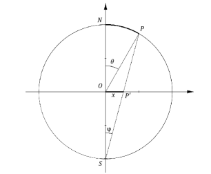
Figure 1. Stereographic coordinates

For $P^{\prime}$ we use cartesian coordinates $(x_{1},x_{2},...,x_{N},0)$. We also use $s=\sqrt{\sum_{i=1}^{N}x_{i}^{2}}$, the euclidean distance from $P^{\prime}$ to the origin $O$. As used we denote by $\theta$ the azimuthal angle, i. e. the angle between $ON$ and $OP$, where $N$ stands for the North Pole. Moreover we denote by $\varphi$ the angle between $SN$ and $SP$. It is clear that $\theta=2\varphi$ and $\tan\varphi=s$. Hence,

(8) $$\theta=2\arctan s$$

from which we immediately get

(9) $$\frac{d\theta}{ds}=\frac{2}{1+s^{2}}=p(s),$$

the conformal factor associated to the differential structure on $\mathbb{S}^{N}$. In terms of the conformal factor $p$ we can write

$$\nabla_{\mathbb{S}^{N}}=\frac{1}{p}\nabla_{\mathbb{R}^{N}},$$

where $\nabla_{\mathbb{R}^{N}}$ is the standard gradient on the equator. We also have

$$-\Delta_{\mathbb{S}^{N}}=-p^{-N}\mathrm{div}\left(p^{N-2}\nabla_{\mathbb{R}^{N}}u\right).$$

Finally, from the figure (or directly from (8) and (9)) we also have that

(10) $$\sin\theta=p\cdot s.$$

In the sequel we also need to compute $\theta_{,i}:=\dfrac{\partial\theta}{\partial x_{i}}$. Using (9), the definition of $s$ and the chain rule we have

$$\theta_{,i}=\frac{\partial\theta}{\partial s}\cdot s_{,i}=p\,\frac{x_{i}}{s},\quad i=1,...,N,$$

and

(11) $$\sum_{i=1}^{N}\theta_{,i}^{2}=p^{2}.$$

With the notation introduced above, we define

(12) $$\Phi_{i}(x)=G(\theta)\frac{x_{i}}{s},\quad i=1,...,N,$$

where $G(\theta)$ is defined in (7). In order to use $\Phi_{i}$ as test function in (3), we need the following orthogonality conditions

(13) $$\int_{\Omega}\Phi_{i}\,u_{j}\,d\omega=0,\quad i=1,...,N,\>j=0,...,i-1,$$

where, as we said, $u_{j}$ is an eigenfunction corresponding to $\mu_{j}(\Omega)$. To fulfill these conditions we need a special “orientation” of the sphere $\mathbb{S}^{N}$. When $j=0$, conditions (13) can be immediately deduced from Theorem 2.1 in [4] via the following identity

$$\int_{\Omega}\Phi_{i}\,d\omega=\int_{\Omega}G(\theta)\,\frac{x_{i}}{s}\,d\omega=\int_{\Omega}\frac{G(\theta)}{\sin\theta}\,y_{i}\,d\omega,$$

choosing $\tilde{G}(\theta)=\dfrac{G(\theta)}{\sin\theta}$. When $j>0$, conditions (13) can be proved arguing in an analogous way as in the proof of Theorem 2.1 in [3].

4. Proof of Theorem 1.1

Recalling the definition of $\Phi_{i}$ given in (12), we get

(14) $$\left(\nabla\Phi_{i}\right)_{j}\equiv\Phi_{i,j}=G^{\prime}(\theta)\,p\,\frac{x_{i}x_{j}}{s^{2}}+G(\theta)\,\frac{\delta_{ij}}{s}-G(\theta)\frac{x_{i}x_{j}}{s^{3}},\quad j=1,...,N.$$

Using (11), the definition of $s$ and (14) we have

(15) $$\frac{1}{p^{2}}\left|\nabla\Phi_{i}\right|^{2}=G^{\prime}(\theta)^{2}\frac{x_{i}}{s^{2}}+G(\theta)^{2}\frac{1}{s^{2}p^{2}}-G(\theta)^{2}\frac{x_{i}^{2}}{p^{2}s^{4}}.$$

Hence, from (10) and (15),

$$\sum_{i=1}^{N}\left|\left|\nabla_{\mathbb{S}^{N}}\Phi_{i}\right|\right|^{2}=\frac{1}{p^{2}}\sum_{i=1}^{N}\left|\nabla\Phi_{i}\right|^{2}=G^{\prime}(\theta)^{2}+G(\theta)^{2}\frac{N-1}{s^{2}p^{2}}=G^{\prime}(\theta)^{2}+G(\theta)^{2}\frac{N-1}{\sin^{2}\theta}.$$

Using $\Phi_{i}$ as test function in the variational characterization (3) of $\mu_{i}(\Omega)$, and taking into account the orthogonality conditions (13), we get

(16) $$\int_{\Omega}\Phi_{i}^{2}\,d\omega \leq \frac{1}{\mu_{i}(\Omega)}\int_{\Omega}G^{\prime}(\theta)^{2}\,\frac{x_{i}^{2}}{s^{2}}\,d\omega+\frac{1}{\mu_{i}(\Omega)}\int_{\Omega}\frac{G(\theta)^{2}}{\sin^{2}\theta}\left(1-\frac{x_{i}^{2}}{s^{2}}\right)\,d\omega$$

$$= \frac{1}{\mu_{i}(\Omega)}\int_{\Omega\cap D_{\gamma}}G^{\prime}(\theta)^{2}\,\frac{x_{i}^{2}}{s^{2}}\,d\omega+\frac{1}{\mu_{i}(\Omega)}\int_{\Omega}\frac{G(\theta)^{2}}{\sin^{2}\theta}\left(1-\frac{x_{i}^{2}}{s^{2}}\right)\,d\omega$$

$$\leq \frac{1}{\mu_{i}(\Omega)}\int_{D_{\gamma}}G^{\prime}(\theta)^{2}\,\frac{x_{i}^{2}}{s^{2}}\,d\omega+\frac{1}{\mu_{i}(\Omega)}\int_{\Omega}\frac{G(\theta)^{2}}{\sin^{2}\theta}\left(1-\frac{x_{i}^{2}}{s^{2}}\right)\,d\omega$$

$$= \frac{1}{N\,\mu_{i}(\Omega)}\int_{D_{\gamma}}G^{\prime}(\theta)^{2}\,d\omega+\frac{1}{\mu_{i}(\Omega)}\int_{\Omega}\frac{G(\theta)^{2}}{\sin^{2}\theta}\left(1-\frac{x_{i}^{2}}{s^{2}}\right)\,d\omega.$$

Summing over $i=1,...,N$ we get

$$\int_{\Omega}G(\theta)^{2}\,d\omega\leq\frac{1}{N}\sum_{i=1}^{N}\frac{1}{\mu_{i}(\Omega)}\int_{D_{\gamma}}G^{\prime}(\theta)^{2}\,d\omega+\sum_{i=1}^{N}\frac{1}{\mu_{i}(\Omega)}\int_{\Omega}\frac{G(\theta)^{2}}{\sin^{2}\theta}\left(1-\frac{x_{i}^{2}}{s^{2}}\right)\,d\omega.$$

Now notice that

$$\sum_{i=1}^{N}\frac{1}{\mu_{i}(\Omega)}\left(1-\frac{x_{i}^{2}}{s^{2}}\right)-\sum_{i=1}^{N-1}\frac{1}{\mu_{i}(\Omega)}=\frac{1}{\mu_{N}(\Omega)}-\sum_{i=1}^{N}\frac{1}{\mu_{i}(\Omega)}\,\frac{x_{i}^{2}}{s^{2}}\leq 0,$$

which follows from $\mu_{i}(\Omega)\leq\mu_{N}(\Omega)$ for all $i=1,...,N-1$ and the definition of $s$. Hence,

(17) $$\int_{\Omega}G(\theta)^{2}\,d\omega\leq\frac{1}{N}\sum_{i=1}^{N}\frac{1}{\mu_{i}(\Omega)}\int_{D_{\gamma}}G^{\prime}(\theta)^{2}\,d\omega+\sum_{i=1}^{N-1}\frac{1}{\mu_{i}(\Omega)}\int_{\Omega}\frac{G(\theta)^{2}}{\sin^{2}\theta}\,d\omega.$$

By Lemma 2.1 we know that the function $\dfrac{G(\theta)}{\sin\theta}$ is decreasing in $(0,\gamma)$. Recalling that $|\Omega|=|D_{\gamma}|$, we get

(18) $$\int_{\Omega}\frac{G(\theta)^{2}}{\sin^{2}\theta}\,d\omega = \int_{\Omega\cap D_{\gamma}}\frac{G(\theta)^{2}}{\sin^{2}\theta}\,d\omega+\int_{\Omega\setminus D_{\gamma}}\frac{G(\theta)^{2}}{\sin^{2}\theta}\,d\omega$$

$$\leq \int_{\Omega\cap D_{\gamma}}\frac{G(\theta)^{2}}{\sin^{2}\theta}\,d\omega+\frac{G(\gamma)^{2}}{\sin^{2}\gamma}\,|\Omega\setminus D_{\gamma}|$$

$$= \int_{\Omega\cap D_{\gamma}}\frac{G(\theta)^{2}}{\sin^{2}\theta}\,d\omega+\frac{G(\gamma)^{2}}{\sin^{2}\gamma}\,|D_{\gamma}\setminus\Omega|$$

$$\leq \int_{\Omega\cap D_{\gamma}}\frac{G(\theta)^{2}}{\sin^{2}\theta}\,d\omega+\int_{D_{\gamma}\setminus\Omega}\frac{G(\theta)^{2}}{\sin^{2}\theta}\,d\omega$$

$$= \int_{D_{\gamma}}\frac{g(\theta)^{2}}{\sin^{2}\theta}\,d\omega.$$

On the other side, since $G(\theta)$ is non-decreasing in $\left(0,\frac{\pi}{2}\right)$, we have

(19) $$\int_{\Omega}G(\theta)^{2}\,d\omega = \int_{\Omega\cap D_{\gamma}}G(\theta)^{2}\,d\omega+\int_{\Omega\setminus D_{\gamma}}G(\theta)^{2}\,d\omega$$

$$\geq \int_{\Omega\cap D_{\gamma}}G(\theta)^{2}\,d\omega+G(\gamma)^{2}|\Omega\setminus D_{\gamma}|$$

$$= \int_{\Omega\cap D_{\gamma}}G(\theta)^{2}\,d\omega+G(\gamma)^{2}|D_{\gamma}\setminus\Omega|$$

$$\geq \int_{\Omega\cap D_{\gamma}}G(\theta)^{2}\,d\omega+\int_{D_{\gamma}\setminus\Omega}g(\theta)^{2}\,d\omega$$

$$= \int_{D_{\gamma}}g(\theta)^{2}\,d\omega.$$

Using (17), (18), (19) and the monotonicity of the sequence $\{\mu_{i}(\Omega)\}_{i}$ we have

$$\int_{D_{\gamma}}g(\theta)^{2}\,d\omega \leq \frac{1}{N}\sum_{i=1}^{N}\frac{1}{\mu_{i}(\Omega)}\int_{D_{\gamma}}g^{\prime}(\theta)^{2}\,d\omega+\sum_{i=1}^{N-1}\frac{1}{\mu_{i}(\Omega)}\int_{D_{\gamma}}\frac{g(\theta)^{2}}{\sin^{2}\theta}\,d\omega$$

$$\leq \frac{1}{N-1}\sum_{i=1}^{N-1}\frac{1}{\mu_{i}(\Omega)}\int_{D_{\gamma}}\left[g^{\prime}(\theta)^{2}+(N-1)\,\frac{g(\theta)^{2}}{\sin^{2}\theta}\right]\,d\omega.$$

Finally, from (6) we conclude

(20) $$\frac{1}{N-1}\sum_{i=1}^{N-1}\frac{1}{\mu_{i}(\Omega)}\geq\frac{1}{\mu_{1}(D_{\gamma})}.$$

The equality sign holds in (20) if and only if $\Omega$ is a geodesic ball.

References

- [1] M. S. Ashbaugh, Open problems on eigenvalues of the Laplacian, Analytic and geometric inequalities and applications, 13–28, Math. Appl., 478, Kluwer Acad. Publ., Dordrecht, 1999.
- [2] M. S. Ashbaugh, and R. D. Benguria, A sharp bound for the ratio of the first two eigenvalues of Dirichlet Laplacians and extensions, Ann. of Math. (2) 135 (1992), no. 3, 601–628.
- [3] M. S. Ashbaugh, and R. D. Benguria, Universal bounds for the low eigenvalues of Neumann Laplacians in dimensions, SIAM J. Math. Anal. (24) 3 (1993), 557–570.
- [4] M. S. Ashbaugh, and R. D. Benguria, Sharp upper bound to the first nonzero Neumann eigenvalue for bounded domains in spaces of constant curvature, J. London Math. Soc. (2) 52 (1995), 402–416.
- [5] M. S. Ashbaugh, and R. D. Benguria, A sharp bound for the ratio of the first two Dirichlet eigenvalues of a domain in a hemisphere of , Trans. Amer. Math. Soc. 353 (2001), no. 3, 105–1087.
- [6] C. Bandle, Isoperimetric inequalities and applications, Monographs and Studies in Mathematics, 7. Pitman , Boston, Mass.-London, 1980.
- [7] F. Brock, and F. Chiacchio, in preparation.
- [8] F. Brock, F. Chiacchio, and G. di Blasio, Optimal Szegö-Weinberger type inequalities, Commun. Pure Appl. Anal. 15 (2016), no. 2, 367–383.
- [9] D. Bucur, and A. Henrot, Maximization of the second non-trivial Neumann eigenvalue, aeXiv:1801.07435v1.
- [10] I. Chavel, Eigenvalues in Riemannian geometry, Academic, New York, 1984.
- [11] I. Chavel, Lowest-eigenvalue inequalities, in: Geometry of the Laplace Operator, Proc. Sympos. Pure Math., Univ. Hawaii, Honolulu, Hawaii (1979), in: Proc. Sympos. Pure Math., vol. XXXVI, American Mathematical Society, Providence, RI, 1980, 79–89.
- [12] F. Chiacchio, and G. di Blasio, Isoperimetric inequalities for the first Neumann eigenvalue in Gauss space, Ann. Inst. H. Poincaré Anal. Non Linéaire 29 (2012), no. 2, 199–216.
- [13] L. Grafakos, Modern Fourier analysis. Third edition. Graduate Texts in Mathematics, 250. Springer, New York, 2014.
- [14] A. Henrot, Extremum problems for eigenvalues of elliptic operators. Frontiers in Mathematics. Birkhäuser Verlag, Basel, 2006.
- [15] A. Henrot (ed), Shape Optimization and Spectral Theory. De Gruyter open (2017), freely downloadable at https://www.degruyter.com/view/product/490255.
- [16] R.S. Laugesen, and B. A. Siudeja, Maximizing Neumann fundamental tones of triangles, J. Math. Phys. 50 (2009), no. 11, 112903, 18 pp.
- [17] G. Szegő, Inequalities for certain eigenvalues of a membrane of given area, J. Rational Mech. Anal. 3, (1954), 343–356.
- [18] Q. Wang, and C. Xia, On a conjecture of Ashbaugh and Benguria about lower eigenvalues of the Neumann Laplacian, arXiv:1808.09520v1.
- [19] H. Weinberger, An isoperimetric inequality for the -dimensional free membrane problem, J. Rational Mech. Anal. 5 (1956), 633–636.