Odd-Frequency Pairs in Chiral Symmetric Systems:
Spectral Bulk-Boundary Correspondence and Topological Criticality

Abstract

Odd-frequency Cooper pairs with chiral symmetry emerging at the edges of topological superconductors are a useful physical quantity for characterizing the topological properties of these materials. In this work, we show that the odd-frequency Cooper pair amplitudes can be expressed by a winding number extended to a nonzero frequency, which is called a “spectral bulk-boundary correspondence,” and can be evaluated from the spectral features of the bulk. The odd-frequency Cooper pair amplitudes are classified into two categories: the amplitudes in the first category have the singular functional form $\sim 1/z$ (where $z$ is a complex frequency) that reflects the presence of a topological surface Andreev bound state, whereas the amplitudes in the second category have the regular form $\sim z$ and are regarded as non-topological. We discuss the topological phase transition by using the coefficient in the latter category, which undergoes a power-law divergence at the topological phase transition point and is used to indicate the distance to the critical point. These concepts are established based on several concrete models, including a Rashba nanowire system that is promising for realizing Majorana fermions.

Introduction.— The findings of quantum Hall systems and topological insulators have introduced topology into condensed matter physics PG (8); G.R.Volovik (2003); Hasan and Kane (2010), leading to the discovery of a host of topological materials. One important property of topological systems is that the number of edge modes including the zero energy state is predicted by the topological number, which is defined by the bulk Ryu and Hatsugai (2002); Ryu et al. (2010); Qi and Zhang (2011); Sato and Fujimoto (2016); Chiu et al. (2016); Sato and Ando (2017); Rhim et al. (2018). This relation is called the “bulk-boundary correspondence” and has been a key concept in condensed matter physics Hatsugai (1993a); Schnyder et al. (2008).

The surface Andreev bound states (SABSs) in topological superconductors are associated with a nontrivial topological number, and some are Majorana fermions Sato et al. (2011a); Tanaka et al. (2012). In terms of Cooper pairs, the SABSs indicate the presence of odd-frequency Cooper pairs at the boundary, which have an odd functional form in time and frequency Tanaka et al. (2007a, b, 2012). Such exotic Cooper pairing was first proposed by Berezinskii Berezinskii (1974), and the corresponding realization was discussed not only in the bulk state Kirkpatrick and Belitz (1991); Balatsky and Abrahams (1992); Emery and Kivelson (1992); Coleman et al. (1997) but also in a number of systems such as superconducting junctions based on ferromagnets Bergeret et al. (2001); Eschrig et al. (2003); Eschrig (2015), diffusive normal metals Tanaka and Golubov (2007), and vortex cores Yokoyama et al. (2008); Tanuma et al. (2009). In addition, their peculiar paramagnetic responses have also been discussed Yokoyama et al. (2011); Suzuki and Asano (2014, 2015); Lee et al. (2017); Di Bernardo et al. (2015), and the odd-frequency pairing has become a topic of interest in condensed matter physics Tanaka et al. (2012); Linder and Balatsky (2017); Fleckenstein et al. (2018). For SABSs in topological superconductors, the relevance of the odd-frequency pairing is known Asano and Tanaka (2013); Stanev and Galitski (2014); Liu et al. (2015); Ebisu et al. (2016); Crépin et al. (2015); Cayao and Black-Schaffer (2017); Keidel et al. (2018); Fleckenstein et al. (2018); Cayao and Black-Schaffer (2018); the pair amplitude has a singular functional form and diverges at zero frequency, $F^{\rm odd}_{\rm edge}(z)\sim 1/z$, with complex frequency $z$. This formula is distinct from the regular form [$F^{\rm odd}_{\rm edge}(z)\sim z$], which appears ubiquitously because of the broken symmetry (e.g., the absence of translational symmetry at the edge) Tanaka et al. (2007a, b); Eschrig et al. (2007). Thus, the topological superconducting systems offer a unique testing ground to develop ways to control the properties of odd-frequency Cooper pairing and to improve our understanding of Cooper pairs.

The search for topological superconductivity has led to intensive studies of the chiral symmetric systems Sato et al. (2011a); Tanaka et al. (2010); Yada et al. (2011); Heikkilä et al. (2011); Brydon et al. (2011); Schnyder et al. (2012); Tewari and Sau (2012); Wong and Law (2012), including Rashba nanowire systems, which are promising for experimental realization of Majorana fermions at the edge Lutchyn et al. (2010); Oreg et al. (2010) and expected for a platform of a topological quantum computing Kitaev (2001); Bravyi and Kitaev (2002); Sarma et al. (2015). The chiral operator $\Gamma$ anticommutes with the Hamiltonian ($\{\Gamma,{\cal H}\}=0$). The index theorem tells us that the winding number defined in the bulk predicts the number of SABSs via the bulk-boundary correspondence Sato et al. (2011a). The chiral symmetric systems also include a non-superconducting topological insulator such as a Su-Schrieffer-Heeger (SSH) model Su et al. (1979); Heeger et al. (1988) and Shockley model Shockley (1939); Pershoguba and Yakovenko (2012).

In this Letter, we extend the bulk-boundary correspondence from zero frequency to nonzero frequency, which we call “spectral bulk-boundary correspondence” (SBBC). By using the SBBC, the odd-frequency Cooper pairs accumulated at the boundary can be evaluated from the physical quantity determined in the bulk over the entire frequency range. We further clarify that the regular odd-frequency Cooper pair amplitude ($\sim z$) can be used as a degree of proximity to the topological phase transition, which is analogous to using the susceptibility as a degree of the proximity to the phase transition in standard statistical physics. The coefficient follows a power-law divergence at the topological phase transition, which reveals the topological criticality. Thus, we identify the fluctuation behavior associated with the topological transition, and can even go beyond the simple integer classification of phases.

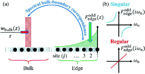
Figure 1: (a) Schematic of the correspondence between odd-frequency Cooper pair correlation $F_{\mathrm{edge}}^{\mathrm{odd}}(z)$ and the extended winding number $w_{\mathrm{bulk}}(z)$ with complex frequency $z$. (b) Graphs of singular and regular frequency dependence of $F_{\mathrm{edge}}^{\mathrm{odd}}$. $z=i\omega_{n}$ is a Matsubara frequency and if $z$ is purely imaginary, $F_{\mathrm{edge}}^{\mathrm{odd}}$ is also purely imaginary.

SBBC.— We begin by demonstrating the SBBC. The following relation holds for chiral symmetric systems and for any complex frequency $z\in\mathbb{C}$:

$$F_{\mathrm{edge}}^{\mathrm{odd}}(z)= \frac{w_{\mathrm{bulk}}(z)}{z},$$ (1)

with

$$F_{\mathrm{edge}}^{\mathrm{odd}}(z)= \underset{j}{\mathrm{Tr}}\left[\Gamma G(z)\right],$$ (2)

$$w_{\mathrm{bulk}}(z)= \tfrac{{\rm i}}{2}\underset{k}{\mathrm{Tr}}\left[\Gamma G(z)\partial_{k}G^{-1}(z)\right]$$ (3)

where the trace in Eq. (2) is taken over a semi-infinite space: ${\rm Tr}_{j}\cdots={\rm tr}\sum_{j=1}^{\infty}\langle j|\cdots|j\rangle$. The surface is located on the right side, as shown in Fig. 1(a), and the site index is a positive integer. The Green’s function is defined by $G(z)=1/(z-{\cal H})$ with the Hamiltonian $\mathcal{H}$. The trace ${\rm tr}$ is taken over the internal degrees of freedom composed of, e.g., spin and orbital indices. On the other hand, the trace $\mathrm{Tr}_{k}$ in Eq. (3) is taken over the bulk labeled by the wave vectors: ${\rm Tr}_{k}\cdots={\rm tr}\int_{-\pi}^{\pi}\frac{dk}{2\pi}\langle k|\cdots|k\rangle$. A schematic of $F_{\mathrm{edge}}^{\mathrm{odd}}(z)$ and $w_{\mathrm{bulk}}(z)$ appears in Fig. 1(a).

In the zero-frequency limit, $w_{\rm bulk}(z\rightarrow 0)\equiv W$ is identified as the winding number Gurarie (2011). The full profile of $w_{\rm bulk}(z)$ is then regarded as an extension of the winding number to nonzero frequency. The quantity $F^{\rm odd}_{\rm edge}(z)$ is the off-diagonal component of the Green’s function located at the edge and represents the pair amplitude for topological superconductors. We confirm that both sides of Eq. (1) are odd in $z$, meaning that $F^{\rm odd}_{\rm edge}(z)$ relevant to the SBBC is an odd-frequency Cooper pair amplitude. At zero frequency, Eq. (1) connects the nontrivial topological number $W\neq 0$ to the odd-frequency pair through the singular functional form $F^{\rm odd}_{\rm edge}(z\rightarrow 0)=W/z$ [Fig. 1(b)]. Furthermore, Eq. (1) shows that this connection persists to finite frequencies, which extends the concept of conventional frequency-independent bulk-boundary correspondence Hatsugai (1993b). This means that the total amount of the odd frequency Cooper pair correlation accumulated near the surface is predicted by the bulk value [$w_{\mathrm{bulk}}(z)/z$].

Equation (1) is confirmed exactly in various limits of a Kitaev chain Kitaev (2001), and is also confirmed numerically for various chiral symmetric systems such as Rashba nanowires Lutchyn et al. (2010); Oreg et al. (2010), and two-dimensional $d_{x^{2}-y^{2}}$-wave superconductors Yada et al. (2011); Kashiwaya and Tanaka (2000). We first take a closer look at the SBBC in the Kitaev chain which is a one-dimensional $p$-wave superconductor with fully polarized spins [see Fig. 2(a)]. The Hamiltonian is ${\cal H}=\sum_{k}C_{k}^{\dagger}H(k)C_{k}$ with

$$H(k)= -(t\cos k+\mu/2)\tau_{3}-\Delta\sin k\tau_{2}$$ (4)

and $C_{k}={(c_{k},c_{-k}^{\dagger})}^{\mathrm{T}}$ where $c_{k}$ is an annihilation operator of electrons. $t$ is a hopping integral and $\mu$ is a chemical potential, $\tau_{\mu}$ ($\mu=1,2,3$) is a Pauli matrix in Nambu space, and $\Delta$ is the $p$-wave superconducting gap. The condition for a topological superconductor is $|\mu|<\mu_{\mathrm{c}}=2t$. We now show that $F_{\mathrm{edge}}^{\mathrm{odd}}(z)$ corresponds to the odd-frequency Cooper pair amplitude. We first set $z=i\omega_{n}$, where $\omega_{n}$ is an imaginary (Matsubara) frequency. The chiral operator $\Gamma$ for a semi-infinite system is $\Gamma=\mathrm{diag}(\ldots,\tau_{1},\tau_{1}),$ where $\tau_{1}$ is a Pauli matrix acting on a Nambu space $(c_{j},\ c_{j}^{\dagger})$. The function $F_{\rm edge}^{\rm odd}(z)$ is then

$$F_{\rm edge}^{\rm odd}({\rm i}\omega_{n})= \int_{0}^{\mathrm{\beta}}\mathrm{d}\tau e^{\mathrm{i}\omega_{n}\tau}\sum_{j=1}^{\infty}\langle c_{j}(\tau)c_{j}(0)\rangle+{\rm c.c.},$$ (5)

where the right-hand side is the Cooper pair amplitude for $s$-wave spin-triplet superconductivity and must be an odd function in time and frequency to satisfy the Pauli exclusion principle.

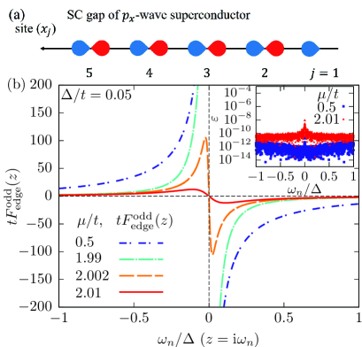
Figure 2: (a) Schematic of one-dimensional $p$-wave pairing Kitaev chain. (b) The imaginary part of total amount of the odd frequency Cooper pair amplitude $\mathrm{Im}[F_{\mathrm{edge}}^{\mathrm{odd}}(z)]$ is plotted as a function of $\omega_{n}=z/i$ at $\Delta/t=0.05$ with several $\mu$. In the inset, $\varepsilon$ is plotted as a function of $\omega_{n}$ for $\mu/t=0.5$ and 2.01.

When the special conditions $t=\Delta$ and $\mu=0$ are satisfied, Majorana fermions are localized at the edges of the system with zero localization length. In this case, the SBBC relation (1) takes the analytical form

$$F_{\mathrm{edge}}^{\mathrm{odd}}(z)= \frac{w_{\mathrm{bulk}}(z)}{z}=\frac{-t^{2}}{z(z^{2}-t^{2})}.$$ (6)

See the supplementary material (SM) for more a detailed derivation [SM from I-A to I-E]. We can also construct the quasi-classical Green’s function for a coherence length sufficiently large compared with the inverse Fermi momentum. The SBBC also takes the following analytical form in this limit [SM I-F]:

$$F_{\mathrm{edge}}^{\mathrm{odd}}(z)= \frac{w_{\mathrm{bulk}}(z)}{z}=\frac{\Delta}{z\sqrt{\Delta^{2}-z^{2}}}.$$ (7)

In Eq. (7), we assume $\mu\gg|z|$ and $\mu\gg\Delta$ where we measure the chemical potential from the bottom of the band. Let us also consider the numerical results for the Kitaev chain with $\Delta/t=0.05$ and $\mu\neq 0$. Figure 2(b) plots $F_{\mathrm{edge}}^{\mathrm{odd}}(z)$ as a function of $\omega_{n}$ for several $\mu/t$. The parameters $\mu/t=0.5$ and $1.998$ are located in the topological region: in the limit $\omega_{n}\rightarrow 0$, it diverges as $\omega_{n}$ approaches zero (singular). For $\mu/t=2.002$ and 2.01, however, it approaches zero for $\omega_{n}\rightarrow 0$ (regular). To check the numerical accuracy of the SBBC we calculate the quantity $\varepsilon(z)=|{F}_{\mathrm{edge}}^{\mathrm{odd}}(z)-{w}_{\mathrm{bulk}}(z)/z|/{|{w}_{\mathrm{bulk}}(z)/z|}$, which is less than $10^{-10}$ for $\mu/t=0.5$ and 1.998 (i.e., the same within numerical error). For $\mu/t=2.002$ and 2.01, $\varepsilon<10^{-8}$ [SM I-G]. We also checked the SBBC for spatially changing pair potentials near the edge, which are discussed in detail in the SM I-H.

Topological criticality in odd-frequency Cooper pairs.— The topological criticality has been discussed in terms of the physical quantities such as divergent correlation length, compressibility Mondragon-Shem et al. (2014); Altland et al. (2014); Seo et al. (2013, 2013); Chan et al. (2015); Tewari et al. (2012); Serina et al. (2018). Here we demonstrate that the criticality appears also in the odd-frequency Cooper pairs. In the low-frequency limit, the odd frequency Cooper pair amplitude is

$$F_{\rm edge}^{\rm odd}(z) =\frac{W}{z}+\chi z+O(z^{3}).$$ (8)

The first term on the right-hand side represents the singular odd-frequency pair, and the second term represents the regular pair. The quantity $W=w_{\rm bulk}(z=0)$ is a standard winding number defined in the bulk. By using the SBBC, $\chi$ can be expressed as a bulk quantity: $\chi=\tfrac{{\rm i}}{2}{\rm Tr}_{k}\left[\Gamma H^{-3}\partial_{k}H\right]$. We find that at the topological quantum phase transition where $W$ changes, the coefficient $\chi$ undergoes a power law divergence upon approaching from either side of the phases. As shown in Fig. 3(b), the critical behavior in the limit $\mu\to\mu_{\mathrm{c}}$ is $\chi\sim|\mu-\mu_{\mathrm{c}}|^{-2}$. However, this exponent crossovers into another ones, namely $-1$ for $\mu<\mu_{\mathrm{c}}$ and $-5/2$ for $\mu>\mu_{\mathrm{c}}$ [SM I-I], and thus the behavior is quite asymmetric around the critical point $\mu=\mu_{\mathrm{c}}$ as in Fig. 3(a). While the exponent $-2$ is consistent with the Ising universality Sachdev (2011), for the exponents $-1$ and $-5/2$, one needs a generalization of the concept.

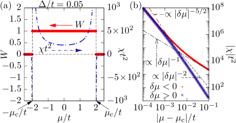
Figure 3: (a) The winding number $W$ (left vertical axis) and $\chi$ (right vertical axis) are plotted as a function of $\mu$ for $\Delta/t=0.05$. (b) $|\chi|$ is plotted near $\mu_{\mathrm{c}}$ as a function of $|\mu-\mu_{\mathrm{c}}|/t$ for $\mu>\mu_{\mathrm{c}}$ and $\mu<\mu_{\mathrm{c}}$ with $\mu_{\mathrm{c}}=2t$ and $\delta\mu=\mu-\mu_{\mathrm{c}}$.

In order to understand the above critical behaviors, we use scaling theory for the effective action. The effective low-energy action is introduced as

$$S=\int\mathrm{d}\tau\mathrm{d}x\Big{[}\psi^{\dagger}\partial_{\tau}\psi+\frac{v}{2}\left(\psi^{\dagger}\partial_{x}\psi^{\dagger}+{\rm H.c.}\right)+m\psi^{\dagger}\psi-\Lambda\psi^{\dagger}\partial_{x}^{2}\psi\Big{]},$$ (9)

where $v$ is a velocity, $m$ is a mass and $\Lambda$ is a coefficient of the second derivative term. For the Kitaev chain, $v$, $m$ and $\Lambda$ are given by $v=\Delta$, $m=\delta\mu=\mu-\mu_{\mathrm{c}}$ and $\Lambda=t$, respectively. The corresponding energy is given by $\lambda_{k}^{2}={(m+\Lambda k^{2})}^{2}+v^{2}k^{2}$. Usually the term with $\Lambda$ is irrelevant and can be neglected and one obtains the Ising universality. However, in superconductors $v=\Delta$ is an energy gap and hence not only $m$ (distance to critical point) but also $v$ are much smaller than $\Lambda$. In this case, the quadratic term must be kept, to result in a variety of critical behaviors (see Fig. 3). We perform the scale transformation as $x^{\prime}=xe^{-l}$ ($\dim[x]=-1$). The action in the low-temperature limit is invariant if the scaling dimensions satisfy $\dim[\psi]=1/2$, $\dim[\tau]=-2$ (dynamical critical exponent), $\dim[v]=1$, and $\dim[m]=2$.

Now let us consider the generalized winding number in the expansion form $w_{\mathrm{bulk}}(z)=\sum_{n=0}^{\infty}a_{2n}z^{2n}$ (specifically, $a_{0}=W$ and $a_{2}=\chi$). In the critical region $|\Lambda|\gg|m|,|v|$, we can express the coefficients as $a_{2n}(m,v)=a^{\prime}_{2n}v^{\alpha_{n}}m^{\beta_{n}}$. Using the fact that the scaling dimension of $w_{\mathrm{bulk}}(z)$ is zero, we have the relation between $\alpha_{n}$ and $\beta_{n}$:

$$\alpha_{n}\dim[v]+\beta_{n}\dim[m]+2n\dim[z]=0.$$ (10)

The odd-frequency pair amplitude can now be written as

$$F^{\mathrm{odd}}_{\mathrm{edge}}(z)=\frac{1}{z}\mathcal{W}\left(\frac{v}{\sqrt{\Lambda m}},\frac{z^{2}}{m^{2}}\right),$$ (11)

by using the SBBC. Namely, the odd-frequency pair amplitude is generally a function of three independent variables ($z,m,v$ with $\Lambda$ being unit of energy), but for $|m|,|v|\ll|\Lambda|$ they are reduced to two variables. From the shapes of the energy spectrum shown in Fig. 4, we can identify the three regimes, in which $F^{\mathrm{odd}}_{\mathrm{edge}}(z)$ can be written by a single scaling function with only one variable. Correspondingly we obtain three quantum critical regions (QCR) QCR1, QCR2 and QCR3 shown in Fig. 4 [detailed derivation is shown in SM I-J], which gives exponents $\chi$ behaving as $v^{0}m^{-2}$ in QCR1, $v^{-2}m^{-1}$ in QCR2 and $v^{1}m^{-5/2}$ in QCR3. These critical exponents can also seen in Fig. 3(b)

Our results thus extend the conventional knowledge about topological phase transitions. Since the low-energy effective actions for Rashba nanowire and $d$-wave superconductors are given by the same action as that in the Kitaev chain, we get the similar critical behaviors as demonstrated in the following.

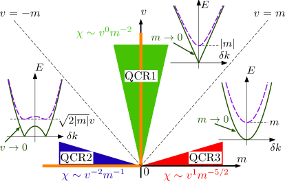
Figure 4: Critical regimes for the Kitaev chain near $\mu=\mu_{\mathrm{c}}$ and $\Delta=0$, illustrated in the plane of the mass $m(\propto\mu-\mu_{c})$ and velocity $v(\propto\Delta)$. Colored regions (QCR1 to QCR3) are characterized by different critical exponents $\chi\sim v^{\alpha}m^{\beta}$ with fixed $\alpha+2\beta=-4$. The orange line shows the critical points at which the energy gap closes.

Rashba nanowire.— The SBBC and singular behavior of the regular odd-frequency pair amplitude can also be seen in the other models; e.g., the one-dimensional Rashba nanowire on an $s$-wave superconductor Lutchyn et al. (2010); Oreg et al. (2010), where a Majorana fermion located at the edge is accompanied by odd-frequency pairing Asano and Tanaka (2013); Stanev and Galitski (2014) [see Fig. 5(a)]. The Hamiltonian is given by ${\cal H}=\frac{1}{2}\sum_{k}C_{k}^{\dagger}H(k)C_{k},$ with

$$H(k)= \left[\varepsilon(k)\sigma_{0}+V_{\mathrm{ex}}\sigma_{3}+\lambda\sin k\sigma_{2}\right]\tau_{3}+\Delta\mathrm{i}\sigma_{2}\mathrm{i}\tau_{2},$$ (12)

where $C_{k}={\left(c_{k,\uparrow},c_{k,\downarrow},c_{-k,\uparrow}^{\dagger},c_{-k,\downarrow}^{\dagger}\right)}^{\rm T}$ , $\varepsilon(k)=-2t\cos(k)+2t-\mu$, $V_{\mathrm{ex}}$ is a magnetic field, $\lambda$ is the Rashba spin orbit interaction, and $\Delta$ is an $s$-wave superconducting gap. $\sigma_{\mu}$ ($\mu=1,2,3$) is a Pauli matrix in spin space. The system is located in the topological regime when $\sqrt{\mu^{2}+\Delta^{2}}<|V_{\mathrm{ex}}|<\sqrt{{(4t-\mu)}^{2}+\Delta^{2}}$. The chiral operator can be defined provided the magnetic field and the spin-orbit interaction are orthogonal: $\Gamma=\sigma_{0}\tau_{1}$. The energy dispersion of the Rashba nanowire is shown in Fig. 5(b).

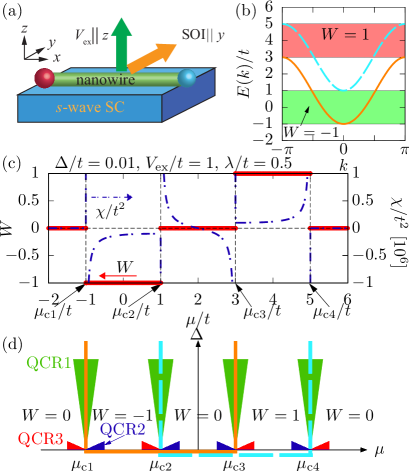
Figure 5: (a) Schematic of Rashba nanowire. (b) Energy dispersion of nanowire for $\Delta/t=0.01$, $V_{\mathrm{ex}}/t=1$, $\lambda/t=0.5$, and $\mu=0$. The red and green shaded areas are the topological regime. (c) $W$ (red, left vertical axis) and $\chi$ (blue, right vertical axis) are plotted as a function of $\mu/t$. $\mu_{c1}=-\sqrt{V_{\mathrm{ex}}^{2}-\Delta^{2}}$, $\mu_{c2}=\sqrt{V_{\mathrm{ex}}^{2}-\Delta^{2}}$, $\mu_{c3}=4t-\sqrt{V_{\mathrm{ex}}^{2}-\Delta^{2}}$, and $\mu_{c4}=4t+\sqrt{V_{\mathrm{ex}}^{2}-\Delta^{2}}$. (d) Schematic of the QCRs. 

We discuss criticality for Rashba nanowire. Figure 5(c) shows $W$ and $\chi$ as a function of $\mu$. The parameter $\chi$ diverges near the quantum transition points, showing topological criticality. A very sharp divergence appears when e.g., $\mu\rightarrow-\sqrt{V_{\mathrm{ex}}^{2}-\Delta^{2}}-0$, which is due to the small magnitude of the superconducting gap (see also the SM II-A and II-B).

The criticality of the Rashba nanowire is understood by using the results for the Kitaev chain as a building block. The energy dispersion in Fig. 5(b) is viewed as two coupled nanowires; there are two cosine-like dispersions and they are regarded as double Kitaev chain. $\mu_{c1}$ ($\mu_{c2}$) and $\mu_{c3}$ ($\mu_{c4}$) are the lower and upper boundary of the energy dispersion shown by orange line (light blue dotted line). The orange and light blue lines in Fig. 5(d) correspond to the band edges at which energy gap closes (i.e., at critical point). For small $\Delta$ ($\ll t$), which is usually satisfied in superconductors, the phase diagram in Fig. 4 can be applied for each band edge. Then QCR2 with $\chi\sim{(\mu-\mu_{\mathrm{c}})}^{-1}$ [QCR3 with $\chi\sim{(\mu-\mu_{\mathrm{c}})}^{-5/2}$] exists inside (outside) of each energy dispersion as shown in Fig. 5(d). Thus complex and highly asymmetric behaviors of $\chi$ around topological transition are explained based on Fig. 4. Note that the sign of $\chi$ changes at $\mu/t=2$ in the non-topological regime. This property reflects the situation in which this non-topological phase is sandwiched between topological phases with the different winding numbers $W=+1$ and $W=-1$. Namely, we can obtain information on the neighboring topological phases even in the non-topological phase by looking at the regular odd-frequency Cooper pairs. In contrast, no such sign change appears for the Kitaev chain.

$d$-wave superconductors.— We also calculate $W$ and $\chi$ for $d_{x^{2}-y^{2}}$-wave superconductor with (11)-surface [shown in SM III-A]. In this case, $W$ changes its value as a function of a wave number which is parallel to the surface and $\chi$ also diverges at topological transition points [SM III-B].

Conclusion.— We demonstrate that the SBBC $F_{\mathrm{edge}}^{\mathrm{odd}}(z)=w_{\mathrm{bulk}}(z)/z$ [Eq. (1)] holds for chiral symmetric systems such as the Kitaev chain, Rashba nanowire which is promising for the realization of the Majorana fermion, and two dimensional $d_{x^{2}-y^{2}}$-wave superconductors. The Cooper pair amplitude can be expanded to the form $F_{\mathrm{edge}}^{\mathrm{odd}}(z)=W/z+\chi z+\mathcal{O}(z^{3})$, where $W$ is a topological number. We show that the coefficient $\chi$ diverges at the topological transition point and the critical behaviors are interpreted in terms of the effective action which generalizes the known Ising universality class.

Note added.— After submission of our previous version [arXiv:1809.05687v1 (2018)], we are aware that Daido and Yanase have submitted a proof of the SBBC based on a chirality polarization [arXiv:1901.03482v1 (2019)].

Supplemental Material for
“Odd-frequency pairs in chiral symmetric systems: spectral bulk-boundary correspondence and topological criticality”

I Kitaev chain

In I.1, a Hamiltonian for the Kitaev chain and a formal formula of $w_{\mathrm{bulk}}(z)$ are introduced. Next four subsections are analytical results for $t=\Delta$. In I.2, an analytical formula for $w_{\mathrm{bulk}}(z)$ with $t=\Delta$ is given. In I.3, we explain the derivation of a surface Green’s function for the Kitaev chain and in I.4, we give a local Green’s function for arbitrary site. In I.5, the local Green’s function for $\mu=0$ is given and the spectral bulk-boundary correspondence (SBBC) is analytically shown. In I.6, we show the SBBC holds for the continuum model of the $p$-wave superconductor. Following two subsections are numerical results for $F_{\mathrm{edge}}^{\mathrm{odd}}(z)$ and $w_{\mathrm{bulk}}(z)/z$. In I.7, we numerically calculate $F_{\mathrm{edge}}^{\mathrm{odd}}(z)$ and $w_{\mathrm{bulk}}(z)/z$ for $\Delta/t=1$ and $\Delta/t=0.05$, and in I.8, we introduce spatial modulation near the surface of the gap function and the chemical potential. We give an exact formula of $\chi$ for Kitaev chain with arbitrary $\Delta$ in I.9. Finally, we explain the critical exponent of $\chi$ in I.10.

I.1 Hamiltonians with open boundary and periodic boundary condition

The Kitaev chain in the real-space basis is

$${\cal H}= -t\sum_{j}\left(c_{j}^{\dagger}c_{j+1}+\mathrm{H.c.}\right)+\Delta\sum_{j}\left(c_{j+1}^{\dagger}c_{j}^{\dagger}+\mathrm{H.c.}\right)$$

$$-\mu\sum_{j}c_{j}^{\dagger}c_{j},$$ (S1)

where $c_{j}$ is an annihilation operator on $j$-th site and $t$ is the hopping integral, $\Delta$ is the $p$-wave superconducting gap and $\mu$ is the chemical potential.

For the open boundary (OB) condition with $n$-site system, the Hamiltonian is

$${\cal H}^{\mathrm{OB}}_{n}= C_{n}^{\dagger}\begin{pmatrix}\hat{u}&\hat{t}\\ \hat{t}^{\dagger}&\hat{u}&\hat{t}\\ &\hat{t}^{\dagger}&\hat{u}&\ddots\\ &&\ddots&\ddots&\end{pmatrix}C_{n},$$ (S2)

$$C_{n}= \left(c_{n},\>c_{n}^{\dagger},\>c_{n-1},\>c_{n-1}^{\dagger},\>\ldots,c_{1},\>c_{1}^{\dagger}\right)^{\mathrm{T}},$$ (S3)

$$\hat{u}= \frac{1}{2}\begin{pmatrix}-\mu&0\\ 0&\mu\end{pmatrix},$$ (S4)

$$\hat{t}= \frac{1}{2}\begin{pmatrix}-t&\Delta\\ -\Delta&t\end{pmatrix}.$$ (S5)

We define a Green’s function corresponding to ${\cal H}_{n}^{\mathrm{OB}}$ as

$$G_{n}(z)= \frac{1}{z-{\cal H}_{n}^{\mathrm{OB}}}.$$ (S6)

On the other hand, by imposing the periodic boundary condition on Eq. (S1), we obtain the Hamiltonian with the wave number basis as

$${\cal H}_{\mathrm{bulk}}= \sum_{k}C_{k}^{\dagger}H_{\mathrm{bulk}}(k)C_{k},$$ (S7)

$$C_{k}= \left(c_{k},\>c_{-k}^{\dagger}\right)^{\mathrm{T}},$$ (S8)

$$H_{\mathrm{bulk}}(k)= \left(-t\cos k-\frac{\mu}{2}\right)\tau_{3}-\Delta\sin k\tau_{2},$$ (S9)

with the Pauli matrices $\tau_{\mu}$ ($\mu=1,2,3$). A Green’s function with the periodic boundary condition is

$$g(z,k)= \frac{z+(-t\cos k-\frac{\mu}{2})\tau_{3}\ -\Delta\sin k\tau_{2}}{z^{2}-\Delta^{2}\sin^{2}k-(-t\cos k-\frac{\mu}{2})^{2}}.$$ (S10)

$w_{\mathrm{bulk}}(z)$ for the Kitaev chain is

$$w_{\mathrm{bulk}}(z)= \frac{1}{2\pi}\int_{-\pi}^{\pi}\mathrm{d}k\>\frac{-t\Delta-\frac{\mu\Delta}{2}\cos k}{z^{2}-\Delta^{2}\sin^{2}k-(-t\cos k-\frac{\mu}{2})^{2}},$$ (S11)

with

$$\Gamma= \tau_{1},$$ (S12)

$$\partial_{k}g^{-1}(z,k)= -t\sin k\tau_{3}+\Delta\cos k\tau_{2}.$$ (S13)

I.2 Exact formula of $w_{\mathrm{bulk}}(z)$ for Kitaev chain with $t=\Delta$

We calculate the exact formula of $w_{\mathrm{bulk}}(z)$ for the Kitaev chain with $t=\Delta$ and an exact formula of $\chi$ can be obtained. $w_{\mathrm{bulk}}(z)$ with $t=\Delta$ is given by

$$w_{\mathrm{bulk}}(z)= \frac{1}{2\pi}\int_{-\pi}^{\pi}\mathrm{d}k\frac{-t^{2}-\frac{1}{2}\mu t\cos k}{z^{2}-t^{2}-t\mu\cos k-\frac{1}{4}\mu^{2}}$$

$$= \frac{1}{2}-\frac{-z^{2}-t^{2}+\frac{1}{4}\mu^{2}}{2\sqrt{(-z^{2}+t^{2}+\frac{1}{4}\mu^{2})^{2}-(t\mu)^{2}}}.$$ (S14)

Then $\chi$ is obtained by differentiate $w_{\mathrm{bulk}}(z)$ as

$$2\chi= \left.\frac{\partial^{2}w_{\mathrm{bulk}}(z)}{\partial z^{2}}\right|_{z=0}$$

$$= \frac{1}{\left|-t^{2}+\frac{1}{4}\mu^{2}\right|}-\mathrm{sgn}\,(-t^{2}+\frac{1}{4}\mu^{2})\frac{t^{2}+\frac{1}{4}\mu^{2}}{\left|-t^{2}+\frac{1}{4}\mu^{2}\right|^{2}}$$

$$= \frac{4\mathrm{sgn}\,(|\mu|-\mu_{\mathrm{c}})}{(\mu-2t)(\mu+2t)}\left[1-\frac{(4t^{2}+\mu^{2})}{(\mu-2t)(\mu+2t)}\right],$$ (S15)

with $\mu_{\mathrm{c}}=2t$. Then in the limit $\mu\rightarrow\mu_{\mathrm{c}}$, $\chi$ becomes

$$\lim_{\mu\rightarrow\mu_{\mathrm{c}}}|\chi|= \frac{1}{|\mu-\mu_{\mathrm{c}}|^{2}}.$$ (S16)

I.3 Surface Green’s function at rightmost site for $t=\Delta$

In the following, we show the derivation of the surface Green’s function for $t=\Delta$. Note that for $t=\Delta$, $\det\hat{t}=0$ [$\hat{t}$ is given in Eq. (S5)] and the method to calculate the Green’s function for the semi infinite system Umerski (1997) cannot be directly applicable. For the calculation of the surface Green’s functions with $t\neq\Delta$, we follow the procedure of Ref. Umerski, 1997.

The recurrence relation of the local Green’s function of the rightmost site for ${\cal H}_{n+1}^{\mathrm{OB}}$ [$G_{n+1}(z)$] and that for ${\cal H}_{n}^{\mathrm{OB}}$ [$G_{n}(z)$] is

$$[G_{n+1}(z)]_{1,1}$$

$$= \frac{1}{z-\hat{u}-\hat{t}^{\dagger}[G_{n}(z)]_{1,1}\hat{t}}$$

$$= \frac{1}{z^{2}-\frac{\mu^{2}}{4}-2zf^{\mathrm{L}}_{n}(z)}\begin{pmatrix}z-\frac{\mu}{2}-f^{\mathrm{L}}_{n}(z)&-f^{\mathrm{L}}_{n}(z)\\ -f^{\mathrm{L}}_{n}(z)&z+\frac{\mu}{2}-f^{\mathrm{L}}_{n}(z)\end{pmatrix},$$ (S17)

with

$$f^{\mathrm{L}}_{n}(z)=\frac{t^{2}}{4}\sum_{l,m=1,2}\{[G_{n}(z)]_{1,1}\}_{lm}.$$ (S18)

We use the same superscript L and R as in Ref. Umerski, 1997. Note that $[G_{n}(z)]_{1,1}$ is a $2\times 2$ matrix and the index 1,1 indicates the rightmost site. Then the recurrence relation for

$$g^{\mathrm{L}}_{n}(z)\equiv 2zf^{\mathrm{L}}_{n}(z)-t^{2}$$ (S19)

is

$$g^{\mathrm{L}}_{n+1}(z)= \frac{t^{2}\mu^{2}/4}{z^{2}-\mu^{2}/4-t^{2}-g^{\mathrm{L}}_{n}(z)}.$$ (S20)

We obtain $g^{\mathrm{L}}_{n}(z)$ by using the Möbius transformation as

$$g^{\mathrm{L}}_{n}(z)= \begin{pmatrix}0&\beta\\ -1&\alpha\end{pmatrix}^{n}_{\bullet}g_{0}^{\mathrm{L}}(z),$$ (S21)

with

$$x= \begin{pmatrix}a&b\\ c&d\end{pmatrix}_{\bullet}y\equiv(ay+b)/(cy+d),$$ (S22)

$$g_{0}^{\mathrm{L}}(z)= -t^{2},$$ (S23)

$$\begin{pmatrix}0&\beta\\ -1&\alpha\end{pmatrix}^{n}= \frac{2^{-n-1}}{\gamma}\begin{pmatrix}-4\beta y_{n-1}&2\beta y_{n}\\ -2y_{n}&y_{n+1}\end{pmatrix},$$ (S24)

$$y_{n}= (\alpha+\gamma)^{n}-(\alpha-\gamma)^{n},$$ (S25)

$$\alpha= z^{2}-\mu^{2}/4-t^{2},$$ (S26)

$$\beta= z^{2}t^{2}/4,$$ (S27)

$$\gamma= \sqrt{\alpha^{2}-4\beta},$$ (S28)

where $g_{0}^{\mathrm{L}}(z)$ corresponds to the vacuum state [$f_{0}^{\mathrm{L}}(z)=0$ in Eq. (S19)].

The surface Green’s function at the rightmost site $G_{1}^{\mathrm{L},\infty}(z)$ is given by taking the limit of $n\rightarrow\infty$ as

$$G_{1}^{\mathrm{L},\infty}(z)\equiv \lim_{n\rightarrow\infty}[G_{n}(z)]_{1,1}$$

$$= \frac{1}{z^{2}-\frac{\mu^{2}}{4}-2zf^{\mathrm{L}}_{\infty}(z)}\begin{pmatrix}z-\frac{\mu}{2}-f^{\mathrm{L}}_{\infty}&-f^{\mathrm{L}}_{\infty}\\ -f^{\mathrm{L}}_{\infty}&z+\frac{\mu}{2}-f^{\mathrm{L}}_{\infty}\end{pmatrix},$$ (S29)

with

$$f^{\mathrm{L}}_{\infty}(z)\equiv \lim_{n\rightarrow\infty}f^{\mathrm{L}}_{n}(z)=\lim_{n\rightarrow\infty}\frac{g^{\mathrm{L}}_{n}(z)+t^{2}}{2z},$$ (S30)

$$g^{\mathrm{L}}_{\infty}(z)\equiv \lim_{n\rightarrow\infty}g^{\mathrm{L}}_{n}(z)$$

$$= \begin{cases}\frac{1}{2}(\alpha-\gamma)\>\>\mathrm{for}[|(\alpha-\gamma)/(\alpha+\gamma)|<1],\\ \frac{1}{2}(\alpha+\gamma)\>\>\mathrm{for}[|(\alpha-\gamma)/(\alpha+\gamma)|>1].\end{cases}$$ (S31)

I.4 Local Green’s function for arbitrary site for $t=\Delta$

The recurrence relation for the Green’s function at leftmost site is given by

$$[G_{n+1}(z)]_{n+1,n+1}= \frac{1}{z-\hat{u}-\hat{t}[G_{n}(z)]_{n,n}\hat{t}^{\dagger}},$$ (S32)

and we get the local Green’s function at the leftmost site:

$$[G_{n+1}(z)]_{n+1,n+1}$$

$$= \frac{1}{z^{2}-\frac{\mu^{2}}{4}-2zf^{\mathrm{R}}_{n}(z)}\begin{pmatrix}z-\frac{\mu}{2}-f^{\mathrm{R}}_{n}(z)&f^{\mathrm{R}}_{n}(z)\\ f^{\mathrm{R}}_{n}(z)&z+\frac{\mu}{2}-f^{\mathrm{R}}_{n}(z)\end{pmatrix},$$ (S33)

where

$$f_{n}^{\mathrm{R}}(z)=\sum_{l,m=1,2}(-1)^{l+m}\{[G_{n}(z)]_{n,n}\}_{lm}.$$ (S34)

$g_{n}^{\mathrm{R}}(z)\equiv 2zf_{n}^{\mathrm{R}}(z)-t^{2}$ satisfies the same equation as Eq. (S21). It is noted that the difference between Eq. (S17) and Eq. (S33) is the sign of the offdiagonal element. Let a $2\times 2$ matrix $[G_{j}^{\infty}(z)]$ be

$$G_{j}^{\infty}(z)\equiv \lim_{n\rightarrow\infty}[G_{n}(z)]_{j,j}.$$ (S35)

$G_{1}^{\infty}(z)$ is given by Eq. (S29) [$G_{1}^{\infty}(z)=G_{1}^{\mathrm{L},\infty}(z)$]. The local Green’s function for an arbitrary site other than the surface ($j>1$) is obtained by using following equations.

$${[G_{n}(z)]}_{j,j}= \frac{1}{{[G_{j}(z)]}_{j,j}^{-1}-\hat{t}^{\dagger}{[G_{n-j}]}_{1,1}\hat{t}},$$ (S36)

$${[G_{n}(z)]}_{j+1,j}= [G_{n-j}(z)]_{1,1}\hat{t}[G_{n}(z)]_{j,j},$$ (S37)

$${[G_{n}(z)]}_{j,j+1}= [G_{n}(z)]_{j,j}\hat{t}^{\dagger}[G_{n-j}(z)]_{1,1}.$$ (S38)

Then the local Green’s function for $t=\Delta$ is

$$[G_{j}^{\infty}(z)]_{11}= \alpha^{\prime}\left[\frac{\delta_{-}(1-\delta_{+}X_{j-1})}{1-X_{j-1}(\delta_{+}+\delta_{-})}+f_{\infty}^{\mathrm{L}}(z)\right],$$ (S39)

$$[G_{j}^{\infty}(z)]_{22}= \alpha^{\prime}\left[\frac{\delta_{+}(1-\delta_{-}X_{j-1})}{1-X_{j-1}(\delta_{+}+\delta_{-})}+f_{\infty}^{\mathrm{L}}(z)\right],$$ (S40)

$$[G_{j}^{\infty}(z)]_{12}= [G_{j}^{\infty}(z)]_{21}$$

$$= \alpha^{\prime}\left[\frac{\delta_{+}\delta_{-}X_{j-1}}{1-X_{j-1}(\delta_{+}+\delta_{-})}-f_{\infty}^{\mathrm{L}}(z)\right],$$ (S41)

with

$$\alpha^{\prime}= \frac{1}{\alpha-g_{\infty}^{\mathrm{L}}(z)},$$ (S42)

$$\delta_{\pm}= z\pm\mu/2-2f_{\infty}^{\mathrm{L}}(z),$$ (S43)

$$X_{j}= \frac{t^{2}}{2}\frac{z-2f_{j}^{\mathrm{L}}}{(\alpha-g_{j}^{\mathrm{L}})(\alpha-g_{\infty}^{\mathrm{L}})}.$$ (S44)

From the above definition, $G_{j}^{\infty}(z)$ depends on the site index $j$ through $X_{j}$.

I.5 SBBC with $t=\Delta$ and $\mu=0$

For $\mu=0$, the local Green’s function is easily calculated and its value does not depend on the site other than the surface.

From Eqs. (S19) and (S20) with $\mu=0$, $f_{n}^{\mathrm{L}}(z)$ is

$$f_{n}^{\mathrm{L}}(z)= \frac{t^{2}}{2z},$$ (S45)

and it does not depend on $n$. Then the local Green’s function at the rightmost site is calculated from Eq. (S17) as

$$G_{1}^{\mathrm{L},{\infty}}(z)= \frac{1}{2z}\frac{1}{z^{2}-t^{2}}\begin{pmatrix}2z^{2}-t^{2}&-t^{2}\\ -t^{2}&2z^{2}-t^{2}\end{pmatrix}.$$ (S46)

The local Green’s function for the arbitrary site other than the surface ($j>1$) is calculated by using the recursive Green’s function method and they have the same value given by

$$G_{j}^{\infty}(z)= \frac{z}{z^{2}-t^{2}}\begin{pmatrix}1&0\\ 0&1\end{pmatrix}.$$ (S47)

Then we show the SBBC for the Kitaev chain with $t=\Delta$ and $\mu=0$. The chiral operator for the Kitaev chain with the semi-infinite system is

$$\Gamma= \begin{pmatrix}\ddots\\ &\tau_{1}\\ &&\tau_{1}\end{pmatrix}$$ (S48)

with the Pauli matrix $\tau_{1}$. $F_{\mathrm{edge}}^{\mathrm{odd}}(z)$ can be exactly evaluated as

$$F_{\mathrm{edge}}^{\mathrm{odd}}(z)= \mathrm{Tr}\Gamma G(z)$$

$$= \mathrm{Tr}\begin{pmatrix}\ddots\\ &\tau_{1}\\ &&\tau_{1}\end{pmatrix}\begin{pmatrix}\ddots\\ &G_{2}^{\infty}(z)\\ &&G_{1}^{\infty}(z)\end{pmatrix}$$

$$= \mathrm{Tr}\begin{pmatrix}\ddots\\ &0\\ &&0\\ &&&\frac{1}{2z}\frac{-t^{2}}{z^{2}-t^{2}}\\ &&&&\frac{1}{2z}\frac{-t^{2}}{z^{2}-t^{2}}\end{pmatrix}$$

$$= \frac{1}{z}\frac{-t^{2}}{z^{2}-t^{2}}.$$ (S49)

$w_{\mathrm{bulk}}(z)$ is given by Eq. (S11) as

$$w_{\mathrm{bulk}}(z)= \frac{-t^{2}}{z^{2}-t^{2}},$$ (S50)

where we set $t=\Delta$ and $\mu=0$. Then the SBBC is realized as

$$F_{\mathrm{edge}}^{\mathrm{odd}}(z)=w_{\mathrm{bulk}}(z)/z.$$ (S51)

I.6 One-dimensional $p$-wave superconductor in the continuum model

I.6.1 Green’s function for semi-infinite system

In the main text, we assume that the edge is located on the right side, however, if the edge is located on the left side, the sign of $F_{\mathrm{edge}}^{\mathrm{odd}}(z)$ becomes oppositeSato et al. (2011b). In this subsection, we assume that the edge is located on the left side.

First, we show the Green’s function of a semi-infinite spin-singlet $s$-wave superconductor. If we focus on one spin-sector, the Hamiltonian is given by

$$H=(\xi_{k}\tau_{3}+\Delta\tau_{1})\Theta(x).$$ (S52)

The resulting Green’s function is McMillan (1968); Tanaka and Kashiwaya (1996); Lu and Tanaka (2018)

$$\left(\frac{m}{\hbar^{2}\mathrm{i}}\right)\frac{1}{1-\bar{\Gamma}^{2}}\left\{\frac{1}{k^{+}}\begin{pmatrix}1&\bar{\Gamma}\\ \bar{\Gamma}&\bar{\Gamma}^{2}\end{pmatrix}\left[e^{\mathrm{i}k^{+}|x-x^{\prime}|}-e^{\mathrm{i}k^{+}(x+x^{\prime})}\right]\right.$$

$$\hskip 14.22636pt+\left.\frac{1}{k^{-}}\begin{pmatrix}\bar{\Gamma}^{2}&\bar{\Gamma}\\ \bar{\Gamma}&1\end{pmatrix}\left[e^{-\mathrm{i}k^{-}|x-x^{\prime}|}-e^{-\mathrm{i}k^{-}(x+x^{\prime})}\right]\right\}$$ (S53)

where $k^{+}$ and $k^{-}$ denote

$$k^{\pm}= \sqrt{\frac{2m}{\hbar^{2}}\left(E_{\mathrm{F}}\pm\Omega\right)},$$ (S54)

$$\Omega= \sqrt{E^{2}-\Delta^{2}}.$$ (S55)

Here, $\Omega$ expresses

$$\Omega\equiv \lim_{\delta\rightarrow 0}\sqrt{\left(\omega+\mathrm{i}\delta\right)^{2}-\Delta_{0}^{2}}$$

$$= \left\{\begin{array}[]{ll}\sqrt{\omega^{2}-\Delta_{0}^{2}}&\omega\geq\Delta_{0}\\ \mathrm{i}\sqrt{\Delta_{0}^{2}-\omega^{2}}&-\Delta_{0}\leq\omega\leq\Delta_{0}\\ -\sqrt{\omega^{2}-\Delta_{0}^{2}}&\omega\leq-\Delta_{0}\end{array}\right.$$ (S59)

with infinitesimal small positive number $\delta$. In the above, $\bar{\Gamma}$ is given by

$$\bar{\Gamma}=\frac{\Delta}{E+\Omega}.$$ (S60)

In usual case, the magnitude of $E_{\mathrm{F}}$ is much larger than $\Omega$. Then, $k_{\pm}$ can be approximated as

$$k^{\pm}\sim k_{\mathrm{F}}+\gamma,$$ (S61)

$$\gamma= \frac{\Omega}{\hbar v_{\mathrm{F}}},$$ (S62)

Then, both the 12 and 21 components of this $2\times 2$ matrix is given by

$$\left(\frac{m}{\mathrm{i}k_{\mathrm{F}}\hbar^{2}}\right)\frac{\Delta}{\Omega}\left\{e^{\mathrm{i}\gamma|x-x^{\prime}|}\cos[k_{\mathrm{F}}(x-x^{\prime})]\right.$$

$$\hskip 62.59596pt\left.-e^{\mathrm{i}\gamma(x+x^{\prime})}\cos[k_{\mathrm{F}}(x+x^{\prime})]\right\}$$ (S63)

In Matsubara representation, it is written as

$$\left(\frac{-1}{\hbar v_{\mathrm{F}}}\right)\frac{\Delta}{\Omega_{n}}\left\{e^{-\gamma_{n}|x-x^{\prime}|}\cos[k_{\mathrm{F}}(x-x^{\prime})]\right.$$

$$\hskip 62.59596pt\left.-e^{-\gamma_{n}(x+x^{\prime})}\cos[k_{\mathrm{F}}(x+x^{\prime})]\right\}$$ (S64)

with $\gamma_{n}=\sqrt{\omega_{n}^{2}+\Delta^{2}}/(\hbar v_{\mathrm{F}})$. We can easily understand that only the even-frequency pairing exists. There is no induced odd-frequency pairings. In the spin-singlet $s$-wave superconductor semi-infinite system, without considering spatial dependence of pair potential, there is no induced odd-frequency pairing.

Next, we focus on the Green’s function of the Kitaev chain within quasi-classical approximations. The pair potential is give by Sato et al. (2011b)

$$\Delta(k)=\Delta\frac{k}{\sqrt{k^{2}}}.$$ (S65)

In the bulk, the Hamiltonian is given by

$$H=\xi_{k}\tau_{3}+\Delta(k)\tau_{1}.$$ (S66)

The Green’s function in the bulk is given by

$$\left(\frac{m}{ik_{\mathrm{F}}\hbar^{2}}\right)\left(1-\bar{\Gamma}^{2}\right)^{-1}e^{\mathrm{i}\gamma|x-x^{\prime}|}$$

$$\times\left[e^{\mathrm{i}k_{\mathrm{F}}|x-x^{\prime}|}\begin{pmatrix}1&0\\ 0&\bar{\Gamma}^{2}\end{pmatrix}+e^{-\mathrm{i}k_{\mathrm{F}}|x-x^{\prime}|}\begin{pmatrix}\bar{\Gamma}^{2}&0\\ 0&1\end{pmatrix}\right.$$

$$\hskip 28.45274pt\left.+2\mathrm{i}\bar{\Gamma}\sin[k_{\mathrm{F}}(x-x^{\prime})]\begin{pmatrix}0&1\\ 1&0\end{pmatrix}\right].$$ (S67)

Let us consider a semi-infinite system. The results are given as follows.

$$\left(\frac{m}{\mathrm{i}k_{\mathrm{F}}\hbar^{2}}\right)\left(1-\bar{\Gamma}^{2}\right)^{-1}\left\{e^{\mathrm{i}\gamma|x-x^{\prime}|}\left[e^{\mathrm{i}k_{\mathrm{F}}|x-x^{\prime}|}\begin{pmatrix}1&0\\ 0&\bar{\Gamma}^{2}\end{pmatrix}+e^{-\mathrm{i}k_{\mathrm{F}}|x-x^{\prime}|}\begin{pmatrix}\bar{\Gamma}^{2}&0\\ 0&1\end{pmatrix}+2\mathrm{i}\bar{\Gamma}\sin[k_{\mathrm{F}}(x-x^{\prime})]\begin{pmatrix}0&1\\ 1&0\end{pmatrix}\right]\right.$$

$$\left.+e^{\mathrm{i}\gamma(x+x^{\prime})}\frac{1-\bar{\Gamma}^{2}}{1+\bar{\Gamma}^{2}}\begin{pmatrix}-e^{\mathrm{i}k_{\mathrm{F}}(x+x^{\prime})}+\bar{\Gamma}^{2}e^{-\mathrm{i}k_{\mathrm{F}}(x+x^{\prime})}&2\bar{\Gamma}\cos[k_{\mathrm{F}}(x+x^{\prime})]\\ -2\bar{\Gamma}\cos[k_{\mathrm{F}}(x+x^{\prime})]&\bar{\Gamma}^{2}e^{\mathrm{i}k_{\mathrm{F}}(x+x^{\prime})}-e^{-\mathrm{i}k_{\mathrm{F}}(x+x^{\prime})}\end{pmatrix}-e^{i\gamma(x+x^{\prime})}\frac{2\bar{\Gamma}}{1+\bar{\Gamma}^{2}}\right.$$

$$\left.\times\begin{pmatrix}2\bar{\Gamma}\cos[k_{\mathrm{F}}(x-x^{\prime})]&(1-\bar{\Gamma}^{2})\cos[k_{\mathrm{F}}(x-x^{\prime})]+\mathrm{i}(1+\bar{\Gamma}^{2})\sin[k_{\mathrm{F}}(x-x^{\prime})]\\ -(1-\bar{\Gamma}^{2})\cos[k_{\mathrm{F}}(x-x^{\prime})]+\mathrm{i}(1+\bar{\Gamma}^{2})\sin[k_{\mathrm{F}}(x-x^{\prime})]&2\bar{\Gamma}\cos[k_{\mathrm{F}}(x-x^{\prime})]\end{pmatrix}\right\}.$$ (S68)

We further focus on the 12 and 21 components of this matrix. The 12 component of this matrix can be expressed as

$$\left(\frac{m}{ik_{\mathrm{F}}\hbar^{2}}\right)\left\{\frac{\Delta}{\Omega}\mathrm{i}\sin[k_{\mathrm{F}}(x-x^{\prime})]\left[e^{\mathrm{i}\gamma\mid x-x^{\prime}\mid}-e^{\mathrm{i}\gamma(x+x^{\prime})}\right]-2\frac{\Delta}{E}e^{\mathrm{i}\gamma(x+x^{\prime})}\sin(k_{\mathrm{F}}x)\sin(k_{\mathrm{F}}x^{\prime})\right\}.$$ (S69)

On the other hand, the 21 component is given by

$$\left(\frac{m}{ik_{\mathrm{F}}\hbar^{2}}\right)\left\{\frac{\Delta}{\Omega}\mathrm{i}\sin[k_{\mathrm{F}}(x-x^{\prime})]\left[e^{\mathrm{i}\gamma|x-x^{\prime}|}-e^{\mathrm{i}\gamma(x+x^{\prime})}\right]+2\frac{\Delta}{E}e^{\mathrm{i}\gamma(x+x^{\prime})}\sin(k_{\mathrm{F}}x)\sin(k_{\mathrm{F}}x^{\prime})\right\}.$$ (S70)

I.6.2 SBBC

Let $\tilde{F}_{\mathrm{edge}}^{\mathrm{odd}}(z)$ be

$$\tilde{F}_{\mathrm{edge}}^{\mathrm{odd}}(z)= \sum_{j}\langle j|\Gamma G(z)|j\rangle,$$ (S71)

where the edge is located on the left side. Since the edge is located on the right side in the definition of $F_{\mathrm{edge}}^{\mathrm{odd}}(z)$, the sign of $\tilde{F}_{\mathrm{edge}}^{\mathrm{odd}}(z)$ and $F_{\mathrm{edge}}^{\mathrm{odd}}(z)$ are opposite:

$$\tilde{F}_{\mathrm{edge}}^{\mathrm{odd}}(z)= -F_{\mathrm{edge}}^{\mathrm{odd}}(z).$$ (S72)

The chiral operator is

$$\Gamma=\tau_{2},$$ (S73)

and $\tilde{F}_{\mathrm{edge}}^{\mathrm{odd}}(z)$ is

$$\tilde{F}_{\mathrm{edge}}^{\mathrm{odd}}(E)= \frac{m}{ik_{\mathrm{F}}\hbar^{2}}\int_{0}^{\infty}dx(-4\mathrm{i})\frac{\Delta}{E}e^{2\mathrm{i}\gamma x}\sin^{2}(k_{\mathrm{F}}x)$$

$$= -\frac{m}{\mathrm{i}k_{\mathrm{F}}\hbar^{2}}\frac{i}{2}\frac{\Delta}{E}\left[\frac{1}{\mathrm{i}(\gamma-k_{\mathrm{F}})}+\frac{1}{\mathrm{i}(\gamma-k_{\mathrm{F}})}-\frac{2}{\mathrm{i}\gamma}\right].$$ (S74)

We suppose $k_{\mathrm{F}}\gg\gamma$. Then we obtain

$$\tilde{F}_{\mathrm{edge}}^{\mathrm{odd}}(z)= \frac{m}{ik_{\mathrm{F}}\hbar^{2}}\frac{\mathrm{i}}{2}\frac{\Delta}{z}\frac{2}{\mathrm{i}\gamma}$$

$$= -\frac{\Delta}{z\sqrt{\Delta^{2}-z^{2}}}.$$ (S75)

The Hamiltonian for the bulk is given by

$${\cal H}_{\mathrm{bulk}}= \sum_{k}C_{k}^{\dagger}\begin{pmatrix}\xi_{k}&\Delta(k)\\ \Delta(k)&-\xi_{k}\end{pmatrix}C_{k},$$ (S76)

where $\xi_{k}=\hbar^{2}k^{2}/2m-\mu$ and $\Delta(k)=\Delta k/\sqrt{k^{2}}$ for $k\neq 0$, $\Delta(k=0)=0$ and $C_{k}=(c_{k},c_{-k}^{\dagger})^{\mathrm{T}}$. The Green’s function is

$$g(z,k)= \frac{1}{z^{2}-\xi_{k}^{2}-\Delta^{2}(k)}\begin{pmatrix}z+\xi_{k}&\Delta(k)\\ \Delta(k)&z-\xi_{k}\end{pmatrix}.$$ (S77)

Then we get

$$w_{\mathrm{bulk}}(z)= \frac{\mathrm{i}}{4\pi}\int_{-\infty}^{\infty}\mathrm{d}k\>\mathrm{tr}\Gamma g(z,k)\partial_{k}g^{-1}(z,k)$$

$$= \frac{\Delta}{\sqrt{\Delta^{2}-z^{2}}}.$$ (S78)

Finally, we get

$$-\tilde{F}_{\mathrm{edge}}^{\mathrm{odd}}(z)= F_{\mathrm{edge}}^{\mathrm{odd}}(z)=w_{\mathrm{bulk}}(z)/z.$$ (S79)

I.7 Numerical results of SBBC for Kitaev chain

I.7.1 $\Delta/t=1$

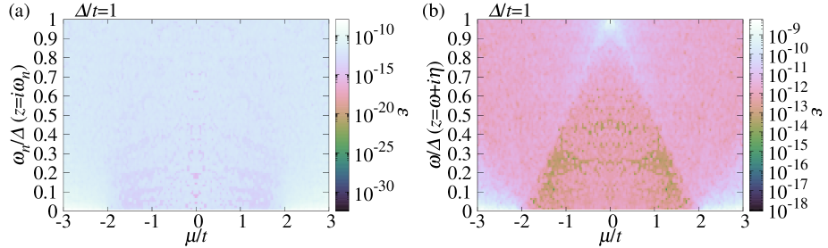
Figure S1: $\varepsilon$ for the Kitaev chain with $\Delta/t=1$ is plotted as functions of (a) $\mu/t$ and $\omega_{n}/\Delta$ ($z=\mathrm{i}\omega_{n}$) and (b) $\mu/t$ and $\omega/\Delta$ ($z=\omega+\mathrm{i}\eta$ with $\eta=10^{-2}$).

We numerically calculate $F_{\mathrm{edge}}^{\mathrm{odd}}(z)$ by using Eq. (S41) and compare it with $w_{\mathrm{bulk}}(z)/z$ [Eq. (S14)] for $t=\Delta$ and $\mu\neq 0$. When we calculate $\mathrm{Tr}_{j}$ in $F_{\mathrm{edge}}^{\mathrm{odd}}(z)$, we take $10^{4}$ sites from the surface. In Fig. S1, we show

$$\varepsilon= \frac{|F_{\mathrm{edge}}^{\mathrm{odd}}(z)-w_{\mathrm{bulk}}(z)/z|}{|w_{\mathrm{bulk}}(z)/z|}$$ (S80)

as functions of $\mu/t$ and $z/\Delta$ for $\Delta/t=1$. In Fig. S1(a), we set $z=i\omega_{n}$ and in (b), we set $z=\omega+i\eta$ ($\eta/t=10^{-2}$). The order of $\varepsilon$ is less than $10^{-8}$ for the both cases.

I.7.2 $\Delta/t=0.05$

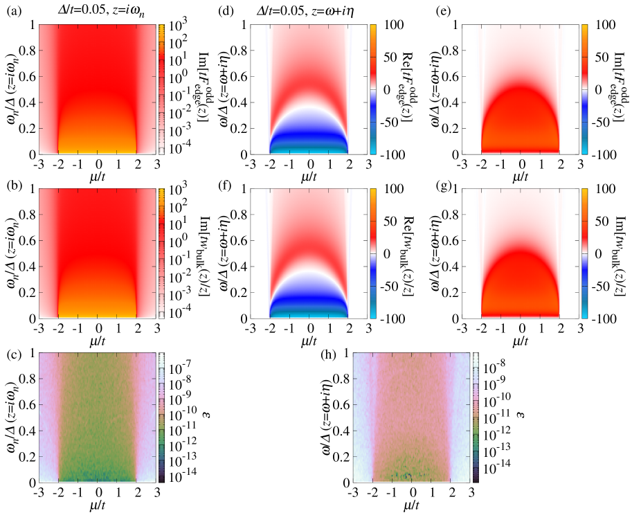
Figure S2: (a) Im$[F_{\mathrm{edge}}^{\mathrm{odd}}(z)]$, (b) Re$[w_{\mathrm{bulk}}(z)/z]$ and (c) $\varepsilon$ for Kitaev chain with $\Delta/t=0.05$ are plotted as functions of $\mu/t$ and $\omega_{n}/\Delta$ ($z=\mathrm{i}\omega_{n}$). (d) Re$[F_{\mathrm{edge}}^{\mathrm{odd}}(z)]$, (e) Im$[F_{\mathrm{edge}}^{\mathrm{odd}}(z)]$, (f) Re$[w_{\mathrm{bulk}}(z)/z]$, (g) Im$[w_{\mathrm{bulk}}(z)/z]$ and (h) $\varepsilon$ for Kitaev chain with $\Delta/t=0.1$ are plotted as functions of $\mu/t$ and $\omega/\Delta$ ($z=\omega+\mathrm{i}\eta$ with $\eta=10^{-2}$).

We numerically calculate $F_{\mathrm{edge}}^{\mathrm{odd}}(z)$ by using the recursive Green’s function method Umerski (1997) and $w_{\mathrm{bulk}}(z)/z$ by using Eq. (S11) with $\Delta/t=0.05$. When we calculate $\mathrm{Tr}_{j}$ in $F_{\mathrm{edge}}^{\mathrm{odd}}(z)$, we take $10^{5}$ sites from the surface and when we calculate integral in $w_{\mathrm{bulk}}(z)$, we also take $10^{5}$ wave numbers. In Fig. S2, we show (a) $F_{\mathrm{edge}}^{\mathrm{odd}}(z)$, (b) $w_{\mathrm{bulk}}(z)/z$ and (c) $\varepsilon$ as functions of $\mu/t$ and $\omega_{n}/\Delta$ ($z=i\omega_{n}$) for $\Delta/t=0.05$. We also show (d) Re$[F_{\mathrm{edge}}^{\mathrm{odd}}(z)]$, (e) Im$[F_{\mathrm{edge}}^{\mathrm{odd}}(z)]$, (f) Re$[w_{\mathrm{bulk}}(z)/z]$, (g) Im$[w_{\mathrm{bulk}}(z)/z]$ and (h) $\varepsilon$ as functions of $\mu/t$ and $\omega/\Delta$ ($z=\omega+i\eta$) for $\Delta/t=0.05$. The order of $\varepsilon$ is less than $10^{-6}$ for $z=i\omega_{n}$ and $10^{-7}$ for $z=\omega+i\eta$. As can be seen in Fig. S2, $\varepsilon$ becomes large where $F_{\mathrm{edge}}^{\mathrm{odd}}(z)$ and $w_{\mathrm{bulk}}(z)/z$ are small.

I.8 Spatial modulation of gap function and chemical potential

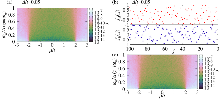
Figure S3: (a) $\varepsilon$ with surface modulation of the gap function [$\tanh(j\Delta/t)$] is plotted as functions of $\mu/t$ and $\omega_{n}/\Delta$ for $\Delta/t=0.05$. (b) randomly chosen $f_{\Delta}(j)$ and $f_{\mu}(j)$ are plotted as a function of $j$. (c) $\varepsilon$ with surface modulation shown in (b) is plotted as functions of $\mu/t$ and $\omega_{n}/\Delta$ for $\Delta/t=0.05$.

In this subsection we show that the SBBC holds even if we introduce spatial modulation of the gap function and the chemical potential near the surface. In Fig. S3(a), we show $\varepsilon$ where gap function is the form $\tanh(j\Delta/t)$. In Fig. S3(c), we show $\varepsilon$ where gap function and chemical potential are randomly chosen. In these cases the Hamiltonian with semi-infinite system is

$${\cal H}= -t\sum_{j}\left(c_{j}^{\dagger}c_{j+1}+\mathrm{H.c.}\right)+\Delta\sum_{j}f_{\Delta}(j)\left(c_{j+1}^{\dagger}c_{j}^{\dagger}+\mathrm{H.c.}\right)$$

$$-\sum_{j}\left[\mu+tf_{\mu}(j)\right]n_{j}.$$ (S81)

Note that this Hamiltonian has chiral symmetry. In Fig. S3(a), we set $f_{\Delta}(j)=\tanh(j\Delta/t)$ and $f_{\mu}(j)=1$ and in Fig. S3(c), $|f_{\Delta}(j)|<1$ and $|f_{\mu}(j)|<1$ are random values [These values are shown in Fig. S3(b)] for $j\leq 100$ and $f_{\Delta}(j)=1$ and $f_{\mu}(j)=0$ for $j>100$.

We can conclude from the numerical results in figures that the SBBC holds even when the spatial modulation near the surface is taken into account.

I.9 Exact formula of $\chi$ for Kitaev chain with any $\Delta/t>0$

To obtain $\chi$ away from the transition point, we analytically calculate $\chi$ for $\mu>0$. $\chi$ for $\mu<0$ can be obtained in a similar manner. $w_{\mathrm{bulk}}(z)$ for arbitrary $\Delta/t$ ($\Delta/t>0$) is given by Eq. (S11). Let $x=e^{\mathrm{i}k}$ be a complex number then $w_{\mathrm{bulk}}(z)$ can be written as

$$w_{\mathrm{bulk}}(z)= \frac{1}{2\pi}\int_{C}\frac{\mathrm{d}x}{\mathrm{i}x}\frac{-t\Delta-\frac{\mu\Delta}{2}(x+x^{-1})/2}{z^{2}+\Delta^{2}(x-x^{-1})^{2}/4-[-t(x+x^{-1})/2-\mu/2]^{2}},$$ (S82)

where the integral path $C$ is a unit circle in the complex plane. Then $\chi$ is obtained by the second derivative of $w_{\mathrm{bulk}}(z)$ as

$$\chi= -\frac{1}{2\pi\mathrm{i}}\int_{C}\mathrm{d}x\frac{\left[-t\Delta x-\frac{\mu\Delta}{2}(x^{2}+1)/2\right]x^{2}}{\left\{\frac{\Delta^{2}(x^{2}-1)^{2}}{4}-\left[-t(x^{2}+1)/2-\mu x/2\right]^{2}\right\}^{2}}.$$ (S83)

There are three cases.
i) $\mu=0$ and $\Delta/t=1$

There is a pole at $x=0$ and $\chi=1$ (See Eq. S15).
ii) $\mu\neq 0$ and $\Delta/t=1$

There are two poles $x=-2t/\mu$, $-\mu/2t$ and $\chi$ is given by Eq. (S15).
iii) In other cases ($\mu\neq 0$ and $\Delta/t\neq 1$)

There are four poles.

$$x= \frac{-\mu/2\pm\sqrt{\mu^{2}/4-t^{2}+\Delta^{2}}}{t\pm\Delta}.$$ (S84)

Note that poles

$$x_{++}= \frac{-\mu/2+\sqrt{\mu^{2}/4-t^{2}+\Delta^{2}}}{t+\Delta},$$ (S85)

$$x_{--}= \frac{-\mu/2-\sqrt{\mu^{2}/4-t^{2}+\Delta^{2}}}{t-\Delta},$$ (S86)

$$x_{+-}= \frac{-\mu/2+\sqrt{\mu^{2}/4-t^{2}+\Delta^{2}}}{t-\Delta},$$ (S87)

$$x_{-+}= \frac{-\mu/2-\sqrt{\mu^{2}/4-t^{2}+\Delta^{2}}}{t+\Delta},$$ (S88)

satisfy

$$x_{++}x_{--}=x_{+-}x_{-+}=1.$$ (S89)

Then there are two poles in the unit circle and we have to check which are located in the circle.

Note that $|x_{++}|<|x_{--}|$ is satisfied for all parameter range.

I.9.1 $\mu^{2}/4-t^{2}+\Delta^{2}<0$

In this case $|x_{+-}|>|x_{-+}|$ and $\mu<2t$ (QCR1 or QCR2) are satisfied and $\chi$ is

$$\chi= \chi_{1}=\frac{2t^{2}}{(\mu^{2}-4t^{2})\Delta^{2}}-2\frac{\mu^{2}+4t^{2}}{(\mu^{2}-4t^{2})^{2}}.$$ (S90)

For QCR1 ($|\Delta/(t-\mu/2)|\gg 1$), $\chi$ is given by

$$\chi\sim-2(\mu^{2}+4t^{2})\frac{1}{(\mu+2t)^{2}}\frac{1}{(\mu-2t)^{2}},$$ (S91)

and for QCR2 ($\Delta^{2}/(t^{2}-\mu^{2}/4)\ll 1$), $\chi$ is given by

$$\chi\sim\frac{2t^{2}}{\Delta^{2}}\frac{1}{\mu+2t}\frac{1}{\mu-2t}.$$ (S92)

I.9.2 $\mu^{2}/4-t^{2}+\Delta^{2}>0$

There are two cases.
1)$\mu<2t$ (QCR1 or QCR2)
QCR1 ($\Delta^{2}/(4t^{2}-\mu^{2})\gg 1$) is included in this case.

In this case, the relation $|x_{+-}|>|x_{-+}|$ holds and $\chi$ is

$$\chi= \chi_{1}\sim-2(\mu^{2}+4t^{2})\frac{1}{(\mu+2t)^{2}}\frac{1}{(\mu-2t)^{2}},$$ (S93)

2)$\mu>2t$ (QCR1 or QCR3)

In this case, the relation $|x_{+-}|<|x_{-+}|$ holds and $\chi$ is

$$\chi= \chi_{2}=\frac{\Delta\mu t/2}{(\mu^{2}/4-t^{2})^{2}\sqrt{\Delta^{2}+\mu^{2}/4-t^{2}}}.$$ (S94)

In the case $\Delta^{2}/(t^{2}-\mu^{2}/4)\gg 1$ (QCR1), $\chi_{2}$ can be expanded as

$$\chi_{2}\sim-\frac{1}{(\mu-2t)^{2}}+\mathcal{O}((\mu-2t)^{-1}).$$ (S95)

In the case $|\Delta/(t-\mu/2)|\ll 1$ (QCR3), $\chi_{2}$ can be expanded as

$$\chi_{2}\sim\frac{16\mu t\Delta}{(\mu^{2}-4t^{2})^{5/2}}-\frac{32\mu t\Delta^{3}}{(\mu^{2}-4t^{2})^{7/2}}+\mathcal{O}(\Delta^{5}).$$ (S96)

I.10 Critical exponent of $\chi$ for Kitaev chain

The low energy action for the Kitaev chain is given by

$$S=\frac{1}{2}\int\mathrm{d}\tau\mathrm{d}x\Psi^{\dagger}\left[\partial_{\tau}\tau_{0}+v\partial_{x}\tau_{2}+\left(m-\Lambda\partial_{x}^{2}\right)\tau_{3}\right]\Psi,$$ (S97)

with $\Psi=(\psi,\psi^{\dagger})^{\mathrm{T}}$. For the Kitaev chain, $v$, $m$ and $\Lambda$ are given by $v=\Delta$, $m=\delta\mu=\mu-\mu_{\mathrm{c}}$ and $\Lambda=t$, respectively, and this action describes the low-energy excitations that appear around wavevector $\pi$.

Let us consider the following scaling transformation:

$$x^{\prime}= xe^{-l},$$ (S98)

$$\tau^{\prime}= \tau e^{\dim[\tau]l},$$ (S99)

$$\psi^{\prime}= \psi e^{\dim[\psi]l},$$ (S100)

$$v^{\prime}= ve^{\dim[v]l},$$ (S101)

$$m^{\prime}= me^{\dim[m]l},$$ (S102)

The conditions for a scale-invariant action are $\dim\tau=-2$, $\dim\psi=1/2$, $\dim v=1$, and $\dim m=2$. Since $w_{\mathrm{bulk}}(z)$ is an even function of $z$, we can expand it as

$$w_{\mathrm{bulk}}(z)= \sum_{n=0}^{\infty}a_{2n}z^{2n},$$ (S103)

where $W=a_{0}$ and $\chi=a_{2}$. $w_{\mathrm{bulk}}(z)$ is dimensionless and therefore its scaling dimension is zero. As explained in the main text, $a_{2n}$ is expressed near the critical points as

$$a_{2n}\sim v^{\alpha_{n}}m^{\beta_{n}}.$$ (S104)

By applying scale transformation in Eqs. (S99), (S101) and (S102), we get

$$\alpha_{n}\dim[v]+\beta_{n}\dim[m]+2n\dim[z]=0.$$ (S105)

Here we have used the relation $\dim z=-\dim\tau$. In the general action in Eq.(S97), the relation between $\alpha_{n}$ and $\beta_{n}$ is determined by Eq. (S105), but we need more information to determine the concrete value of exponents.

To specify the functional form in more details, we consider the three quantum critical regions (QCR): $|\Delta|\gg|\delta\mu|$ (QCR1), $|\Delta|\ll|\delta\mu|$, $\delta\mu<0$ (QCR2) and $|\Delta|\ll|\delta\mu|$, $\delta\mu>0$ (QCR3). See also Fig. 4 in the main text. For QCR1, the criticality is determined by the Ising universality class, and the $\partial_{x}^{2}$ term in Eq. (S97) can be neglected in the low-energy region. In this case, the effective action is

$$\tilde{S}=\frac{1}{2}\int d^{2}\tilde{\tau}d^{2}\tilde{x}\tilde{\Psi}^{\dagger}\left[\partial_{\tilde{\tau}}\tau_{0}+\tilde{v}\tau_{2}+\tilde{m}\tau_{3}\right]\tilde{\Psi}$$ (S106)

where $\tilde{v}=v$ and $\tilde{m}=m$. The action is invariant if $\dim[\tilde{\tau}]=-1$, $\dim[\tilde{v}]=0$ and $\dim[\tilde{m}]=1$. In this regime, we can write the coefficient as $a_{2n}\sim\tilde{m}^{\beta^{\prime}_{n}}$. Then we can get $\beta^{\prime}_{n}=-2n$ from the scaling invariance of $w_{\rm bulk}$. Correspondingly, we get $\beta_{n}=-2n$, and from Eq.(S105) we get $\alpha_{n}=0$. We find the odd-frequency pair amplitude with the form

$$F_{\mathrm{edge}}^{\mathrm{odd}}(z)=z^{-1}\mathcal{W}_{1}\left(\frac{z^{2}}{\delta\mu^{2}}\right),$$ (S107)

indicating

$$\chi\sim\delta\mu^{-2}.$$ (S108)

For QCR2, we focus on the criticality that appears when $\Delta\to 0$, and then we get the behavior with respect to $\delta\mu$ by utilizing Eq. (S105). The position of low-energy excitation shifts from $k=0$ to $k=2\sqrt{|m|/\Lambda}$. The corresponding low-energy action is given by Eq. (S106) with the velocity $\tilde{v}\sim\sqrt{\Lambda m}$ and mass $\tilde{m}\sim v\sqrt{m/\Lambda}$. The scaling invariance requires $\dim[\tilde{\tau}]=-1$, $\dim[\tilde{v}]=0$ and $\dim[\tilde{m}]=1$. In this regime, we can write the coefficient as $a_{2n}\sim\tilde{m}^{\beta^{\prime\prime}_{n}}$. Then we can get $\beta^{\prime\prime}_{n}=-2n$ from the scaling invariance of $w_{\rm bulk}$, and we then get $\beta_{n}=-n$. From Eq. (S105) we also get $\alpha_{n}=-2n$. We find the odd-frequency pair amplitude with the form

$$F_{\mathrm{edge}}^{\mathrm{odd}}(z)=z^{-1}\mathcal{W}_{2}\left(\frac{tz^{2}}{\delta\mu\Delta^{2}}\right),$$ (S109)

and

$$\chi\sim\Delta^{-2}\delta\mu^{-1}.$$ (S110)

Finally we consider QCR3. In this case, we cannot construct another effective action like Eq. (S106). The simplest way to determine the critical behavior of $F_{\mathrm{edge}}^{\mathrm{odd}}(z)$ is to consider the power-counting of $\Delta$ in the concrete expression of $w_{\mathrm{bulk}}(z)$ in Eq. (S11). Taking $\Delta\to 0$, one can easily see $w_{\mathrm{bulk}}(z)\sim\Delta$, meaning $\alpha_{n}=1$ and then $\beta_{n}=-\tfrac{1}{2}-2n$. We get

$$F_{\mathrm{edge}}^{\mathrm{odd}}(z)=z^{-1}\Delta(t\delta\mu)^{-1/2}\mathcal{W}_{3}\left(\frac{z^{2}}{\delta\mu^{2}}\right),$$ (S111)

and

$$\chi\sim\Delta\delta\mu^{-5/2}.$$ (S112)

Thus the numerical results are completely interpreted in terms of the generalized scaling theory.

II Nanowire with Rashba spin-orbit interaction and Zeeman field

II.1 SBBC of nanowire

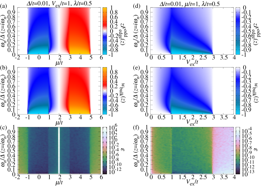
Figure S4: (a) The real part of $zF_{\mathrm{edge}}^{\mathrm{odd}}(z)$, (b) the real part of $w_{\mathrm{bulk}}(z)$, and (c) $\varepsilon$ are plotted as functions of $\mu/t$ and $\omega/\Delta$ for $\Delta/t=0.01$, $V_{\mathrm{ex}}/t=1$, and $\lambda/t=0.5$. (d) The real part of $zF_{\mathrm{edge}}^{\mathrm{odd}}(z)$, (e) the real part of $w_{\mathrm{bulk}}(z)$, and (f) $\varepsilon$ are plotted as functions of $V_{\mathrm{ex}}/t$ and $\omega/\Delta$ for $\Delta/t=0.01$, $\mu/t=1$ and, $\lambda/t=0.5$. Note that $zF_{\mathrm{edge}}^{\mathrm{odd}}(z)$ and $w_{\mathrm{bulk}}(z)$ are real valued function for purely imaginary $z$.

In this section, we numerically calculate $F_{\mathrm{edge}}^{\mathrm{odd}}(z)$ and $w_{\mathrm{bulk}}(z)/z$ for the system which is the one-dimensional $s$-wave superconductor with Rashba spin-orbit coupling and Zeeman field. The Kitaev chain does not have a spin degree of freedom but this model has it and is more complicated system. At first, we show $zF_{\mathrm{edge}}^{\mathrm{odd}}(z)$, $w_{\mathrm{bulk}}(z)$ and $\varepsilon$ for the nanowire in Fig. S4. When we calculate $\mathrm{Tr}_{j}$ in $F_{\mathrm{edge}}^{\mathrm{odd}}(z)$, we take $10^{5}$ sites from the surface and when we calculate integral in $w_{\mathrm{bulk}}(z)$, we also take $10^{5}$ wave numbers. In Figs. S4(c) and (f), $\varepsilon$ becomes large where the value of $F_{\mathrm{edge}}^{\mathrm{odd}}(z)$ and $w_{\mathrm{odd}}(z)$ are approximately zero [see Figs. S4(a), (b), (d) and (e)]. In Figs. S4(c), at $\mu/t=2$, $\varepsilon$ is very large because the order of $zF_{\mathrm{edge}}^{\mathrm{odd}}(z)$ is $10^{-11}$ and that of $w_{\mathrm{bulk}}(z)$ is $10^{-15}$ and they are almost zero.

II.2 Criticality of nanowire

The low energy effective action is given by Eq. (S97). Let $\delta\mu_{1,3}$ and $\delta V_{1,2}$ be

$$\delta\mu_{1}= \mu-\mu_{\mathrm{c}1},$$ (S113)

$$\delta\mu_{3}= \mu-\mu_{\mathrm{c}3},$$ (S114)

$$\delta V_{1}= V_{\mathrm{ex}}-V_{\mathrm{c}1},$$ (S115)

$$\delta V_{2}= V_{\mathrm{ex}}-V_{\mathrm{c}2},$$ (S116)

with $\mu_{\mathrm{c}1}=-\sqrt{V_{\mathrm{ex}}^{2}-\Delta^{2}}$, $\mu_{\mathrm{c}3}=4t-\sqrt{V_{\mathrm{ex}}^{2}-\Delta^{2}}$, $V_{\mathrm{c}1}=\sqrt{\mu^{2}+\Delta^{2}}$, and $V_{\mathrm{c}2}=\sqrt{(4t-\mu)^{2}+\Delta^{2}}$.

We only show the results near the topological quantum transition points at $\mu=\mu_{\mathrm{c}1}$, $\mu_{\mathrm{c}3}$. The critical behavior near $\mu_{\mathrm{c}2}=\sqrt{V_{\mathrm{ex}}^{2}-\Delta^{2}}$ and $\mu_{\mathrm{c}4}=4t+\sqrt{V_{\mathrm{ex}}^{2}-\Delta^{2}}$ are the same as that near $\mu_{\mathrm{c}1}$ and $\mu_{\mathrm{c}3}$, respectively. We suppose $|\Delta|\ll t$ in the following discussion.

II.2.1 Near the transition point $V_{\mathrm{ex}}=V_{\mathrm{c}1}$

(i) $|\delta\mu_{1}|\ll t$.

The constants $v$, $m$ and $\Lambda$ in Eq. (S97) are given by

$$v\sim \frac{\lambda\Delta}{V_{\mathrm{ex}}},$$ (S117)

$$m\sim \delta\mu_{1},$$ (S118)

$$\Lambda\sim \frac{\lambda^{2}}{2|\mathrm{V_{\mathrm{ex}}}|}+t.$$ (S119)

(ii) $|\delta V_{1}|\ll t$.

$v$, $m$ and $\Lambda$ in Eq. (S97) are given by

$$v\sim \frac{\lambda\Delta}{\mu},$$ (S120)

$$m\sim \delta V_{1},$$ (S121)

$$\Lambda\sim \frac{\lambda^{2}+2t\mu}{2|\mu|}.$$ (S122)

Note that the roles of the $V_{\mathrm{ex}}$ and $\mu$ in the cases (i) and (ii) are exchanged. With these coefficients, the critical behaviors can be explained based on the scaling theory described in the previous section.

II.2.2 Near the transition point $V_{\mathrm{ex}}=V_{\mathrm{c}2}$

(i) $|\delta\mu_{3}|\ll t$.

$v$, $m$ and $\Lambda$ in Eq. (S97) are given by

$$v\sim \frac{\lambda\Delta}{V_{\mathrm{ex}}},$$ (S123)

$$m\sim \delta\mu_{3},$$ (S124)

$$\Lambda\sim \frac{\lambda^{2}}{2|V_{\mathrm{ex}}|}+t.$$ (S125)

(ii) $|\delta V_{2}|\ll t$.

$v$, $m$ and $\Lambda$ in Eq. (S97) are given by

$$v\sim \frac{\lambda\Delta}{\mu-4t},$$ (S126)

$$m\sim \delta V_{2},$$ (S127)

$$\Lambda\sim \frac{\lambda^{2}-2t(\mu-4t)}{2|\mu-4t|}.$$ (S128)

II.2.3 Numerical results

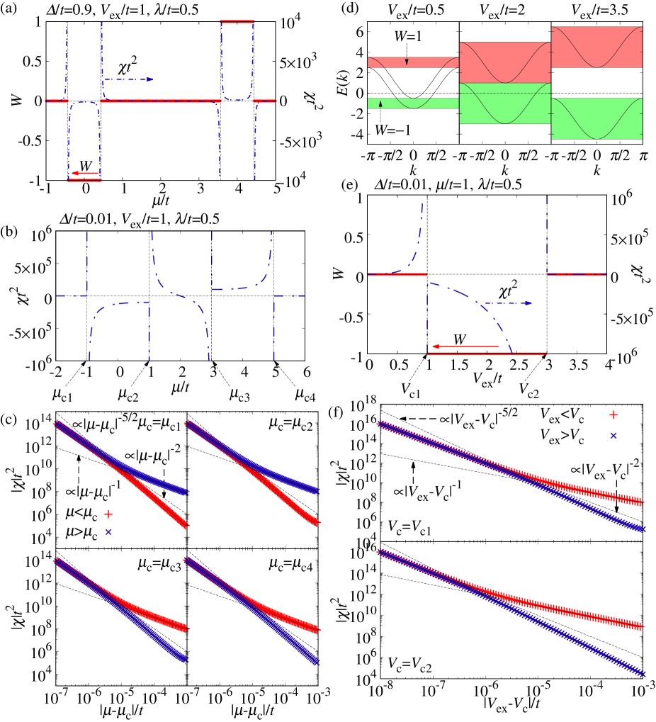
Figure S5: (a) $W$ (left vertical axis) and $\chi t^{2}$ (right vertical axis) are plotted as a function of $\mu/t$ for $\Delta/t=0.9$, $V_{\mathrm{ex}}/t=1$ and $\lambda/t=0.5$. (b) $\chi t^{2}$ is plotted as a function of $\mu/t$ for $\Delta/t=0.01$, $V_{\mathrm{ex}}/t=1$ and $\lambda/t=0.5$ with $\mu_{\mathrm{c}1}=-\sqrt{V_{\mathrm{ex}}^{2}-\Delta^{2}}$, $\mu_{\mathrm{c}2}=\sqrt{V_{\mathrm{ex}}^{2}-\Delta^{2}}$, $\mu_{\mathrm{c}3}=4t-\sqrt{V_{\mathrm{ex}}^{2}-\Delta^{2}}$, and $\mu_{\mathrm{c}4}=4t+\sqrt{V_{\mathrm{ex}}^{2}-\Delta^{2}}$. (c) $|\chi|t^{2}$ is plotted as a function of $|\mu-\mu_{\mathrm{c}}|/t$ close to $\mu=\mu_{\mathrm{c}1}$, $\mu=\mu_{\mathrm{c}2}$, $\mu=\mu_{\mathrm{c}3}$, and $\mu=\mu_{\mathrm{c}4}$. (d) Energy dispersion is plotted as a function of $k$ with $V_{\mathrm{ex}}=0.5$, $V_{\mathrm{ex}}=2$ and $V_{\mathrm{ex}}=3.5$ for $\Delta/t=0.01$, $\mu/t=1$ and $\lambda/t=0.5$. Green shaded area and red shaded one is a topological regime with $W=-1$ for green and $W=1$ for red, respectively. (e) $W$ (left vertical axis) and $\chi t^{2}$ (right vertical axis) are plotted as a function of $V_{\mathrm{ex}}/t$ for $\Delta/t=0.01$, $\mu/t=1$ and $\lambda/t=0.5$ with $V_{\mathrm{c}1}=\sqrt{\mu^{2}-\Delta^{2}}$, $V_{\mathrm{c}2}=\sqrt{{(4t-\mu)}^{2}-\Delta^{2}}$. $W$ and $\chi$ are even function of $V_{\mathrm{ex}}$. (f) $|\chi|t^{2}$ is plotted as a function of $|V_{\mathrm{ex}}-V_{\mathrm{c}}|/t$ close to $V_{\mathrm{ex}}=V_{\mathrm{c}1}$ and $V_{\mathrm{ex}}=V_{\mathrm{c}2}$.

Then we discuss about $\chi$. In Fig. S5(a), $W$ and $\chi$ are plotted as a function of $\mu/t$ for $\Delta/t=0.9$, $V_{\mathrm{ex}}/t=1$ and $\lambda/t=0.5$. As mentioned in the main text, $\chi$ diverges slower than the case with $\Delta/t=0.01$. In Fig. S5(b), $\chi/t$ is plotted as a function of $\mu/t$ and there are four topological transition points $\mu_{\mathrm{c}1}$ to $\mu_{\mathrm{c}4}$. We show $|\chi|$ near topological transition points in Fig. S5(c). The power of divergence is $|\mu-\mu_{\mathrm{c}}|^{-2}$ very close to the transition point for all topological transition points. As explained in the main text, the divergence far from transition points are $\delta\mu^{-1}$ or $\delta\mu^{-5/2}$ with $\delta\mu=\mu-\mu_{\mathrm{c}}$.

Next, we discuss about $V_{\mathrm{ex}}$ dependence of $\chi$. In Fig. S5(d) energy dispersion is plotted for $V_{\mathrm{ex}}/t=0.5$ (non-topological), $V_{\mathrm{ex}}/t=2$ (topological) and $V_{\mathrm{ex}}/t=3.5$ (non-topological) with $\Delta/t=0.01$, $\mu/t=1$ and $\lambda/t=0.5$. $W$ and $\chi$ are plotted as a function of $V_{\mathrm{ex}}$ in Fig. S5(e). There are two topological transition points $V_{\mathrm{c}1}$ and $V_{\mathrm{c}2}$. $|\chi|$ is plotted near the transition points shown in Fig. S5(f). The power of divergence is also $|V_{\mathrm{ex}}-V_{\mathrm{c}}|^{-2}$ very close to the transition point for both transition points. The divergence behavior changes if we look at far from transition point. The power of divergence is $\delta V^{-1}$ or $\delta V^{-5/2}$ with $\delta V=V-V_{\mathrm{c}}$.

III $d_{x^{2}-y^{2}}$-wave SC on square lattice

III.1 SBBC of $d_{x^{2}-y^{2}}$-wave SC

In this section we calculate $F_{\mathrm{edge}}^{\mathrm{odd}}(z)$ and $w_{\mathrm{bulk}}(z)/z$ for $d_{x^{2}-y^{2}}$-wave superconductor on a square lattice with the (11) surface.

The Hamiltonian with the periodic boundary condition is

$${\cal H}= \sum_{\mathbf{k}}C_{\mathbf{k}}^{\dagger}H(\mathbf{k})C_{\mathbf{k}},$$ (S129)

$$H(\mathbf{k})= \left[-\mu\eta_{0}+\varepsilon_{1}(\mathbf{k})\eta_{1}+\varepsilon_{2}(\mathbf{k})\eta_{2}\right]\sigma_{0}\tau_{3}$$

$$+\left[\Delta_{1}\left(\mathbf{k}\right)\eta_{1}+\Delta_{2}\left(\mathbf{k}\right)\eta_{2}\right]i\sigma_{2}i\tau_{2},$$ (S130)

with

$$\varepsilon_{1}(\mathbf{k})= -t\left[1+\cos k_{x}+\cos k_{y}+\cos(k_{x}-k_{y})\right],$$ (S131)

$$\varepsilon_{2}(\mathbf{k})= t\left[\sin k_{x}+\sin k_{y}+\sin(k_{x}-k_{y})\right],$$ (S132)

$$\Delta_{1}(\mathbf{k})= -\Delta\left[1-\cos k_{x}-\cos k_{y}+\cos(k_{x}-k_{y})\right],$$ (S133)

$$\Delta_{2}(\mathbf{k})= \Delta\left[\sin k_{x}+\sin k_{y}-\sin(k_{x}-k_{y})\right],$$ (S134)

$$C_{\mathbf{k}}= \left(c_{A,\mathbf{k},\uparrow}\>c_{B,\mathbf{k},\uparrow}\>c_{A,\mathbf{k},\downarrow}\>c_{B,\mathbf{k},\downarrow}\>\right.$$

$$\left.\hskip 14.22636ptc_{A,-\mathbf{k},\uparrow}^{\dagger}\>c_{B,-\mathbf{k},\uparrow}^{\dagger}\>c_{A,-\mathbf{k},\downarrow}^{\dagger}\>c_{B,-\mathbf{k},\downarrow}^{\dagger}\right)^{\mathrm{T}},$$ (S135)

where $\eta_{0}$ and $\sigma_{0}$ are identity matrices in sublattice space, and spin space, respectively. $\eta_{\mu}$, $\sigma_{\mu}$ and $\tau_{\mu}$ ($\mu=1,2,3$) are Pauli matrices in sublattice, spin, and particle-hole space, respectively. The unit cell used in this Hamiltonian is shown in Fig. S6 (a) The chiral operator for the bulk (periodic) system is

$$\Gamma= \eta_{0}\sigma_{2}\tau_{1}.$$ (S136)

The Hamiltonian with the (11) surface for the semi-infinite system is

$${\cal H}= C^{\dagger}\begin{pmatrix}\ddots&\ddots\\ \ddots&\hat{u}&\hat{t}\\ &\hat{t}^{\dagger}&\hat{u}&\hat{t}\\ &&\hat{t}^{\dagger}&\hat{u}\end{pmatrix}C,$$ (S137)

$$\hat{u}= \begin{pmatrix}-\mu/2&0&0&0\\ 0&-\mu/2&0&0\\ 0&0&\mu/2&0\\ 0&0&0&\mu/2\end{pmatrix},$$ (S138)

$$\hat{t}= \begin{pmatrix}-t\cos\frac{k_{y}}{2}&0&0&i\Delta\sin\frac{k_{y}}{2}\\ 0&-t\cos\frac{k_{y}}{2}&-i\Delta\sin\frac{k_{y}}{2}&0\\ 0&-i\Delta\sin\frac{k_{y}}{2}&t\cos\frac{k_{y}}{2}&0\\ i\Delta\sin\frac{k_{y}}{2}&0&0&t\cos\frac{k_{y}}{2}\end{pmatrix},$$ (S139)

with

$$C= \left(\ldots,c_{1,k_{y},\uparrow},c_{1,k_{y},\downarrow},c_{1,-k_{y},\uparrow}^{\dagger},c_{1,-k_{y},\downarrow}^{\dagger}\right)^{\mathrm{T}}.$$ (S140)

The chiral operator for the semi-infinite system is

$$\Gamma= \mathrm{diag}(\ldots,\sigma_{2}\tau_{1},\sigma_{2}\tau_{1}).$$ (S141)

In Fig. S6(b), we show $F_{\mathrm{edge}}^{\mathrm{odd}}(z)$ for $\Delta/t=0.1$ and $\mu/t=-1$ and it is odd function of $k_{y}$. When we calculate $\mathrm{Tr}_{j}$ in $F_{\mathrm{edge}}^{\mathrm{odd}}(z)$, we take $10^{4}$ sites from the surface and when we calculate integral in $w_{\mathrm{bulk}}(z)$, we also take $10^{4}$ wave numbers. $\varepsilon$ is plotted as functions of $k_{y}$ and $\omega_{n}/\Delta$ in Fig. S6(c) and is less than $10^{-7}$. At $k_{y}=0$, there is no value because $F_{\mathrm{edge}}^{\mathrm{odd}}(z)$ and $w_{\mathrm{bulk}}(z)$ are exactly zero. In Fig. S6(d), we show $W$ and $\chi$ as a function of $k_{y}$ and there are three topological transition points 0 and $\pm 2\arccos(-\mu/4t)$.

III.2 Criticality of $d_{x^{2}-y^{2}}$-wave SC

There are three topological transition points: $k_{y}=0$ and $k_{y}=\pm k_{\mathrm{c}}$ with $k_{\mathrm{c}}=2\arccos(-\mu/4t)$.

III.2.1 Criticality at $k_{y}=\pm k_{c}$

The effective low energy action near $k_{y}=\pm k_{\mathrm{c}}$ is given by Eq. (S97) with

$$v\sim \Delta\sqrt{4-\frac{\mu^{2}}{4t^{2}}},$$ (S142)

$$m\sim t^{2}\delta k\sqrt{4-\frac{\mu^{2}}{4t^{2}}},$$ (S143)

$$\Lambda\sim \frac{\mu}{8},$$ (S144)

with $\delta k=k_{x}-k_{\mathrm{c}}$. The scaling behavior can be understood based on Eq. (S97) as in the previous sections.

III.2.2 Criticality at $k_{y}=0$

The effective low energy action near $k_{y}=0$ is given by

$$S= \frac{1}{2}\int\mathrm{d}\tau\mathrm{d}x\Psi^{\dagger}\left[\partial_{\tau}\tau_{0}+\tilde{v}\partial_{x}\tau_{3}+\tilde{m}\tau_{1}\right]\Psi,$$ (S145)

with

$$\tilde{v}\sim 2t\sin\left(\frac{k_{\mathrm{c}}}{2}\right),$$ (S146)

$$\tilde{m}\sim 2k_{y}\Delta\sin\left(\frac{k_{\mathrm{c}}}{2}\right).$$ (S147)

Then by using scale transformation, we get

$$\dim[\tau]= -1,$$ (S148)

$$\dim[\psi]= 1/2,$$ (S149)

$$\dim[k_{y}]= 1/2,$$ (S150)

$$\dim[\Delta]= 1/2.$$ (S151)

Here we use the fact that $k_{y}$ and $\Delta$ are symmetric in the effective action. Then the generalized winding number can be expanded as

$$w_{\mathrm{bulk}}(z)\sim\sum_{n}\tilde{a}_{2n}{(k_{y}\Delta)}^{\gamma_{n}}z^{2n}.$$ (S152)

By using scale transformation, we obtain

$$2n\dim[z]+\gamma_{n}\left(\dim[k_{y}]+\dim[\Delta]\right)=0,$$

$$\Leftrightarrow 2n+\gamma_{n}=0.$$ (S153)

Then the generalized winding number is obtained as

$$w_{\mathrm{bulk}}(z)\sim \sum_{n}\tilde{a}_{2n}(k_{y}\Delta)^{-2n}z^{2n},$$ (S154)

and $\chi$ behaves as

$$\chi\sim (k_{y}\Delta)^{-2}.$$ (S155)

$|\chi|$ is shown in Figs. S6(e) near $k_{y}=0$ and (f) near $k_{y}=k_{\mathrm{c}}$. In both cases, close to the quantum transition point, the power of the divergence is $k_{y}^{-2}$ and $|k_{y}-k_{\mathrm{c}}|^{-2}$, respectively. Away from the transition point $k_{y}=k_{\mathrm{c}}$, the power of divergence is $(k_{y}-k_{\mathrm{c}})^{-1}$ [$(k_{y}-k_{\mathrm{c}})^{-5/2}$] for $k_{y}<k_{\mathrm{c}}$ ($k_{y}>k_{\mathrm{c}}$).

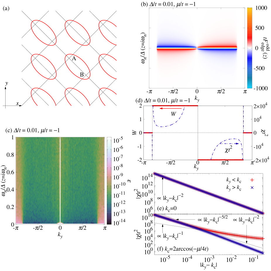
Figure S6: (a)Schematic illustration of the unit cell. A and B indicate sublattices. (b) Imaginary part of $F_{\mathrm{edge}}^{\mathrm{odd}}(z)$ is plotted as functions of $k_{y}$ and $\omega_{n}/\Delta$ with $\Delta/t=0.01$ and $\mu/t=-1$. (c) $\varepsilon$ is plotted as functions of $k_{y}$ and $\omega_{n}/\Delta$ with $\Delta/t=0.01$ and $\mu/t=-1$. At $k_{y}=0$, there is no value because $w_{\mathrm{bulk}}(z)$ and $F_{\mathrm{edge}}^{\mathrm{odd}}(z)$ are exactly zero. (d) $\chi t^{2}$ is plotted as a function of $k_{y}$. $|\chi|t^{2}$ is plotted as a function of $|k_{y}-k_{\mathrm{c}}|$ near (e) $k_{\mathrm{c}}=0$ and (f) $k_{\mathrm{c}}=2\arccos(-\mu/4t)$. Dotted lines in (b) and (c) are proportional to $|k_{y}-k_{\mathrm{c}}|^{-2}$.

References

PG (8)See for e.g., “The Quantum Hall
Effect”, edited by R.E. Prange anS.M. Girvin, (Springer-Verlag, 1987), and
references therein.
G.R.Volovik (2003)G.R.Volovik, “The Universe in a Helium Droplet,” (Oxford Science Publications, 2003).
Hasan and Kane (2010)M. Z. Hasan and C. L. Kane, Rev.
Mod. Phys. 82, 3045
(2010).
Ryu and Hatsugai (2002)S. Ryu and Y. Hatsugai, Phys. Rev. Lett. 89, 077002 (2002).
Di Bernardo et al. (2015)A. Di Bernardo, Z. Salman,
X. L. Wang, M. Amado, M. Egilmez, M. G. Flokstra, A. Suter, S. L. Lee, J. H. Zhao, T. Prokscha,
E. Morenzoni, M. G. Blamire, J. Linder, and J. W. A. Robinson, Phys. Rev. X 5, 041021 (2015).
Linder and Balatsky (2017)J. Linder and A. V. Balatsky, arXiv:1709.09386 (2017).