On Stability of a Class of Filters for Non-Linear Stochastic Systems

Abstract

This article develops a comprehensive framework for stability analysis of a broad class of commonly used continuous and discrete time-filters for stochastic dynamic systems with non-linear state dynamics and linear measurements under certain strong assumptions. The class of filters encompasses the extended and unscented Kalman filters and most other Gaussian assumed density filters and their numerical integration approximations. The stability results are in the form of time-uniform mean square bounds and exponential concentration inequalities for the filtering error. In contrast to existing results, it is not always necessary for the model to be exponentially stable or fully observed. We review three classes of models that can be rigorously shown to satisfy the stringent assumptions of the stability theorems. Numerical experiments using synthetic data validate the derived error bounds.

37N35, 60G35, 60H10, 93B05, 93B07, 93D20, 93E15

1 Introduction

Non-linear Kalman filters, such as the extended Kalman filter (EKF), the derivative-free unscented Kalman filter (UKF), and other Gaussian integration filters, are fundamental tools widely used in estimating a latent time-evolving state from partial and noisy measurements in, for instance, automatic control, robotics, and signal processing [44]. These filters are local extensions to the classical linear Kalman filter for systems with non-linear state evolution or measurement equation. Stability properties of the optimal linear Kalman filter are well understood, having been extensively studied since the 1960s in continuous [12, 21, 6] and discrete time [22, 24, 1] settings. However, most systems of interest are non-linear, and non-linear extensions of the Kalman filter inherit no global optimality properties. Even though these filters tend to provide useful estimates, analyzing their stability is far from trivial.

This article analyzes stochastic stability, defined as time-uniform boundedness of the mean square filtering error, of a large class of extensions of the Kalman filter for systems with non-linear state dynamics and linear measurements. Our main stability results, Theorems 3.1 and 4.2, provide time-uniform mean square filtering error bounds and related exponential concentration inequalities for a large class of filters. The theorems significantly extend the recent results by Del Moral et al. [19] on the EKF for exponentially stable (i.e., contractive) and fully observed models. The most important extensions are of three types: (a) we formulate an apparently novel framework that allows for considering a large class of commonly used filters simultaneously, not just the EKF; (b) we do not require that the model be exponentially stable or fully observed; and (c) we also cover the discrete-time case. In practice, generalization (b) is enabled by introduction of a certain assumption on stability of the filter process. That this assumption is satisfied by some classes of models not exponentially stable nor fully observed, and thus beyond the scope of applicability of [19] even when the EKF is used, is demonstrated in Section 5. Even though the stability assumptions used in this article are extremely restrictive and essentially amount to stability of the filtering error process, we stress that they are, as far as we are aware of, the least restrictive among assumptions used in the literature that permit rigorous a priori assessment of stability. A more detailed presentation of our contributions is provided in Section 1.2.

There are two underlying objectives in this article that are not present in most previous works:

• Our stability analysis is general and unified in that the class of filters it applies to encompasses most non-linear Kalman filters commonly used in relatively low-dimensional applications, such as tracking. Ensemble Kalman filters, useful in high-dimensional applications, have been recently analyzed in [16, 18].

• We require that stability be rigorously a priori verifiable and the error bounds a priori computable. This means that it should be possible to conclude that a filter is stable and compute mean square error bounds before the filter is run. Accordingly, three classes of models for which this is possible are reviewed in Section 5. These requirements are in contrast to much of the existing literature where the results rely on opaque and difficult-to-verify assumptions [54, 33] or no example models are provided that can be rigorously shown to satisfy the assumptions [37, 38, 30].

The second objective is crucial if stability results are to be applied in practice and is in some contrast to earlier work where it is occasionally suggested that (a) having values of certain parameters, as computed when the filter is run, satisfy the bounds or conditions required for stability allows for concluding that a stochastic filter is stable (e.g., [37, p. 716] and [53, p. 244]), which is problematic if one is considering stability in mean square sense since the conditions are validated only for one particular trajectory, though more acceptable in the deterministic setting [9, p. 566], or that (b) the true state can be assumed to remain in a compact set (see [37, Theorem 4.1] and [7]). A consequence of this is that we work only with linear measurement models. However, it should be noted that, out of necessity, many models that have been previously used in demonstrating stability results have linear measurements; see for example the model examined in [37, 54].

1.1 Previous Work and Technical Aspects

A Kalman filter or its non-linear extension provides, at time $t\geq 0$, an online estimate $\widehat{X}_{t}$ constructed out of a potentially partial and noisy measurement sequence $\{Y_{s}\}_{s=0}^{t}$ of the true latent state $X_{t}$ of a dynamic system. The estimates are typically accompanied with positive-semidefinite matrices $P_{t}$, which are estimates of covariances of the estimation errors $E_{t}=X_{t}-\widehat{X}_{t}$. These matrices and the associated gain matrices $K_{t}$ are computed from a Riccati-type differential equation. Stability of extensions of the Kalman filter for non-linear systems can be analyzed either in a deterministic or stochastic setting. In the former case, the state dynamics and measurements are noiseless and the positive-semidefinite matrices $Q$ and $R$, which in the stochastic case would be covariances of Gaussian state and measurement noise terms, are tuning parameters. The goal is to prove that the estimation error converges to zero as $t\to\infty$. In the stochastic setting it cannot be expected that the error vanishes, and one instead (for example) attempts to prove time-uniform upper bounds or concentration inequalities for the mean square estimation error, $\mathbb{E}(\mathinner{\lVert E_{t}\rVert}^{2})$.

There is a large body of literature on stability properties, both in continuous and discrete time, of the EKF as a non-linear observer [39, 32, 11, 40, 41, 31, 34, 9, 4] and in the stochastic setting [37, 38, 36, 7, 30, 19] and of the UKF and related filters [54, 55, 50, 52, 53, 33, 27]. However, majority of these articles attempt to be too general, which often results in the use of assumptions that are effectively impossible to verify, especially before the filter is actually run, or in a lack of discussion on and examples of models for which the assumptions hold. There are two principal sources of difficulty in the stability analysis of non-linear filters:

Time-uniform bounds on $\boldsymbol{P_{t}}$

Analysis in most of the above articles is similar to the standard stability analysis for linear models [22, 24] in that use is made of the Lyapunov function ${V_{t}=E_{t}^{\mathsf{T}}P_{t}^{-1}E_{t}}$ or its variants. Once stability results have been obtained for $V_{t}$, time-uniform bounds on $P_{t}$ are necessary for concluding stability of the filter. While in the linear case $P_{t}$ is deterministic and bounds on this matrix follow from results on Riccati equations under certain observability and controllability conditions, in the non-linear case the local structure of most Kalman filters, arising from linearizations of some sort around the estimated trajectory, introduces a dependency of $P_{t}$ on the measurements and estimates. Consequently, the behavior of $P_{t}$ is difficult, if not impossible, to anticipate and control for most non-linear models and filters.

Model non-linearity

If the system is non-linear, stability analysis of a Kalman filter necessarily involves analyzing non-linear (stochastic) differential equations. This is obviously much more involved than analysis of linear differential equations. As such, the approach taken in many articles is to assume that the error associated to the linearization method used in a particular non-linear Kalman filter is “small”. This allows for deriving a linear differential inequality for the Lyapunov function that can be easily controlled.

When not outright assumed, boundedness of $P_{t}$ has been addressed essentially in two ways. If the system is fully observed, that is, $\operatorname{d\!}Y_{t}=X_{t}\operatorname{d\!}t+R^{1/2}\operatorname{d\!}V_{t}$, there is hope for the Riccati equation to be well behaved despite the fact it depends on $\widehat{X}_{t}$ since, essentially, the quadratic correction term in the Riccati equation prevents $\widehat{X}_{t}$ and $P_{t}$ from drifting indefinitely; see [30, Section IV] and [33, Section 4] for the discrete and [26] for the continuous-time case. Alternatively, one can consider certain difficult-to-verify non-linear extensions of the standard observability and controllability conditions [3, 37, 38, 31]. Another situation of interest is when the estimates are explicitly known to remain in a bounded region of the state space, which provides some control over the estimate-dependent terms in the Riccati equation and limits the possible values of $P_{t}$. See for example [7] where stochastic stability of the EKF in a robotics application is considered. Model non-linearity is often dealt with by enforcing Lipschitz-type bounds on the remainder related to the particular linearization method used [37, 38] or by assuming boundedness of certain residual-correcting random matrices [54, 53, 33]. However, such assumptions tend to be difficult to verify.

1.2 Contributions

This article follows the approach taken recently by Del Moral et al. [19]. They study stochastic stability of the extended Kalman–Bucy filter by directly considering the squared error $\mathinner{\lVert E_{t}\rVert}^{2}$ for which they derive stochastic differential inequalities that in turn establish time-uniform mean square error bounds and exponential concentration inequalities. However, the class of systems they consider is very restricted as they need to assume that the state is fully observed and the dynamic model, as specified by the drift function, is exponentially stable (i.e., the deterministic homogeneous differential equation $\partial_{t}x_{t}=f(x_{t})$ defined by the drift $f$ is exponentially stable). In Theorems 3.1 and 4.2 we introduce several significant generalizations and improvements to the results in [19]:

1. We consider a broad class, defined in Section 2, of generic Kalman-type filters for continuous-time non-linear systems when the measurements are linear; see (3) for the model. As demonstrated in Section 2.5, this class of filters contains many commonly used filters, including the extended Kalman–Bucy filter and the more recent Gaussian integration filters such as the unscented Kalman–Bucy filter [25, 43] and the Gauss–Hermite filter [51, 46]. This unified framework is exceedingly convenient as every filter does not have to be analyzed individually. There have been prior attempts at establishing a unified stability analysis [50, 52, 27], but the formulations are somewhat unnatural, being in terms of certain residual terms that are difficult to control.

2. Unlike in [19], the system is not explicitly required to be exponentially stable or fully observed. While still very stringent, the assumption we use is satisfied by a larger class of models (for discussion on the assumptions, see Section 3). Two model and filter classes which do not require exponential stability or full observability are reviewed in Sections 5.2 and 5.3.

3. Although our main focus is on continuous-time systems, Section 4 contains analogous results for the discrete-time case. The discrete case is instructive in demonstrating rigorously that under appropriate conditions a non-linear Kalman filter improves upon the trivial estimator $\widehat{X}_{Y,k}=Y_{k}$. This is discussed in Section 4.4.

4. Section 6 contains two numerical examples that demonstrate conservativeness of the derived mean square error bounds. Unlike in much of the literature (e.g., [37, Section V] and [38, Section 5]), we can verify beforehand that the example models satisfy the stability assumptions.

Although some elements of the proofs are similar to those in [19], inclusion of complete and self-contained proofs is necessary because our adoption of a general class of filters introduces modifications, some of the constants involved are different, and also the discrete case, for which the analysis has not been carried out before, is considered.

2 Non-Linear Systems and Filtering

This section introduces the continuous-time stochastic dynamic systems and the class of stochastic Kalman–Bucy filters the results in Section 3 apply to. A number of prominent members of this filter class are also given. Discrete-time systems and filters are discussed in Section 4.

2.1 Logarithmic Norms and Lipschitz Constants

The smallest and largest eigenvalues of a symmetric real matrix $A$ are $\lambda_{\text{min}}(A)$ and $\lambda_{\text{max}}(A)$. The logarithmic norm $\mu(A)$ of a square matrix $A\in\mathbb{R}^{d\times d}$ is ${\mu(A)=\frac{1}{2}\lambda_{\text{max}}(A+A^{\mathsf{T}})}$, coinciding with $\lambda_{\text{max}}(A)$ when $A$ is symmetric. We also define the quantity ${\nu(A)=\frac{1}{2}\lambda_{\text{min}}(A+A^{\mathsf{T}})=-\mu(-A)}$. Basic results that we repeatedly use are

$$\nu(A)\mathinner{\lVert x\rVert}^{2}\leq\langle x,Ax\rangle=x^{\mathsf{T}}Ax\leq\mu(A)\mathinner{\lVert x\rVert}^{2}$$

for any $x\in\mathbb{R}^{d}$ and the “triangle inequalities”

$$\lambda_{\text{max}}(A+B) \leq\lambda_{\text{max}}(A)+\lambda_{\text{max}}(B), \lambda_{\text{min}}(A+B) \geq\lambda_{\text{min}}(A)+\lambda_{\text{min}}(B),$$

$$\mu(A+B) \leq\mu(A)+\mu(B), \nu(A+B) \geq\nu(A)+\nu(B).$$

For a positive-semidefinite $B$, recall also the trace inequality [5, Chapter 8]

(1) $$\nu(A)\operatorname{tr}(B)\leq\operatorname{tr}(AB)\leq\mu(A)\operatorname{tr}(B)$$

for any square matrix $A$ and its special case $\lambda_{\text{min}}(A)\operatorname{tr}(B)\leq\operatorname{tr}(AB)\leq\lambda_{\text{max}}(A)\operatorname{tr}(B)$ for a symmetric $A$. See [42, 47] for detailed reviews of the logarithmic norm.

Let $g\colon\mathbb{R}^{d}\to\mathbb{R}^{d}$ be differentiable and ${[J_{g}]_{ij}=\partial g_{i}/\partial z_{j}}$ its Jacobian matrix. The Lipschitz constant of $g$ is $\mathinner{\lVert J_{g}\rVert}=\sup_{x\in\mathbb{R}^{d}}\mathinner{\lVert J_{g}(x)\rVert}$, where the matrix norm is the norm induced by the Euclidean norm (i.e., the spectral norm). This constant satisfies $\mathinner{\lVert g(x)-g(x^{\prime})\rVert}\leq\mathinner{\lVert J_{g}\rVert}\mathinner{\lVert x-x^{\prime}\rVert}$ for any $x,x^{\prime}\in\mathbb{R}^{d}$. If $\mathinner{\lVert J_{g}\rVert}<\infty$, the function $g$ is Lipschitz. The logarithmic Lipschitz constants of $g$ are

$$N(g)=\inf_{z\in\mathbb{R}^{d}}\nu[J_{g}(z)]\hskip 8.5359pt\text{and}\hskip 8.5359ptM(g)=\sup_{z\in\mathbb{R}^{d}}\mu[J_{g}(z)].$$

These constants satisfy

(2) $$N(g)\mathinner{\lVert x-x^{\prime}\rVert}^{2}\leq\big{\langle}x-x^{\prime},g(x)-g(x^{\prime})\big{\rangle}\leq M(g)\mathinner{\lVert x-x^{\prime}\rVert}^{2},$$

for any $x,x^{\prime}\in\mathbb{R}^{d}$. Note that $M(g)\leq\mathinner{\lVert J_{g}\rVert}$ [47, Proposition 3.1].

2.2 System Description

We consider systems of stochastic differential equations of the form

(3a) $$\operatorname{d\!}X_{t} =f(X_{t})\operatorname{d\!}t+Q^{1/2}\operatorname{d\!}W_{t},$$

(3b) $$\operatorname{d\!}Y_{t} =HX_{t}\operatorname{d\!}t+R^{1/2}\operatorname{d\!}V_{t},$$

where $X_{t}\in\mathbb{R}^{d_{x}}$ is the latent state evolving according to a continuously differentiable and potentially non-linear drift $f\colon\mathbb{R}^{d_{x}}\to\mathbb{R}^{d_{x}}$. We assume that the drift is Lipschitz (i.e., $\mathinner{\lVert J_{f}\rVert}<\infty$) and that its Jacobian is bounded in logarithmic norm:

(4) $$-\infty<N(f)=\inf_{x\in\mathbb{R}^{d_{x}}}\nu[J_{f}(x)]\quad\text{ and }\quad M(f)=\sup_{x\in\mathbb{R}^{d_{x}}}\mu[J_{f}(x)]<\infty.$$

These conditions ensure that the state and the filters defined later in this section remain almost surely bounded in finite time. The measurements $Y_{t}\in\mathbb{R}^{d_{y}}$ are obtained linearly through a measurement model matrix $H\in\mathbb{R}^{d_{y}\times d_{x}}$. Both the state and measurements are disturbed by independent multivariate Brownian motions $W_{t}\in\mathbb{R}^{d_{x}}$ and $V_{t}\in\mathbb{R}^{d_{y}}$ multiplied by positive-definite noise covariance matrices $Q\in\mathbb{R}^{d_{x}\times d_{x}}$ and $R\in\mathbb{R}^{d_{y}\times d_{y}}$. The state is initialized from $X_{0}\sim\mathcal{N}(\mu_{0},\Sigma_{0})$ for some mean $\mu_{0}\in\mathbb{R}^{d_{x}}$ and a positive-definite covariance $\Sigma_{0}\in\mathbb{R}^{d_{x}\times d_{x}}$.

The results of this article remain valid if the time-invariant function $f$ and matrices $H$, $Q$, and $R$ in (3) are replaced with time-varying versions that satisfy appropriate regularity and uniform boundedness conditions. For instance, with a time-varying drift $f_{t}$ the assumptions (4) become

$$-\infty<\inf_{t\geq 0}\,\inf_{x\in\mathbb{R}^{d_{x}}}\nu[J_{f_{t}}(x)]\quad\text{ and }\quad\sup_{t\geq 0}\,\sup_{x\in\mathbb{R}^{d_{x}}}\mu[J_{f_{t}}(x)]<\infty.$$

Later in Theorem 3.1 the crucial assumption (13) would be replaced with

$$\sup_{t\geq T}M(f_{t}-P_{t}S_{t})\leq-\lambda<0,$$

where $S_{t}=H_{t}R_{t}^{-1}H_{t}$ is a time-varying version of the matrix $S$ in (6), and $\operatorname{tr}(Q)$ and $\operatorname{tr}(S)$ on the right-hand side of the mean square error bound (15) would become $\sup_{t\geq T}\operatorname{tr}(Q_{t})$ and $\sup_{t\geq T}\operatorname{tr}(S_{t})$. We work in the time-invariant setting in order to keep the notation simpler.

2.3 The Extended Kalman–Bucy Filter

The extended Kalman–Bucy filter (EKF) is a classical method for computing estimates $\widehat{X}_{t}$ of the latent state $X_{t}$ of the system (3). The EKF is based on local first-order linearizations around the estimated states. It is defined by the equations

(5a) $$\operatorname{d\!}\widehat{X}_{t} =f(\widehat{X}_{t})\operatorname{d\!}t+P_{t}H^{\mathsf{T}}R^{-1}\big{(}\operatorname{d\!}Y_{t}-H\widehat{X}_{t}\operatorname{d\!}t\big{)},$$

(5b) $$\partial_{t}P_{t} =J_{f}(\widehat{X}_{t})P_{t}+P_{t}J_{f}(\widehat{X}_{t})^{\mathsf{T}}+Q_{\text{tu}}-P_{t}SP_{t},$$

where

(6) $$K_{t}=P_{t}H^{\mathsf{T}}R^{-1}\hskip 14.22636pt\text{and}\hskip 14.22636ptS=H^{\mathsf{T}}R^{-1}H,$$

the former of which are known as Kalman gain matrices. Equation (5b) governing evolution of $P_{t}$ is known as the (non-linear) Riccati equation. The matrix $Q_{\text{tu}}$ is a positive-definite matrix that does not have to be equal to $Q$, the state noise covariance, in which case we can speak of tuning this matrix [8]. The rest of this section introduces a framework for generalized Kalman-type filters similar in structure to the EKF and amenable to a unified stability analysis.

2.4 A Class of Generic Filters for Non-Linear Systems

A filter computes a quantity $\widehat{X}_{t}\in\mathbb{R}^{d_{x}}$ that is used as an estimate of the latent state $X_{t}$. We consider generic filters defined as

(7) $$\operatorname{d\!}\widehat{X}_{t}=\mathcal{L}_{\widehat{X}_{t},P_{t}}(f)\operatorname{d\!}t+P_{t}H^{\mathsf{T}}R^{-1}\big{(}\operatorname{d\!}Y_{t}-H\widehat{X}_{t}\operatorname{d\!}t\big{)},$$

where $\mathcal{L}_{x,P}$ is a parametrized linear functional, to be discussed in detail below, that maps functions $g\colon\mathbb{R}^{d_{x}}\to\mathbb{R}^{d_{x}}$ to $\mathbb{R}^{d_{x}}$ and the matrices $P_{t}\in\mathbb{R}^{d_{x}\times d_{x}}$ are user-specified, can depend on all the system parameters as well as all preceding measurements and state estimates, and are measurable with respect to the $\sigma$-algebra $\mathcal{F}_{t}=\sigma(Y_{s},s\leq t)$ generated by the measurements. An assumption that $P_{t}$ is sufficiently regular and well-behaved and Lipschitzianity in $x$ and $P$ of $\mathcal{L}_{x,P}(f)$ guarantee the existence of a unique solution to (7). Explicit examples of filters follow in Section 2.5. We initialize the filter (7) with a deterministic $\widehat{X}_{0}=\hat{x}_{0}\in\mathbb{R}^{d_{x}}$ and a positive-definite $P_{0}\in\mathbb{R}^{d_{x}\times d_{x}}$. These do not have to be equal to $\mu_{0}$ or $\Sigma_{0}$, respectively, the mean and covariance of the initial state $X_{0}$. In Section 3 we will see that, as long as they remain uniformly bounded, the construction of the matrices $P_{t}$ does not substantially affect our analysis.

The linear functional $\mathcal{L}_{x,P}$ is parametrized by $x\in\mathbb{R}^{d_{x}}$ and $P\in\mathbb{R}^{d_{x}\times d_{x}}$ and it is required that the functional

1. is Lipschitz (and hence continuous) in the parameters $x$ and $P$ in the sense that $\mathcal{L}_{x,P}(g)$ is a Lipschitz function from $\mathbb{R}^{d_{x}}\times\mathbb{R}^{d_{x}\times d_{x}}$ to $\mathbb{R}^{d_{x}}$ for any fixed Lipschitz function $g\colon\mathbb{R}^{d_{x}}\to\mathbb{R}^{d_{x}}$;

2. satisfies $\mathcal{L}_{x,P}(g)=g(x)$ for any $x$ and $P$ if $g(x)=Ax+b$ for some $A\in\mathbb{R}^{d_{x}\times d_{x}}$ and $b\in\mathbb{R}^{d_{x}}$.

Note that it is not necessary for $\mathcal{L}_{x,P}$ to depend on $P$; a prototypical example is the standard point evaluation functional $\mathcal{L}_{x,P}^{\text{\tiny{EKF}}}(g)=g(x)$ for any $P$. Another functional that is used in this article is the Gaussian integration functional

$$\begin{split}\mathcal{L}_{x,P}^{\text{\tiny{ADF}}}(g)&=\int_{\mathbb{R}^{d_{x}}}g(z)\mathcal{N}(z\mid x,P)\operatorname{d\!}z\\ &\coloneqq(2\pi)^{-d_{x}/2}\det(P)^{-1/2}\int_{\mathbb{R}^{d_{x}}}g(z)\exp\bigg{(}\!\!-\frac{1}{2}(z-x)^{\mathsf{T}}P^{-1}(z-x)\bigg{)}\operatorname{d\!}z.\end{split}$$

The above requirements on $\mathcal{L}_{x,P}$ are usually easily verifiable and non-restrictive. The following less straightforward assumption is crucial to the stability analysis in Section 3.

Assumption .

For any differentiable $g\colon\mathbb{R}^{d_{x}}\to\mathbb{R}^{d_{x}}$ with finite $N(g)$ and $M(g)$ there is a constant $C_{g}\geq 0$, which varies continuously with $M(g)$ and $N(g)$, such that

$$\big{\langle}x-\tilde{x},g(x)-\mathcal{L}_{\tilde{x},P}(g)\big{\rangle}\leq M(g)\mathinner{\lVert x-\tilde{x}\rVert}^{2}+C_{g}\operatorname{tr}(P)$$

for any $x,\tilde{x}\in\mathbb{R}^{d_{x}}$ and $P\in\mathbb{R}^{d_{x}\times d_{x}}$.

Since $\langle x-{\tilde{x}},g(x)-g({\tilde{x}})\rangle\leq M(g)\mathinner{\lVert x-{\tilde{x}}\rVert}^{2}$ by (2), what the above assumption essentially entails is that $\mathcal{L}_{\tilde{x},P}(g)$ cannot deviate too much from $g(\tilde{x})$ and that magnitude of their difference is controlled by the size of $P$.

The class of filters of the form (7) that use a linear functional satisfying Section 2.4 is very large. It encompasses, for example, the extended Kalman–Bucy filter and Gaussian assumed density filters and their most popular numerical integration approximations. Next we review a few such examples, demonstrating in the process that Section 2.4 is indeed reasonable and fairly natural.

2.5 Kalman–Bucy Filters for Continuous-Time Non-Linear Systems

A Kalman–Bucy filter for the model (3) computes approximations $\widehat{X}_{t}$ and $P_{t}$, latter of which is called error covariance in this setting, to the conditional filtering means and covariances $\mathbb{E}(X_{t}\mid\mathcal{F}_{t})$ and $\operatorname{Var}(X_{t}\mid\mathcal{F}_{t})$, respectively. It is usually difficult to derive tractable expressions for these quantities unless $f$ is affine. A generalized Kalman–Bucy filter for the model (3) is

(8a) $$\operatorname{d\!}\widehat{X}_{t} =\mathcal{L}_{\widehat{X}_{t},P_{t}}(f)\operatorname{d\!}t+P_{t}H^{\mathsf{T}}R^{-1}\big{(}\operatorname{d\!}Y_{t}-H\widehat{X}_{t}\operatorname{d\!}t\big{)},$$

(8b) $$\partial_{t}P_{t} =\mathcal{R}_{\widehat{X}_{t},P_{t}}(f)+\mathcal{R}_{\widehat{X}_{t},P_{t}}(f)^{\mathsf{T}}+Q_{\text{tu}}-P_{t}SP_{t},$$

where the linear functional $\mathcal{R}_{x,P}$ maps functions to $d_{x}\times d_{x}$ matrices. A unique solution to (8b) exists if $\mathcal{R}_{x,P}(f)$ is Lipschitz in $x$ and $P$. This holds typically when the Jacobian of $f$ satisfies $\mathinner{\lVert J_{f}(x)-J_{f}(x^{\prime})\rVert}\leq L\mathinner{\lVert x-x^{\prime}\rVert}$ for some $L<\infty$ and all $x,x^{\prime}\in\mathbb{R}^{d_{x}}$. Examples of commonly used $\mathcal{R}_{x,P}$ appear below. As in the case of the EKF, we call (8b) a Riccati equation and $Q_{\text{tu}}$ is a positive-definite tuning matrix. As we shall see, proper tuning (in practice, inflation) is often necessary to induce provable stability of a Kalman–Bucy filter. Next we provide three examples of classical Kalman–Bucy filters of the form (8) that satisfy the assumptions in Section 2.4.

2.5.1 Extended Kalman–Bucy Filter

By selecting $\mathcal{L}_{x,P}(g)=\mathcal{L}_{x,P}^{\text{\tiny{EKF}}}(g)=g(x)$ and $\mathcal{R}_{x,P}(g)=\mathcal{R}_{x,P}^{\text{\tiny{EKF}}}(g)\coloneqq J_{g}(x)P$ we observe that the EKF in (5) is an example of a generalized Kalman–Bucy filter. Furthermore, Assumption 2.4 is trivially satisfied by $\mathcal{L}_{x,P}^{\text{\tiny{EKF}}}$ with $C_{g}=0$ for any function $g$.

2.5.2 Gaussian Assumed Density Filters

In Gaussian assumed density filters [23], the point evaluations of the model functions and their Jacobians in the EKF are replaced with Gaussian expectations with mean $\widehat{X}_{t}$ and variance $P_{t}$. That is,

(9) $$\mathcal{L}_{x,P}(g)=\mathcal{L}_{x,P}^{\text{\tiny{ADF}}}(g)=\mathbb{E}_{\mathcal{N}(x,P)}(g)\coloneqq\int_{\mathbb{R}^{d_{x}}}g(z)\,\mathcal{N}(z\mid x,P)\operatorname{d\!}z$$

and

$$\mathcal{R}_{x,P}(g)=\mathcal{R}_{x,P}^{\text{\tiny{ADF}}}(g)\coloneqq\mathbb{E}_{\mathcal{N}(x,P)}(J_{g})P=\bigg{(}\int_{\mathbb{R}^{d_{x}}}J_{g}(z)\,\mathcal{N}(z\mid x,P)\operatorname{d\!}z\bigg{)}P,$$

where the integrals are element-wise. Both of the basic properties required of $\mathcal{L}_{x,P}$ in Section 2 hold. It can be shown that Assumption 2.4 holds with $C_{g}=M(g)-N(g)\geq 0$; the straightforward proof is presented in Appendix A.

2.5.3 Gaussian Integration Filters

Gaussian expectations required in implementation of the Gaussian assumed density filter are typically unavailable in closed form, necessitating the use of numerical integration formulas. We call such filters Gaussian integration filters. Popular alternatives include fully symmetric formulas, such as the ubiquitous unscented transform [25, 43], and tensor-product rules [51, 46].

A Gaussian integration filter replaces the Gaussian expectations occurring in the Gaussian assumed density filter with numerical cubature approximations

(10) $$\mathcal{L}_{x,P}^{\text{\tiny{int}}}(g)=\sum_{i=1}^{n}w_{i}g\big{(}x+\sqrt{P}\xi_{i}\big{)}\approx\mathbb{E}_{\mathcal{N}(x,P)}(g),$$

where $\xi_{1},\ldots,\xi_{n}\in\mathbb{R}^{d_{x}}$ and $w_{1},\ldots,w_{n}\in\mathbb{R}$ are user-specified unit sigma-points and weights, respectively, and $\sqrt{P}$ is some form of symmetric matrix square root of $P$. The integral $\mathbb{E}_{\mathcal{N}(x,P)}(J_{g})P$ in the assumed density filter is replaced with $\mathcal{R}_{x,P}^{\text{\tiny{int}}}(g)=\sum_{i=1}^{n}w_{i}g\big{(}x+\sqrt{P}\xi_{i}\big{)}\xi_{i}^{\mathsf{T}}\sqrt{P}$, which makes use of Stein’s identity

$$\mathbb{E}_{\mathcal{N}(x,P)}(J_{g})P=\int_{\mathbb{R}^{d_{x}}}g(z)\big{(}z-x\big{)}^{\mathsf{T}}\mathcal{N}(z\mid x,P)\operatorname{d\!}z.$$

Obviously, it is not necessary to use the same numerical integration scheme in $\mathcal{L}_{x,P}^{\text{\tiny{int}}}$ and $\mathcal{R}_{x,P}^{\text{\tiny{int}}}$. In Appendix A it is shown that Section 2.4 holds with $C_{g}=M(g)-N(g)$ if the weights are non-negative and

(11) $$\mathcal{L}_{x,P}^{\text{\tiny{int}}}(p)=\mathbb{E}_{\mathcal{N}(x,P)}(p)$$

whenever $p\colon\mathbb{R}^{d}\to\mathbb{R}$ is a $d_{x}$-variate polynomial of total degree at most two. Among many other filters, (11) is satisfied by the aforementioned Kalman–Bucy filters based on the unscented transform and Gaussian tensor-product rules. Filters that do not satisfy this assumption include kernel-based Gaussian process cubature filters [45, 35].

2.5.4 On Ensemble Kalman–Bucy Filters

The ensemble Kalman–Bucy filter for non-linear systems (e.g., [48, 16]) is closely related to a Gaussian integration filter. The ensemble filter uses time-varying empirical estimate operators

$$\mathcal{L}_{x,P}^{\text{\tiny{int}}}(g,t)=\frac{1}{n}\sum_{i=1}^{n}g(\xi_{i,t})\quad\text{ and }\quad\mathcal{R}_{x,P}^{\text{\tiny{int}}}(g,t)=\frac{1}{n-1}\sum_{i=1}^{n}(g(\xi_{i,t})-x)(\xi_{i,t}-x)^{\mathsf{T}},$$

where the time-varying and random sigma-points $\xi_{i,t}$ obey a differential equation derived from the model. Without modifications our results do not apply to filters of this type because $\mathcal{L}_{x,P}^{\text{\tiny{int}}}(\cdot,t)$ does not necessarily satisfy (11) for second-degree polynomials and all $t\geq 0$.

3 Stability of Kalman–Bucy Filters

The main result, Theorem 3.1, of this article contains an upper bound on the mean square filtering error and an associated exponential concentration inequality. Similar exponential concentration inequalities have previously appeared in [19] for the extended Kalman–Bucy filter and in [18] for the ensemble Kalman–Bucy filter. See also [20, 6] for work regarding the linear case and [16] for analysis, somewhat similar to ours, for ensemble Kalman–Bucy filters.

Theorem 3.1 is based on the evolution equation

(12) $$\operatorname{d\!}E_{t}=\big{[}f(X_{t})-\mathcal{L}_{\widehat{X}_{t},P_{t}}(f)-P_{t}S(X_{t}-\widehat{X}_{t})\big{]}\operatorname{d\!}t+Q^{1/2}\operatorname{d\!}W_{t}-P_{t}H^{\mathsf{T}}R^{-1/2}\operatorname{d\!}V_{t}$$

for the filtering error $E_{t}=X_{t}-\widehat{X}_{t}$ of the generic filter (7). This equation is derived by differentiating $E_{t}$, inserting the formulae for $\operatorname{d\!}X_{t}$, $\operatorname{d\!}Y_{t}$, and $\operatorname{d\!}\widehat{X}_{t}$ from (3) and (7) into the resulting stochastic differential equation, and recalling that $S=H^{\mathsf{T}}R^{-1}H$. The proof is given in Appendix D. Observe that in the following $f-P_{t}S$ stands for the function $x\mapsto f(x)-P_{t}Sx$.

Theorem 3.1.

Consider the generic filter (7) for the continuous-time model (3) and let $\mathcal{L}_{x,P}$ satisfy Section 2.4. Suppose that there are positive constants $\lambda_{P}$ and $\lambda$ and time $T\geq 0$ such that $\sup_{t\geq 0}\operatorname{tr}(P_{t})\leq\lambda_{P}$ and

(13) $$M(f-P_{t}S)=\sup_{x\in\mathbb{R}^{d_{x}}}\mu\big{[}J_{f}(x)-P_{t}S\big{]}\leq-\lambda<0$$

holds for every $t\geq T$ almost surely. Denote $\beta(\delta)=\operatorname{e}(\sqrt{2\delta}+\delta)$. Then there are non-negative constants $C_{\lambda}$ (continuously dependent on $\lambda$, $M(f)$, $N(f)$, $\operatorname{tr}(S)$, and $\lambda_{P}$) and $C_{T}$ such that, for any $t\geq T$ and $\delta>0$, we have the exponential concentration inequality

(14) $$\mathbb{P}\Bigg{[}\mathinner{\lVert E_{t}\rVert}^{2}\geq\bigg{(}C_{T}\operatorname{e}^{-2\lambda(t-T)}+\frac{\operatorname{tr}(Q)+2C_{\lambda}\lambda_{P}+\operatorname{tr}(S)\lambda_{P}^{2}}{2\lambda}\bigg{)}\beta(\delta)\Bigg{]}\leq\operatorname{e}^{-\delta}$$

and the mean square filtering error bound

(15) $$\mathbb{E}\big{(}\mathinner{\lVert E_{t}\rVert}^{2}\big{)}\leq\mathbb{E}(\mathinner{\lVert E_{T}\rVert}^{2})\operatorname{e}^{-2\lambda(t-T)}+\frac{\operatorname{tr}(Q)+2C_{\lambda}\lambda_{P}+\operatorname{tr}(S)\lambda_{P}^{2}}{2\lambda}.$$

Several aspects of this theorem and its assumptions are discussed next.

Assumption (13)

The assumption

$$\sup_{t\geq T}M(f-P_{t}S)=\sup_{t\geq 0}\,\sup_{x\in\mathbb{R}^{d_{x}}}\mu\big{[}J_{f}(x)-P_{t}S\big{]}<0$$

is a time-uniform condition on contractivity of the filtering error process $E_{t}$. Indeed, it is the uniformity of this condition that enables the proof of Theorem 3.1. We are essentially ignoring any non-linear couplings between elements of $X_{t}$ that would need to be exploited were the analysis to be significantly extended and improved; see [20, Section 4] for more discussion. Even if one were to ignore issues with uniformity, the condition is still an extremely stringent one as it does not necessarily hold even for stable Kalman–Bucy filters for linear time-invariant systems. The Kalman–Bucy filter for the linear system

$$\operatorname{d\!}X_{t} =AX_{t}\operatorname{d\!}t+Q^{1/2}\operatorname{d\!}W_{t},$$

$$\operatorname{d\!}Y_{t} =HX_{t}\operatorname{d\!}t+R^{1/2}\operatorname{d\!}V_{t}$$

is

$$\operatorname{d\!}\widehat{X}_{t} =A\widehat{X}_{t}\operatorname{d\!}t+P_{t}H^{\mathsf{T}}R^{-1}\big{(}\operatorname{d\!}Y_{t}-H\widehat{X}_{t}\operatorname{d\!}t\big{)},$$

$$\partial_{t}P_{t} =AP_{t}+P_{t}A^{\mathsf{T}}+Q-P_{t}SP_{t}.$$

Under certain observability and stabilizability conditions [49, 15, 14] the error covariance has a limiting steady state: $P_{t}\to P$ as $t\to\infty$ for the solution $P$ of the algebraic Riccati equation $AP+PA^{\mathsf{T}}+Q-PSP=0$. Furthermore, the system $\partial_{t}x_{t}=(A-PS)x_{t}$ (i.e., homogeneous part of the linear filtering error equation) is exponentially stable in the usual sense that the eigenvalues of the system matrix are located in the left half-plane: $\alpha(A-PS)\coloneqq\max_{i=1,\ldots,d_{x}}\mathrm{Re}\big{[}\lambda_{i}(A-PS)\big{]}<0$. However, the general inequality linking $\alpha(A-PS)$ and ${M(A-PS)=\mu(A-PS)}$ is in the “wrong” direction [47, Equation (1.3)]: $\alpha(A-PS)\leq\mu(A-PS)$. That is, assumption (13) need not be satisfied even by stable filters for linear systems. However, it often occurs that stability or forgetting theorems for non-linear filters do not completely cover the linear case; see for instance the results in [2, 13].

Error covariance

As here, the uniform boundedness of $P_{t}$ is assumed in almost every article on the stability of non-linear Kalman filters (though we discuss in Section 5 how to verify this assumption). What is less explicit is that in many cases the assumption (13) enforces a lower bound on $P_{t}$ because “negativity” of the term $-P_{t}S$ may be needed to ensure that $M(f-P_{t}S)<0$. This behavior is discussed in more detail in Section 5.2 in the context of covariance inflation. In literature it is in fact often explicitly assumed that the smallest eigenvalue of $P_{t}$ remains bounded away from zero (e.g., [38, 54, 53, 30, 33]).

Constant $\boldsymbol{C_{\lambda}}$

For the EKF, the constant $C_{\lambda}$ is zero. For Gaussian assumed density and integration filters it was shown in Sections 2.5.2 and 2.5.3 that $C_{g}=M(g)-N(g)$. Because $M(f-P_{t}S)\leq-\lambda$ and $N(f-P_{t}S)\geq N(f)-\operatorname{tr}(S)\lambda_{P}$, these filters have $C_{\lambda}=-\lambda-N(f)+\operatorname{tr}(S)\lambda_{P}$.

Dimensional dependency

The error bounds of Theorem 3.1 are strongly dependent on the dimensionality of the state space, $d_{x}$. The dimensional dependency is most clearly manifested in the term $\operatorname{tr}(Q)$ which grows linearly in $d_{x}$ if the noise variances for different dimensions are of the same order. From the examples in Section 5 it is seen that other constants in the bounds behave similarly. For example, in the setting of Proposition 5.1 we have $\operatorname{tr}(S)=sd_{x}$ for $s>0$ and $\lambda_{P}$ is the sum of traces of two $d_{x}\times d_{x}$ matrices. Note that the implications for the actual estimation error remain unclear as the bounds of Theorem 3.1 appear to be very conservative (see Section 6).

4 Discrete-Time Models and Filters

This section analyzes discrete-time systems and filters. First, we introduce a class of generic discrete-time filters analogous to continuous filters defined in Section 2 and then provide a discrete-time analog of Theorem 3.1. When necessary, we differentiate between the continuous and discrete cases by reserving $k$ for discrete time-indices and using an additional subscript $d$ for parameters related to the discrete case.

4.1 A Class of Discrete-Time Filters for Non-Linear Systems

In discrete time, we consider systems of the form

(16a) $$X_{k} =f(X_{k-1})+Q^{1/2}W_{k},$$

(16b) $$Y_{k} =HX_{k}+R^{1/2}V_{k},$$

where $W_{k}\in\mathbb{R}^{d_{x}}$ and $V_{k}\in\mathbb{R}^{d_{y}}$ are independent standard Gaussian random vectors. The drift $f$ is assumed to be Lipschitz (i.e., $\mathinner{\lVert J_{f}\rVert}=\sup_{x\in\mathbb{R}^{d_{x}}}\mathinner{\lVert J_{f}(x)\rVert}<\infty$). We again consider a linear functional $\mathcal{L}_{x,P}$ satisfying the basic properties listed in Section 2. However, Section 2.4 needs to be replaced with a slightly modified version.

Assumption 4.1.

For any differentiable $g\colon\mathbb{R}^{d_{x}}\to\mathbb{R}^{d_{x}}$ with finite $\mathinner{\lVert J_{g}\rVert}$ there is a constant $C_{g}\geq 0$, which varies continuously with $\mathinner{\lVert J_{g}\rVert}$, such that

$$\mathinner{\!\bigl{\lVert}g(x)-\mathcal{L}_{{\tilde{x}},P}(g)\bigr{\rVert}}^{2}\leq\mathinner{\lVert J_{g}\rVert}^{2}\mathinner{\lVert x-{\tilde{x}}\rVert}^{2}+C_{g}\operatorname{tr}(P)$$

for any points $x,{\tilde{x}}\in\mathbb{R}^{d_{x}}$ and any $P\in\mathbb{R}^{d_{x}\times d_{x}}$.

Again, this assumption says that $\mathcal{L}_{{\tilde{x}},P}(g)$ cannot deviate too much from $g({\tilde{x}})$ since the standard Lipschitz bound is $\mathinner{\lVert g(x)-g({\tilde{x}})\rVert}\leq\mathinner{\lVert J_{g}\rVert}\mathinner{\lVert x-{\tilde{x}}\rVert}$. A generic discrete-time filter for the system (16) produces the state estimates

(17) $$\widehat{X}_{k}=\mathcal{L}_{\widehat{X}_{k-1},P_{k-1}}(f)+P_{k\mid k-1}H^{\mathsf{T}}\big{(}HP_{k\mid k-1}H^{\mathsf{T}}+R\big{)}^{-1}\big{[}Y_{k}-H\mathcal{L}_{\widehat{X}_{k-1},P_{k-1}}(f)\big{]},$$

where $P_{k}$ and $P_{k\mid k-1}$ are user-specified positive-definite $d_{x}\times d_{x}$ matrices allowed to depend on the state estimates and measurements up to time $k-1$.

4.2 Kalman Filters for Discrete-Time Non-Linear Systems

Like Kalman–Bucy filters of Section 2.5, a Kalman filter for the discrete-time model (16) computes approximations $\widehat{X}_{k}$ and $P_{k}$ to the filtering means and covariances ${\mathbb{E}(X_{k}\mid Y_{1},\ldots,Y_{k})}$ and $\operatorname{Var}(X_{k}\mid Y_{1},\ldots,Y_{k})$. Such a filter consists of the prediction step

(18a) $$\widehat{X}_{k\mid k-1} =\mathcal{L}_{\widehat{X}_{k-1},P_{k-1}}(f),$$

(18b) $$P_{k\mid k-1} =\mathcal{R}_{\widehat{X}_{k-1},P_{k-1}}(f)+Q_{\text{tu}},$$

where $\mathcal{R}_{x,P}$ maps functions to positive-semidefinite matrices and $Q_{\text{tu}}$ is again a potentially tuned version of $Q$, and the update step

(19a) $$K_{k} =P_{k\mid k-1}H^{\mathsf{T}}\big{(}HP_{k\mid k-1}H^{\mathsf{T}}+R\big{)}^{-1},$$

(19b) $$\widehat{X}_{k} =\widehat{X}_{k\mid k-1}+K_{k}\big{(}Y_{k}-H\widehat{X}_{k\mid k-1}\big{)},$$

(19c) $$P_{k} =(I-K_{k}H)P_{k\mid k-1}.$$

The matrices $K_{k}$ are discrete-time versions of the Kalman gain matrices in (6). All standard extensions of the Kalman filter for non-linear systems fit this framework. For example, $\mathcal{L}_{x,P}(g)=\mathcal{L}_{x,P}^{\text{\tiny{EKF}}}(g)=g(x)$ and $\mathcal{R}_{x,P}(g)=\mathcal{R}_{x,P}^{\text{\tiny{EKF(d)}}}(g)=J_{g}(x)PJ_{g}(x)^{\mathsf{T}}$ yield the extended Kalman filter while

$$\mathcal{L}_{x,P}(g) =\mathcal{L}_{x,P}^{\text{\tiny{ADF}}}(g)=\int_{\mathbb{R}^{d_{x}}}g(z)\mathcal{N}(z\mid x,P)\operatorname{d\!}z,$$

$$\mathcal{R}_{x,P}(g) =\mathcal{R}_{x,P}^{\text{\tiny{ADF(d)}}}(g)=\int_{\mathbb{R}^{d_{x}}}\big{[}g(z)-\mathcal{L}_{x,P}^{\text{\tiny{ADF}}}(g)\big{]}\big{[}g(z)-\mathcal{L}_{x,P}^{\text{\tiny{ADF}}}(g)\big{]}^{\mathsf{T}}\mathcal{N}(z\mid x,P)\operatorname{d\!}z$$

correspond to discrete-time Gaussian assumed density filters. Obviously, by replacing the exact integrals with their numerical approximations we obtain different discrete-time Gaussian integration filters. For the EKF, Assumption 4.1 holds again with $C_{g}=0$, whereas similar arguments as those appearing in Appendix A show that $C_{g}=\mathinner{\lVert J_{g}\rVert}$ for the Gaussian assumed density filter and Gaussian integration filters whose numerical integration rules satisfy the second-degree exactness condition (11).

4.3 Stability of Discrete-Time Filters

Discrete-time stability analysis that follows is based on a non-linear difference equation for the filtering error $E_{k}=X_{k}-\widehat{X}_{k}$:

$$\begin{split}E_{k}={}&f(X_{k-1})+Q^{1/2}W_{k}-\widehat{X}_{k\mid k-1}-K_{k}\big{(}Y_{k}-H\widehat{X}_{k\mid k-1}\big{)}\\ ={}&f(X_{k-1})-\mathcal{L}_{\widehat{X}_{k-1},P_{k-1}}(f)-K_{k}H\big{(}X_{k}-\widehat{X}_{k\mid k-1}\big{)}+Q^{1/2}W_{k}-K_{k}R^{1/2}V_{k}\\ ={}&(I-K_{k}H)\big{[}f(X_{k-1})-\mathcal{L}_{\widehat{X}_{k-1},P_{k-1}}(f)\big{]}+(I-K_{k}H)Q^{1/2}W_{k}-K_{k}R^{1/2}V_{k}.\end{split}$$

The full proof is similar to that of Theorem 3.1 and is given in Appendix E.

Theorem 4.2.

Consider the generic discrete-time filter (17) for the model (16) and let $\mathcal{L}_{x,P}$ satisfy Assumption 4.1. Suppose that there are positive constants $\lambda_{P}^{p}$, $\lambda_{P}^{u}$, and $\lambda_{d}$ such that $\sup_{k\geq 0}\operatorname{tr}(P_{k\mid k-1})\leq\lambda_{P}^{p}$, $\sup_{k\geq 0}\operatorname{tr}(P_{k})\leq\lambda_{P}^{u}$,

(20) $$\sup_{k\geq 1}\mathinner{\lVert I-K_{k}H\rVert}\leq\lambda_{d}<\infty,\quad and\quad\sup_{k\geq 1}\mathinner{\lVert J_{f}\rVert}\mathinner{\lVert I-K_{k}H\rVert}\leq\lambda_{df}<1$$

hold almost surely. Denote $\beta(\delta)=\operatorname{e}(\sqrt{2\delta}+\delta)$ and $\kappa=\sup_{k\geq 1}\mathinner{\lVert K_{k}\rVert}\leq\lambda_{P}^{p}\mathinner{\lVert H\rVert}\mathinner{\lVert R^{-1}\rVert}$. Then there is a non-negative constant $C_{f}$ such that, for any $\delta>0$, we have the exponential concentration inequality

(21) $$\begin{split}\mathbb{P}\Bigg{[}\mathinner{\lVert E_{k}\rVert}^{2}\geq\mathinner{\!\left\lVert 4\right\rVert}\beta(\delta)\bigg{(}&\lambda_{df}^{k}\Big{[}\mathinner{\lVert\mu_{0}-\hat{x}_{0}\rVert}+\mathinner{\lVert\Sigma_{0}\rVert}^{1/2}\Big{]}\bigg{.}\Bigg{.}\\ &+\Bigg{.}\bigg{.}\frac{\sqrt{\lambda_{d}^{2}\operatorname{tr}(Q)+\kappa^{2}\operatorname{tr}(R)}+\lambda_{d}(C_{f}\lambda_{P}^{u})^{1/2}}{1-\lambda_{df}}\bigg{)}^{2}\Bigg{]}\leq\operatorname{e}^{-\delta}\end{split}$$

and the mean square filtering error bound

(22) $$\mathbb{E}\big{(}\mathinner{\lVert E_{k}\rVert}^{2}\big{)}\leq\lambda_{df}^{2k}\big{(}\mathinner{\lVert\mu_{0}-\hat{x}_{0}\rVert}^{2}+\operatorname{tr}(\Sigma_{0})\big{)}+\frac{\lambda_{d}^{2}[\operatorname{tr}(Q)+C_{f}\lambda_{P}^{u}]+\kappa^{2}\operatorname{tr}(R)}{1-\lambda_{df}^{2}}.$$

4.4 Accuracy of Measurements

If the measurements are $Y_{k}=X_{k}+R^{1/2}V_{k}$, one can simply use them as state estimates. For certain regimes of the system parameters it can be shown that the mean square error bound of Theorem 4.2 is an improvement over that for such naive state estimators. Consider the discrete-time system (16) and suppose the measurement model is $Y_{k}=hX_{k}+\sqrt{r}V_{k}$ for some positive scalars $h$ and $r$. Error of the naive estimate $\widehat{X}_{Y,k}=Y_{k}/h$ is

$$X_{k}-\widehat{X}_{Y,k}=X_{k}-Y_{k}/h=(\sqrt{r}/h)V_{k},$$

which is a zero-mean Gaussian random vector with variance $r/h^{2}$. That is,

(23) $$\mathbb{E}\big{(}\mathinner{\lVert X_{k}-\widehat{X}_{Y,k}\rVert}^{2}\big{)}=d_{y}r/h^{2}.$$

If the assumptions of Theorem 4.2 hold, the mean square bound (22) is

(24) $$\mathbb{E}\big{(}\mathinner{\lVert E_{k}\rVert}^{2}\big{)}\leq\lambda_{df}^{2k}\operatorname{tr}(P_{0})+\frac{\lambda_{d}^{2}[\operatorname{tr}(Q)+C_{f}\lambda_{P}^{u}]+\kappa^{2}d_{y}r}{1-\lambda_{df}^{2}},$$

where $\lambda_{df}<1$ and

$$\kappa=\sup_{k\geq 1}\mathinner{\lVert K_{k}\rVert}=\sup_{k\geq 1}\,\mathinner{\!\bigl{\lVert}hP_{k\mid k-1}(h^{2}P_{k\mid k-1}+rI)^{-1}\bigr{\rVert}}\leq\frac{h}{h^{2}+r/\lambda_{P}^{p}}=\mathcal{O}(r^{-1})$$

as $r\to\infty$. We observe that the bound (24) is smaller than (23) if $\operatorname{tr}(Q)$ and $C_{f}$ are sufficiently small and $r$ is sufficiently large. From Section 4.2 we recall that $C_{f}=0$ for the EKF and $C_{f}=\mathinner{\lVert J_{f}\rVert}$ for the UKF and its relatives. This result is intuitive: if there is little process noise but the measurement noise level is high, the filter is able to produce accurate estimates by following the dynamics. This also demonstrates that in the setting where Theorem 4.2 is applicable the bounds it yields are sensible.

5 Example Models

This section examines three model classes for which certain Kalman filters satisfy Theorem 3.1 or 4.2, possibly under sufficient covariance inflation. The models in Sections 5.1 and 5.2 are fully observed, by which we mean that $S=H^{\mathsf{T}}R^{-1}H=sI$ for some $s>0$. This assumption, though admittedly strong, is commonly used in analysis of various non-linear filters [28, 19, 20, 18, 16]. The model in Section 5.3 is fully detected in the sense that the unobserved component is exponentially stable.

5.1 Contractive Dynamics

Stability analysis in [19] was restricted to the extended Kalman–Bucy filter for fully observed models with a contractive (or uniformly monotone) drift: $M(f)<0$. This section applies Theorem 3.1 to such models. The main difference to [19] is that the class of filters the analysis applies to is significantly expanded.

Consider a generalized Kalman–Bucy filter of the form (8) and suppose that there is $\ell_{c}$ such that $M(f)\leq-\ell_{c}<0$. This means that the homogeneous system $\partial x_{t}=f(x_{t})$ is exponentially stable: $x_{t}\to c$ with an exponential rate as $t\to\infty$ for some $c\in\mathbb{R}^{d_{x}}$. Assume also that the matrix-valued operator $\mathcal{R}_{x,P}$ in the Riccati equation (8b) satisfies

(25) $$\operatorname{tr}[\mathcal{R}_{x,P}(f)]\leq M(f)\operatorname{tr}(P).$$

As shown in [26], this assumption is natural and satisfied by all Kalman–Bucy filters discussed in Section 2.5. From this assumption it follows that

$$\begin{split}\partial_{t}\operatorname{tr}(P_{t})&=\operatorname{tr}\big{[}\mathcal{R}_{\widehat{X}_{t},P_{t}}(f)+\mathcal{R}_{\widehat{X}_{t},P_{t}}(f)^{\mathsf{T}}\big{]}+\operatorname{tr}(Q_{\text{tu}})-\operatorname{tr}(P_{t}SP_{t})\\ &\leq\operatorname{tr}\big{[}\mathcal{R}_{\widehat{X}_{t},P_{t}}(f)+\mathcal{R}_{\widehat{X}_{t},P_{t}}(f)^{\mathsf{T}}\big{]}+\operatorname{tr}(Q_{\text{tu}})\\ &\leq-2\ell_{c}\operatorname{tr}(P_{t})+\operatorname{tr}(Q_{\text{tu}}).\end{split}$$

Consequently, by Grönwall’s inequality (see Appendix B), $\operatorname{tr}(P_{t})\leq\lambda_{P,t}\leq\lambda_{P}$, where

$$\lambda_{P,t}=\operatorname{e}^{-2\ell_{c}t}\operatorname{tr}(P_{0})+\operatorname{tr}(Q_{\text{tu}})/(2\ell_{c})\leq\lambda_{P}\coloneqq\operatorname{tr}(P_{0})+\operatorname{tr}(Q_{\text{tu}})/(2\ell_{c}).$$

Furthermore, if the model is in addition fully observed,

$$M(f-P_{t}S)\leq M(f)+s\mu(-P_{t})\leq-\ell_{c}.$$

That is, the assumptions of Theorem 3.1 are satisfied for this class of exponentially stable and fully observed models for any positive-definite $Q_{\text{tu}}$.

Proposition 5.1.

Consider a generic Kalman–Bucy filter (8), defined by $\mathcal{L}_{x,P}$ satisfying Section 2.4, for the continuous-time model (3). Suppose that there is a positive $\ell_{c}$ such that $M(f)\leq-\ell_{c}<0$, ${S=H^{\mathsf{T}}R^{-1}H=sI}$ for some $s>0$, and that (25) holds. Then Theorem 3.1 holds with $T=0$, $\lambda=\ell_{c}$, and ${\lambda_{P}=\operatorname{tr}(P_{0})+\operatorname{tr}(Q_{\text{tu}})/(2\ell_{c})}$.

In particular, under the assumptions of the above proposition and when using the time-dependent bound $\lambda_{P,t}$, the concentration inequality (14) for the EKF takes the form

$$\begin{split}\mathinner{\lVert E_{t}\rVert}^{2}\geq{}&\bigg{(}\mathbb{E}(\mathinner{\lVert E_{0}\rVert}^{2})\operatorname{e}^{-2\ell_{c}t}+\frac{\operatorname{tr}(Q)+d_{x}s[\operatorname{e}^{-2\ell_{c}t}\operatorname{tr}(P_{0})+\operatorname{tr}(Q_{\text{tu}})/(2\ell_{c})]^{2}}{2\ell_{c}}\bigg{)}\beta(\delta)\\ \xrightarrow[t\to\infty]{}{}&\,\bigg{[}\operatorname{tr}(Q)+\frac{d_{x}s\operatorname{tr}(Q_{\text{tu}})^{2}}{4\ell_{c}^{2}}\bigg{]}\frac{1}{2\ell_{c}}\beta(\delta)\end{split}$$

with probability smaller than $\operatorname{e}^{-\delta}$. This is, up to some constants, identical to (1.13), the corresponding result in [19] (note that Del Moral et al. have $Q_{\text{tu}}=Q$) which in our notation and as $t\to\infty$ is

$$\mathinner{\lVert E_{t}\rVert}^{2}\geq\bigg{(}\operatorname{tr}(Q)+\frac{s\operatorname{tr}(Q)^{2}}{2\ell_{c}}\bigg{)}\frac{1}{2\ell_{c}^{2}}\omega(\delta)\quad\text{with}\quad\omega(\delta)=4\sqrt{2}\operatorname{e}^{2}\bigg{(}\frac{1}{2}+\delta+\sqrt{\delta}\bigg{)}.$$

5.2 Covariance Inflation

Intuitively, if the state is observed linearly and “well enough”, artificial inflation of the error covariance matrix $P_{t}$ should make the filter more stable (or robust) since this results in less emphasis being placed on the state dynamics, which mitigates instability due to non-linearity of the drift. Covariance inflation, sometimes known in engineering literature as robust tuning, is an important topic in the study of ensemble Kalman filters [28, 48] and has been suggested also for stabilizing the discrete-time UKF [54, 53]. It allows for considering models whose drift is not necessarily contractive, which is a case not covered by current theory in [19].

Suppose that $S=sI$ for some positive $s$. Then

$$\sup_{x\in\mathbb{R}^{d_{x}}}\mu\big{[}J_{f}(x)-P_{t}S\big{]}\leq M(f)+s\mu(-P_{t})=M(f)-s\lambda_{\text{min}}(P_{t}),$$

and it is evident that for large enough $\lambda_{\text{min}}(P_{t})$ this quantity becomes negative as required in Theorem 3.1. Specifically, $\lambda_{\text{min}}(P_{t})\geq(M(f)+\lambda)/s$ is sufficient to ensure that $\sup_{x\in\mathbb{R}^{d_{x}}}\mu[J_{f}(x)-P_{t}S]\leq-\lambda$. This can be achieved using covariance inflation in Kalman–Bucy filters by choosing a large enough tuned dynamic noise covariance matrix $Q_{\text{tu}}$. For simplicity, consider the extended Kalman–Bucy filter. The inversion formula $\partial_{t}P_{t}^{-1}=-P_{t}^{-1}(\partial_{t}P_{t})P_{t}^{-1}$ yields the Riccati equation

$$\partial_{t}P_{t}^{-1}=-P_{t}^{-1}J_{f}(\widehat{X}_{t})-J_{f}(\widehat{X}_{t})^{\mathsf{T}}P_{t}^{-1}+S-P_{t}^{-1}QP_{t}^{-1}$$

for the inverse error covariance. By using arguments similar to those appearing in [26] we can prove that

(26) $$\operatorname{tr}(P_{t}^{-1})\leq\frac{\sqrt{\lambda_{\text{min}}(Q_{\text{tu}})\lambda_{\text{max}}(S)/d_{x}+N(f)^{2}}-N(f)}{\lambda_{\text{min}}(Q_{\text{tu}})/d_{x}}+\alpha_{1}\operatorname{e}^{-\beta_{1}t}$$

for some positive constants $\alpha_{1}$ and $\beta_{2}$ that depend on the system parameters. Since $\operatorname{tr}(P_{t}^{-1})=\sum_{i=1}^{d_{x}}\lambda_{i}(P_{t})^{-1}$, (26) implies the eigenvalue bound

$$\lambda_{\text{min}}(P_{t})\geq\frac{1}{\operatorname{tr}(P_{t}^{-1})}\geq\frac{\lambda_{\text{min}}(Q_{\text{tu}})/d_{x}}{\sqrt{\lambda_{\text{min}}(Q_{\text{tu}})\lambda_{\text{max}}(S)/d_{x}+N(f)^{2}}-N(f)+\alpha_{2}\operatorname{e}^{-\beta_{2}t}}$$

for some positive constants $\alpha_{2}$ and $\beta_{2}$. As this eigenvalue bound grows as square root of $\lambda_{\text{min}}(Q_{\text{tu}})$, the inequality ${\lambda_{\text{min}}(P_{t})\geq(M(f)+\lambda)/s}$ that induces the stability condition (13) is satisfied when $\lambda_{\text{min}}(Q_{\text{tu}})$ and $t$ are large enough.

5.3 Integrated Velocity Models

Let $h\neq 0$, $a_{2},q_{1},q_{2},r>0$, and $a_{1}$ be constants and ${g\colon\mathbb{R}\to\mathbb{R}}$ a continuously differentiable function such that

(27) $$N(g)=\inf_{x\in\mathbb{R}}g^{\prime}(x)\geq\ell_{g}>0$$

for a constant $\ell_{g}$. Consider the integrated velocity model

(28) $$\begin{split}\operatorname{d\!}\begin{bmatrix}X_{t,1}\\ X_{t,2}\end{bmatrix}&=\begin{bmatrix}a_{1}X_{t,1}+a_{2}X_{t,2}\\ -g(X_{t,2})\end{bmatrix}\operatorname{d\!}t+\begin{bmatrix}q_{1}^{1/2}&0\\ 0&q_{2}^{1/2}\end{bmatrix}\operatorname{d\!}V_{t},\\ \operatorname{d\!}Y_{t}&=\begin{bmatrix}h&0\end{bmatrix}X_{t}\operatorname{d\!}t+r^{1/2}\operatorname{d\!}W_{t}\end{split}$$

for a two-dimensional state $X_{t}=(X_{t,1},X_{t,2})\in\mathbb{R}^{2}$ of which one-dimensional measurements $Y_{t}$ are obtained. When $a_{1}=0$, the state component $X_{t,1}$ can be interpreted as the position of a target, obtained by integrating its velocity $X_{t,2}$. Using only position measurements we then try to estimate both the position and the velocity.

We now show the extended Kalman–Bucy filter (5) for this model satisfies Theorem 3.1 if there is sufficient covariance inflation. Because

$$J_{f}(x)=\begin{bmatrix}a_{1}&a_{2}\\ 0&-g^{\prime}(x_{2})\end{bmatrix}\hskip 8.5359pt\text{and}\hskip 8.5359ptS=\begin{bmatrix}h^{2}/r&0\\ 0&0\end{bmatrix},$$

the EKF for the model (28) takes the form

$$\operatorname{d\!}\widehat{X}_{t}={} \begin{bmatrix}a_{1}\widehat{X}_{t,1}+a_{2}\widehat{X}_{t,2}\\ -g(\widehat{X}_{t,2})\end{bmatrix}\operatorname{d\!}t+\begin{bmatrix}P_{t,11}&P_{t,12}\\ P_{t,12}&P_{t,22}\end{bmatrix}\begin{bmatrix}h/r\\ 0\end{bmatrix}\begin{bmatrix}\operatorname{d\!}Y_{t}-h\big{(}a_{1}\widehat{X}_{t,1}+a_{2}\widehat{X}_{t,2}\big{)}\operatorname{d\!}t\end{bmatrix},$$

$$\partial_{t}P_{t}={} \begin{bmatrix}a_{1}&a_{2}\\ 0&-g^{\prime}(\widehat{X}_{t,2})\end{bmatrix}\begin{bmatrix}P_{t,11}&P_{t,12}\\ P_{t,12}&P_{t,22}\end{bmatrix}+\begin{bmatrix}P_{t,11}&P_{t,12}\\ P_{t,12}&P_{t,22}\end{bmatrix}\begin{bmatrix}a_{1}&0\\ a_{2}&-g^{\prime}(\widehat{X}_{t,2})\end{bmatrix}$$

$$+\begin{bmatrix}q_{\text{tu},1}&0\\ 0&q_{\text{tu},2}\end{bmatrix}-\begin{bmatrix}P_{t,11}&P_{t,12}\\ P_{t,12}&P_{t,22}\end{bmatrix}\begin{bmatrix}h^{2}/r&0\\ 0&0\end{bmatrix}\begin{bmatrix}P_{t,11}&P_{t,12}\\ P_{t,12}&P_{t,22}\end{bmatrix},$$

where $q_{\text{tu},1}$ and $q_{\text{tu},2}$ are elements of the diagonal tuned noise covariance $Q_{\text{tu}}$. Differential equations for the three distinct elements of $P_{t,11}$ are

$$\partial_{t}P_{t,11} =2a_{1}P_{t,11}+q_{\text{tu},1}-sP_{t,11}^{2}+2a_{2}P_{t,12},$$

$$\partial_{t}P_{t,12} =\big{[}a_{1}-g^{\prime}(\widehat{X}_{t,2})-sP_{t,11}\big{]}P_{t,12}+a_{2}P_{t,22},$$

$$\partial_{t}P_{t,22} =-2g^{\prime}(\widehat{X}_{t,2})P_{t,22}+q_{\text{tu},2}-sP_{t,12}^{2}.$$

From (27) it follows that $\partial_{t}P_{t,22}\leq-2\ell_{g}P_{t,22}+q_{\text{tu},2}$, which yields the upper bound $P_{t,22}\leq\operatorname{e}^{-2\ell_{g}t}P_{0,22}+q_{\text{tu},2}/(2\ell_{g})\eqqcolon C_{22}(t)$. Suppose that $P_{0,12}\geq 0$. Since $a_{2}P_{t,22}>0$, we have $P_{t,12}\geq 0$ for every $t\geq 0$. Thus $\partial_{t}P_{t,11}\geq 2a_{1}P_{t,11}+q_{\text{tu},1}-sP_{t,11}^{2}$, and from this it can be established that [26, Lemma 3]

$$P_{t,11}\geq\frac{a_{1}+(sq_{\text{tu},1}+a_{1}^{2})^{1/2}}{s}-\alpha_{1}\operatorname{e}^{-\beta_{1}t}$$

for some positive constants $\alpha_{1}$ and $\beta_{1}$. It follows that

$$a_{1}-g^{\prime}(x)-sP_{t,11}\leq a_{1}-\ell_{g}-sP_{t,11}\leq a_{1}-\ell_{g}-(sq_{\text{tu},1}+a_{1}^{2})^{1/2}+s\alpha_{1}\operatorname{e}^{-\beta_{1}t}.$$

That is, for every $0<\lambda_{12}<\ell_{g}+(sq_{\text{tu},1}+a_{1}^{2})^{1/2}$ there are $q_{\text{tu},1}$ and a time-horizon $T_{\lambda_{12}}$ such that

(29) $$a_{1}-g^{\prime}(x)-sP_{t,11}\leq a_{1}-\ell_{g}-sP_{t,11}\leq-\lambda_{12}<0$$

when $t\geq T_{\lambda_{12}}$. Thus $\partial_{t}P_{t,12}\leq-\lambda_{12}P_{t,12}+a_{2}P_{t,22}\leq-\lambda_{12}P_{t,12}+a_{2}C_{22}(t)$ for $t\geq T_{\lambda_{12}}$, implying that there is a time-uniform upper bound $C_{12}$ on $P_{t,12}$. From this we obtain an upper bound for $P_{t,11}$:

$$\partial_{t}P_{t,11}=2a_{1}P_{t,11}+q_{\text{tu},1}-sP_{t,11}^{2}+2a_{2}P_{t,12}\leq 2a_{1}P_{t,11}-sP_{t,11}^{2}+q_{\text{tu},1}+2a_{2}C_{12}$$

implies that

$$P_{t,11}\leq\frac{a_{1}+(s(q_{\text{tu},1}+2a_{2}C_{12})+a_{1}^{2})^{1/2}}{s}+\alpha_{2}\operatorname{e}^{-\beta_{2}t}$$

for some positive constants $\alpha_{2}$ and $\beta_{2}$. Since the both diagonal elements $P_{t,11}$ and $P_{t,22}$ are bounded, we have thus obtained an upper bound on $\operatorname{tr}(P_{t})$.

Finally, to show that Theorem 3.1 is applicable, we need to prove that the matrix

$$A=\big{(}J_{f}(x)-P_{t}S\big{)}_{\text{sym}}=\begin{bmatrix}a_{1}-sP_{t,11}&a_{2}\\ -sP_{t,12}&-g^{\prime}(x)\end{bmatrix}_{\text{sym}}=\begin{bmatrix}2(a_{1}-sP_{t,11})&a_{2}-sP_{t,12}\\ a_{2}-sP_{t,12}&-2g^{\prime}(x)\end{bmatrix}$$

is negative-definite for every $x\in\mathbb{R}$ and large enough $t$. Eigenvalues of this matrix are

$$\frac{1}{2}\Big{(}\operatorname{tr}(A)\pm\sqrt{\operatorname{tr}(A)^{2}-4\det(A)}\Big{)}.$$

Having previously selected $q_{\text{tu},1}$ and $T_{\lambda_{12}}$ such that

$$\frac{1}{2}\operatorname{tr}(A)=a_{1}-g^{\prime}(x)-sP_{t,11}\leq-\lambda_{12}<0,$$

we see that the larger of the eigenvalues is negative since ${\sqrt{\operatorname{tr}(A)^{2}-4\det(A)}<\mathinner{\lvert\operatorname{tr}(A)\rvert}}$. We have thus proved that error covariance inflation can be used to induce provable stability of the extended Kalman–Bucy filter for the integrated velocity model (28).

6 Numerical Examples

This section contains numerical examples that validate the mean square error bound of Theorem 3.1 for the extended and unscented Kalman–Bucy filters applied to two toy models.

6.1 Contractive Dynamics

In this example we consider the EKF and the UKF for the fully observed model

(30) $$\begin{split}\operatorname{d\!}X_{t}&=f(X_{t})\operatorname{d\!}t+\operatorname{d\!}W_{t},\\ \operatorname{d\!}Y_{t}&=X_{t}\operatorname{d\!}t+\sqrt{8}\operatorname{d\!}V_{t},\end{split}$$

that is initialised from $X_{0}\sim\mathcal{N}(0,10^{-2})$ and is specified by the drift function

$$f(x)=\begin{bmatrix}-x_{3}\Big{(}1+\frac{1}{1+x_{3}^{2}}\Big{)}-3x_{1}\\ -x_{1}-x_{2}-x_{3}\\ x_{1}^{2}\operatorname{e}^{-x_{1}^{2}-x_{3}^{2}}-x_{1}-2x_{3}\end{bmatrix}.$$

We compute $N(f)\approx-4.5046$ and $M(f)\approx-0.5947$. Hence the model is exponentially stable and the assumptions of Proposition 5.1 are satisfied with $\ell_{c}=-M(f)$. For a generic Kalman–Bucy filter, this proposition yields the bound (when $Q_{\text{tu}}=Q$)

$$\operatorname{tr}(P_{t})\leq\lambda_{P}=\operatorname{tr}(P_{0})+\operatorname{tr}(Q)/(2\ell_{c})\approx 2.552.$$

We use the initialization $\widehat{X}=\mathbb{E}(X_{0})=0$. The mean square bound of Theorem 3.1 is

(31) $$\mathbb{E}\big{(}\mathinner{\lVert X_{t}-\widehat{X}_{t}\rVert}^{2}\big{)}\leq\operatorname{tr}(P_{0})\operatorname{e}^{-2\lambda t}+\frac{\operatorname{tr}(Q)+2C_{\lambda}\lambda_{P}+\operatorname{tr}(S)\lambda_{P}^{2}}{2\ell_{c}},$$

where $C_{\lambda}=0$ for the EKF and $C_{\lambda}=M(f)-N(f)+\operatorname{tr}(S)\lambda_{P}\approx 4.867$ for the UKF (see Section 3). Note that this is merely a shortcoming of the proof technique we have used rather than a manifestation of greater accuracy of the EKF.

Figure 1 depicts the theoretical upper bounds on $\mathbb{E}(\mathinner{\lVert X_{t}-\widehat{X}_{t}\rVert}^{2})$ for the EKF and the UKF and the empirical mean square error based on 1,000 state and measurement trajectory realizations. The results were obtained using Euler–Maruyama discretization with step-size 0.01. It is evident that the theoretical bounds are valid and somewhat conservative, which is quite typical in stability theory of non-linear Kalman filters (see, e.g., numerical examples in [37, 38]).

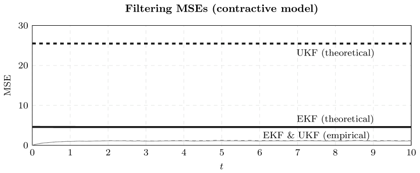
Figure 1: Empirical mean square filtering errors based on 1,000 state and measurement trajectory realisations and the theoretical error bounds (31) for the EKF and the UKF applied to the model (30). Time-averaged empirical MSEs are $1.058$ (EKF) and $1.128$ (UKF).

6.2 Integrated Velocity Model

We now validate the theoretical bounds obtained in Section 3 on the integrated velocity model discussed in Section 5.3. Consider the EKF for the integrated velocity model (28) with the parameters $a_{1}=0$, $a_{2}=1$, $q_{1}=q_{2}=0.05$, $h=1$, $r=0.05$, $\widehat{X}_{0}=0$, $\mu_{0}=0$, $P_{0}=0.01I$, and

$$g(x)=x\bigg{(}1+\frac{\sin x}{1+x^{2}}\bigg{)},\quad g^{\prime}(x)=1+\frac{(x^{3}+x)\cos x-(x^{2}-1)\sin x}{(1+x)^{2}}.$$

The maximum and minimum of $g^{\prime}$ are $\sup_{x\in\mathbb{R}}g^{\prime}(x)\approx 1.581$ and $\inf_{x\in\mathbb{R}}g^{\prime}(x)\approx 0.419$. That is, $g$ satisfies (27) with $\ell_{g}=0.419$. Based on the derivations in Section 5.3 we are able to compute that $\operatorname{tr}(P_{t})\leq\lambda_{P}\approx 0.173$ for all sufficiently large $t$. Because $a_{1}=0$, no covariance inflation is needed for (29) to hold. In this particular case, the value $\lambda=0.5478$ can be used in Theorem 3.1.

Figure 2 depicts the limiting (i.e., all exponentially decaying terms are disregarded) theoretical mean square filtering error bound for the EKF thus obtained and the empirical mean square error based on 1,000 state and measurement trajectory realisations. Again, Euler–Maruyama discretization with step-size 0.01 was used.

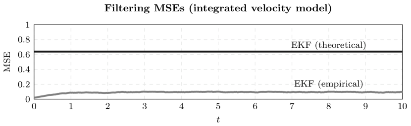
Figure 2: Empirical mean square filtering errors based on 1,000 state and measurement trajectory realisations and the limiting theoretical error bound for the EKF applied to an integrated velocity model.

7 Conclusions and Discussion

In this article we have shown that large classes of generic filters for both continuous and discrete-time systems with non-linear state dynamics and linear measurements are stable in the sense of time-uniformly bounded mean square filtering error if certain stringent conditions on boundedness of error covariance matrices and the filtering error process are met. The analysis extends the previous work [19] for the extended Kalman–Bucy filter and fully observed and exponentially stable state models. Our main contributions have been generalizations to models that need not be fully observed or exponentially stable and to a large class of commonly used extensions of the Kalman–Bucy or Kalman filter to non-linear systems, such as Gaussian assumed density filters and their numerical approximation, including the unscented Kalman filter. In Section 5, we have also presented three different classes of models and filters that satisfy the stability assumptions. This is in stark contrast to earlier work for, for example, the UKF that has relied on unverifiable assumptions on certain auxiliary random matrices [54].

The results rely on admittedly very strong conditions on the filtering error process. These conditions cannot be significantly relaxed unless a more sophisticated proof technique is devised as the technique we have used essentially neglects potential non-linear couplings of state components. It appears to us that no such technique exists at the moment. The only non-trivial and interesting extensions that we believe are possible are to fully detected systems, essentially generalizations of the integrated velocity model we considered in Section 5.3, where not all state components need to be (fully) observed, but those that are not must be exponentially stable so that their effect on observed components is small.

Appendix A Gaussian Assumed Density and Integration Filters

This appendix proves that the Gaussian assumed density and integration filters defined in Sections 2.5.2 and 2.5.3 satisfy Assumption 2.4.

For the Gaussian assumed density filter the functional $\mathcal{L}_{x,P}^{\text{\tiny{ADF}}}$ is defined in (9). For any differentiable $g\colon\mathbb{R}^{d_{x}}\to\mathbb{R}^{d_{x}}$ we have

$$\begin{split}\big{\langle}x-{\tilde{x}},g(x)-\mathcal{L}_{{\tilde{x}},P}^{\text{\tiny{ADF}}}(g)\big{\rangle}&\\ &=\big{\langle}x-{\tilde{x}},g(x)-\mathbb{E}_{\mathcal{N}({\tilde{x}},P)}(g)\big{\rangle}\\ &=\int_{\mathbb{R}^{d_{x}}}\big{\langle}(x-z)+(z-{\tilde{x}}),g(x)-g(z)\big{\rangle}\,\mathcal{N}(z\mid{\tilde{x}},P)\operatorname{d\!}z\\ &=\int_{\mathbb{R}^{d_{x}}}\big{\langle}x-z,g(x)-g(z)\big{\rangle}\,\mathcal{N}(z\mid{\tilde{x}},P)\operatorname{d\!}z-\int_{\mathbb{R}^{d_{x}}}\big{\langle}z-{\tilde{x}},g(z)\big{\rangle}\,\mathcal{N}(z\mid{\tilde{x}},P)\operatorname{d\!}z.\end{split}$$

The first term can be bounded as

$$\begin{split}\int_{\mathbb{R}^{d_{x}}}\big{\langle}x-z,g(x)-g(z)\big{\rangle}\,\mathcal{N}(z\mid{\tilde{x}},P)\operatorname{d\!}z&\\ &\leq M(g)\int_{\mathbb{R}^{d_{x}}}\mathinner{\lVert x-z\rVert}^{2}\,\mathcal{N}(z\mid{\tilde{x}},P)\operatorname{d\!}z\\ &=M(g)\bigg{(}\int_{\mathbb{R}^{d_{x}}}\big{(}\mathinner{\lVert z-{\tilde{x}}\rVert}^{2}+\mathinner{\lVert x-{\tilde{x}}\rVert}^{2}\big{)}\,\mathcal{N}(z\mid{\tilde{x}},P)\operatorname{d\!}z\bigg{)}\\ &=M(g)\big{[}\mathinner{\lVert x-{\tilde{x}}\rVert}^{2}+\operatorname{tr}(P)\big{]},\end{split}$$

whereas the second has the bound

$$\begin{split}-\int_{\mathbb{R}^{d_{x}}}\big{\langle}z-{\tilde{x}},g(z)\big{\rangle}\,\mathcal{N}(z\mid{\tilde{x}},P)\operatorname{d\!}z&=-\int_{\mathbb{R}^{d_{x}}}\big{\langle}z-{\tilde{x}},g(z)-g({\tilde{x}})\big{\rangle}\,\mathcal{N}(z\mid{\tilde{x}},P)\operatorname{d\!}z\\ &\leq-N(g)\int_{\mathbb{R}^{d_{x}}}\mathinner{\lVert z-{\tilde{x}}\rVert}^{2}\,\mathcal{N}(z\mid{\tilde{x}},P)\operatorname{d\!}z\\ &=-N(g)\operatorname{tr}(P).\end{split}$$

These estimates show that Section 2.4 holds with $C_{g}=M(g)-N(g)\geq 0$.

For the Gaussian integration filter the functional $\mathcal{L}_{x,P}^{\text{\tiny{int}}}$ is defined in (10). That (11) holds for any polynomial of total degree up to two implies that $\sum_{i=1}^{n}w_{i}=1$ and $\sum_{i=1}^{n}w_{i}\sqrt{P}\xi_{i}=0$ since $\mathcal{L}_{x,P}^{\text{\tiny{int}}}(1)=\mathcal{L}_{\mathcal{N}(x,P)}(1)=1$ and $\mathcal{L}_{x,P}^{\text{\tiny{int}}}(p)=\mathbb{E}_{\mathcal{N}(x,P)}(p)=0$ for $p(z)=z-x$. Under these assumptions we can proceed as above:

$$\big{\langle}x-\tilde{x},g(x)-\mathcal{L}_{\tilde{x},P}^{\text{\tiny{int}}}(g)\big{\rangle}={} \bigg{\langle}x-\tilde{x},g(x)-\sum_{i=1}^{n}w_{i}g\big{(}\tilde{x}+\sqrt{P}\xi_{i}\big{)}\bigg{\rangle}$$

$$={} \sum_{i=1}^{n}w_{i}\Big{\langle}x-\big{(}\tilde{x}+\sqrt{P}\xi_{i}\big{)}+\sqrt{P}\xi_{i},g(x)-g\big{(}\tilde{x}+\sqrt{P}\xi_{i}\big{)}\Big{\rangle}$$

$$={} \sum_{i=1}^{n}w_{i}\bigg{(}\Big{\langle}x-\big{(}\tilde{x}+\sqrt{P}\xi_{i}\big{)},g(x)-g\big{(}\tilde{x}+\sqrt{P}\xi_{i}\big{)}\Big{\rangle}$$

$$\quad\quad\quad\quad+\Big{\langle}\sqrt{P}\xi_{i},g(x)-g\big{(}\tilde{x}+\sqrt{P}\xi_{i}\big{)}\Big{\rangle}\bigg{)}$$

Hence

$$\begin{split}\big{\langle}x-\tilde{x},g(x)-\mathcal{L}_{\tilde{x}y,P}(g)\big{\rangle}\leq{}&M(g)\sum_{i=1}^{n}w_{i}\mathinner{\!\bigl{\lVert}x-\big{(}\tilde{x}+\sqrt{P}\xi_{i}\big{)}\bigr{\rVert}}^{2}\\ &+\sum_{i=1}^{n}w_{i}\Big{\langle}\sqrt{P}\xi_{i},g(x)-g\big{(}\tilde{x}+\sqrt{P}\xi_{i}\big{)}\Big{\rangle}.\end{split}$$

The first term is a sigma-point approximation of a quadratic function. Using (11) and proceeding again as in Section 2.5.2,

$$\sum_{i=1}^{n}w_{i}\mathinner{\!\bigl{\lVert}x-\big{(}{\tilde{x}}+\sqrt{P}\xi_{i}\big{)}\bigr{\rVert}}^{2}=\int_{\mathbb{R}^{d_{x}}}\mathinner{\lVert x-z\rVert}^{2}\,\mathcal{N}(z\mid{\tilde{x}},P)\operatorname{d\!}z=\mathinner{\lVert x-{\tilde{x}}\rVert}^{2}+\operatorname{tr}(P).$$

To bound the second term, notice that

$$\begin{split}\sum_{i=1}^{n}w_{i}&\Big{\langle}\sqrt{P}\xi_{i},g(x)-g\big{(}{\tilde{x}}+\sqrt{P}\xi_{i}\big{)}\Big{\rangle}\\ &=-\sum_{i=1}^{n}w_{i}\Big{\langle}{\tilde{x}}-\big{(}{\tilde{x}}+\sqrt{P}\xi_{i}\big{)},g({\tilde{x}})-g\big{(}{\tilde{x}}+\sqrt{P}\xi_{i}\big{)}\Big{\rangle}\\ &\leq-N(g)\sum_{i=1}^{n}\mathinner{\!\bigl{\lVert}\sqrt{P}\xi_{i}\bigr{\rVert}}^{2}\\ &=-N(g)\operatorname{tr}(P)\end{split}$$

by exactness of $\mathcal{L}_{\tilde{x},P}^{\text{\tiny{int}}}$ for quadratic polynomials. Section 2.4 thus holds with the constant $C_{g}=M(g)-N(g)$.

Appendix B Grönwall’s Inequalities

Classical Grönwall inequalities are a basic ingredients in our proofs.

Continuous version

Suppose that $\beta_{t}$ is a continuous real-valued function of $t\in\mathbb{R}$ and $x_{t}$ is continuously differentiable on $\mathbb{R}_{+}$ and satisfies $\partial_{t}x_{t}\leq\alpha x_{t}+\beta_{t}$, $t\geq 0$, for some constant $\alpha$. Then Grönwall’s inequality states that

(32) $$x_{t}\leq x_{0}\operatorname{e}^{\alpha t}+\int_{0}^{t}\operatorname{e}^{\alpha(t-s)}\beta_{s}\operatorname{d\!}s$$

for every $t\geq 0$. If $\beta_{t}\equiv\beta$, (32) reduces to

(33) $$x_{t}\leq x_{0}\operatorname{e}^{\alpha t}-(1-\operatorname{e}^{\alpha t})\beta/\alpha.$$

The form of (33) that we need the most is the one where $\beta_{t}\equiv\beta\geq 0$ and $\alpha=-\gamma$ for $\gamma>0$. Then the inequality takes the form $x_{t}\leq x_{0}\operatorname{e}^{-\gamma t}+\beta/\gamma$.

Discrete version

Let ${0\leq\alpha<1}$ and $\beta\geq 0$ and suppose that $x_{k}\geq 0$ satisfy the difference inequality $x_{k}\leq\alpha x_{k-1}+\beta$ for $k\geq 1$. Then the discrete Grönwall’s inequality states that

(34) $$x_{k}\leq\alpha^{k}x_{0}+\beta\sum_{n=0}^{k-1}\alpha^{n}\leq\alpha^{k}x_{0}+\frac{\beta}{1-\alpha}.$$

Appendix C Bernstein’s Concentration Inequality

In contrast to Del Moral et al. [19] who base their exponential concentration inequality for the EKF on the concentration inequality appearing in Proposition 11.6.6 of [17], we use a version of the classical Bernstein inequality.

Theorem C.1 (Bernstein’s inequality).

Let $X$ be a non-negative random variable. Suppose that there is $\alpha>0$ such that $\mathbb{E}(X^{n})\leq n^{n}\alpha^{n}$ for every integer $n\geq 2$. Then

(35) $$\mathbb{P}\big{[}X\geq\alpha\operatorname{e}\big{(}\sqrt{2\delta}+\delta\big{)}\big{]}\leq\operatorname{e}^{-\delta}$$

for any $\delta>0$.

Proof C.2.

By the standard Stirling bound,

$$\mathbb{E}(X^{n})\leq n^{n}\alpha^{n}\leq\frac{n!}{\sqrt{2\pi}}\operatorname{e}^{n}\alpha^{n}\leq\frac{n!}{2}(\operatorname{e}\alpha)^{n}$$

for every $n\geq 2$. The “standard” version of Bernstein’s inequality (e.g., [10, Theorem 2.10]) posits that $\mathbb{E}(X^{2})\leq\sigma<\infty$ and $\mathbb{E}(X^{n})\leq\frac{n!}{2}\sigma\gamma^{n-2}$ for some $\sigma>0$ and $\gamma>0$ and every $n\geq 3$ imply $\mathbb{P}[X\geq\sqrt{2\sigma\delta}+\gamma\delta]\leq\operatorname{e}^{-\delta}$ for any $\delta>0$. Thus, setting $\gamma=\operatorname{e}\alpha$ and $\sigma=\gamma^{2}$ produces the claim.

The concentration inequality used in [19, Equation (3.6)] is based on the same moment bounds $\mathbb{E}(X^{n})\leq n^{n}\alpha^{n}$ but states instead that

$$\mathbb{P}\,\bigg{[}X\geq\frac{\alpha\operatorname{e}^{2}}{\sqrt{2}}\bigg{(}\frac{1}{2}+\sqrt{\delta}+\delta\bigg{)}\bigg{]}\leq\operatorname{e}^{-\delta}$$

for any $\delta>0$. Since

$$\mathbb{P}\big{[}X\geq\alpha\operatorname{e}\big{(}\sqrt{2\delta}+\delta\big{)}\big{]}=\mathbb{P}\bigg{[}X\geq\alpha\sqrt{2}\operatorname{e}\bigg{(}\sqrt{\delta}+\frac{1}{\sqrt{2}}\delta\bigg{)}\bigg{]}$$

and $\sqrt{2}\operatorname{e}<\operatorname{e}^{2}/\sqrt{2}$, the inequality (35) is the tighter of the two for every $\delta>0$.

Lemma C.3.

Let $X\sim\mathcal{N}(m,P)$ be a $d$-dimensional Gaussian random vector with a positive-semidefinite covariance $P$. Then

$$\mathbb{E}(\mathinner{\lVert X\rVert}^{2n})^{1/n}\leq 4\big{(}\mathinner{\lVert m\rVert}^{2}+\mathinner{\lVert P\rVert}[d+2]n\big{)}$$

for every $n\in\mathbb{N}$. If $m=0$, the inequality is

$$\mathbb{E}(\mathinner{\lVert X\rVert}^{2n})^{1/n}\leq\mathinner{\lVert P\rVert}(d+2)n.$$

Proof C.4.

We know that $X=m+P^{1/2}U$ for a standard normal $U\in\mathbb{R}^{d}$. Therefore

$$\begin{split}\mathbb{E}(\mathinner{\lVert X\rVert}^{2n})=\mathbb{E}\big{(}\big{[}\mathinner{\lVert m\rVert}+\mathinner{\lVert P^{1/2}U\rVert}\big{]}^{2n}\big{)}&\leq 2^{2n-1}\big{(}\mathinner{\lVert m\rVert}^{2n}+\mathbb{E}\big{[}(U^{\mathsf{T}}PU)^{n}\big{]}\big{)}\\ &\leq 2^{2n-1}\big{(}\mathinner{\lVert m\rVert}^{2n}+\mathinner{\lVert P\rVert}^{n}\mathbb{E}[\mathinner{\lVert U\rVert}^{2n}]\big{)},\end{split}$$

where $\mathbb{E}(\mathinner{\lVert U\rVert}^{2n})$ is the $n$th moment around zero of the chi-squared distribution with degrees of freedom $d$. That is,

$$\mathbb{E}(\mathinner{\lVert U\rVert}^{2n})=d\times\cdots\times(d+2(n-1))\leq(d+2(n-1))^{n}\leq(d+2)^{n}n^{n}.$$

The inequality $(a+b)^{1/n}\leq a^{1/n}+b^{1/n}$ for any $a,b>0$ yields the first claim. The second claim follows from $\mathbb{E}(\mathinner{\lVert X\rVert}^{2n})=\mathbb{E}([U^{\mathsf{T}}PU]^{n})$ if $X$ is zero-mean.

Appendix D Proof of Theorem 3.1

This appendix contains the complete proof of Theorem 3.1. We begin with a proposition providing bounds for functions satisfying certain differential inequalities. This proposition is a modification of Grönwall’s inequalities (32) and (33) and appears also in [19, Appendix A.2].

Proposition D.1.

Let $\alpha\neq 0$ and $\beta\geq 0$ be constants and $n$ a positive integer. Suppose that a non-negative and differentiable function $x_{t}$ satisfies the differential inequality $\partial_{t}x_{t}\leq\alpha nx_{t}+\beta n^{2}x_{t}^{1-1/n}$ for $t\geq t_{0}$. Then

$$x_{t}^{1/n}\leq x_{t_{0}}^{1/n}\operatorname{e}^{\alpha(t-t_{0})}+\frac{\beta n}{\alpha}\big{(}\operatorname{e}^{\alpha(t-t_{0})}-1\big{)}.$$

Proof D.2.

For $t\geq t_{0}$, the function $z_{t}=\operatorname{e}^{-\alpha n(t-t_{0})}x_{t}\geq 0$ satisfies

$$\partial_{t}z_{t}=-\alpha n\operatorname{e}^{-\alpha n(t-t_{0})}x_{t}+\operatorname{e}^{-\alpha n(t-t_{0})}\partial_{t}x_{t} \leq n^{2}\beta\operatorname{e}^{-\alpha n(t-t_{0})}x_{t}^{1-1/n}$$

$$=\beta n^{2}\operatorname{e}^{-\alpha(t-t_{0})}z_{t}^{1-1/n}.$$

Consequently, for $t\geq t_{0}$, $\partial_{t}z_{t}^{1/n}=n^{-1}z_{t}^{1/n-1}\partial_{t}z_{t}\leq\beta n\operatorname{e}^{-\alpha(t-t_{0})}$ and direct integration yields

$$z_{t}^{1/n}\leq z_{t_{0}}^{1/n}+\beta n\int_{t_{0}}^{t}\operatorname{e}^{-\alpha(s-t_{0})}\operatorname{d\!}s=z_{t_{0}}^{1/n}+\frac{\beta n}{\alpha}\big{(}1-\operatorname{e}^{-\alpha(t-t_{0})}\big{)}.$$

The claim is obtained by observing that $x^{1/n}_{t}=\operatorname{e}^{\alpha(t-t_{0})}z^{1/n}_{t}$.

Proof D.3 (Proof of Theorem 3.1).

Application of Itô’s lemma to (12) yields

$$\begin{split}\operatorname{d\!}\mathinner{\lVert E_{t}\rVert}^{2}={}&\operatorname{d\!}M_{t}+\big{[}\operatorname{tr}(Q)+\operatorname{tr}(SP_{t}^{2})\big{]}\operatorname{d\!}t\\ &+2\big{\langle}f(X_{t})-\mathcal{L}_{\widehat{X}_{t},P_{t}}(f)-P_{t}S(X_{t}-\widehat{X}_{t}),X_{t}-\widehat{X}_{t}\big{\rangle}\operatorname{d\!}t,\end{split}$$

where

$$\operatorname{d\!}M_{t}=2\big{\langle}Q^{1/2}\operatorname{d\!}W_{t}-P_{t}H^{\mathsf{T}}R^{-1/2}\operatorname{d\!}V_{t},X_{t}-\widehat{X}_{t}\big{\rangle}$$

is a zero-mean (local) martingale. Keeping in mind that ${\mathcal{L}_{\widehat{X}_{t},P_{t}}(A)=A\widehat{X}_{t}}$ for any $A\in\mathbb{R}^{d_{x}\times d_{x}}$, we write

$$f(X_{t})-\mathcal{L}_{\widehat{X}_{t},P_{t}}(f)-P_{t}S(X_{t}-\widehat{X}_{t})=f(X_{t})-P_{t}SX_{t}-\mathcal{L}_{\widehat{X}_{t},P_{t}}\big{(}f-P_{t}S\big{)}$$

and apply Section 2.4 to the function $g=f-P_{t}S$ with $x=X_{t}$ and $\tilde{x}=\widehat{X}_{t}$:

$$\big{\langle}f(X_{t})-\mathcal{L}_{\widehat{X}_{t},P_{t}}(f)-P_{t}S(X_{t}-\widehat{X}_{t}),X_{t}-\widehat{X}_{t}\big{\rangle}\leq-\lambda\mathinner{\lVert X_{t}-\widehat{X}_{t}\rVert}^{2}+C_{\lambda}\operatorname{tr}(P_{t}),$$

where $C_{\lambda}\geq 0$ is finite because $M(f-P_{t}S)\leq-\lambda$ and

$$\begin{split}N(f-P_{t}S)\geq N(f)+\nu(-P_{t}S)=N(f)-\mu(P_{t}S)&\geq N(f)-\mathinner{\lVert P_{t}\rVert}\mathinner{\lVert S\rVert}\\ &\geq N(f)-\operatorname{tr}(S)\lambda_{P},\end{split}$$

which is finite by (4) and the assumption $\sup_{t\geq 0}\operatorname{tr}(P_{t})\leq\lambda_{P}$. For $t\geq T$, the assumption (13), together with (2), produces the almost sure bound

$$\operatorname{d\!}\mathinner{\lVert E_{t}\rVert}^{2}\leq-2\lambda\mathinner{\lVert E_{t}\rVert}^{2}\operatorname{d\!}t+u\operatorname{d\!}t+\operatorname{d\!}M_{t},$$

where $u=\operatorname{tr}(Q)+2C_{\lambda}\lambda_{P}+\operatorname{tr}(S)\lambda_{P}^{2}$. Taking expectations and using Grönwall’s inequality then yield the claimed mean square bound

(36) $$\mathbb{E}(\mathinner{\lVert E_{t}\rVert}^{2})\leq\mathbb{E}(\mathinner{\lVert E_{T}\rVert}^{2})\operatorname{e}^{-2\lambda(t-T)}+u/(2\lambda),$$

with $\mathbb{E}(\mathinner{\lVert E_{T}\rVert}^{2})$ being finite due to finiteness of $N(f)$ and $M(f)$. This concludes the proof of (15).

To prove the exponential concentration inequality (14) we compute upper bounds on $\mathbb{E}(\mathinner{\lVert E_{t}\rVert}^{2n})$ for every $n\geq 1$ in order to use Theorem C.1. First, note that for $0\leq t\leq T$ we have the inequality $\operatorname{d\!}\mathinner{\lVert E_{t}\rVert}^{2}\leq 2\rho\mathinner{\lVert E_{t}\rVert}^{2}\operatorname{d\!}t+u\operatorname{d\!}t+\operatorname{d\!}M_{t}$, where

$$\rho=M(f)+\mathinner{\lVert S\rVert}\operatorname{tr}(P_{t})\geq M(f)+\mu(-P_{t}S)\geq M(f-P_{t}S).$$

In the following we can assume that $\rho>0$, for if it were negative we could set $-\lambda=\rho$ and $T=0$. Let $\gamma$ stand for either $-\lambda$ or $\rho$. Observe that $\langle M\rangle_{t}$, the quadratic variation of $M_{t}$ (the increasing process such that $M_{t}^{2}-\langle M\rangle_{t}$ is a martingale), satisfies

$$\operatorname{d\!}\,\langle M\rangle_{t}\leq 4\mathinner{\lVert E_{t}\rVert}^{2}\big{[}\operatorname{tr}(Q)+\operatorname{tr}(SP_{t}^{2})\big{]}\operatorname{d\!}t\leq 4\mathinner{\lVert E_{t}\rVert}^{2}u\operatorname{d\!}t.$$

For $n\geq 2$, the above inequality, the identity ${\operatorname{d\!}\,\langle\mathinner{\lVert E\rVert}^{2}\rangle_{t}=\operatorname{d\!}\,\langle M\rangle_{t}}$, and the general form of Itô’s lemma then produce

$$\begin{split}\operatorname{d\!}\mathinner{\lVert E_{t}\rVert}^{2n}={}&n\mathinner{\lVert E_{t}\rVert}^{2(n-1)}\operatorname{d\!}\mathinner{\lVert E_{t}\rVert}^{2}+\frac{n(n-1)}{2}\mathinner{\lVert E_{t}\rVert}^{2(n-2)}\operatorname{d\!}\,\langle\mathinner{\lVert E\rVert}^{2}\rangle_{t}\\ ={}&n\mathinner{\lVert E_{t}\rVert}^{2(n-1)}\operatorname{d\!}\mathinner{\lVert E_{t}\rVert}^{2}+\frac{n(n-1)}{2}\mathinner{\lVert E_{t}\rVert}^{2(n-2)}\operatorname{d\!}\,\langle M\rangle_{t}\\ \leq{}&2\gamma n\mathinner{\lVert E_{t}\rVert}^{2n}\operatorname{d\!}t+2un^{2}\mathinner{\lVert E_{t}\rVert}^{2(n-1)}\operatorname{d\!}t+n\mathinner{\lVert E_{t}\rVert}^{2(n-1)}\operatorname{d\!}M_{t}.\end{split}$$

Induction establishes that $\mathbb{E}(\mathinner{\lVert E_{t}\rVert}^{2n})$ does not explode in finite time. Thus the term $\mathinner{\lVert E_{t}\rVert}^{2(n-1)}\operatorname{d\!}M_{t}$ vanishes when expectations are taken (see, e.g., [29, Section 4.5] for similar arguments). Using Hölder’s inequality with $p=n/(n-1)$, we get

$$\begin{split}\partial_{t}\mathbb{E}(\mathinner{\lVert E_{t}\rVert}^{2n})&\leq 2\gamma n\,\mathbb{E}(\mathinner{\lVert E_{t}\rVert}^{2n})+2un^{2}\,\mathbb{E}(\mathinner{\lVert E_{t}\rVert}^{2(n-1)})\\ &\leq 2\gamma n\mathbb{E}(\mathinner{\lVert E_{t}\rVert}^{2n})+2un^{2}\mathbb{E}(\mathinner{\lVert E_{t}\rVert}^{2n})^{1-1/n}.\end{split}$$

We can now apply Proposition D.1 with $x_{t}=\mathinner{\lVert E_{t}\rVert}^{2n}$ and $\beta=u$. Setting $\alpha=2\rho$ and $t_{0}=0$ and considering $t\leq T$, we obtain

$$\mathbb{E}(\mathinner{\lVert E_{T}\rVert}^{2n})^{1/n}\leq\bigg{[}\mathbb{E}(\mathinner{\lVert E_{0}\rVert}^{2n})^{1/n}+\frac{un}{2\rho}\bigg{]}\operatorname{e}^{2\rho T}.$$

Recall that $X_{0}\sim\mathcal{N}(\mu_{0},\Sigma_{0})$ and $\widehat{X}_{0}=\hat{x}_{0}$ is deterministic. Thus $E_{0}\sim\mathcal{N}(\mu_{0}-\hat{x}_{0},\Sigma_{0})$ so that Lemma C.3 gives

$$\begin{split}\mathbb{E}(\mathinner{\lVert E_{T}\rVert}^{2n})^{1/n}&\leq\bigg{[}4\big{(}\mathinner{\lVert\mu_{0}-\hat{x}_{0}\rVert}^{2}+\mathinner{\lVert P_{0}\rVert}[d_{x}+2]n\big{)}+\frac{un}{2\rho}\bigg{]}\operatorname{e}^{2\rho T}\\ &\leq\underbrace{4\bigg{[}\mathinner{\lVert\mu_{0}-\hat{x}_{0}\rVert}^{2}+\mathinner{\lVert P_{0}\rVert}(d_{x}+2)+\frac{un}{8\rho}\bigg{]}\operatorname{e}^{2\rho T}}_{\eqqcolon C_{T}}n.\end{split}$$

This provides a bound on the initial value for the case $\alpha=-2\lambda$, $t_{0}=T$, and $t\geq T$ in Proposition D.1:

$$\mathbb{E}(\mathinner{\lVert E_{t}\rVert}^{2n})^{1/n}\leq\mathbb{E}(\mathinner{\lVert E_{T}\rVert}^{2n})^{1/n}\operatorname{e}^{-2\lambda(t-T)}+\frac{un}{2\lambda}\leq\bigg{(}C_{T}\operatorname{e}^{-2\lambda(t-T)}+\frac{u}{2\lambda}\bigg{)}n.$$

That is,

$$\mathbb{E}(\mathinner{\lVert E_{t}\rVert}^{2n})\leq\Big{(}C_{T}\operatorname{e}^{-2\lambda(t-T)}+u/(2\lambda)\Big{)}^{n}n^{n}.$$

The claimed exponential concentration inequality follows by applying Bernstein’s inequality of Theorem C.1 to $X=\mathinner{\lVert E_{t}\rVert}^{2}$ with $\alpha=C_{T}\operatorname{e}^{-2\lambda(t-T)}+u/(2\lambda)$.

Appendix E Proof of Theorem 4.2

Proof E.1 (Proof of Theorem 4.2).

Norm of the filtering error is

$$\begin{split}\mathinner{\lVert E_{k}\rVert}^{2}={}&\big{[}f(X_{k-1})-\mathcal{L}_{\widehat{X}_{k-1},P_{k-1}}(f)\big{]}^{\mathsf{T}}(I-K_{k}H)^{\mathsf{T}}\\ &\quad\quad\times(I-K_{k}H)\big{[}f(X_{k-1})-\mathcal{L}_{\widehat{X}_{k-1},P_{k-1}}(f)\big{]}\\ &+2\big{[}f(X_{k-1})-\mathcal{L}_{\widehat{X}_{k-1},P_{k-1}}(f)\big{]}^{\mathsf{T}}(I-K_{k}H)^{\mathsf{T}}\\ &\quad\quad\times\big{[}(I-K_{k}H)Q^{1/2}W_{k}-K_{k}R^{1/2}V_{k}\big{]}\\ &+\big{[}(I-K_{k}H)Q^{1/2}W_{k}-K_{k}R^{1/2}V_{k}\big{]}^{\mathsf{T}}\big{[}(I-K_{k}H)Q^{1/2}W_{k}-K_{k}R^{1/2}V_{k}\big{]}.\end{split}$$

We immediately obtain

$$\kappa=\sup_{k\geq 1}\mathinner{\lVert K_{k}\rVert}=\mathinner{\!\bigl{\lVert}P_{k\mid k-1}H^{\mathsf{T}}(HP_{k\mid k-1}H^{\mathsf{T}}+R)^{-1}\bigr{\rVert}}\leq\lambda_{P}^{p}\mathinner{\lVert H\rVert}\mathinner{\lVert R^{-1}\rVert}.$$

Using Assumption 4.1 and (20), we get the recursive filtering error bound

(37) $$\mathinner{\lVert E_{k}\rVert}^{2}\leq\lambda_{df}^{2}\mathinner{\lVert E_{k-1}\rVert}^{2}+C_{f}\lambda_{d}^{2}\lambda_{P}^{u}+\mathinner{\lVert U_{k}\rVert}^{2}+2M_{k},$$

where $C_{f}$ is the constant of Assumption 4.1 for the function $f$ and the random variables

$$U_{k}=(I-K_{k}H)Q^{1/2}W_{k}-K_{k}R^{1/2}V_{k}$$

and

$$M_{k}=\big{[}f(X_{k-1})-\mathcal{L}_{\widehat{X}_{k-1},P_{k-1}}(f)\big{]}^{\mathsf{T}}(I-K_{k}H)^{\mathsf{T}}U_{k}$$

are zero-mean because $W_{k}$ and $V_{k}$ are independent of $X_{k-1}$, $\widehat{X}_{k-1}$, $P_{k-1}$, and $K_{k}$. Because

(38) $$\mathbb{E}(\mathinner{\lVert U_{k}\rVert}^{2})\leq u_{d}\coloneqq\lambda_{d}^{2}\operatorname{tr}(Q)+\kappa^{2}\operatorname{tr}(R),$$

we have

$$\mathbb{E}(\mathinner{\lVert E_{k}\rVert}^{2})\leq\lambda_{df}^{2}\mathbb{E}(\mathinner{\lVert E_{k-1}\rVert}^{2})+u_{d}+C_{f}\lambda_{d}^{2}\lambda_{P}^{u}.$$

The discrete Grönwall’s inequality (34) then produces

$$\mathbb{E}(\mathinner{\lVert E_{k}\rVert}^{2})\leq\lambda_{df}^{2k}\mathbb{E}(\mathinner{\lVert E_{0}\rVert}^{2})+\frac{u_{d}+C_{f}\lambda_{d}^{2}\lambda_{P}^{u}}{1-\lambda_{df}^{2}}=\lambda_{df}^{2k}\big{(}\mathinner{\lVert\mu_{0}-\hat{x}_{0}\rVert}^{2}+\operatorname{tr}(\Sigma_{0})\big{)}+\frac{u_{d}+C_{f}\lambda_{d}^{2}\lambda_{P}^{u}}{1-\lambda_{df}^{2}},$$

which is the mean square bound (22). Here we have used $\mathbb{E}(\mathinner{\lVert X\rVert}^{2})=\operatorname{tr}(P)+\mathinner{\lVert m\rVert}^{2}$, which holds for any Gaussian random vector $X\sim\mathcal{N}(m,P)$.

To obtain the concentration inequality (21), we bound $\mathbb{E}(\mathinner{\lVert E_{k}\rVert}^{2n})$ for every $n\geq 1$ and use Bernstein’s inequality. The random variable $M_{k}$ admits the bound

$$M_{k}\leq\big{(}\lambda_{df}\mathinner{\lVert E_{k-1}\rVert}+\eta\big{)}\mathinner{\lVert U_{k}\rVert}\quad\text{ with }\quad\eta=\lambda_{d}(C_{f}\lambda_{P}^{u})^{1/2}.$$

Inequality (37) gives

$$\mathbb{E}(\mathinner{\lVert E_{k}\rVert}^{2n})\leq\mathbb{E}\big{[}\big{(}\lambda_{df}^{2}\mathinner{\lVert E_{k-1}\rVert}^{2}+\mathinner{\lVert U_{k}\rVert}^{2}+2M_{k}+\eta^{2}\big{)}^{n}\big{]}$$

and consequently Minkowski’s inequality yields

(39) $$\begin{split}\mathbb{E}(\mathinner{\lVert E_{k}\rVert}^{2n})^{1/n}&\leq\mathbb{E}\big{[}\big{(}\lambda_{df}^{2}\mathinner{\lVert E_{k-1}\rVert}^{2}+\mathinner{\lVert U_{k}\rVert}^{2}+2M_{k}+\eta^{2}\big{)}^{n}\big{]}^{1/n}\\ &\leq\lambda_{df}^{2}\mathbb{E}(\mathinner{\lVert E_{k-1}\rVert}^{2n})^{1/n}+\mathbb{E}(\mathinner{\lVert U_{k}\rVert}^{2n})^{1/n}+2\mathbb{E}(M_{k}^{n})^{1/n}+\eta^{2}.\end{split}$$

By Lemma C.3 and (38), $\mathbb{E}(\mathinner{\lVert U_{k}\rVert}^{2n})^{1/n}\leq(d_{x}+2)nu_{d}$, and by Minkowski’s and Hölder’s inequalities,

$$\begin{split}\mathbb{E}(M_{k}^{n})^{1/n}&\leq\mathbb{E}(\mathinner{\lVert U_{k}\rVert}^{n})^{1/n}\mathbb{E}\big{(}[\lambda_{df}\mathinner{\lVert E_{k-1}\rVert}+\eta]^{n}\big{)}^{1/n}\\ &\leq\mathbb{E}(\mathinner{\lVert U_{k}\rVert}^{n})^{1/n}\big{[}\lambda_{df}\mathbb{E}(\mathinner{\lVert E_{k-1}\rVert}^{n})^{1/n}+\eta\big{]}\\ &\leq\mathbb{E}(\mathinner{\lVert U_{k}\rVert}^{2n})^{1/(2n)}\big{[}\lambda_{df}\mathbb{E}(\mathinner{\lVert E_{k-1}\rVert}^{2n})^{1/(2n)}+\eta\big{]}\\ &\leq\sqrt{(d_{x}+2)nu_{d}}\big{[}\lambda_{df}\mathbb{E}(\mathinner{\lVert E_{k-1}\rVert}^{2n})^{1/(2n)}+\eta\big{]}.\end{split}$$

Inserting these bounds into (39) and recognizing that the result can be bounded by a sum of two quadratic terms produces

$$\mathbb{E}(\mathinner{\lVert E_{k}\rVert}^{2n})^{1/(2n)}\leq\lambda_{df}\mathbb{E}(\mathinner{\lVert E_{k-1}\rVert}^{2n})^{1/(2n)}+2\sqrt{(d_{x}+2)nu_{d}}+\eta.$$

Then the discrete Grönwall’s inequality and Lemma C.3 yield

$$\begin{split}\mathbb{E}(\mathinner{\lVert E_{k}\rVert}^{2n})^{1/(2n)}&\leq\lambda_{df}^{k}\mathbb{E}(\mathinner{\lVert E_{0}\rVert}^{2n})^{1/(2n)}+\frac{2\sqrt{(d_{x}+2)nu_{d}}+\eta}{1-\lambda_{df}}\\ &\leq\bigg{(}2\lambda_{df}^{k}\Big{[}\mathinner{\lVert\mu_{0}-\hat{x}_{0}\rVert}+\mathinner{\lVert\Sigma_{0}\rVert}^{1/2}\sqrt{(d_{x}+2)n}\,\Big{]}+\frac{2\sqrt{(d_{x}+2)nu_{d}}+\eta}{1-\lambda_{df}}\bigg{)}\\ &\leq 2\bigg{(}\lambda_{df}^{k}\Big{[}\mathinner{\lVert\mu_{0}-\hat{x}_{0}\rVert}+\mathinner{\lVert\Sigma_{0}\rVert}^{1/2}\Big{]}+\frac{\sqrt{u_{d}}+\eta}{1-\lambda_{df}}\bigg{)}\sqrt{(d_{x}+2)n}.\end{split}$$

This proves that

$$\begin{split}\mathbb{E}(\mathinner{\lVert E_{k}\rVert}^{2n})&\leq 2^{2n}\bigg{(}\lambda_{df}^{k}\Big{[}\mathinner{\lVert\mu_{0}-\hat{x}_{0}\rVert}+\mathinner{\lVert\Sigma_{0}\rVert}^{1/2}\Big{]}+\frac{\sqrt{u_{d}}+\eta}{1-\lambda_{df}}\bigg{)}^{2n}(d_{x}+2)^{n}n^{n}\end{split}$$

The claim follows from Bernstein’s inequality with $X=\mathinner{\lVert E_{k}\rVert}^{2}$ and

$$\alpha=4\bigg{(}\lambda_{df}^{k}\Big{[}\mathinner{\lVert\mu_{0}-\hat{x}_{0}\rVert}+\mathinner{\lVert\Sigma_{0}\rVert}^{1/2}\Big{]}+\frac{\sqrt{u_{d}}+\eta}{1-\lambda_{df}}\bigg{)}^{2}.$$

References

- [1] B. D. O. Anderson and J. B. Moore, Detectability and stabilizability of time-varying discrete-time linear systems, SIAM Journal on Control and Optimization, 19 (1981), pp. 20–32.
- [2] R. Atar and O. Zeitouni, Exponential stability for nonlinear filtering, Annales de l’Institut Henri Poincare (B) Probability and Statistics, 33 (1997), pp. 697–725.
- [3] J. S. Baras, A. Bensoussan, and M. R. James, Dynamic observers as asymptotic limits of recursive filters: Special cases, SIAM Journal on Applied Mathematics, 48 (1988), pp. 1147–1158.
- [4] A. Barrau and S. Bonnabel, The invariant extended Kalman filter as a stable observer, IEEE Transactions on Automatic Control, 62 (2017), pp. 1797–1812.
- [5] D. S. Bernstein, Matrix Mathematics: Theory, Facts, and Formulas, Princeton University Press, 2nd ed., 2009.
- [6] A. N. Bishop and P. Del Moral, On the stability of Kalman–Bucy diffusion processes, SIAM Journal on Control and Optimization, 55 (2017), pp. 4015–4047.
- [7] A. N. Bishop and P. Jensfelt, A stochastically stable solution to the problem of robocentric mapping, in 2009 IEEE International Conference on Robotics and Automation, 2009, pp. 1615–1622.
- [8] S. Bolognani, L. Tubiana, and M. Zigliotto, Extended Kalman filter tuning in sensorless PMSM drives, IEEE Transactions on Industry Applications, 39 (2003), pp. 1741–1747.
- [9] S. Bonnabel and J.-J. Slotine, A contraction theory-based analysis of the stability of the deterministic extended Kalman filter, IEEE Transactions on Automatic Control, 60 (2015), pp. 565–569.
- [10] S. Boucheron, G. Lugosi, and P. Massart, Concentration Inequalities: A Nonasymptotic Theory of Independence, Oxford University Press, 2013.
- [11] M. Boutayeb, H. Rafaralahy, and M. Darouach, Convergence analysis of the extended Kalman filter used as an observer for nonlinear deterministic discrete-time systems, IEEE Transactions on Automatic Control, 42 (1997), pp. 581–586.
- [12] R. S. Bucy, Global theory of the Riccati equation, Journal of Computer and System Sciences, 1 (1967), pp. 349–361.
- [13] A. Budhiraja and D. Ocone, Exponential stability in discrete-time filtering for non-ergodic signals, Stochastic Processes and their Applications, 82 (1999), pp. 245–257.
- [14] F. M. Callier and J. Winkin, Convergence of the time-invariant Riccati differential equation towards its strong solution for stabilizable systems, Journal of Mathematical Analysis and Applications, 192 (1995), pp. 230–257.
- [15] G. De Nicolao and M. Gevers, Difference and differential Riccati equations: a note on the convergence to the strong solution, IEEE Transactions on Automatic Control, 37 (1992), pp. 1055–1057.
- [16] J. de Wiljes, S. Reich, and W. Stannat, Long-time stability and accuracy of the ensemble Kalman-Bucy filter for fully observed processes and small measurement noise, SIAM Journal on Applied Dynamical Systems, 17 (2018), pp. 1152–1181.
- [17] P. Del Moral, Mean Field Simulation for Monte Carlo Integration, no. 153 in Chapman & Hall/CRC Monographs on Statistics & Applied Probability, Chapman and Hall/CRC, 1st ed., 2013.
- [18] P. Del Moral, A. Kurtzmann, and J. Tugaut, On the stability and the uniform propagation of chaos of a class of extended ensemble Kalman–Bucy filters, SIAM Journal on Control and Optimization, 55 (2017), pp. 119–155.
- [19] P. Del Moral, A. Kurtzmann, and J. Tugaut, On the stability and the concentration of extended Kalman-Bucy filters, Electronic Journal of Probability, 23 (2018).
- [20] P. Del Moral and J. Tugaut, On the stability and the uniform propagation of chaos properties of ensemble Kalman–Bucy filters, The Annals of Applied Probability, 28 (2018), pp. 790–850.
- [21] B. Delyon, A note on uniform observability, IEEE Transactions on Automatic Control, 46 (2001), pp. 1326–1327.
- [22] J. J. Deyst, Jr. and C. F. Price, Conditions for asymptotic stability of the discrete minimum-variance linear estimator, IEEE Transactions on Automatic Control, 13 (1968), pp. 702–705.
- [23] K. Ito and K. Xiong, Gaussian filters for nonlinear filtering problems, IEEE Transactions on Automatic Control, 45 (2000), pp. 910–927.
- [24] A. H. Jazwinski, Stochastic Processes and Filtering Theory, Academic Press, 1970.
- [25] S. J. Julier and J. K. Uhlmann, New extension of the Kalman filter to nonlinear systems, in Signal Processing, Sensor Fusion, and Target Recognition VI, vol. 3068, 1997, pp. 182–194.
- [26] T. Karvonen, S. Bonnabel, E. Moulines, and S. Särkkä, Bounds on the error covariance of a class of Kalman–Bucy filters for systems with non-linear dynamics, in 57th IEEE Conference on Decision and Control, 2018, pp. 7176–7181.
- [27] T. Karvonen and S. Särkkä, Fourier–Hermite series for stochastic stability analysis of non-linear Kalman filters, in 19th International Conference on Information Fusion, 2016, pp. 1829–1836.
- [28] D. T. B. Kelly, K. J. H. Law, and A. M. Stuart, Well-posedness and accuracy of the ensemble Kalman filter in discrete and continuous time, Nonlinearity, 27 (2014), pp. 2579–2603.
- [29] P. E. Kloeden and E. Platen, Numerical Solution of Stochastic Differential Equations, no. 23 in Stochastic Modelling and Applied Probability, Springer-Verlag Berlin Heidelberg, 1st ed., 1992.
- [30] S. Kluge, K. Reif, and M. Brokate, Stochastic stability of the extended Kalman filter with intermittent observations, IEEE Transactions on Automatic Control, 55 (2010), pp. 514–518.
- [31] A. J. Krener, The Convergence of the Extended Kalman Filter, vol. 286 of Lecture Notes in Control and Information Sciences, 2003, pp. 173–182.
- [32] E. Köksal Babacan, L. Özbek, and M. Efe, Stability of the extended Kalman filter when the states are constrained, IEEE Transactions on Automatic Control, 53 (2008), pp. 2707–2711.
- [33] L. Li and Y. Xia, Stochastic stability of the unscented Kalman filter with intermittent observations, Automatica, 48 (2012), pp. 978–981.
- [34] J. P. Maree, L. Imsland, and J. Jouffroy, On convergence of the unscented Kalman–Bucy filter using contraction theory, International Journal of Systems Science, 47 (2016), pp. 1816–1827.
- [35] J. Prüher and O. Straka, Gaussian process quadrature moment transform, IEEE Transactions on Automatic Control, 63 (2018), pp. 2844–2854.
- [36] K. Rapp, Nonlinear Estimation and Control in the Iron Ore Pelletizing Process: An Application and Analysis of the Extended Kalman Filter, PhD thesis, Norwegian University of Science and Technology, 2004.
- [37] K. Reif, S. Günther, E. Yaz, and R. Unbehauen, Stochastic stability of the discrete-time extended Kalman filter, IEEE Transactions on Automatic Control, 44 (1999), pp. 714–728.
- [38] K. Reif, S. Günther, E. Yaz, and R. Unbehauen, Stochastic stability of the continuous-time extended Kalman filter, IEE Proceedings - Control Theory and Applications, 147 (2000), pp. 45–52.
- [39] K. Reif, F. Sonnemann, and R. Unbehauen, Modification of the extended Kalman filter with an additive term of instability, in Proceedings of the 35th IEEE Conference on Decision and Control, vol. 4, 1996, pp. 4058–4059.
- [40] K. Reif, F. Sonnemann, and R. Unbehauen, An EKF-based nonlinear observer with a prescribed degree of stability, Automatica, 34 (1998), pp. 1119–1123.
- [41] K. Reif and R. Unbehauen, The extended Kalman filter as an exponential observer for nonlinear systems, IEEE Transactions on Signal Processing, 47 (1999), pp. 2324–2328.
- [42] T. Strom, On logarithmic norms, SIAM Journal on Numerical Analysis, 12 (1975), pp. 741–753.
- [43] S. Särkkä, On unscented Kalman filtering for state estimation of continuous-time nonlinear systems, IEEE Transactions on Automatic Control, 52 (2007), pp. 1631–1641.
- [44] S. Särkkä, Bayesian Filtering and Smoothing, Institute of Mathematical Statistics Textbooks, Cambridge University Press, 2013.
- [45] S. Särkkä, J. Hartikainen, L. Svensson, and F. Sandblom, On the relation between Gaussian process quadratures and sigma-point methods, Journal of Advances in Information Fusion, 11 (2016), pp. 31–46.
- [46] S. Särkkä and J. Sarmavuori, Gaussian filtering and smoothing for continuous-discrete dynamic systems, Signal Processing, 93 (2013), pp. 500–510.
- [47] G. Söderlind, The logarithmic norm. History and modern theory, BIT Numerical Mathematics, 46 (2006), pp. 631–652.
- [48] X. T. Tong, A. J. Majda, and D. Kelly, Nonlinear stability and ergodicity of ensemble based Kalman filters, Nonlinearity, 29 (2016), pp. 657–691.
- [49] W. M. Wonham, On a matrix Riccati equation of stochastic control, SIAM Journal on Control, 6 (1968), pp. 681–697.
- [50] Y. Wu, D. Hu, and X. Hu, Comments on “Performance evaluation of UKF-based nonlinear filtering”, Automatica, 43 (2007), pp. 567–568.
- [51] Y. Wu, D. Hu, M. Wu, and X. Hu, A numerical-integration perspective on Gaussian filters, IEEE Transactions on Automatic Control, 54 (2006), pp. 2910–2921.
- [52] K. Xiong, C. W. Chan, and H. Zhang, Detection of satellite attitude sensor faults using the UKF, IEEE Transactions on Aerospace and Electronic Systems, 43 (2007), pp. 480–491.
- [53] K. Xiong, L. D. Liu, and H. Zhang, Modified unscented Kalman filtering and its application in autonomous satellite navigation, Aerospace Science and Technology, 13 (2009), pp. 238–246.
- [54] K. Xiong, H. Zhang, and C. W. Chan, Performance evaluation of UKF-based nonlinear filtering, Automatica, 42 (2006), pp. 261–270.
- [55] K. Xiong, H. Zhang, and C. W. Chan, Author’s reply to “Comments on ‘Performance evaluation of UKF-based nonlinear filtering”’, Automatica, 43 (2007), pp. 569–570.