Thermodynamic Geometry of Strongly Interacting Matter

Abstract

The thermodynamic geometry formalism is applied to strongly interacting matter to estimate the deconfinement temperature. The curved thermodynamic metric for Quantum Chromodynamics (QCD) is evaluated on the basis of lattice data, whereas the hadron resonance gas model is used for the hadronic sector. Since the deconfinement transition is a crossover, the geometric criterion used to define the (pseudo-)critical temperature, as a function of the baryonchemical potential $\mu_{B}$, is $R(T,\mu_{B})=0$, where $R$ is the scalar curvature. The (pseudo-)critical temperature, $T_{c}$, resulting from QCD thermodynamic geometry is in good agreement with lattice and phenomenological freeze-out temperature estimates. The crossing temperature, $T_{h}$, evaluated by the hadron resonance gas, which suffers of some model dependence, is larger than $T_{c}$ (about $20\%$) signaling remnants of confinement above the transition.

Introduction

Quantum Chromodynamics (QCD) at high temperature and low baryon density shows a transition from hadrons to a phase of deconfined quarks and gluons, i.e. a quark-gluon plasma (QGP). The initial idea of a deconfinement first order phase transition to a state of weakly interacting quarks and gluons has been now modified and there are clear indications that, near the critical temperature, $T_{c}$, the system is strongly interacting and the transition is, indeed, a crossover. The estimate of the (pseudo-)critical temperature, $T_{c}=154\pm 9$ MeV, at $\mu_{B}=0$, is based on the lattice results on the chiral susceptibility lat2

A different phenomenological approach to get informations on the deconfinement transition is the statistical hadronization model (SHM) napoco where one evaluates the hadronization temperature by the yields of particle species in high energy collisions (where the QGP is presumably formed). The hadronization temperature as a function of the baryonchemical potential (the freeze-out curve) in the SHM does not exactly agree with lattice results (however see Ref. blei ).

In this paper we discuss an alternative method, briefly introduced in ref. CIL1 , to evaluate the deconfinement temperature based on thermodynamic geometry, which applies the formalism of Riemannian geometry to describe thermodynamic states and phase transitions. The curved metric for QCD thermodynamics is evaluated on the basis of lattice data, whereas the hadron resonance gas (HRG) model is used for the hadronic sector and the results for the crossing temperature as a function of $\mu_{B}$ are in good agreement (within $10\%$) with lattice and SHM estimates.

Thermodynamic geometry is described in details in Sec. I, since its final (and consistent) version is fairly recent; Sec. II contains the definition and the physical meaning of the fundamental quantity, $R$, the scalar curvature, and the discussion of the different criteria of definition of phase transitions. Since QCD lattice simulations are reliable at small baryon density, in Sec. III a general scheme to evaluate $R$ as a power series in $\gamma^{2}=(\mu_{B}/T)^{2}$ is introduced. Sec. IV and V are respectively devoted to the geometric description of QCD and HRG thermodynamics. Sec. VI contains the evaluation of the crossing temperature and in Sec. VII some final comments are proposed.

I Thermodynamic Geometry

The introduction of Riemannian geometry to the analysis of thermodynamic phase space is not intuitive and the concept of distance between equilibrium configurations requires a in-depth study. Nevertheless, it turns out to be a useful and predictive tool for thermodynamical systems.

The first application of differential geometry to statistical systems dates back to 1945 with a seminal paper by the Indian mathematician C. Rao Rao who started the entire branch of information theory called “information geometry” Amari , while the first metric structure for thermodynamic systems is due to F. Weinhold wein1975 .

Weinhold’s main idea has been to represent differentials of thermodynamic functions as elements of a vector space and then to define an inner product: the matrix elements of the metric, $g_{ij}$, were introduced as the second derivatives of the internal energy with respect to extensive parameters. In this formulation, the minimum energy principle for an isolated system is the basis of the geometry, implying the tensor character of $g_{ij}$ and its euclidean character. Despite the interesting aspects of this approach, which permits to derive the basic laws of equilibrium thermodynamics from the geometric postulates, it didn’t produce any significant result.

Some years later, shifting from the energy to the entropy representation, G. Ruppeiner Ruppeiner1979 was able to create a thermodynamic geometry with a clear physical meaning. He defined the metric tensor as the Hessian of the entropy density and noticed that the resulting line element, i.e. the infinitesimal distance between neighboring equilibrium states, is in inverse relation with the fluctuation probability defined by the classical theory: a spontaneous fluctuation between points in phase space is less likely when they are far apart.

The previous concept of thermodynamic metric gave rise to some interesting developments in finite-time thermodynamics, where the increase in entropy due to non-equilibrium aspects can be related with the geodetic distance between the initial and final states of a real process Salamon1983 .

Moreover, it has been shown that Weinhold’s and Ruppeiner’s metrics are conformal Salamon1984 and both are limiting cases of Rao’s metric  Crooks .

The main result of thermodynamic geometry within Ruppeiner’s formulation is the “interaction hypothesis” which states that the absolute value of the scalar curvature $R$, calculated by the metric, is proportional to the cube of the correlation length, $\xi^{3}$, of the underlying thermodynamic system. This liaison has been initially suggested by the observation that the riemannian manifold of a classic ideal gas is flat, and $|R|$ calculated for a Van der Waals gas diverges at the liquid-vapor critical point exactly with the same exponent of $\xi^{3}$, predicted by the scaling laws. The interaction hypothesis, which recalls the well known connection between interaction and curvature of General Relativity, stimulated many authors to evaluate $R$ for several statistical models with interesting results.

I.1 Differential Geometry and Fluctuation Theory

The Classical Fluctuation Theory (ClFT) defines a probability distribution for the equilibrium thermodynamic states and it is based on the same principle of statistical mechanics, but from a different perspective.

Let $A_{0}$ be an isolated system with very large volume $V_{0}$ (universe) and $A$ an open subsystem of fixed volume $V$. We use the reference frame of the standard densities $a\equiv(a^{0},a^{1}\dots a^{r})$, where $a^{0}$ is the internal energy density and the other components are the number of particles of the different species.

The probability density to find $A$ in the point $a$ is given by

$$P(a)d^{n}a=Ce^{S_{0}(a)}d^{n}a\;,$$ (1)

where $S_{0}$ is the total entropy of the universe formally regarded as an exact function of the parameters of $A$ and C is a normalization constant. Of course, the equilibrium configuration maximizes the value of $S_{0}$, but this method allows to expand classical thermodynamics giving a quantitative description of the fluctuations around an isolated equilibrium state Landau1977 ; GreeneCallen1951 .

By the hypothesis of homogeneity of $A$ and $A_{0}$, since the entropy is additive and the standard extensive parameters (internal energy and particle numbers) are both additive and conserved, it’s quite easy to show Ruppeiner:1995zz that

$$S_{0}(a)=V_{0}s(a_{0})+\frac{1}{2}V\left.\frac{\partial^{2}s}{\partial a^{\mu}\partial a^{\nu}}\right|_{a_{0}}\Delta a^{\mu}\Delta a^{\nu}\;,$$ (2)

where $s$ is the entropy density of the subsystem $A$ and $a_{0}$ is the state of the universe, which is an extremal point for $S_{0}$ (then the homogeneity implies that $a=a_{0}$ is the point of equilibrium between $A$ and $A_{0}$).

Let us now pay attention to general transformations of thermodynamic coordinates, $y=y(x)$, that are continuous, differentiable and with nonzero Jacobian in the whole phase space (with the exception of special states like critical points). Notice that the expression (1) is not covariant ($S_{0}$ is a state function but the volume element $d^{n}x$ is not invariant). The transformation rules for the Hessian of the universe’s entropy are

$$\frac{\partial^{2}S_{0}}{\partial x^{\mu}\partial x^{\nu}}=\frac{\partial y^{\sigma}}{\partial x^{\nu}}\frac{\partial y^{\rho}}{\partial x^{\mu}}\frac{\partial^{2}S_{0}}{\partial y^{\rho}\partial y^{\sigma}}+\frac{\partial S_{0}}{\partial y^{\sigma}}\frac{\partial^{2}y^{\sigma}}{\partial x^{\mu}\partial x^{\nu}}\;.$$ (3)

If $x_{0}=x(a_{0})$ is an extremal point for $S_{0}$, due to the maximum entropy principle, first order derivatives vanish and Eq. (3) becomes the transformation rule for the components of a second rank tensor. Thus, we can define the metric tensor

$$g_{ij}=-\frac{1}{k_{B}}\left.\frac{\partial^{2}s(a)}{\partial a^{i}\partial a^{j}}\right|_{a_{0}}$$ (4)

and, if we impose that $x_{0}$ is a point of maximum for $S_{0}$, the quadratic form

$$(\Delta l)^{2}\equiv g_{\mu\nu}(x_{0})\Delta x^{\mu}\Delta x^{\nu}$$ (5)

defines a positive-definite Riemannian metric on the space of thermodynamic states.

The classical normalized fluctuation probability density in Gaussian approximation is given by

$$\begin{split}P(x,x_{0})d^{n}x&=\left(\frac{V}{2\pi}\right)^{n/2}\sqrt{g(x_{0})}\times\\ &\!\!\!\!\!\times\exp\left[-\frac{V}{2}g_{\mu\nu}(x_{0})\Delta x^{\mu}\Delta x^{\nu}\right]d^{n}x\;,\end{split}$$ (6)

which is covariant ($\sqrt{g}\;d^{n}x$ is the invariant volume element of the phase space) and clarifies the meaning of “more distant, less probable a spontaneous fluctuation between states”.

Greene and Callen GreeneCallen1951 showed that the ClFT is completely equivalent to statistical mechanics in its full form, while in gaussian approximation the equivalence holds up to second fluctuation moments, but not at higher orders.

I.2 New Fluctuation Theory

The central role of the distribution $P(x,x_{0})$ for the meaning of thermodynamic distance suggested to revise the fluctuation theory Ruppeiner:1995zz due to the several shortcomings (first of all the lack of covariance) of the classical theory, which inhibited a coherent geometric method.

The starting point for the new theory is a Fokker-Planck like partial differential equation for the probability $P$,

$$\frac{\partial P}{\partial t}=-\frac{\partial}{\partial x^{\mu}}\left[K^{\mu}(x)P\right]+\frac{1}{2}\frac{\partial^{2}}{\partial x^{\mu}\partial x^{\nu}}\left[g^{\mu\nu}(x)P\right]\;,$$ (7)

where $t\equiv 1/V$, $K^{\mu}$ are coefficients (for a complete explanation see  Ruppeiner:1995zz ) and $g_{\mu\nu}$ is the inverse of the metric (4) in order that the new theory reduces to the classical one in the thermodynamic limit. Notice that the tensor character of $g^{\mu\nu}$ emerges as a direct consequence of the covariance of the fluctuation equation.

In the new approach, called the Covariant and Consistent Fluctuation Theory, the absolute value of $R$ is a threshold point for the scale length of the system: if $V>>|R|$, the complete solutions of the fluctuation equation are well approximated by the classical gaussian (6). On the other hand, one knows that the classical theory is good in the thermodynamic limit only, i.e. when the typical correlation length in the system is much smaller than $V$. This property of $R$ supports the interaction hypothesis.

II The Scalar Curvature $R$

The scalar curvature $R$ is a well-known quantity defined as the trace of the Ricci tensor and in two dimensions contains all the information about the geometry. For example, for the two-sphere of radius $r$ its value is $R=-2/r^{2}$ (in the Weinberg sign convention). In our evaluation of $R$ we will use the standard intensive quantities in the entropy representation

$$F^{\mu}\equiv\frac{\partial s(a)}{\partial a^{\mu}}=\left(\frac{1}{T},-\frac{\mu^{1}}{T}\dots-\frac{\mu^{r}}{T}\right)\;,$$ (8)

where $\mu^{i}$ are the chemical potentials of the different species and $T$ is the overall temperature. In this “frame”, the metric depends on the derivatives of the thermodynamic potential $\phi=P/T$, where $P$ is the total pressure of the system Ruppeiner:1995zz .

In two dimensions the expression for $R$ is considerably simplified:

$$R=\frac{k_{B}}{2}\begin{vmatrix}\phi_{,11}&\phi_{,12}&\phi_{,22}\\ \phi_{,111}&\phi_{,112}&\phi_{,122}\\ \phi_{,112}&\phi_{,122}&\phi_{,222}\end{vmatrix}/\begin{vmatrix}\phi_{,11}&\phi_{,12}\\ \phi_{,21}&\phi_{,22}\end{vmatrix}^{2}\;,$$ (9)

where $k_{B}$ is the Boltzmann’s constant,

$$g=\begin{vmatrix}\phi_{,11}&\phi_{,12}\\ \phi_{,21}&\phi_{,22}\end{vmatrix}$$ (10)

is the determinant of the metric and the usual comma notation for derivatives has been used ( for example $\phi_{,12}$ indicates the derivative of $\phi$ with respect to the first coordinate $\beta=1/T$ and the second coordinate ($\gamma=-\mu/T$)).

As already mentioned, the first confirmations Ruppeiner1979 for the interaction hypothesis came from the study of the classic ideal gas, represented by a flat space, and of a Van der Waals Gas, for which, near the liquid-vapor critical point, $R\sim t^{-2}$ ($t=(T-T_{c})/T_{c}$ is the reduced temperature), exactly as expected from scaling laws if $R\propto\xi^{3}$. Direct calculations of $R$ for other known models give reliable indications: $R$ shows a very good corrispondence with $\xi^{3}$ over large regions in phase space in the Takahashi Gas Ruppeiner:1995zz and in the ferromagnetic monodimensional Ising model Janyszek1990b .

This possibility to estimate the correlation length with no, a priori, knowledge of the microscopic structure of the system is very appealing and, indeed, stimulated many applications in the contexts of pure fluids, black holes thermodynamics and critical phenomena.

In particular, very interesting results have been obtained in the field of real fluids. The rationale is that the absolute value of $R$ is a direct measure of the size of organized mesoscopic fluctuating structures in thermodynamic systems Ruppeiner:2017 . The integration of the phase diagram with $R$-contours ($R$-diagrams) led to the identification of several characteristic areas, corresponding to specific features of the substances, with remarkable results in the case of water May2015 . Moreover, the identification of $R$ with $\xi^{3}$ allows for a direct computation of the Widom line Ruppeiner:2011gm through the isobaric maxima of $|R|$, which has been explicitly evaluated for Helium, Hydrogen, Neon and Argon with good agreement with experimental data.

II.1 R-crossing Method

The correlation between $R$ and $\xi^{3}$ led Ruppeiner:2011gm to a new method to characterize the first order phase transitions. In fact, starting from the Widom’s microscopic description of the liquid-gas coexistence region, i.e. from the idea that the correlation lengths of the two phases must be the same at the transition, one concludes that also $R$ has to vary with continuity in a first-order transition.

The previous consideration suggested an analytical method, called $R$-Crossing: knowing the representation of thermodynamic quantities in the two phases, one can build up the transition curve by imposing the continuity of $R$. In other terms, the location of the coexistence curve of a first-order phase transition can be obtained from the equality of $R$ calculated in the two different phases.

In ref. Ruppeiner:2011gm , by using the two physical branches of the Van Der Waals model as separate representations for the liquid and vapor phase, the value of $R$ has been evaluated along different isotherms. For a given temperature, the value of the pressure that realizes the crossing between the curvatures is selected to be the point of transition. This method has led to quantitative improvements with respect to the Maxwell’s construction in fitting the experimental data for different real fluids.

Moreover the $R$-crossing method has been tested in systems with different features: in Ruppeiner2013 ; May2012 it has been applied to construct the vapor-liquid coexistence line for the Lennard-Jones fluids, finding striking agreement with other methods; in Dey:2011cs the authors studied the geometry of the thermodynamics of first and second order phase transitions of mean-field Curie-Weiss model (ferromagnetic systems) and also of liquid-liquid phase transitions. Another field of application of the $R$-crossing method is the study of phase transitions of cosmological interest: in Chaturvedi:2014vpa the authors studied the liquid-gas like fist order phase transition in dyonic charged AdS black hole and in Sahay:2017hlq the Hawking-Page transitions in Gauss-Bonnet-AdS black holes.

II.2 Sign of $R$ and $R=0$ criterion

All the cited papers in Sec. II.1 concern first order phases transitions. However, two different phases could be related by a cross-over, as for the QCD deconfinement phenomenon, and a different criterion,based on the sign of $R$, can be introduced to study this kind of physical behavior.

Within the thermodynamic geometry approach, the physical meaning of the sign of $R$ is still under debate but there are indications that it is directly related to the microscopic interactions.

More precisely, some calculations concerning pure fluids reveal that most of the liquid and gaseous regions in the $T-P$ phase diagram, where $R<0$, correspond to sufficiently large average molecular separation distances where the attractive part of the intermolecular interaction potential dominates. There are, however, fluid states with positive $R$, which typically occur at large densities with repulsive intermolecular interactions. In this context, the $R=0$ curves are able to analytically identify some anomalous behaviors observed in experimental data of several substances (in particular of water) Ruppeiner:2017 ; Rupp2012b .

Moreover, the thermodynamic scalar curvature for the Lennard-Jones system exhibits a transition from $R>0$ to $R<0$ when the attraction in the intermolecular potential dominates Ruppeiner2013 ; May2012 .

A similar behavior has been found for quantum gases, but with a different meaning: $R$ is positive for fermi statistical interactions and it is negative in the bosonic case Janyszek1990 . Anologous results apply for ideal quantum gases obeying Gentile’s statistics Oshimadag:1999 and for quantum group invariant systems (see Ubriaco:2016 and references therein).

A interesting analysis concerns an anyon gas  Mirza:2008fy with a parametric statistical distribution given by

$$n_{i}=\frac{1}{e^{(e_{i}-\mu)/T}+2\,\alpha-1}\;,$$ (11)

where $\alpha$ is the parameter that specifies the statistical behavior ($\alpha=0$ corresponds to bosons, $\alpha=1$ to fermions, and $0<\alpha<1$ to intermediate statistics). The sign of $R$ changes at $\alpha=1/2$ in the classical limit (dot-dashed line in Fig. 1) and the $R=0$ condition is satisfied by slightly lower values of $\alpha$ (continuous line) when deviations from the classical behavior are included (see ref. Mirza:2008fy for details).

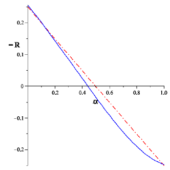
Figure 1: $-R$ for an ideal anyon gas of particles obeying fractional statistics as a function of the parameter $\alpha$ that specifies the particle content: $\alpha=0$ corresponds to bosons, $\alpha=1$ to fermions, and $0<\alpha<1$ to intermediate statistics. The dot-dashed line is for the classical limit and the continuous one shows the change in $R$ due to non-classical behavior. Figure from Mirza:2008fy , where their scalar curvature corresponds to $-R$ with our definition.

Finally, the sign of $R$ can hide information on the underlying interactions for black holes. For example, in Sahay:2010tx one shows that the scalar curvature remains negative for the metastable phase of the black hole, but changes sign at the Hawking-Page transition temperature that, therefore, can be associated with the condition $R=0$.

III Power series expansion of the scalar curvature in 2D

In this paper we investigate the thermodynamic geometry of the deconfinement transition by considering two thermodynamic variables, $\beta=1/T$ and $\gamma^{2}$, i.e. a 2-dimensional thermodynamic metric (see Eq. (9)).

In the high temperature regime the phase of strong interacting matter is described by QCD lattice simulations, reliable at low baryon density, and therefore in the calculation of the potential $\phi=P/T$ we consider a power series expansion in $\gamma^{2}<1$.

By the expression of the pressure $P$ as a power series around the point $\mu_{B}=0$,

$$P(\beta,\gamma)=P_{0}+P_{2}\,\gamma^{2}+P_{4}\,\gamma^{4}+P_{6}\,\gamma^{6}+\cdots\ ,$$ (12)

the thermodynamical potential $\phi=P/T$, the metric tensor $g_{ij}=\phi_{,ij}$ and the scalar curvature $R$ can be express by analogous power series (see App. A), i.e.

$$\phi(\beta,\gamma)=A(\beta)+B(\beta)\gamma^{2}+C(\beta)\gamma^{4}+D(\beta)\gamma^{6}+\cdots\;,$$ (13)

$$R(\beta,\gamma)=\sum_{n=0}R_{\mathcal{O}(2\,n)}(\beta)\;\gamma^{2\,n}\;.$$ (14)

The coefficients of the thermodynamical potential are given by

$$\begin{split}A(\beta)=&P_{0}(\beta)\;\beta\;,\\ B(\beta)=&P_{2}(\beta)\,\beta=\frac{\chi_{2}(\beta)}{2!\;\beta^{3}}\;,\\ C(\beta)=&P_{4}(\beta)\,\beta=\frac{\chi_{4}(\beta)}{4!\;\beta^{3}}\;,\\ D(\beta)=&P_{6}(\beta)\,\beta=\frac{\chi_{6}(\beta)}{6!\;\beta^{3}}\;,\end{split}$$ (15)

where $\chi_{2n}=\frac{\partial^{2n}}{\partial\gamma^{2n}}(P\;\beta^{4})|_{\gamma=0}=(2n)!\;P_{2n}\,\beta^{4}$.

The coefficients $R_{\mathcal{O}(2n)}$ are functions of $A$, $B$, $\ldots$ in Eqs. (13, 15) and of their derivatives with respect to $\beta$. Particularly, one can see that the $2n$-coefficient $R_{\mathcal{O}(2n)}$ is a function of the first $2(n+1)$ coefficients of the expansion for the potential $\phi$ in Eq. (13). For example, the zero-order term, $R_{\mathcal{O}(0)}$, depends on the first and second coefficients of the $\phi$ series expansion and it is given by

$$\begin{split}R_{\mathcal{O}(0)}=&\frac{1}{2}\,\frac{B^{\prime}}{A^{\prime\prime}\,B}\left(\frac{A^{\prime\prime\prime}}{A^{\prime\prime}}-\frac{B^{\prime}}{B}\right)=\\ =&\frac{1}{2\;\ddot{P}_{0}}\;\left[3+T\;\frac{\dot{\chi}_{2}}{\chi_{2}}\right]\left[\frac{\dddot{P}_{0}}{\ddot{P}_{0}}-\frac{\dot{\chi}_{2}}{\chi_{2}}\right]\;,\end{split}$$ (16)

where “$\;{}^{\prime}\;$” and “$\;\dot{\;}\;$” denote, respectively, the derivative with respect to $\beta$ and $T$; $P_{0}(\beta)$ is the pressure and $\chi_{2}(\beta)=\partial^{2}(P/T^{4})/\partial\gamma^{2}$, both at $\mu_{B}=0$. The other terms are evaluated in App. A.

In conclusion, if one knows the pressure up to $\gamma^{6}$, $g$ and $R$ can be calculated up to $\gamma^{4}$.

IV Thermodynamic Geometry of QCD

Following the results of the QCD lattice (L) simulations in ref. Bazavov:2017dus , the expansion series for the pressure is

$$P^{L}(\beta,\gamma)\simeq P^{L}_{0}+\sum_{n=1}^{\infty}\frac{P^{L}_{2n}}{\beta^{4}}\,\gamma^{2n}$$ (17)

and, by comparison with eq.(13), one gets

$$\begin{split}A^{L}=&P_{0}^{L}\;\beta\;,\\ B^{L}=&\frac{P_{2}^{L}}{\beta^{3}}\;,\\ C^{L}=&\frac{P_{4}^{L}}{\beta^{3}}\;,\\ D^{L}=&\frac{P_{6}^{L}}{\beta^{3}}\;,\end{split}$$ (18)

where, for strangeness neutral systems with a fixed ratio of electric charge to baryon density (see Bazavov:2017dus for details), one has

$$P_{2}^{L}(\beta)=\frac{1}{2}\left[N_{1}^{B}(\beta)+r\;q_{1}(\beta)\,N_{1}^{B}(\beta)\right]$$ (19)

$$\begin{split}P_{4}^{L}(\beta)=\frac{1}{4}\Big{[}&N_{3}^{B}(\beta)+r\;\Big{(}q_{1}(\beta)\,N_{3}^{B}(\beta)+\\ &\qquad+3\,q_{3}(\beta)N_{1}^{B}(\beta)\Big{)}\Big{]}\end{split}$$ (20)

$$\begin{split}P_{6}^{L}(\beta)=\frac{1}{6}\Big{[}&N_{5}^{B}(\beta)+r\;\Big{(}q_{1}(\beta)\,N_{5}^{B}(\beta)+\\ &+3\,q_{3}(\beta)N_{3}^{B}(\beta+5\;q_{5}(\beta)\,N_{1}^{B}(\beta))\Big{)}\Big{]}\;,\end{split}$$ (21)

being $N_{2n-1}^{B}$ the $(2n-1)$-th coefficient for the power expansion of the baryon number density divided by $T^{3}$,

$$\frac{n_{B}}{T^{3}}=\sum_{n=1}^{\infty}N_{2n-1}^{B}\;\gamma^{2n-1}\;,$$ (22)

$q_{2n-1}$ are the expansion coefficients for the electric charge chemical potential, and

$$r\equiv\frac{n_{Q}}{n_{B}}\;,$$ (23)

with $n_{Q}$ and $n_{B}$ the charge and baryon number densities respectively.

Three special cases are considered: the electric neutral systems, $r=0$, the isospin symmetric limit $r=1/2$, i.e. $q_{k}=0\;\forall k$, which gives the same result of $r=0$, and $r=0.4$, usually considered for applications to heavy ion collisions Bazavov:2017dus ; Bazavov:2012vg .

Figure 2 shows the scalar curvature $R$ evaluated by Eq. (14) and Eqs.(17-23). The black curves are based on lattice data with the condition $n_{S}=n_{Q}=0$ (or equivalent for the isospin symmetric limit), whereas the red ones are for $n_{S}=0$ and $n_{Q}/n_{B}=0.4$. The continuous lines are for $\mu_{B}=0$ MeV, the dashed ones for $\mu_{B}=80$ MeV and the dotted lines for $\mu_{B}=135$ MeV.

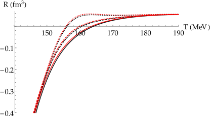
Figure 2: The scalar curvature $R$ from Eq. (14): the black curves are for lattice data obtained for the condition $n_{S}=n_{Q}=0$ (or equivalent for the isospin symmetric limit), while the reds are for $n_{S}=0$ and $n_{Q}/n_{B}=0.4$  Bazavov:2017dus ; qm18 . The continuous lines are for $\mu_{B}=0$ MeV, the dashed ones for $\mu_{B}=80$ MeV and the dotted lines for $\mu_{B}=135$ MeV.

V Thermodynamic Geometry of the Hadron Resonance Gas

The confined phase can be described in terms of a non-interacting gas of hadrons. There are several versions of the HRG which give different results ambi with some ambiguity and dependence on the specific model.

In the HRG model with point-like constituents, if $m_{max}$ is the maximum mass one includes, the trace anomaly can be written as a sum over all particles species with mass $m_{i}\leq m_{max}$ Karsch:2003vd

$$\begin{split}\left(\frac{\Theta^{\mu\mu}}{T^{4}}\right)^{H}&=\sum_{m_{i}\leq m_{max}}\frac{d_{i}}{2\,\pi^{2}}\times\\ &\times\sum_{k=1}^{\infty}\frac{(-\eta_{i})^{k+1}}{k}\left(\frac{m_{i}}{T}\right)^{3}K_{1}\left(\frac{k\,m_{i}}{T}\right)\;,\end{split}$$ (24)

where $\eta_{i}=-1(+1)$ for bosons (fermions), $K_{1}$ is the modified Bessel function, $d_{i}$ are the degeneracy factors.

For small $\mu_{B}$, the baryon sector of a HRG can be described by the Boltzmann approximation and the pressure can be written as Bazavov:2017dus

$$P^{H}(\beta,\gamma)=P^{H}_{0}(\beta)+P_{B}^{H}(\beta)\left(\cosh\gamma-1\right)\;,$$ (25)

where $P^{H}_{0}(\beta)=P_{M}^{H}(\beta)+P_{B}^{H}(\beta)$ is the total pressure at $\mu_{B}=0$ (Eq. (24)), $P_{M}^{H}(\beta)$ and $P_{B}^{H}(\beta)$ are the meson and baryon contributions to Eq. (24), respectively.

In Figure 3 are plotted the total pressure $P^{H}_{0}(\beta)$ at $\mu_{B}=0$, the meson part, $P^{H}_{M}(\beta)$, and the baryonic part, $P^{H}_{B}(\beta)$.

Figure 3: The total pressure of a HRG gas $P^{H}_{0}(\beta)$ (black line), the meson contribution $P_{M}^{H}(\beta)$ (dotted line) and the $P_{B}^{H}(\beta)$ (dot-dashed line) at $\mu_{B}=0$.

For comparison with the QCD calculations in Sec. IV, one evaluates the series expansion in $\gamma^{2}$ of Eq. (25) in the Boltzmann approximation (i.e. all baryon number susceptibilities are identical, $\chi^{H}_{2k}=\chi^{H}_{2}=2\;P_{B}^{H}\,\beta^{4}$) to obtain

$$P^{H}(\beta,\gamma)\simeq P^{H}_{0}(\beta)+\frac{\chi^{H}_{2}(\beta)}{\beta^{4}}\sum_{n=1}^{\infty}\frac{\gamma^{2n}}{(2n)!}$$ (26)

and the coefficients of the thermodynamical potential for the hadronic (H) sector are given by

$$\begin{split}A^{H}=&P_{0}^{H}\;\beta\;,\\ B^{H}=&\frac{\chi_{2}^{H}}{\beta^{3}}\;,\\ C^{H}=&\frac{2\;B^{H}}{4!}\;,\\ D^{H}=&\frac{2\;B^{H}}{6!}\;.\end{split}$$ (27)

In Fig. 4 is plotted the scalar curvature $R$ for different values of the baryonchemical potential: $\mu_{B}=0$ MeV (continuous lines), $\mu_{B}=80$ MeV (dotted lines) and $\mu_{B}=135$ MeV (dashed lines), obtained by the expansion of Eq. (14) at order $\gamma^{4}$.

Figure 4: The scalar curvature $R$, evaluated by Eqs. (26, 27) for different values of the baryonchemical potential, $\mu_{B}=0$ MeV (continuous lines), $\mu_{B}=80$ MeV (dotted lines) and $\mu_{B}=135$ MeV (dashed lines), obtained by the expansion of Eq. (14) at the 4-th order.

VI Transition temperature

In the QGP phase the system is mostly of fermionic type while in the confined phase is essentially a bosonic (mesonic) one. Moreover one knows from lattice simulation that the transition is a cross-over and therefore, following the previous discussion, the crossing temperature from QGP to a confined mesonic system can be evaluated by implementing the condition $R=0$.

In Figure 5 is plotted the critical temperature $T_{c}(\mu_{B})$ at which the scalar curvature of the QGP phase crosses the $R=0$ line, both for $r=0$ or $r=0.5$ (continuous black line) and for $n_{S}=0$ and $n_{Q}/n_{B}=0.4$ (black dotted line), compared with lattice results Bazavov:2017dus ; qm18 and the freeze-out temperature obtained by ALICE Floris:2014pta and STAR Das:2014qca ; Adamczyk:2017iwn collaborations. The yellow curve gives the crossover temperature, the blue and black grid bands are obtained by considering fixed values of the energy density (blue) or of the entropy density (grid) (see Ref. Bazavov:2017dus ; qm18 for details).

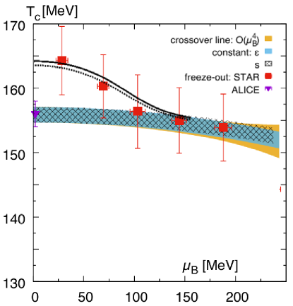
Figure 5: The crossing temperature, both for $r=0$ or $r=0.5$ (continuous black line) and for $n_{S}=0$ and $n_{Q}/n_{B}=0.4$ (black dotted line), compared with lattice data (see text qm18 ) and the results of the freeze out temperature from ALICE (purple point Floris:2014pta ) and STAR (red points Das:2014qca ; Adamczyk:2017iwn ) collaborations.

The same criterion, $R=0$ applied to the HRG gives the crossing from a mostly mesonic system to a fermion dominated one at temperature, $T_{h}$, about 20$\%$ larger than $T_{c}$.

The two different temperatures have a possible interpretation if one recalls that, since the deconfinement transition is a cross-over, one can expect remnants of confinement slightly above $T_{c}$. Indeed the persistence of string-like objects above $T_{c}$ has ben obtained by many different methods: lattice simulations karsch ; cea , quasiparticle approach mannarelli1 ; mannarelli2 , NJL correlator beppe ; jap , Mott transitions david and confinement mechanisms eddy .

Following this interpretation, $T_{c}$ is the deconfinement temperature and $T_{h}$ is the temperature of the complete melting of a light meson.

VII Comments and Conclusions

Thermodynamic geometry applied to QCD deconfinemt transition is a useful tool to evaluate the transition temperature $T_{c}$. The results, obtained by the criterion $R=0$, are in good agreement with lattice data and freeze-out calculations in the low density region. However the criterion is completely general and can be applied at large baryon density if the potential $\Phi$ can be estimated in a reliable way. On the other hand the temperature, $T_{h}$, evaluated by HRG is larger than $T_{c}$, suggesting the interpretation that the meson melting temperature is larger than the temperature associated with the chiral susceptibility. However this conclusion could be model dependent, because we have used a specific model of the HRG. The introduction of other dynamical details, as the excluded volume, could change the HRG evaluation of $R$, by including some effective repulsive interaction similar to Fermi statistic effects and then closing, in part, the gap with the value of $R$ for a fermionic system. This analysis will be carried out in a forthcoming paper.

VIII Acknowledges

The authors thank F.Karsch for the HRG data (in Fig. 3) and H.Satz for useful comments. P.Castorina thanks the Theoretical High Energy Physics Group of Bielefeld University for the hospitality.

Appendix A Power series of the scalar $R$

Let us consider the power series expansions in $\gamma^{2}$ for the pressure, i.e.

$$\begin{split}P(\beta,\gamma)=&P_{0}(\beta)+P_{2}(\beta)\,\gamma^{2}+P_{4}(\beta)\,\gamma^{4}+\\ &+P_{6}(\beta)\,\gamma^{6}+P_{8}(\beta)\,\gamma^{8}+\cdots\;,\end{split}$$ (28)

and for the potential $\Phi$,

$$\begin{split}\phi(\beta,\gamma)=&A(\beta)+B(\beta)\,\gamma^{2}+C(\beta)\,\gamma^{4}+\\ &+D(\beta)\,\gamma^{6}+E(\beta)\,\gamma^{8}+\cdots\;.\end{split}$$ (29)

The metric element $g_{11}=\phi_{11}$ and the determinant $g$ can be written respectively as

$$\begin{split}g_{11}(\beta,\gamma)=&A^{\prime\prime}+B^{\prime\prime}\,\gamma^{2}++C^{\prime\prime}\,\gamma^{4}+\\ &+D^{\prime\prime}\,\gamma^{6}+\cdots\;,\end{split}$$ (30)

$$\begin{split}g(\beta,\gamma)=&g_{\mathcal{O}(0)}+g_{\mathcal{O}(2)}\,\gamma^{2}+g_{\mathcal{O}(4)}\,\gamma^{4}+\\ &+g_{\mathcal{O}(6)}\,\gamma^{6}+\cdots\;,\end{split}$$ (31)

where

$$\begin{split}g_{\mathcal{O}(0)}(\beta)=&2B\;A^{\prime\prime}\;,\end{split}$$ (32)

$$\begin{split}g_{\mathcal{O}(2)}=&2\left(6\;C\,A^{\prime\prime}+B\,B^{\prime\prime}-2\;B^{\prime 2}\right)\;,\end{split}$$ (33)

$$\begin{split}g_{\mathcal{O}(4)}=2\Big{(}&15\,D\,A^{\prime\prime}+6\,C\,B^{\prime\prime}-\\ &\quad-8\,B^{\prime}\,C^{\prime}+B\,C^{\prime\prime}\Big{)}\;,\end{split}$$ (34)

$$\begin{split}g_{\mathcal{O}(6)}=&2\Big{(}28\,E\,A^{\prime\prime}+15\,D\,B^{\prime\prime}-12\,B^{\prime}\,D^{\prime}+\\ &\qquad+B\,D^{\prime\prime}+6\,C\,C^{\prime\prime}-8\,C^{\prime 2}\Big{)}\end{split}$$ (35)

and the symbol “^′” indicates the derivative with respect to $\beta$.

From previous equations it turns out that the $2n$-th term of the series expansion of Eq. (31) depends on the first $2(n+1)$-th terms of the expansion of $P$. Therefore, if we know the pressure up to $\gamma^{6}$, $g$ and $R$ can be evaluated at most up to $\gamma^{4}$.

To show that Eq. (28) leads to a similar series expansion for $R$, i.e.

$$\begin{split}R(\beta,\gamma)=&R_{\mathcal{O}(0)}(\beta)+R_{\mathcal{O}(2)}(\beta)\,\gamma^{2}+\\ &+R_{\mathcal{O}(4)}(\beta)\,\gamma^{4}+\cdots\;,\end{split}$$ (36)

let us define the auxiliary variable $\Gamma\equiv\gamma^{2}$ and consider the metric determinant and $R$ as a function o $\Gamma$, that is

$$\begin{split}g=&\left|\begin{array}[]{cc}\phi_{11}&2\,\sqrt{\Gamma}\;\phi_{1\widetilde{2}}\\ 2\,\sqrt{\Gamma}\;\phi_{1\widetilde{2}}&2\,\phi_{\widetilde{2}}+4\,\Gamma\;\phi_{\widetilde{2}\widetilde{2}}\end{array}\right|=\\ =&2\,\phi_{11}\,\phi_{\widetilde{2}}+4\,\Gamma\,\left[\phi_{11}\,\phi_{\widetilde{2}\widetilde{2}}-\left(\phi_{1\widetilde{2}}\right)^{2}\right]\end{split}$$ (37)

and

$$\begin{split}2\,g^{2}\,R=&4\,\phi_{1\widetilde{2}}\,\left(\phi_{\widetilde{2}}\,\phi_{111}-\phi_{11}\,\phi_{1\widetilde{2}}\right)+\\ &+8\;\Gamma\,\Big{(}\phi_{\widetilde{2}}\,\phi_{111}\,\phi_{1\widetilde{2}\widetilde{2}}-2\,\phi_{1\widetilde{2}}\,\phi_{\widetilde{2}\widetilde{2}}\,\phi_{111}+3\,\phi_{11}\,\phi_{\widetilde{2}\widetilde{2}}\,\phi_{11\widetilde{2}}+\phi^{2}_{1\widetilde{2}}\,\phi_{11\widetilde{2}}-\phi_{\widetilde{2}}\,\phi^{2}_{11\widetilde{2}}-2\,\phi_{11}\,\phi_{1\widetilde{2}}\,\phi_{1\widetilde{2}\widetilde{2}}\Big{)}+\\ &+16\;\Gamma^{2}\ \Big{(}\phi_{11}\,\phi_{11\widetilde{2}}\,\phi_{\widetilde{2}\widetilde{2}\widetilde{2}}+\phi_{1\widetilde{2}}\,\phi_{11\widetilde{2}}\,\phi_{1\widetilde{2}\widetilde{2}}+\phi_{\widetilde{2}\widetilde{2}}\,\phi_{111}\,\phi_{1\widetilde{2}\widetilde{2}}-\phi_{\widetilde{2}\widetilde{2}}\,\phi^{2}_{11\widetilde{2}}-\phi_{11}\,\phi^{2}_{1\widetilde{2}\widetilde{2}}-\phi_{1\widetilde{2}}\,\phi_{111}\,\phi_{\widetilde{2}\widetilde{2}\widetilde{2}}\Big{)}\end{split}$$

where the subscripts “$1$”,“$2$” and “$\widetilde{2}$” indicate respectively the derivative with respect to $\beta$, $\gamma$ and $\Gamma$. This expression is formally exact and the replacement of $\Phi$ as a power series of $\Gamma$ gives the final result.

Finally the terms in Eq. (36) are

$$R_{\mathcal{O}(0)}(\beta)=\frac{B^{\prime}}{2BA^{\prime\prime}}\left(\frac{A^{\prime\prime\prime}}{A^{\prime\prime}}-\frac{B^{\prime}}{B}\right)\;,$$ (38)

$$\begin{split}R_{\mathcal{O}(2)}(\beta)=&-\frac{B^{\prime}}{2\,BA^{\prime\prime}}\left(\frac{A^{\prime\prime\prime}}{A^{\prime\prime}}-\frac{B^{\prime}}{B}\right)\left(\frac{6C}{B}+\frac{B^{\prime\prime}}{A^{\prime\prime}}-\frac{2\,B^{\prime 2}}{BA^{\prime\prime}}\right)-\frac{B^{\prime\prime 2}-3A^{\prime\prime\prime}C^{\prime}}{B\,A^{\prime\prime 2}}+\frac{6\;C\,A^{\prime\prime}\,B^{\prime\prime}}{B^{2}\,A^{\prime\prime 2}}+\\ &+\frac{B^{\prime}}{2BA^{\prime\prime}}\left(\frac{B^{\prime\prime\prime}}{A^{\prime\prime}}-\frac{6\,C\,A^{\prime\prime\prime}}{B\,A^{\prime\prime}}-\frac{12\,C^{\prime}}{B}\right)+\frac{B^{\prime 2}B^{\prime\prime}}{2B^{2}A^{\prime\prime 2}}\;,\end{split}$$ (39)

$$\begin{split}R_{\mathcal{O}(4)}(\beta)=&\frac{B^{\prime}}{2\,B\,A^{\prime\prime}}\left(\frac{A^{\prime\prime\prime}}{A^{\prime\prime}}-\frac{B^{\prime}}{B}\right)\Bigg{[}3\left(\frac{6C}{B}+\frac{B^{\prime\prime}}{A^{\prime\prime}}-\frac{2\,B^{\prime 2}}{B\,A^{\prime\prime}}\right)^{2}-\frac{30\,D}{B}-\frac{12\,C\,B^{\prime\prime}}{B\,A^{\prime\prime}}+\frac{16\,B^{\prime}\,C^{\prime}}{B\,A^{\prime\prime}}-\frac{2\,C^{\prime\prime}}{A^{\prime\prime}}\Bigg{]}-\\ &-\frac{1}{B\,A^{\prime\prime}}\left(\frac{6\,C}{B}+\frac{B^{\prime\prime}}{A^{\prime\prime}}-\frac{2\,B^{\prime 2}}{B\,A^{\prime\prime}}\right)\Bigg{[}-\frac{2\,\left(B^{\prime\prime 2}-3A^{\prime\prime\prime}C^{\prime}\right)}{A^{\prime\prime}}+\frac{12\,C\,B^{\prime\prime}}{B}+\frac{B^{\prime 2}B^{\prime\prime}}{B\,A^{\prime\prime}}-\\ &\qquad\quad\qquad\quad\qquad\quad\qquad\quad\qquad\quad-B^{\prime}\left(\frac{6CA^{\prime\prime\prime}}{B\,A^{\prime\prime}}+\frac{12\,C^{\prime}}{B}-\frac{B^{\prime\prime\prime}}{A^{\prime\prime}}\right)\Bigg{]}+\\ &+\frac{1}{2\,B\,A^{\prime\prime}}\Bigg{[}\frac{15\,A^{\prime\prime\prime}D^{\prime}}{A^{\prime\prime}}+\frac{60\,D\,B^{\prime\prime}}{B}+\frac{24\,C\,C^{\prime\prime}}{B}-\frac{36\,C^{\prime 2}}{B}-\frac{45DA^{\prime\prime\prime}B^{\prime}}{BA^{\prime\prime}}-\frac{30\,D^{\prime}B^{\prime}}{B}-\\ &\qquad\quad\qquad\quad-\frac{6\,B^{\prime}C\,B^{\prime\prime\prime}}{BA^{\prime\prime}}+\frac{B^{\prime}C^{\prime\prime\prime}}{A^{\prime\prime}}-\frac{8\,B^{\prime\prime}C^{\prime\prime}}{A^{\prime\prime}}+\frac{3\,B^{\prime 2}C^{\prime\prime}}{BA^{\prime\prime}}\Bigg{]}+\\ &+\frac{C^{\prime}\left(6CA^{\prime\prime\prime}+3BB^{\prime\prime\prime}+2B^{\prime}B^{\prime\prime}\right)}{B^{2}A^{\prime\prime 2}}\end{split}$$ (40)

References

- (1) For a recent review see F.Karsch, Acta Phys.Polon.Supp. 10 (2017) 615.
- (2) For an introduction and a recent summary of results see: F. Becattini, An introduction to the Statistical Hadronization Model , arXiv:0901.3643 [hep-ph]
- (3) F.Becattini, M. Bleicher, T. Kollegger, T. Schuster, J. Steinheimer and R.Stock, Phys.Rev.Lett. 111 (2013) 082302.
- (4) P. Castorina, M. Imbrosciano and D. Lanteri, arXiv:1807.01630.
- (5) C. R. Rao, “Information and accuracy attainable in the estimation of statistical parameters”, Mathematical Society, 37 (1945) 81-91.
- (6) S. Amari, “Differential-Geometrical Methods in Statistics” L. N. Stat. 28 (1985)
- (7) F. Weinhold, J. Chem. Phys. 63 (1975) 2479, 2484, 2488, 2496.
- (8) G. Ruppeiner, “Thermodynamics: A Riemannian geometric model”, Phys. Rev. A 20 (1979) 1608.
- (9) Salamon P. and Berry R.S., “Thermodynamic length and dissipated availability”, Phys. Rev. Lett. 51, 1127 (1983)
- (10) Salamon P., Nulton J.D. and Ihrig E., “On the relation betweeen energy and entropy versions of thermodynamic lengths”, J. Chem. Phys. 80, 436 (1984).
- (11) G.E. Crooks, “Measuring Thermodynamic Length” Phys. Rev. Lett. 99, 100602 (2007)
- (12) L.D. Landau and E.M. Lifshitz, “Statistical Physics” Pergamon, New York, 1977
- (13) R.F. Greene and H.B. Callen, “On the formalism of thermodynamic fluctuation theory” Phys. Rev. 83, 1231, (1951)
- (14) G. Ruppeiner, “Riemannian geometry in thermodynamic fluctuation theory”, Rev. Mod. Phys. 67 (1995) 605-659, [Erratum: Rev. Mod. Phys. 68(1996) 313]
- (15) H. Janyszek and R. Mrugala, “Riemannian and Finslerian Geometry and Fluctuations of Thermodynamic Systems” Adv. Therm. 3 (1990)
- (16) H.-O. May, P. Mausbach, and G. Ruppeiner, “Thermodynamic curvature for attractive and repulsive intermolecular forces”, Phys. Rev. E88 (2013) 032123.
- (17) H.-O. May, P. Mausbach, and G. Ruppeiner, “Thermodynamic Geometry of Supercooled Water”, Phys. Rev. E91 (2015) 032141.
- (18) G. Ruppeiner, George ans Dyjack, A. McAloon, and J. Stoops, “Solid-like features in dense vapors near the fluid critical point”, The Journal of Chemical Physics 146 (2017) 224501.
- (19) G. Ruppeiner, A. Sahay, T. Sarkar, and G. Sengupta, “Thermodynamic Geometry, Phase Transitions, and the Widom Line”, Phys. Rev. E86 (2012) 052103.
- (20) G. Ruppeiner, “Thermodynamic curvature from the critical point to the triple point”, Phys. Rev. E86 (2012) 021130.
- (21) H.-O. May and P. Mausbach, “Riemannian geometry study of vapor-liquid phase equilibria and supercritical behavior of the lennard-jones fluid”, Phys. Rev. E85 (2012) 031201. [Erratum: Phys. Rev. E86, 059905].
- (22) A. Dey, P. Roy, and T. Sarkar, “Information geometry, phase transitions, and the Widom line: Magnetic and liquid systems”, Physica A392 (2013) 6341-6352.
- (23) P. Chaturvedi, A. Das, and G. Sengupta, “Thermodynamic Geometry and Phase Transitions of Dyonic Charged AdS Black Holes”, Eur. Phys. J. C77 no. 2 (2017) 110.
- (24) A. Sahay and R. Jha, “Geometry of criticality, supercriticality and hawking-page transitions in gauss-bonnet-ads black holes”, Phys. Rev. D96 no. 12 (2017) 126017.
- (25) H. Janyszek and R. Mrugaa, “Riemannian geometry and stability of ideal quantum gases”, J. Phys. A: Math. Gen. 23 no. 4 (1990) 467.
- (26) H. Oshimadag, T. Obataddag and H. Hara. “Riemann scalar curvature of ideal quantum gases obeying Gentile’s statistics”, J. Phys. A: Math. Gen. 32 (1999) 6373.
- (27) M. R. Ubriaco, “The role of curvature in quantum statistical mechanics”, J. Phys.: Conf. Ser. 766 (2016) 012007.
- (28) B. Mirza and H. Mohammadzadeh, “Ruppeiner Geometry of Anyon Gas”, Phys. Rev. E78 (2008) 021127.
- (29) A. Sahay, T. Sarkar, and G. Sengupta, “On the Thermodynamic Geometry and Critical Phenomena of AdS Black Holes”, JHEP 07 (2010) 082.
- (30) F. Karsch, K. Redlich, and A. Tawfik, “Hadron resonance mass spectrum and lattice QCD thermodynamics”, Eur. Phys. J. C29 (2003) 549-556.
- (31) A. Bazavov et al., “The QCD Equation of State to from Lattice QCD”, Phys. Rev. D95 (2017) 054504.
- (32) A. Bazavov, “The QCD equation of state”, Nucl. Phys. A931 (2014) 867-871.
- (33) A. Bazavov et al., “Freeze-out Conditions in Heavy Ion Collisions from QCD Thermodynamics”, Phys. Rev. Lett. 109 (2012) 192302.
- (34) V. Vovchenko and H. Stöcker, “Surprisingly large uncertainties in temperature extraction from thermal fits to hadron yield data at LHC”, J. Phys. G44 (2017) 055103, V. Vovchenko, “Equations of state for real gases on the nuclear scale”, Phys. Rev. C96 (2017) 015206.
- (35) P. Steinbrecher talk at Quark Matter 2018, Venice 2018, to appear in the proceedings of the conference.
- (36) M. Floris, “Hadron yields and the phase diagram of strongly interacting matter”, Nucl. Phys. A931 (2014) 103-112.
- (37) S. Das, “Identified particle production and freeze-out properties in heavy-ion collisions at RHIC Beam Energy Scan program”, 2014. [EPJ Web Conf.90,08007(2015)].
- (38) L. Adamczyk et al., “Bulk Properties of the Medium Produced in Relativistic Heavy-Ion Collisions from the Beam Energy Scan Program”, Phys. Rev. C96 (2017) 044904.
- (39) S.Datta,F.Karsch,P.Petreczky and I.Wetzorke, J. Phys. G 31 (2005) S351.
- (40) P.Cea,L.Cosmai, F.Cuteri and A.Papa, EPJ Web Conference 175 (2018) 12006.
- (41) P.Castorina and M.Mannarelli, Phys. Lett. B 644 (2007) 336.
- (42) P.Castorina and M.Mannarelli, Phys. Rev. C 75 (2007) 054901.
- (43) P.Castorina, G. Nardulli and D. Zappala, Phys. Rev. D 72 (2005) 076006.
- (44) Hu Li,C.M. Shakin and Qing Sun, Phys. Rev. D 67 (2003) 114012.
- (45) A.Wergieluk, D. Blaschke, Y.L. Kalinovsky and A. Friesen, Physics of Particles and Nuclei Letters 10 (2013) 660.
- (46) E. Shuryak , arXiv:1806.10487.