Towards Better Interpretability in Deep Q-Networks
Abstract
Deep reinforcement learning techniques have demonstrated superior performance in a wide variety of environments. As improvements in training algorithms continue at a brisk pace, theoretical or empirical studies on understanding what these networks seem to learn, are far behind. In this paper we propose an interpretable neural network architecture for Q-learning which provides a global explanation of the model’s behavior using key-value memories, attention and reconstructible embeddings. With a directed exploration strategy, our model can reach training rewards comparable to the state-of-the-art deep Q-learning models. However, results suggest that the features extracted by the neural network are extremely shallow and subsequent testing using out-of-sample examples shows that the agent can easily overfit to trajectories seen during training.
Introduction
The last few years have witnessed a rapid growth of research and interest in the domain of deep Reinforcement Learning (RL) due to the significant progress in solving RL problems (?). Deep RL has been applied to a wide variety of disciplines ranging from game playing, robotics, systems to natural language processing and even biological data (?; ?; ?; ?; ?; ?). However, most applications treat neural networks as a black-box and the problem of understanding and interpreting deep learning models remains a hard problem. This is even more understudied in the context of deep reinforcement learning and only recently has started to receive attention. Commonly used visualization methods for deep learning such as saliency maps and t-SNE plots of embeddings have been applied to deep RL models (?; ?; ?). However, there are a few questions over the reliability of saliency methods including, as an example, sensitivity to simple transformations of the input (?). The problem of generalization and memorization with deep RL models is also important. Recent findings suggest that deep RL agents can easily memorize large amounts of training data with drastically varying test performance and are vulnerable to adversarial attacks (?; ?; ?).
In this paper, we propose a neural network architecture for Q-learning using key-value stores, attention and constrained embeddings, that is easier to study than the traditional deep Q-network architectures. This is inspired by some of the recent work on Neural Episodic Control (NEC) (?) and distributional perspectives on RL (?). We call this model i-DQN for Interpretable DQN and study latent representations learned by the model on standard Atari environments from Open AI gym (?). Most current work around interpretability in deep learning is based on local explanations i.e. explaining network predictions for specific input examples (?). For example, saliency maps can highlight important regions of the input that influence the output of the neural network. In contrast, global explanations attempt to understand the mapping learned by a neural network regardless of the input. We achieve this by constraining the latent space to be reconstructible and inverting embeddings of representative elements in the latent space (keys). This helps us understand aspects of the input space (images) that are captured in the latent space across inputs. Our visualizations suggest that the features extracted by the convolutional layers are extremely shallow and can easily overfit to trajectories seen during training. This is in line with the results of (?) and (?). Although our main focus is to understand learned models, it is important that the models we analyze perform well on the task at hand. To this end, we show our model achieves training rewards comparable to Q-learning models like Distributional DQN (?). Our contribution in this work is threefold:
-
•
We explore a different neural network architecture with key-value stores, constrained embeddings and an explicit soft-assignment step that separates representation learning and Q-value learning (state aggregation).
-
•
We show that such a model can improve interpretability in terms of visualizations of the learned keys (cluster), attention maps and saliency maps. Our method attempts to provide a global explanation of the model’s behavior instead of explaining specific input examples (local explanations). We also develop a few examples to test the generalization behavior.
-
•
We show that the model’s uncertainty can be used to drive exploration that reaches reasonably high rewards with reduced sample complexity (training examples) on some of the Atari environments.
Related Work
Many attempts have been made to tackle the problem of interpretability with deep learning, largely in the supervised learning case. (?) carry out an in-depth survey on interpretability with Convolutional Neural Networks (CNNs). Our approach to visualizing embeddings is in principle similar to the work of (?) on inverting visual representations. They train a neural network with deconvolution layers using HOG, SIFT and AlexNet embeddings as input and their corresponding real images as ground truth (the sole purpose of this network being visualization). Saliency maps are another popular type of method that generate local explanations which generally use gradient-like information to identify salient parts of the image. The different ways of computing saliency maps are covered exhaustively in (?). Few of these have been applied in the context of deep reinforcement learning. (?) use the Jacobian of the network to compute saliency maps on a Q-value network. Perturbation based saliency maps using a continuous mask across the image and also using object segmentation based masks have been studied in the context of deep-RL (?; ?; ?). In contrast to these approaches, our method is based on a global view of the network. Given a particular action and expected returns, we invert the corresponding key to try and understand visual aspects being captured by the embedding regardless of the input state. More recently, (?) introduce a new method that finds interpretable programs that can best explain the policy learned by a neural network- these programs can also be treated as global explanations for the policy networks.
Architecturally, our network is similar to the network first proposed by (?). The authors describe their motivation as speeding up the learning process using a semi-tabular representation with Q-value calculations similar to the tabular Q-learning case. This is to avoid the inherent slowness of gradient descent and reward propagation. Their model learns to attend over a subset of states that are similar to the current state by tracking all the states recently seen (up-to half-million states) using a k-d tree. However, their method does not have any notion of clustering or fixed Q-values. Our proposed method is also similar to ?’s work on categorical/distributional DQN. The difference is that in our model the cluster embeddings (keys) for different Q-values are accessible freely (for analysis and visualization) because of the explicit soft-assignment step, whereas it is almost impossible to find such representations while having fully-connected layers like in (?). Although we do not employ any iterative procedure (like refining keys; we train fully using backpropagation), works on combining deep embeddings with unsupervised clustering methods (?; ?) (joint optimization/iterative refinement) have started to pick up pace and show better performance compared to traditional clustering methods.
Another important direction that is relevant to our work is that of generalizing behavior of neural networks in the reinforcement learning setting. (?) discuss in detail about general problems of deep RL research and evaluation metrics used for reporting. (?; ?) perform systematic experimental studies on various factors affecting generalization behavior such as diversity in training seeds and randomness in environment rewards. They conclude that deep RL models can easily overfit to random reward structures or when there is insufficient training diversity and careful evaluation techniques (such as isolated training and testing seeds) are needed.
Proposed Method
We follow the usual RL setting and assume the environment can be modelled as a Markov Decision Process (MDP) represented by the 5-tuple , where is the state space, is the action space, is the state transition probability function, is the reward function and is the discount factor. A policy maps every state to a distribution over actions. The value function is the expected discounted sum of rewards by following policy from state at time , . Similarly, the Q-value (action-value) is the expected return starting from state , taking action and then following . Q-value function can be recursively estimated using the Bellman equation and is the optimal policy which achieves the highest over all policies .
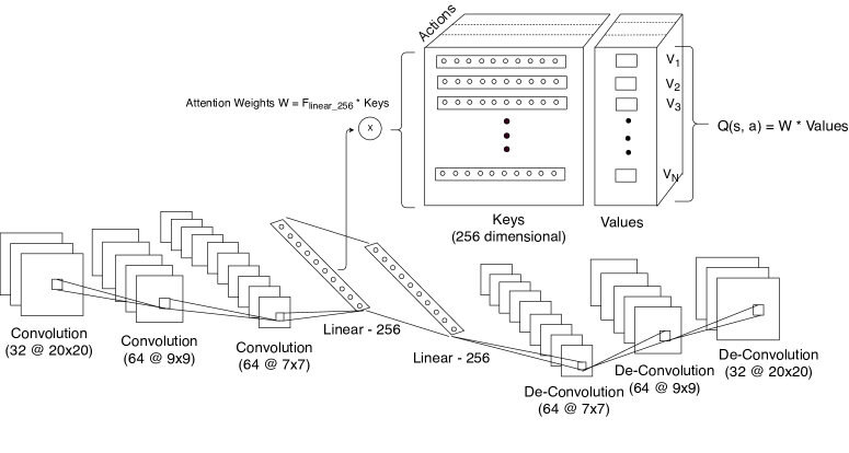
Similar to the traditional DQN architecture (?), any state (a concatenated set of input frames) is encoded using a series of convolutional layers each followed by a non-linearity and finally a fully-connected layer at the end . This would usually be followed by some non-linearity and a fully-connected layer that outputs Q-values. Instead, we introduce a restricted key-value store over which the network learns to attend as shown in Figure 1.
Intuitively, the model is trying to learn two things. First, it learns a latent representation that captures important visual aspects of the input images. At the same time, the model also attempts to learn an association between embeddings of states and embeddings of keys in the key-value store. This would help in clustering the state (around the keys) based on the scale of expected returns (Q-values) from that state. We can think of the different keys (for a given action ) weakly as the cluster centers for the corresponding Q-values, attention weights as a soft assignment between embeddings for current state and embeddings for different Q-values . This explicit association step helps us in understanding the model in terms of attention maps and visualizations of the cluster centers (keys).
The key-value store is restricted in terms of size and values of the store. Each action has a fixed number of key-value pairs (say ) and the value associated with every key is also held constant. values are sampled uniformly at random from (usually ) once and the same set of values are used for all the actions. All of the keys () are also initialized randomly. To compute attention, the embeddings for a state are compared to all the keys in the store for a particular action using a softmax over their dot products.
| (1) |
These attention weights over keys and their corresponding value terms are then used to calculate the Q-values.
Now that we have Q-values, we can define the different losses that can be used to train the network,
-
•
Bellman Error (): The usual value function estimation error.
where
-
•
Distributive Bellman Error (): We force the distributive constraint on attention weights between current and next states similar to (?) using values as supports of the distribution. The distributive loss is defined as the KL divergence between and where is the distributional Bellman operator and is the projection operator and is best action at state i.e. .
(2) (3) Equation (3) is simply the cross entropy loss (assuming to be constant with respect to , similar to the assumption for in Bellman error).
-
•
Reconstruction Error (): We also constrain the embeddings for any state to be reconstructible. This is done by transforming using a fully-connected layer and then followed by a series of non-linearity and deconvolution layers.
(4) The mean squarred error between reconstructed image and original image is used,
-
•
Diversity Error (): The diversity error forces attention over different keys in a batch. This is important because training can collapse early with the network learning to focus on very few specific keys (because both the keys and attention weights are being learned together). We could use KL-divergence between the attention weights but (?) develop an elegant solution to this in their work.
where is a 2D matrix of size (batch size, ) and each row of is the attention weight vector . It drives to be diagonal (no overlap between keys attended to within a batch) and -2 norm of to be . Because of softmax, the -1 norm is also and so ideally the attention must peak at exactly one key however in practice it spreads over as few keys as possible. Finally, the model is trained to minimize a weighted linear combination of all the four losses.
| Environment | 10M frames | Reported Scores (final) | |||||
| DDQN | i-DQN | DDQN | Distrib. DQN | Q-ensemble | Bootstrap DQN | Noisy DQN | |
| Alien | 1,533.45 | 2,380.72 | 3,747.7 | 4,055.8 | 2,817.6 | 2,436.6 | 2,394.90 |
| Freeway | 22.5 | 28.79 | 33.3 | 33.6 | 33.96 | 33.9 | 32 |
| Frostbite | 754.48 | 3,968.45 | 1,683.3 | 3,938.2 | 1,903.0 | 2,181.4 | 583.6 |
| Gravitar | 279.89 | 517.33 | 412 | 681 | 318 | 286.1 | 443.5 |
| MsPacman | 2,251.43 | 6,132.21 | 2,711.4 | 3,769.2 | 3,425.4 | 2,983.3 | 2,501.60 |
| Qbert | 10,226.93 | 19,137.6 | 15,088.5 | 16,956.0 | 14,198.25 | 15,092.7 | 15,276.30 |
| Space Invaders | 563.2 | 979.45 | 2,525.5 | 6,869.1 | 2,626.55 | 2,893 | 2,145.5 |
| Venture | 70.87 | 985.11 | 98 | 1,107.0 | 67 | 212.5 | 0 |
Experiments and Discussions
We report the performance of our model on eight Atari environments (?)- Alien, Freeway, Frostbite, Gravitar, MsPacman, Qbert, SpaceInvaders, and Venture, in Table 1. Using the taxonomoy of Atari games from (?) and (?), seven of the eight environments tested (all except SpaceInvaders) are considered hard exploration problems. Additionally, three of them (Freeway, Gravitar and Venture) are hard to explore because of sparse rewards. Since our focus is on interpretability, we do not carry out an exhaustive performance comparison. We simply show that training rewards achieved by i-DQN model are comparable to some of the state-of-the-art models. This is important because we would like our deep-learning models to be interpretable but also remain competitive at the same time. We look at scores against other exploration baselines for Q-learning that do not involve explicit reward shaping/exploration bonuses- Bootstrap DQN (?), Noisy DQN (?) and Q-ensembles (?).
Directed exploration
We use the uncertainty in attention weights to drive exploration during training. is an approximate upper confidence on the Q-values. Similar to (?) we select the action maximizing a UCB style confidence interval,
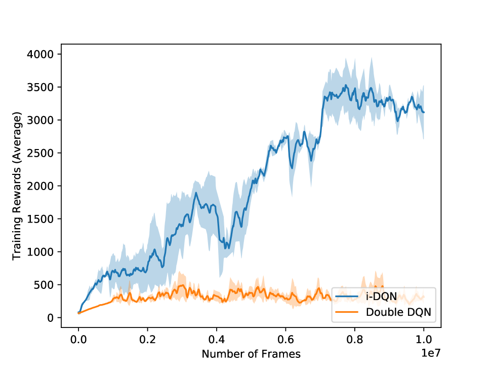
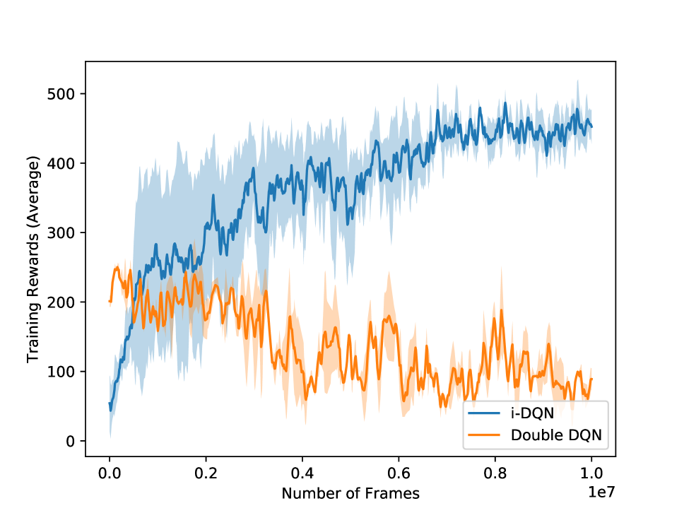
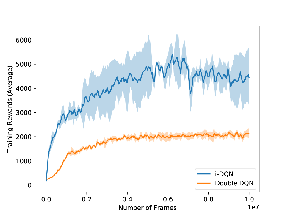
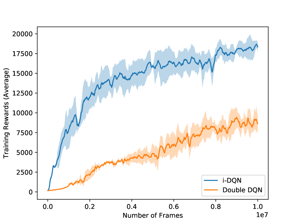
Table 1 compares i-DQN’s performance (with directed exploration) against a baseline Double DQN implementation (which uses epsilon-greedy exploration) at 10M frames. Double DQN (DDQN), Distributional DQN (Distrib. DQN), Bootstrap DQN and Noisy DQN agents are trained for up to 50M steps which translates to 200M frames (?; ?; ?). The Q-ensemble agent using UCB-style exploration is trained for up to 40M frames (?). We see that on some of the games, our model reaches higher training rewards within 10M frames compared to Double DQN, Distributional DQN models. Also, our model is competitive with the final scores reported by other exploration baselines like Bootstrap DQN, Noisy DQN and Q-ensembles, and and even performs better on some environments (5 out of 8 games). The training time for i-DQN is roughly 2x slower because of the multiple loss functions compared to our implementation of Double DQN.
What do the keys represent?
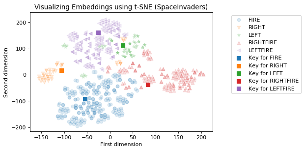
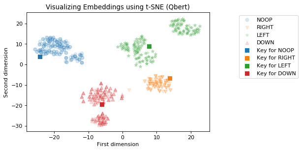
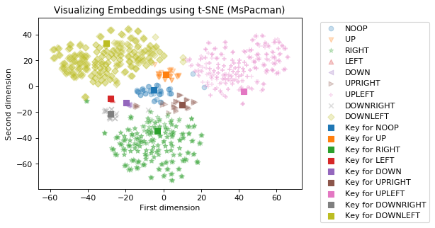
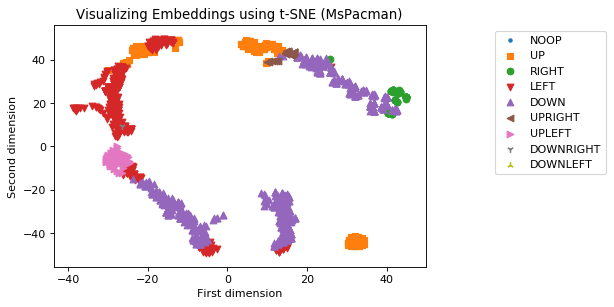
The keys are latent embeddings (randomly initialized) that behave like cluster centers for the particular action-return pairs (latent space being ). Instead of training using unsupervised methods like K-means or mixture models, we use the neural network itself to find these points using gradient descent. For example, the key for action right; Q-value 25 (Figure 2(c)) is a cluster center that represents the latent embeddings for all states where the agent expects a return of 25 by selecting action right. These keys partition the latent space into well formed clusters as shown in Figure 2, suggesting that embeddings also contain action-specific information crucial for an RL agent. On the other hand, Figure 2(d) shows embeddings for DDQN which are not easily separable (similar to the visualizations in (?)). Since we use simple dot-product based distance for attention, keys and state embeddings must lie in a similar space and this can be seen in the t-SNE visualization i.e. keys (square boxes) lie within the state embeddings (Figure 2). The fact that the keys lie close to their state embeddings is essential to interpretability because state embeddings satisfy reconstructability constraints.

Inversion of keys
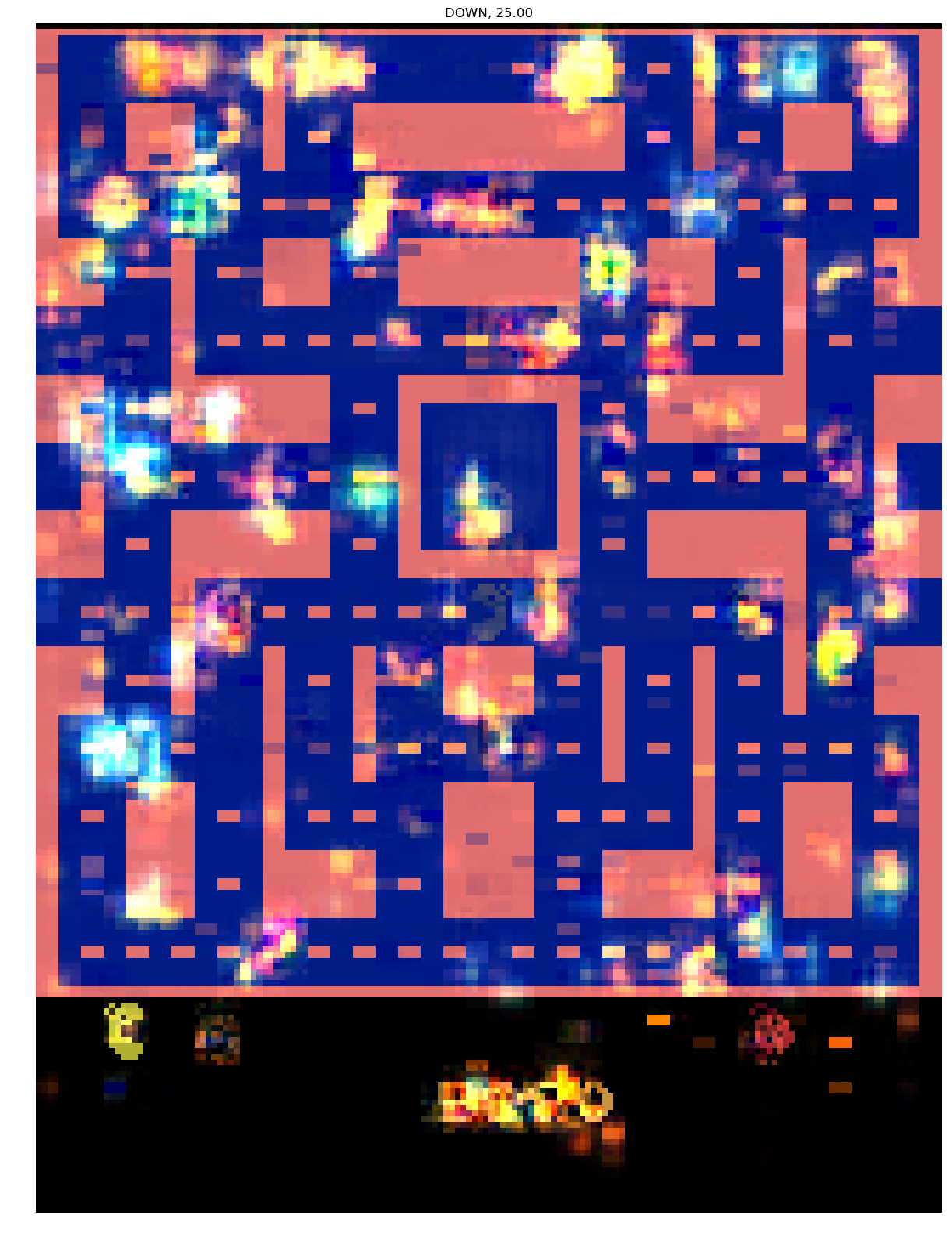
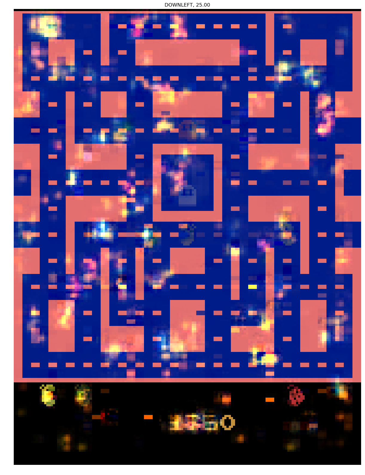
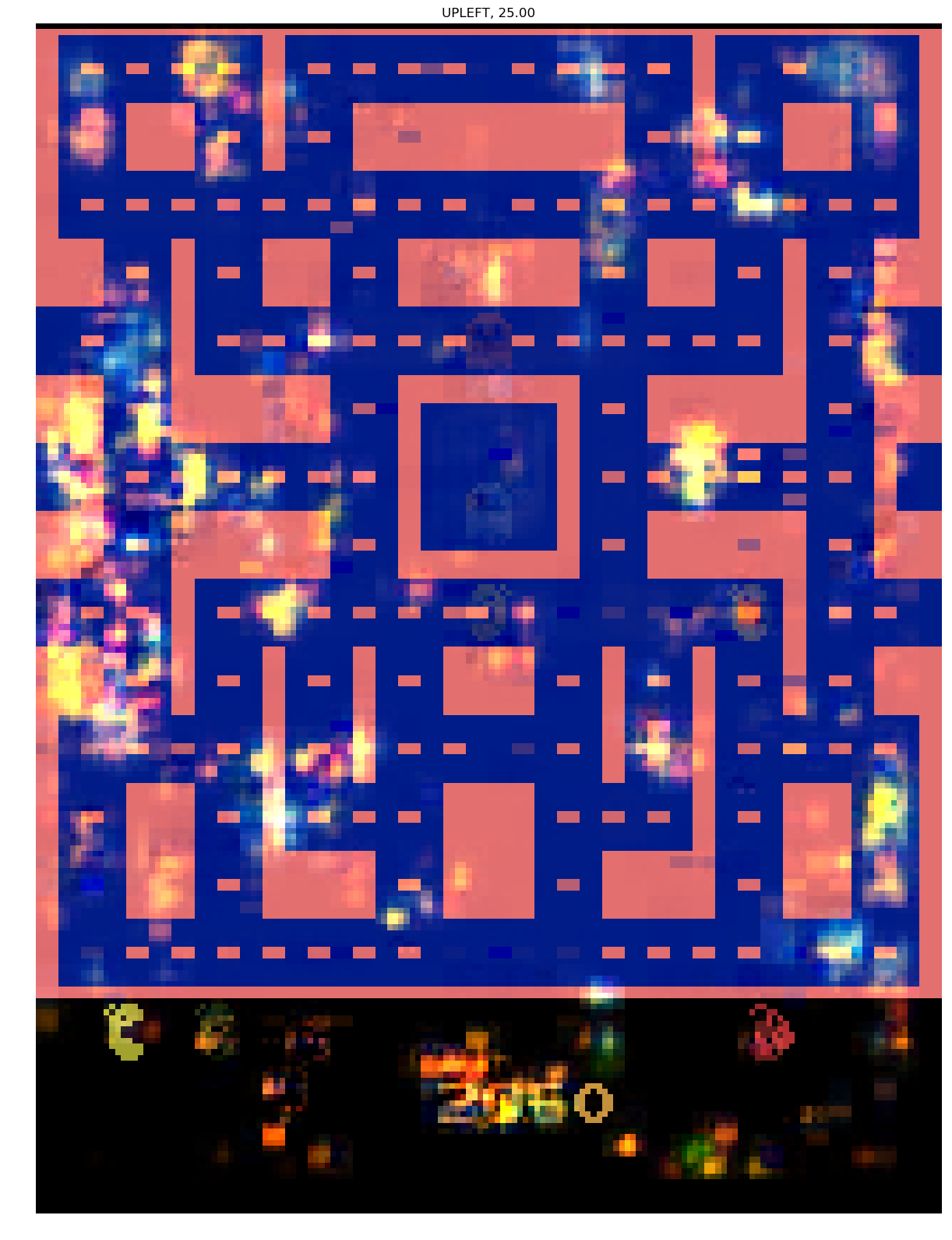
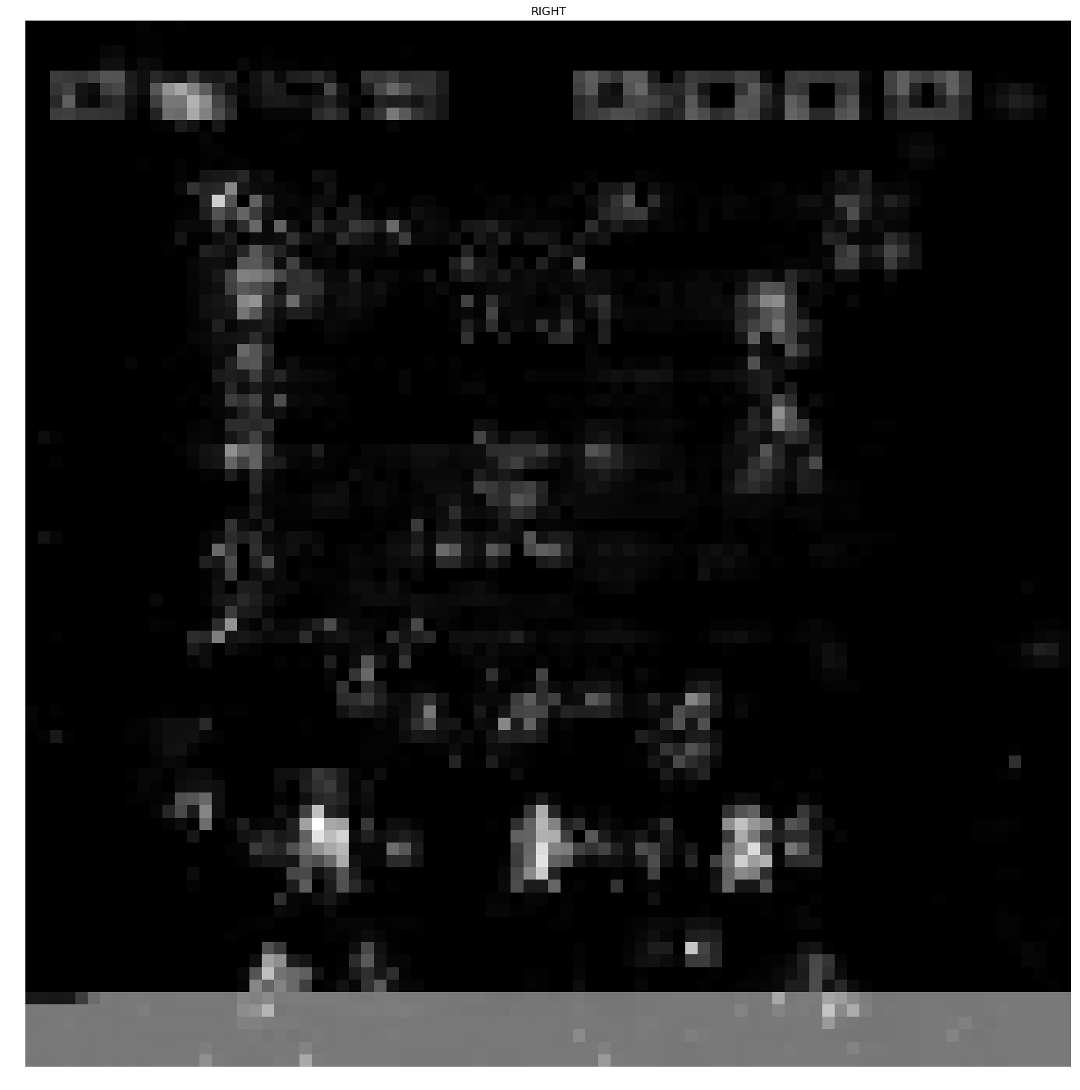
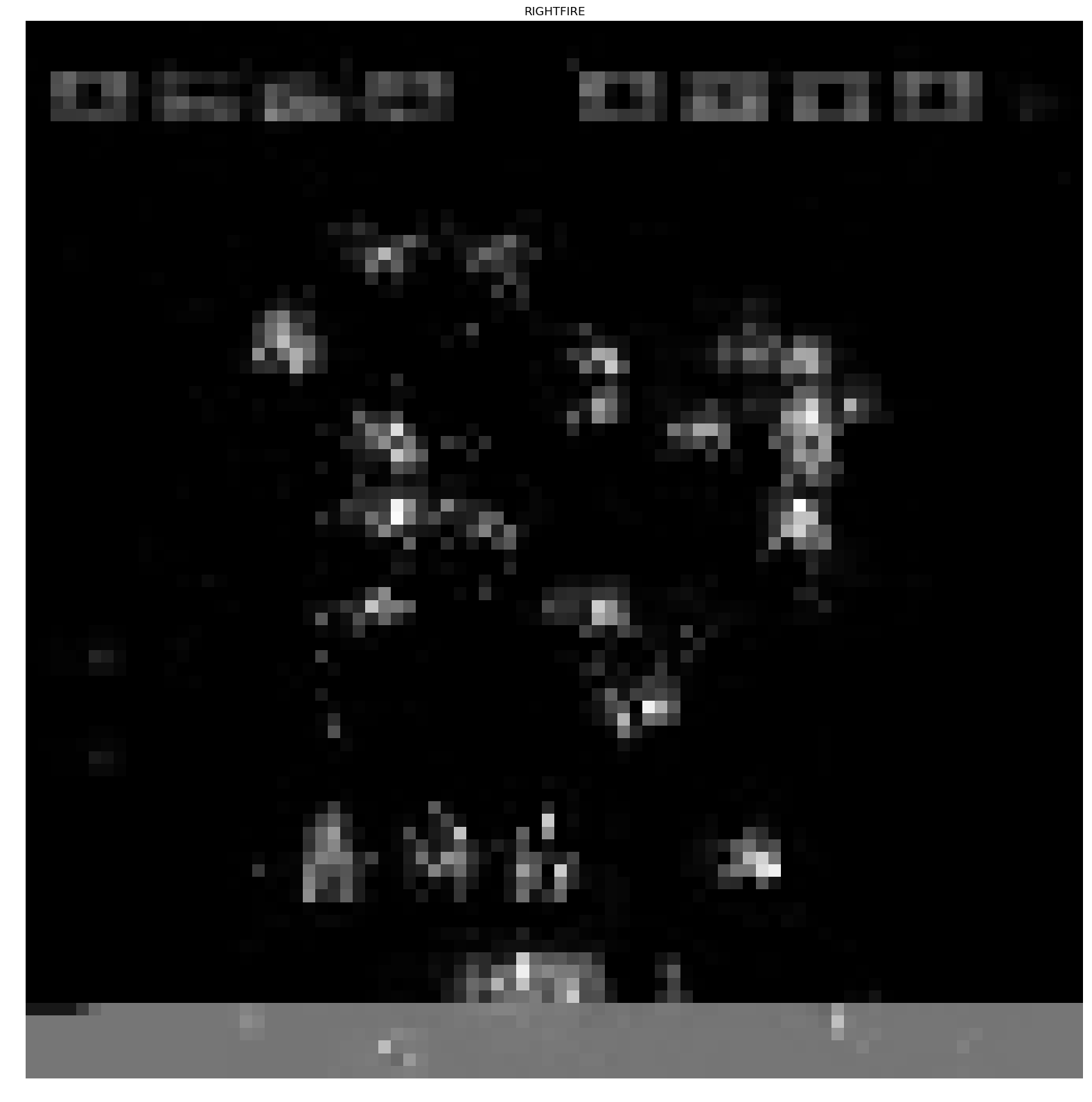
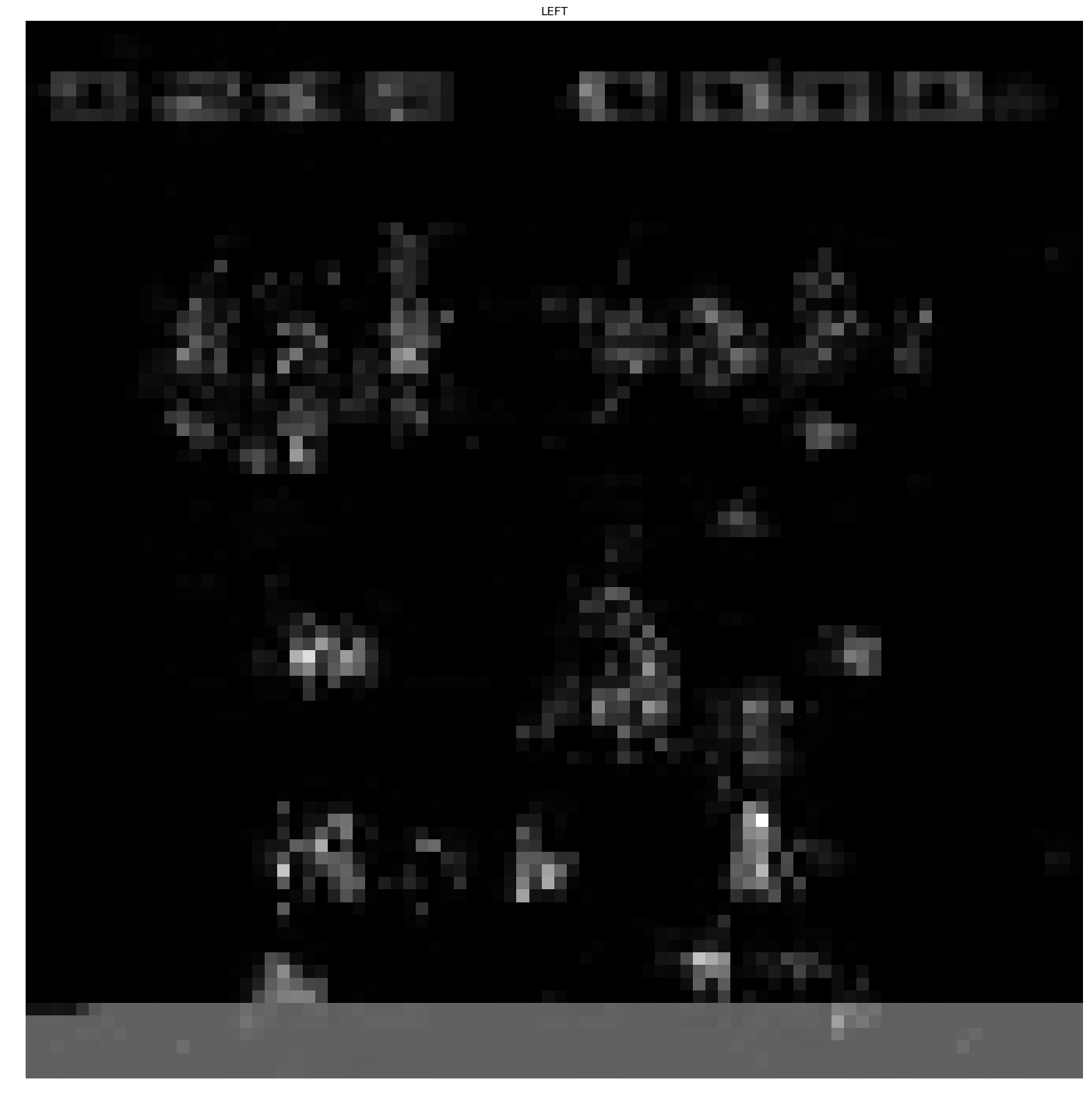
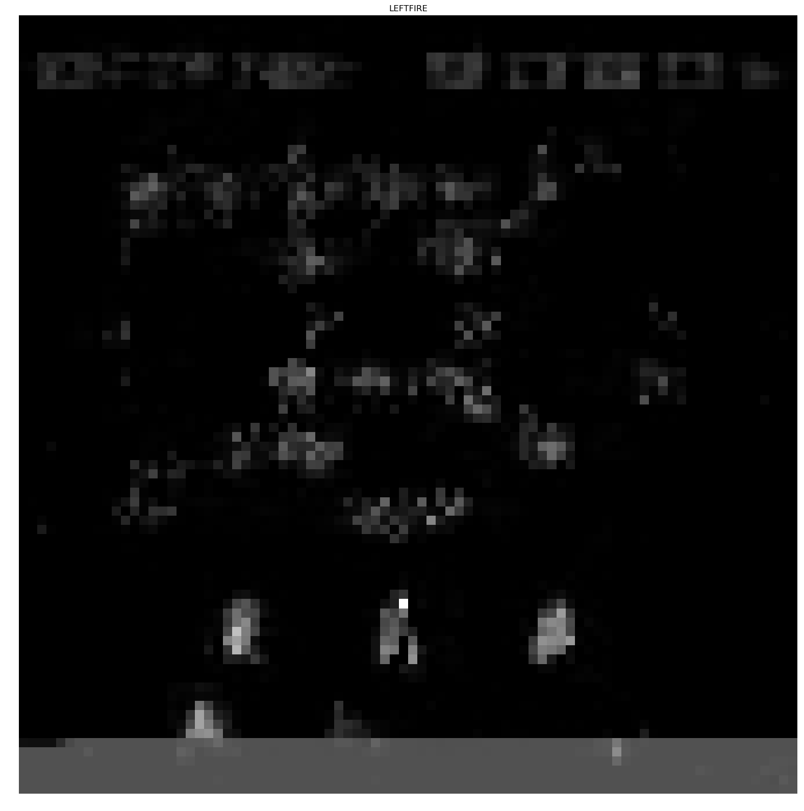
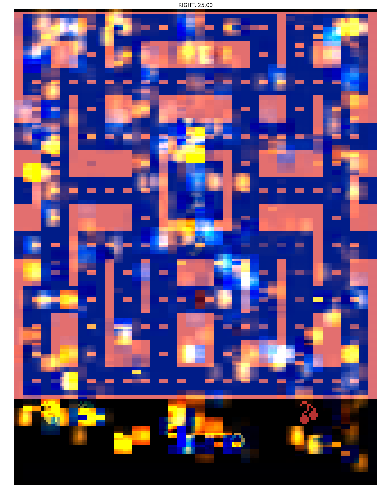
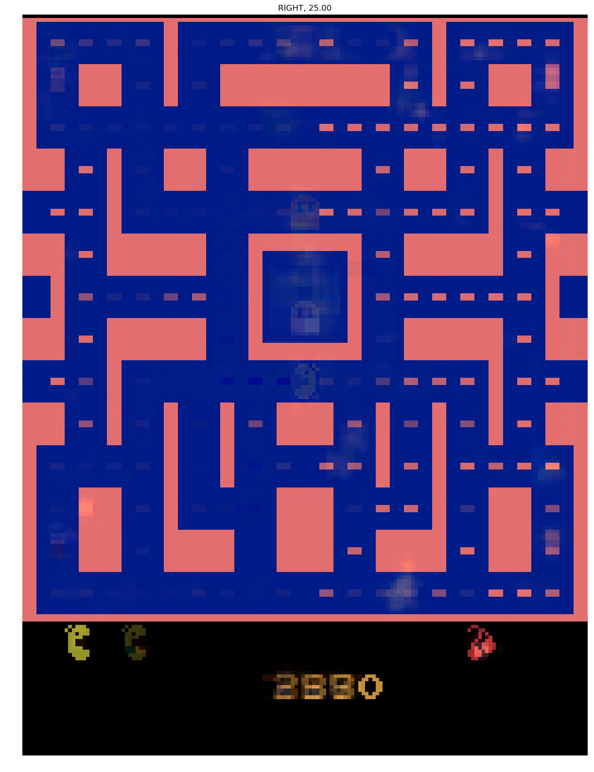
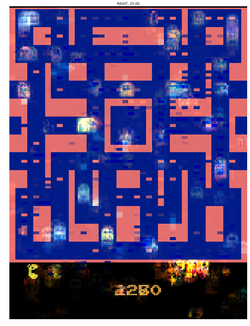
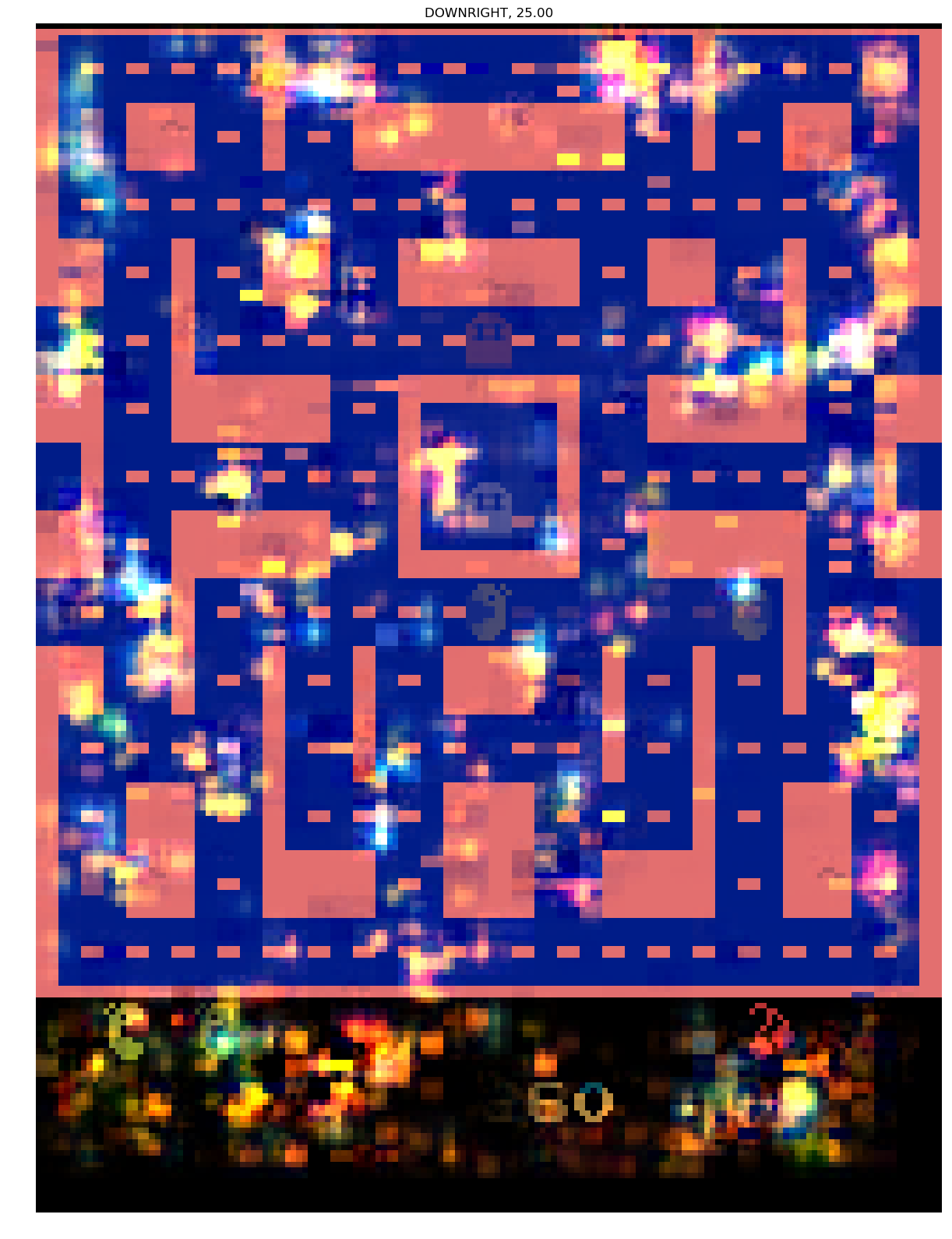
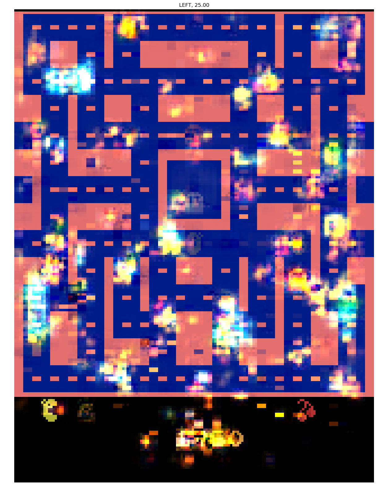
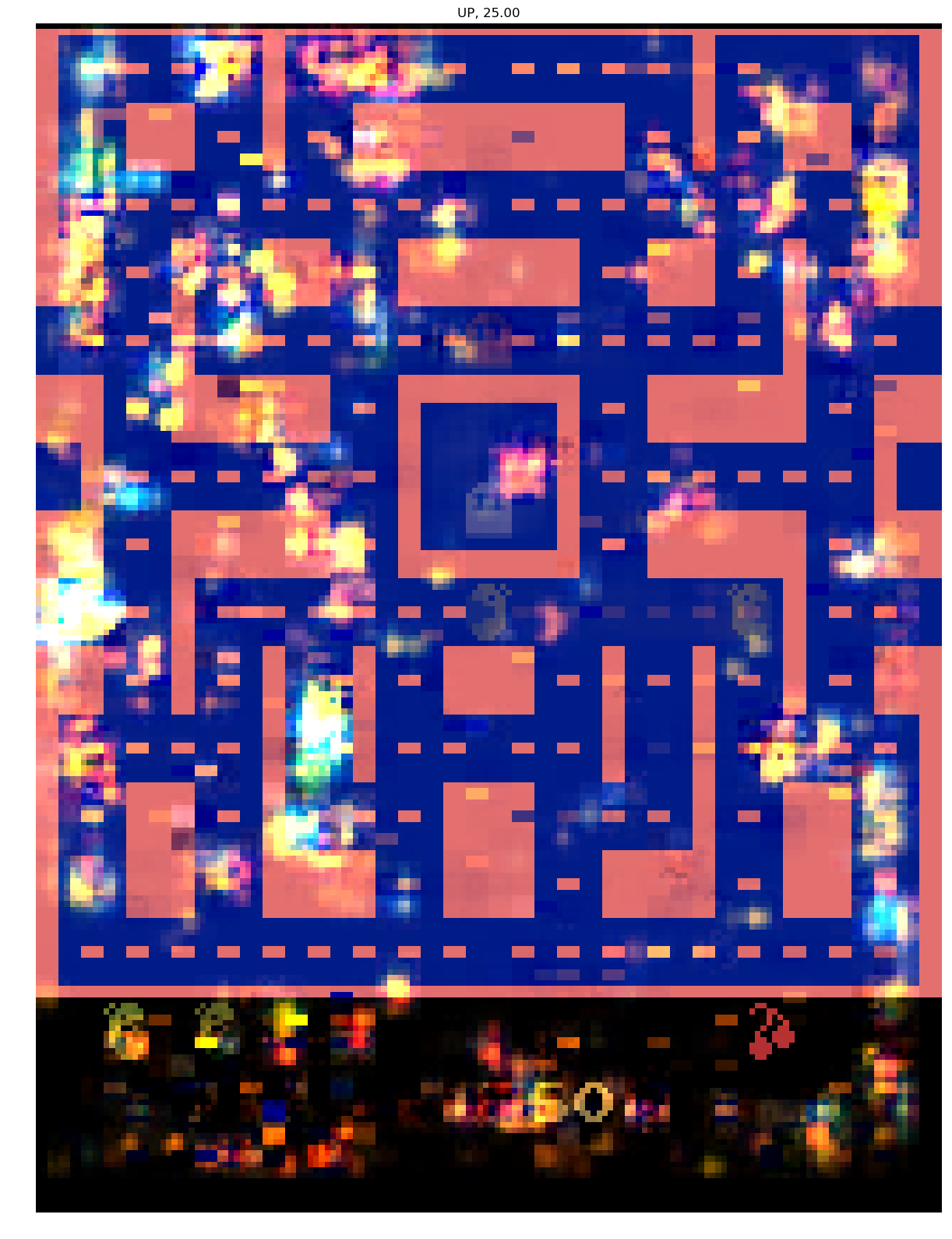
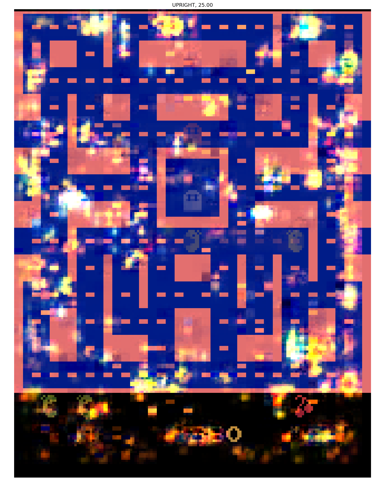
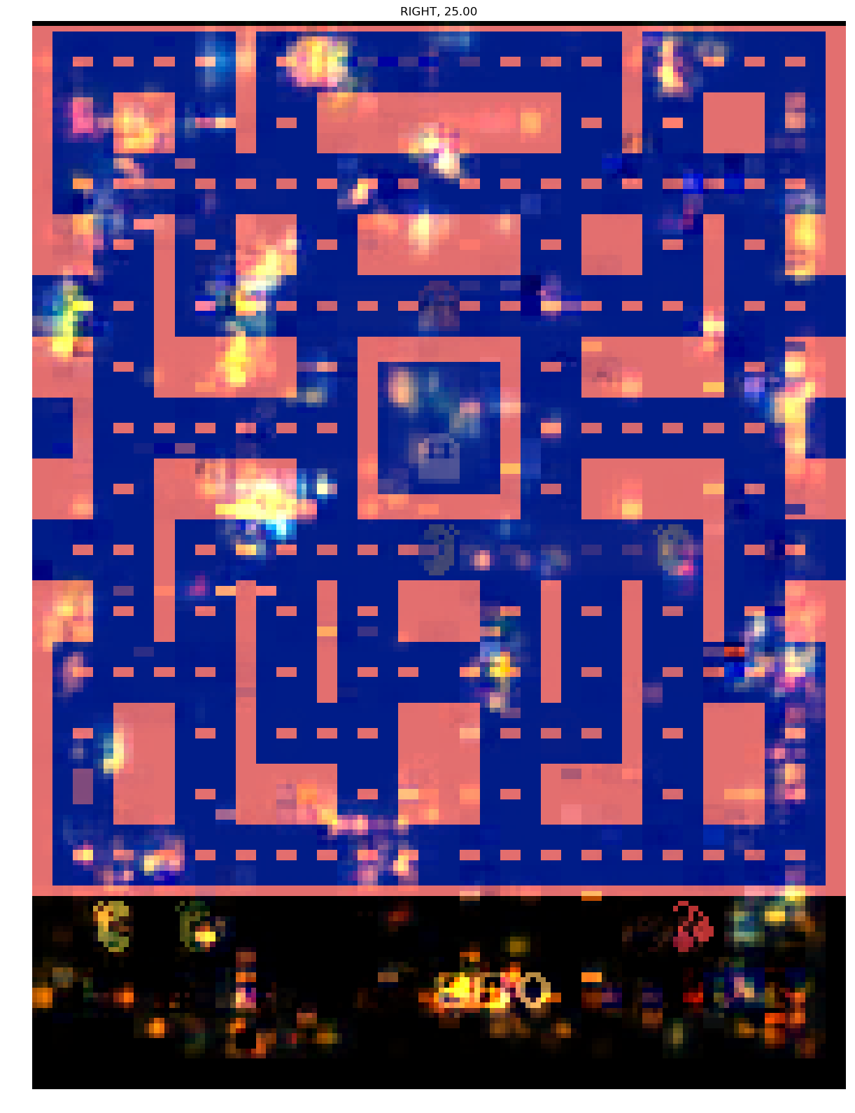
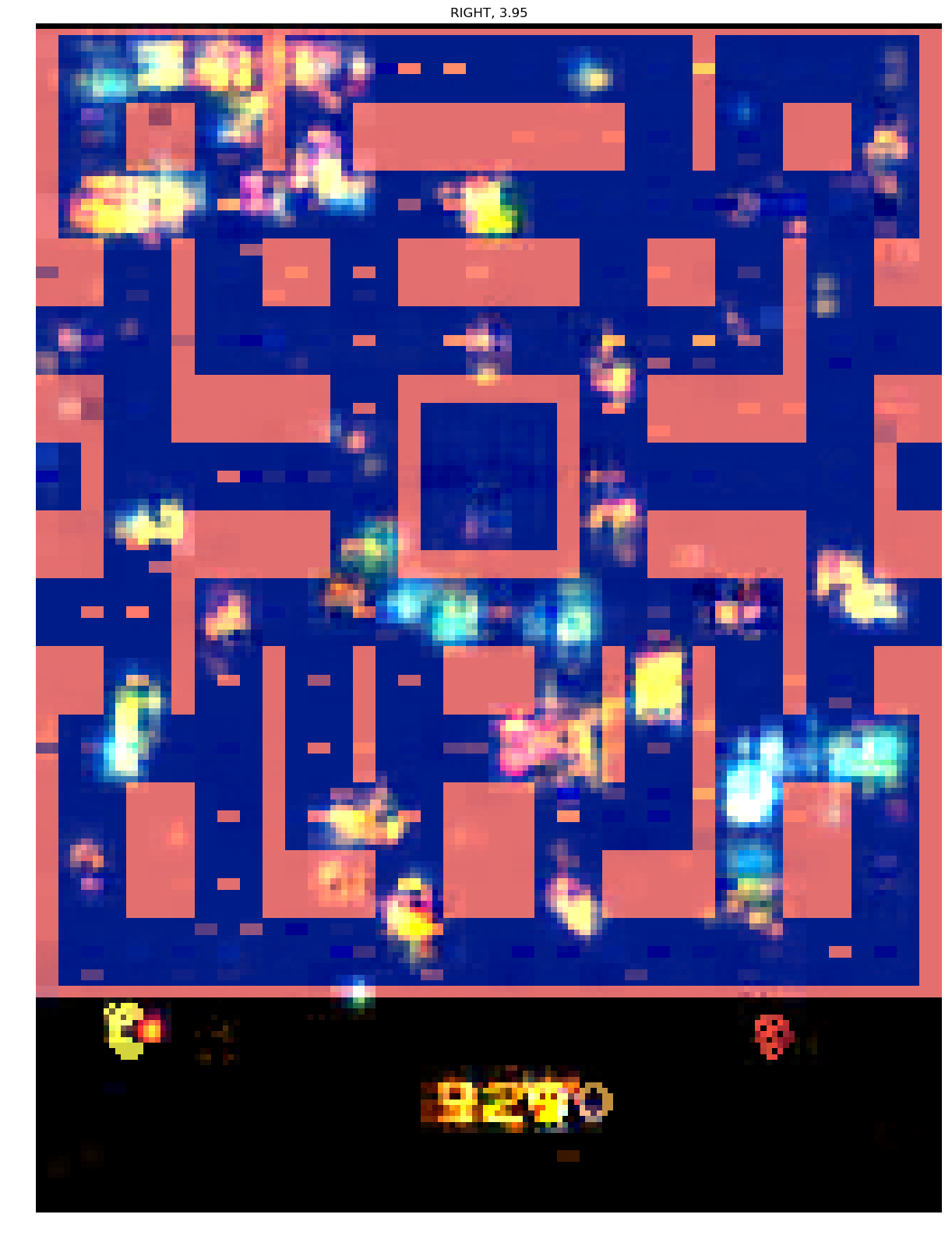
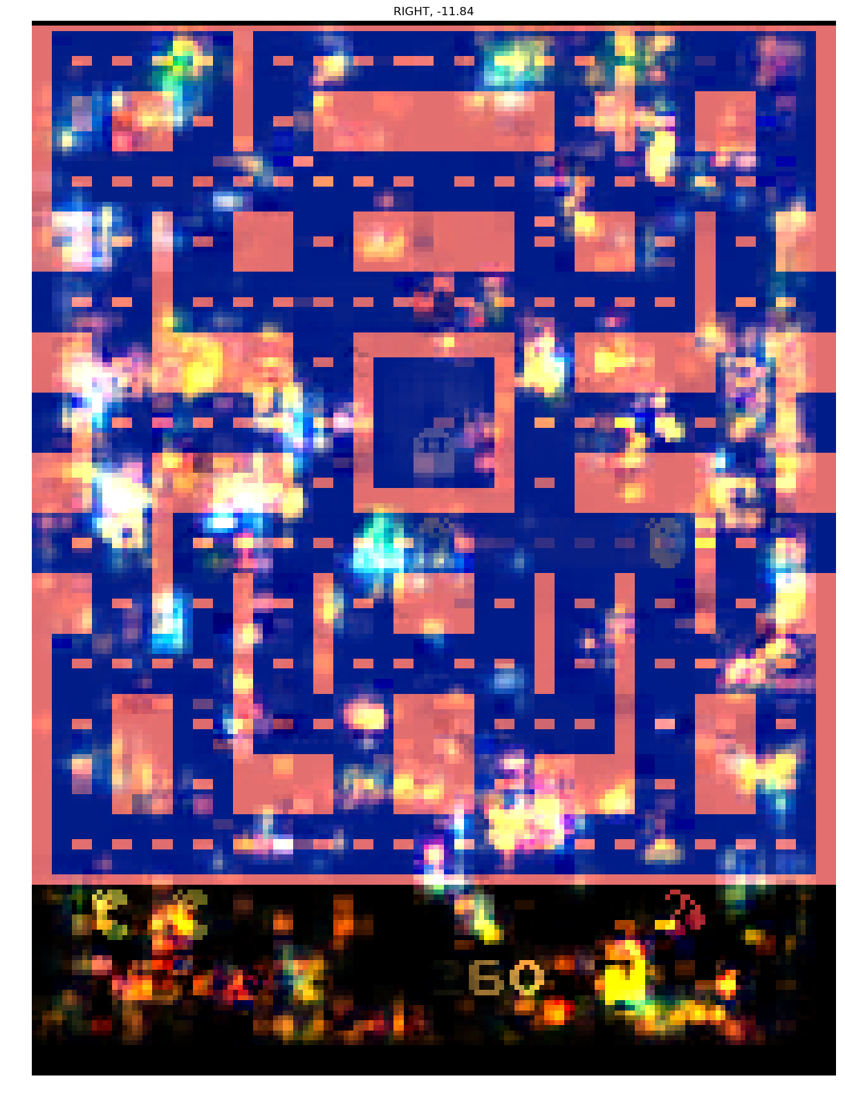
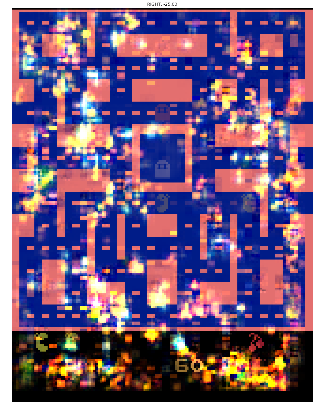
Although keys act like cluster centers for action-return pairs, it is difficult to interpret them in the latent space. By inverting keys, we attempt to find important aspects of input space (images) that influence the agent to choose particular action-return pair (). These are ‘global explanations’ because inverting keys is independent of the input. For example, in MsPacman, reconstructing keys for different actions (fixing return of 25) indicates yellow blobs at many different places for each action (Figure 4). We hypothesize that these correspond to the Pacman object itself and that the model memorizes its different positions to make its decision i.e. the yellow blobs in Figure 3(d) correspond to different locations of Pacman and for any input state where Pacman is in one of those positions, the agent selects action right expecting a return of 25. Figure 5 shows such examples where the agent’s action-return selection agrees with reconstructed key (red boxes indicate Pacman’s location). Similarly, in SpaceInvaders, the agent seems to be looking at specific combinations of shooter and alien ship positions that were observed during training (Figure 4).
The keys have never been observed by the deconvolution network during training and so the reconstructions depend upon its generalizability. Interestingly, reconstructions for action-return pairs that are seen more often tend to be less noisy with less artifacts. This can be observed in Figure 4 for Q-value 25 where actions Right, Downleft and Upleft nearly 65% of all actions taken by the agent. We also look at the effect of different reconstruction techniques keeping the action-return pair fixed (Figure 6). Variational autoencoder with set to 0 yields sharper looking images but increasing which is supposed to bring out disentanglement in the embeddings yields reconstructions with almost no objects. Dense VAE with is a slightly deeper network similar to (?) and seems to reconstruct slightly clearer shapes of ghosts and pacman.
| Agreement | AE |
|
|
|
||||||
|---|---|---|---|---|---|---|---|---|---|---|
|
30.76 | 29.78 | 16.8 | 23.73 | ||||||
|
19.87 | 18.14 | 10.97 | 14.56 |

Evaluating the reconstructions
To understand the effectiveness of these visualizations, we design a quantitative metric that measures the agreement between actions taken by the agent and the actions suggested using the reconstructed images. With a fully trained model, we reconstruct images from the keys for all actions . In every state , we induce another distribution on the Q-values using the cosine similarity in the image space,
similar to (which is also a distribution over Q-values but in the latent space). Using , we can compute and as before and select an action . Using and , we define our metric of agreeability as
where is the indicator function. We measure this across multiple rollouts (5) using and average them . In Table 2, we report Agreement as a percentage for different encoder-decoder models. Unfortunately, the best agreement between the actions selected using the distributions in the image space and latent space is around for the unscaled color version of MsPacman. In MsPacman, the agent has 9 different actions and a random strategy would expect to have an Agreement of . However, if the agreement scores were high (80-90%), that would suggest that the Q-network is indeed learning to memorize configurations of objects seen during training. One explanation for the gap is that reconstructions rely heavily on generalizability to unseen keys.
Adversarial examples that show memorization
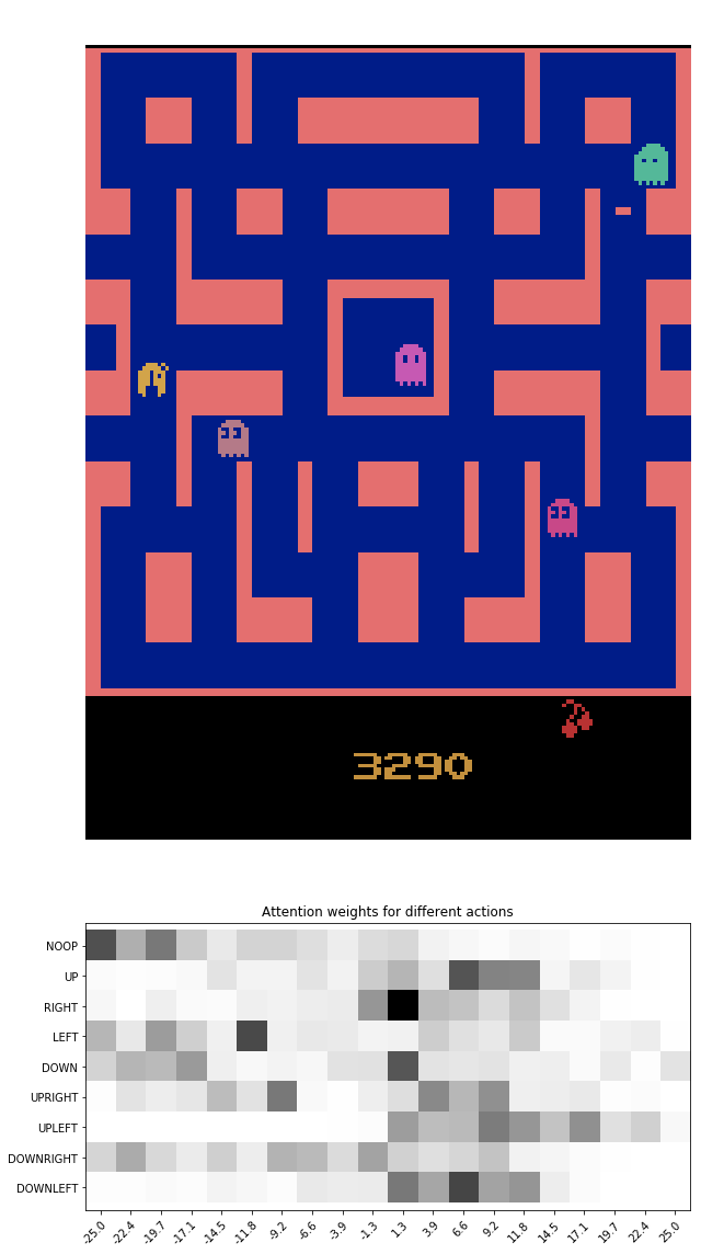
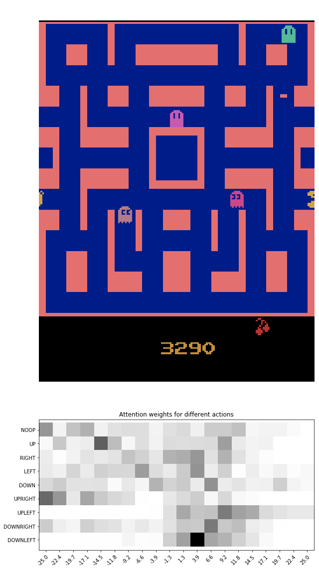
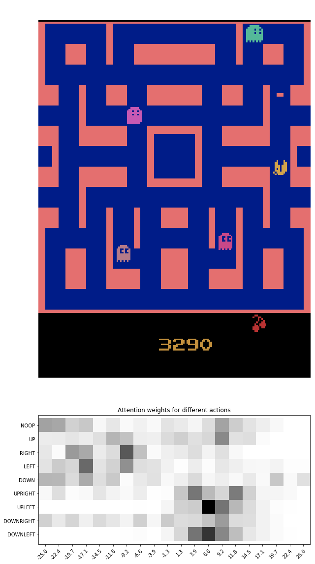
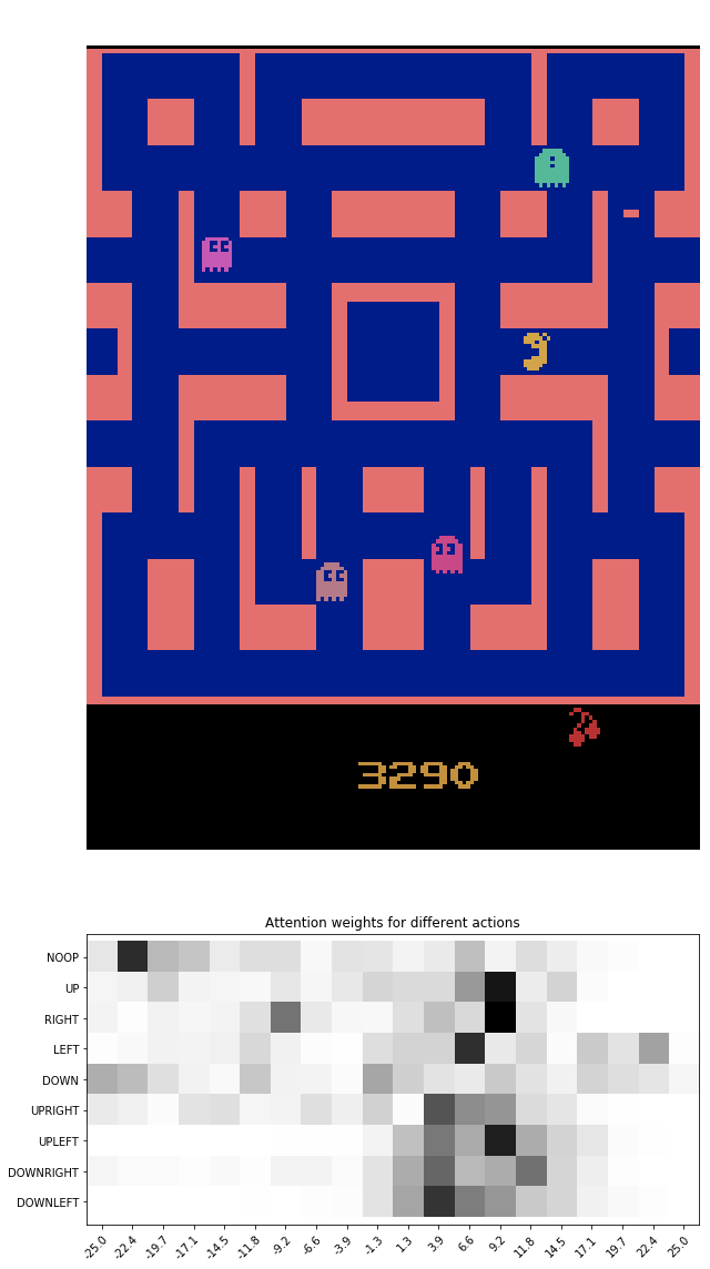
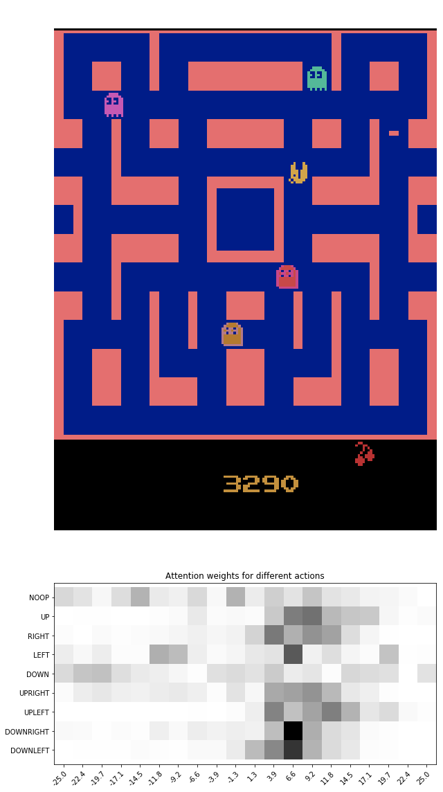
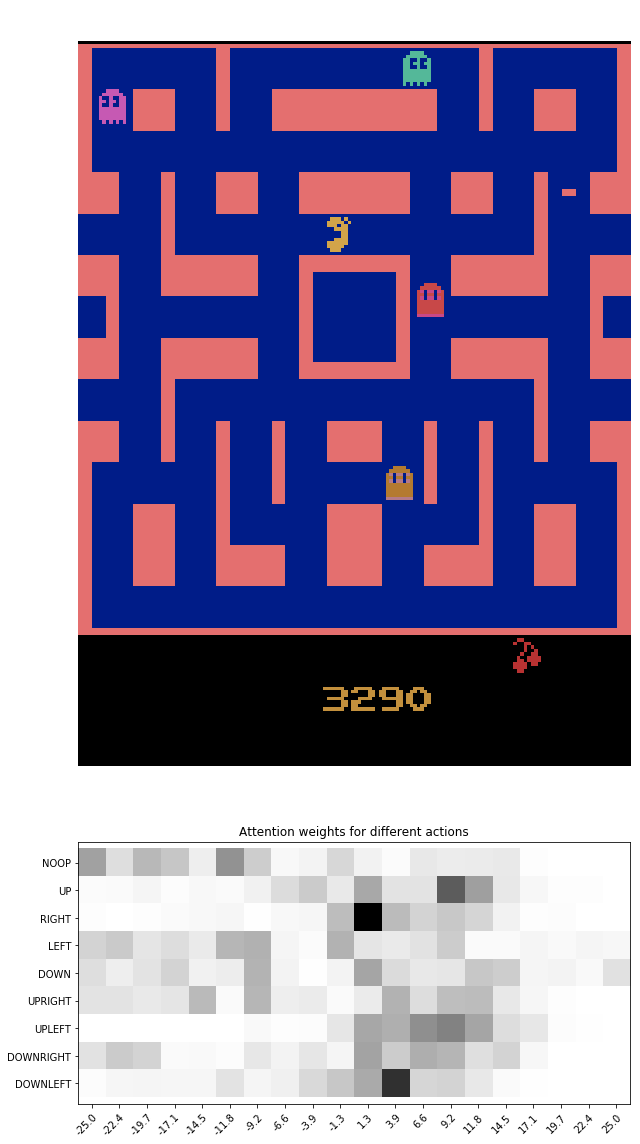
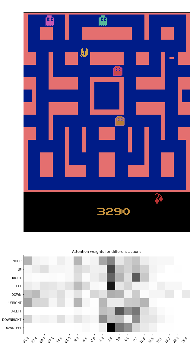
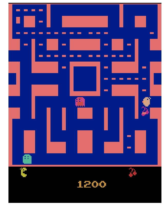
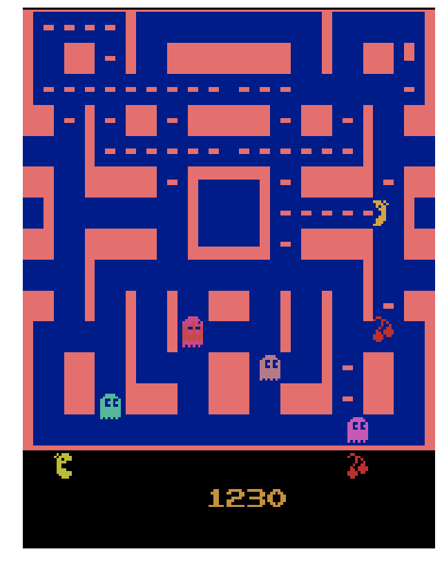
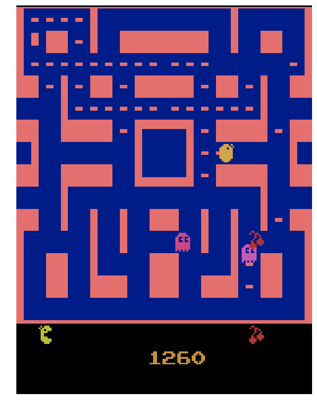
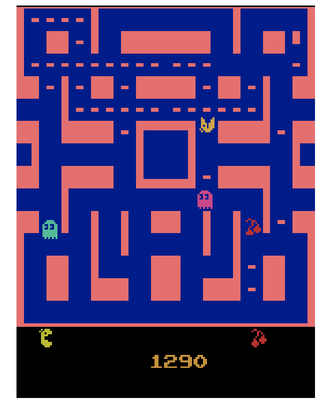
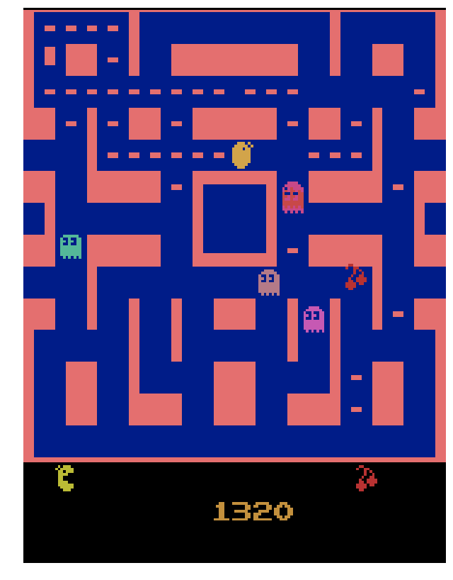
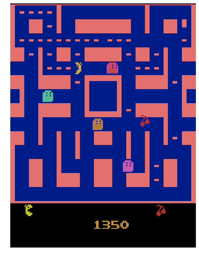
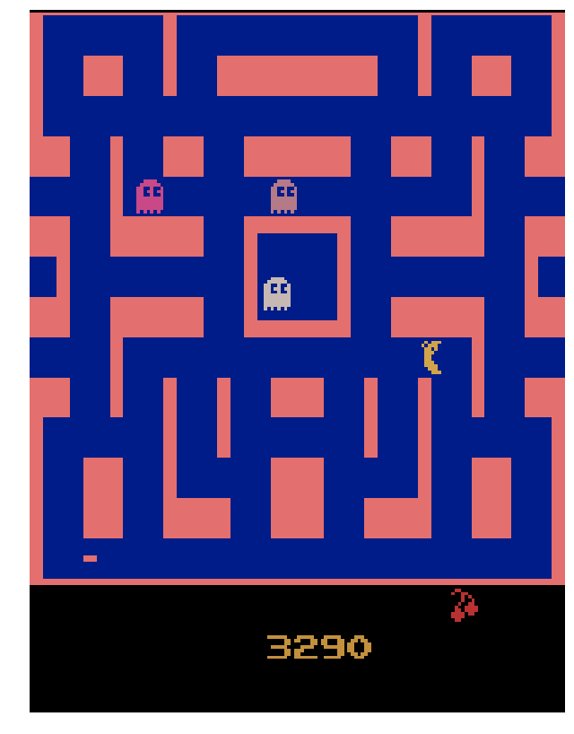
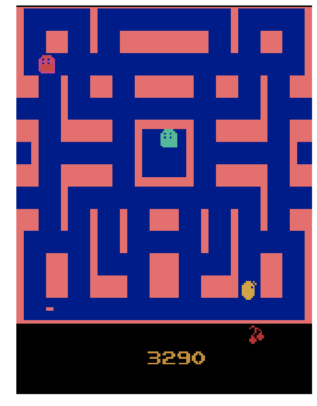
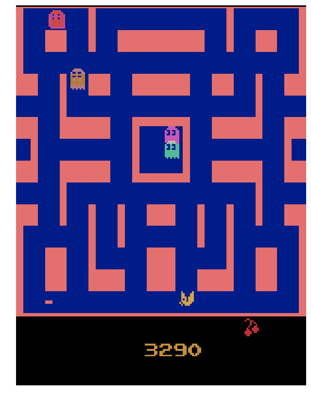
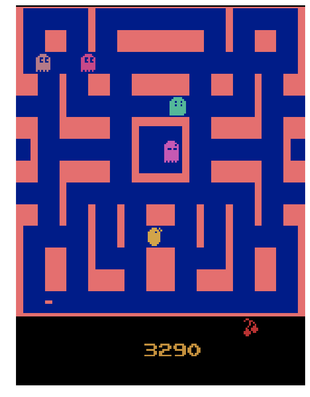
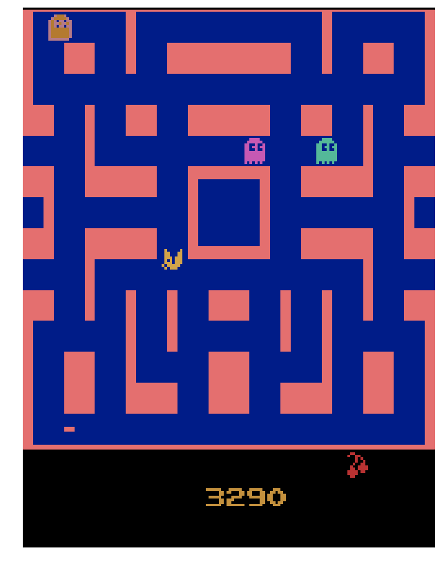
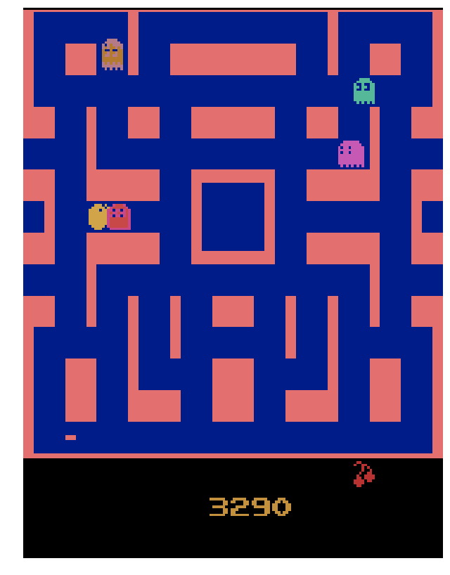
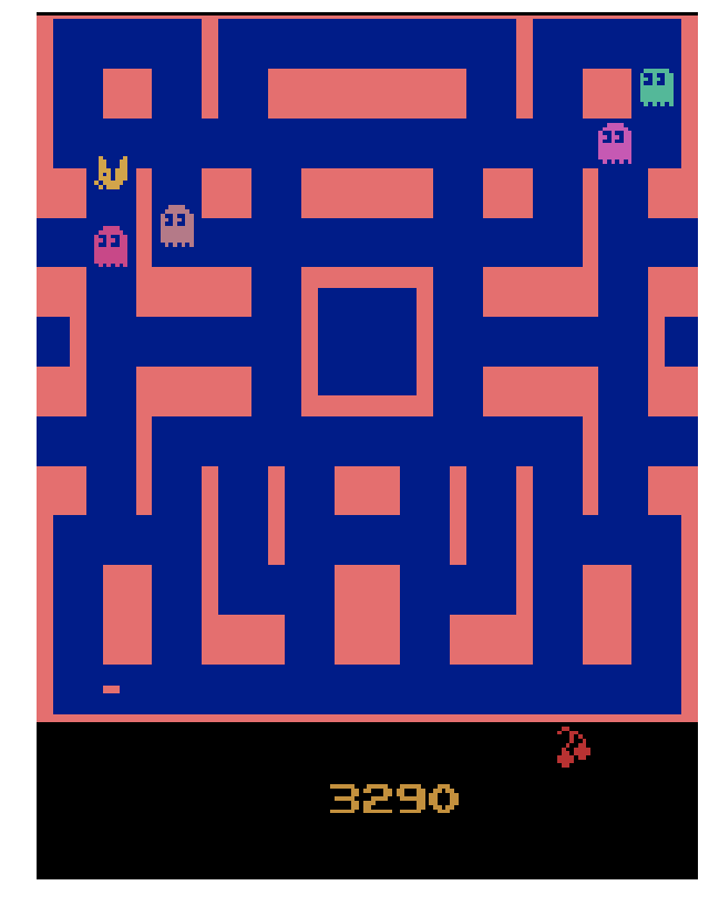
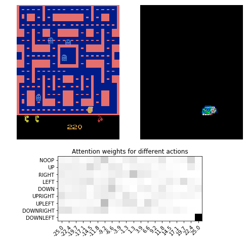
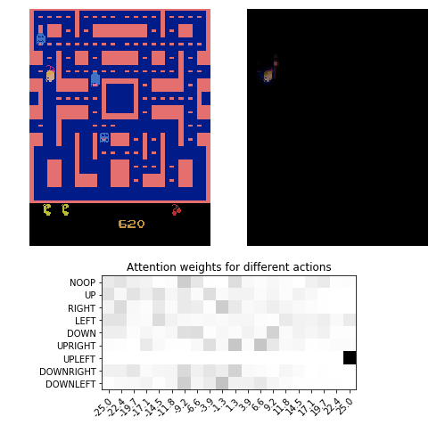
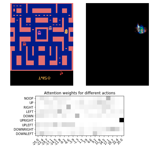
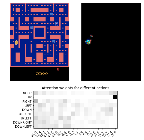
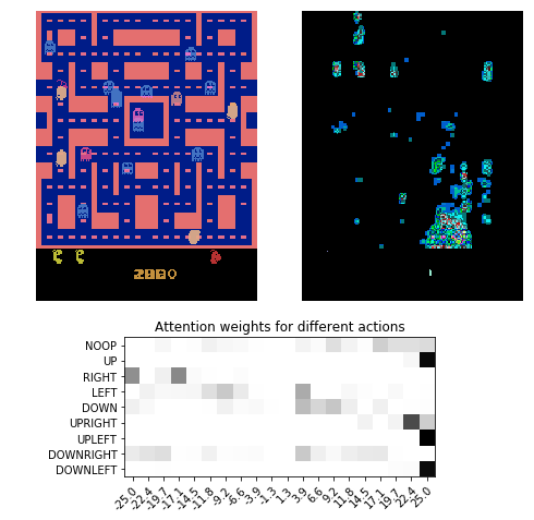
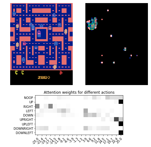
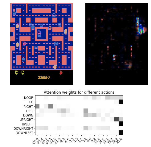
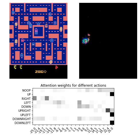
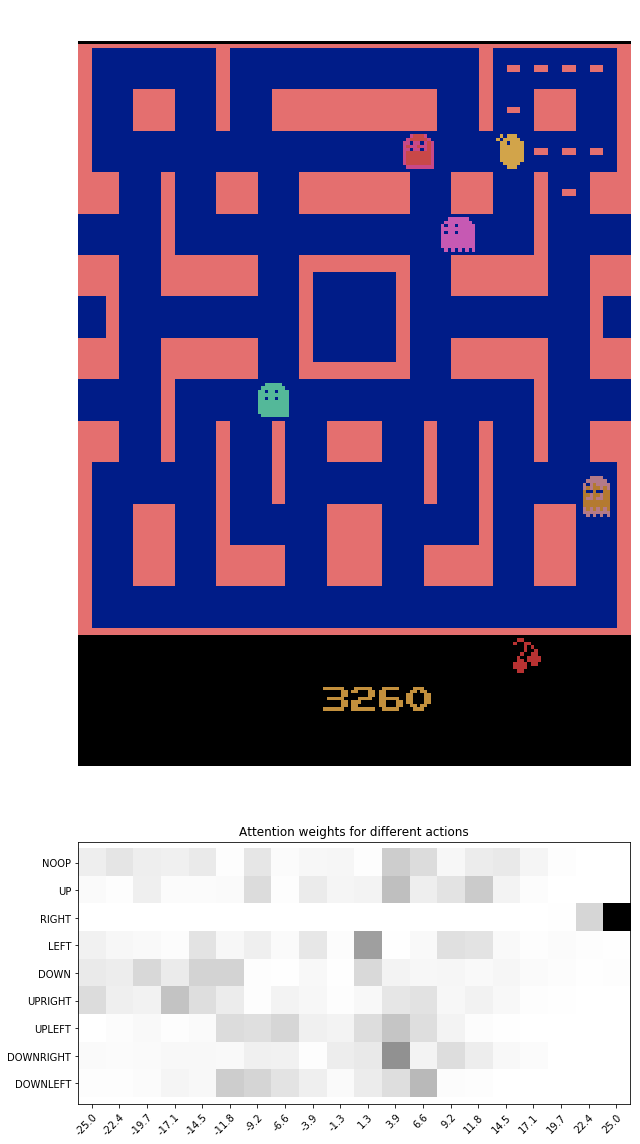
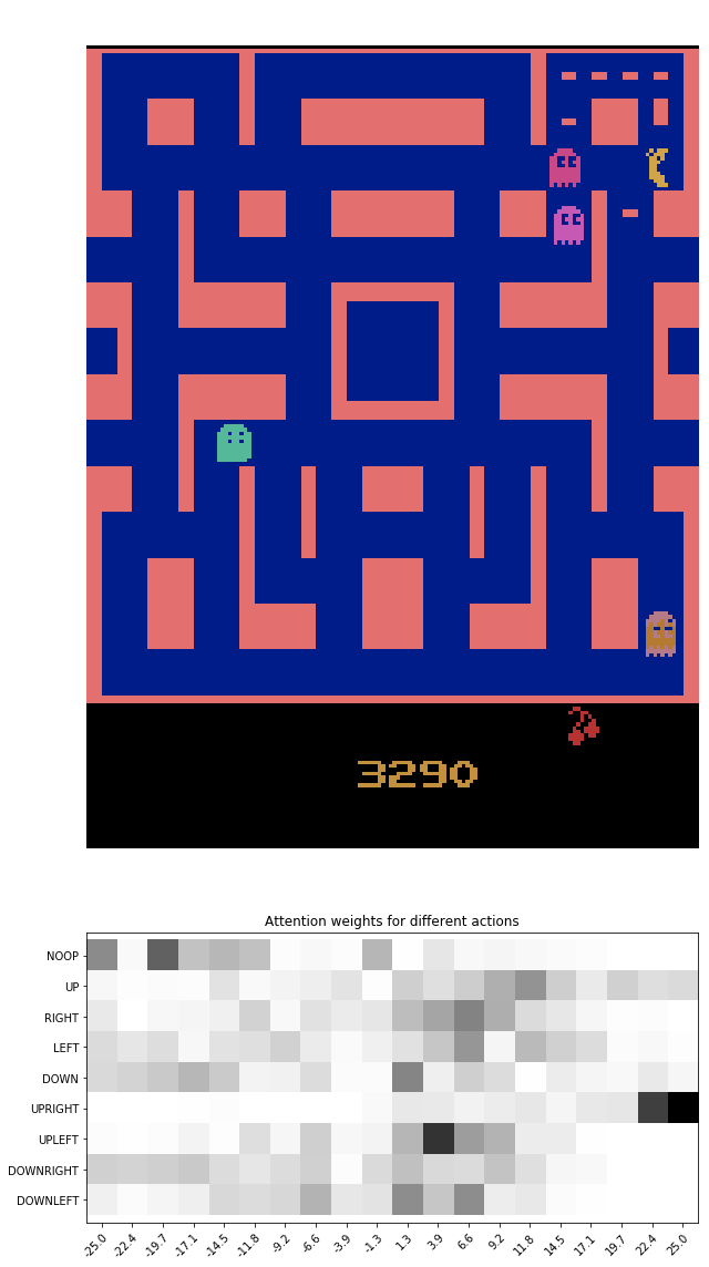
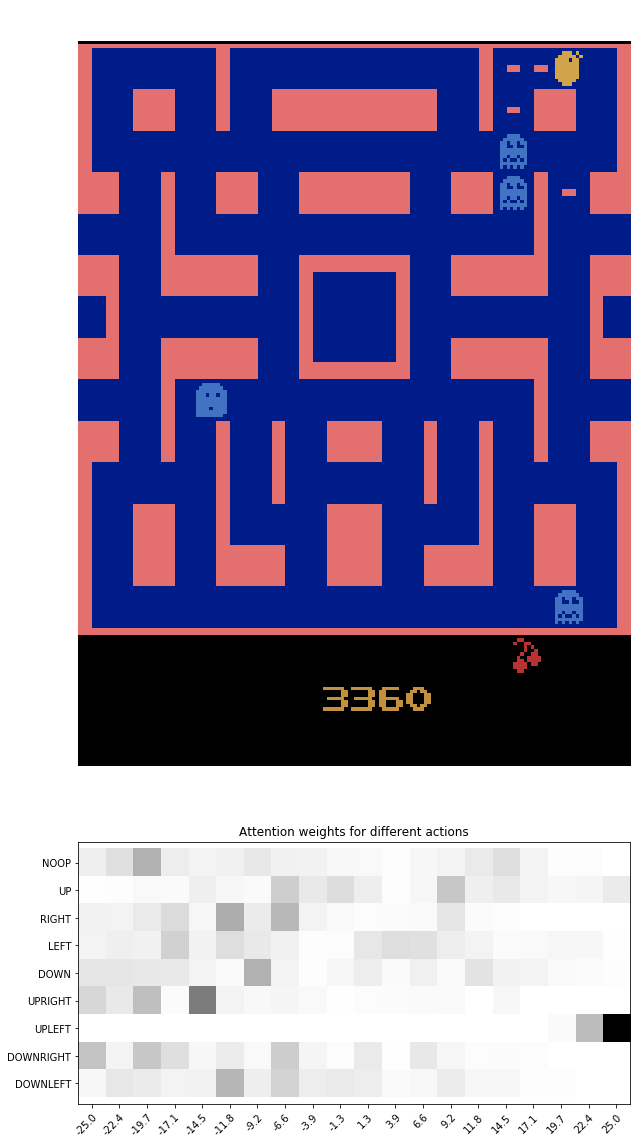
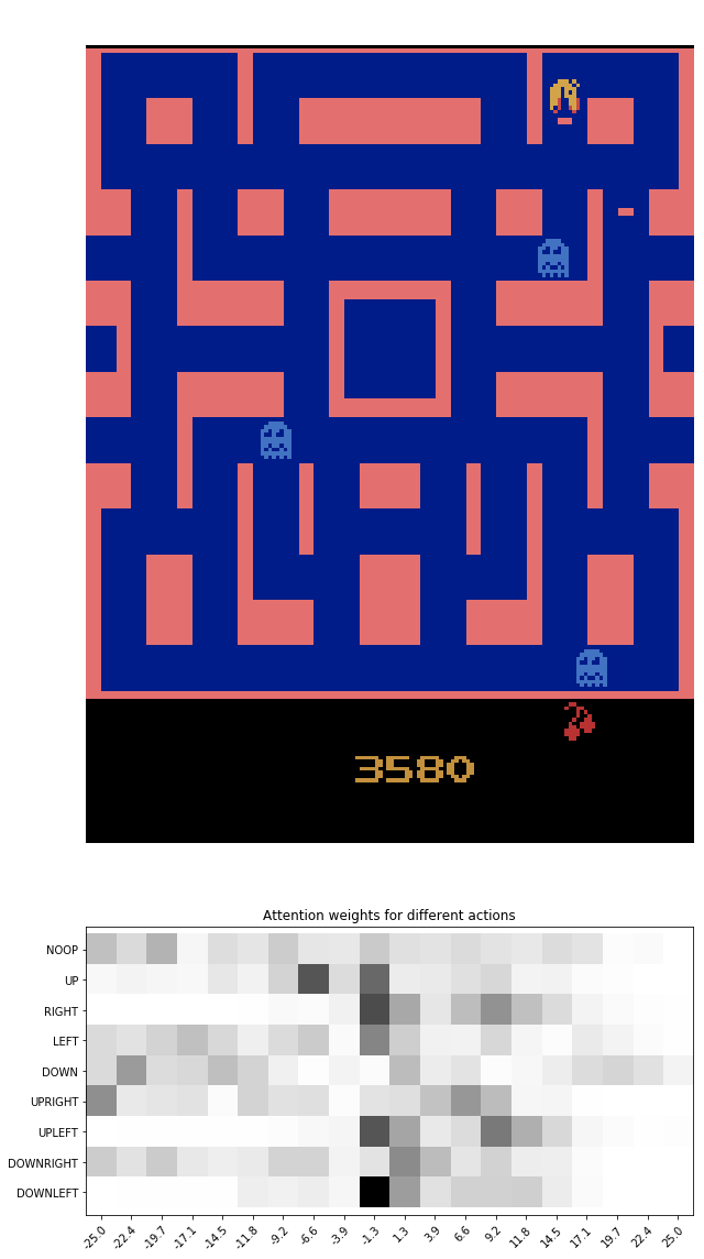
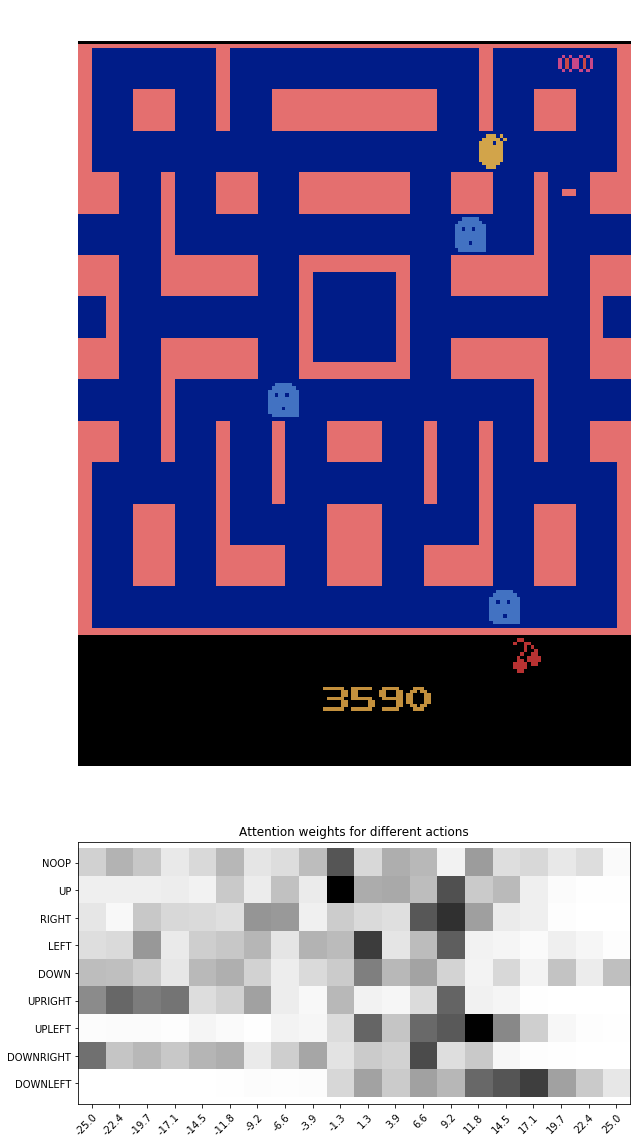
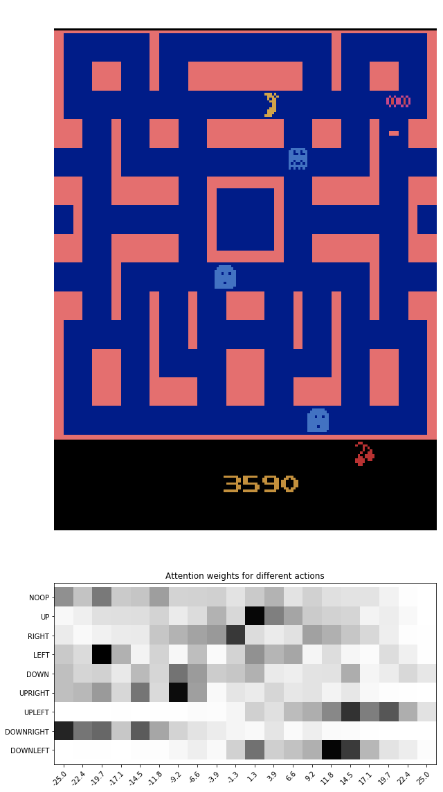
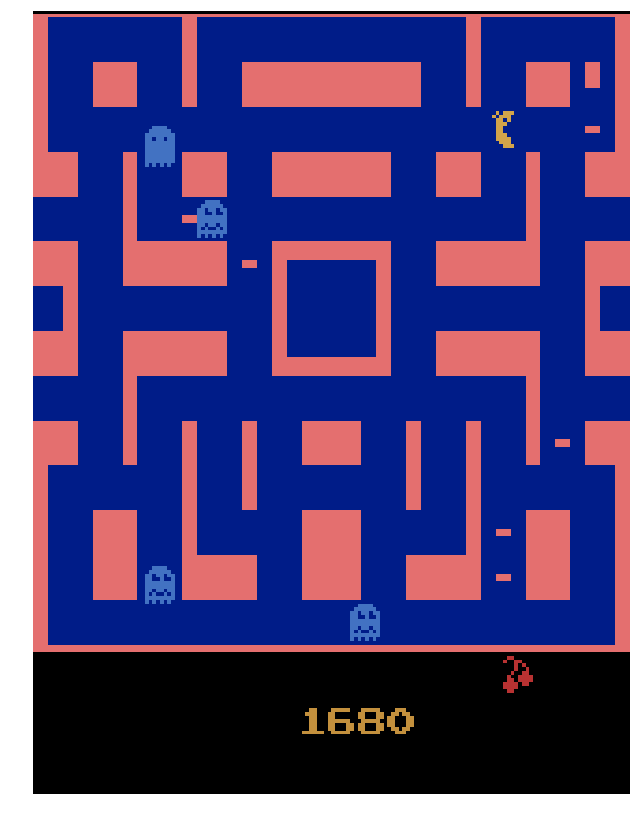
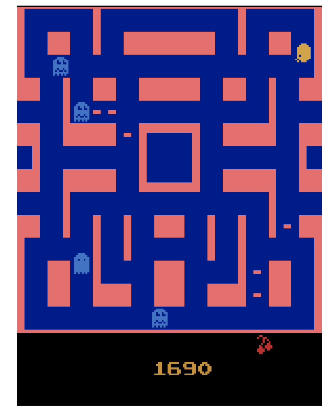
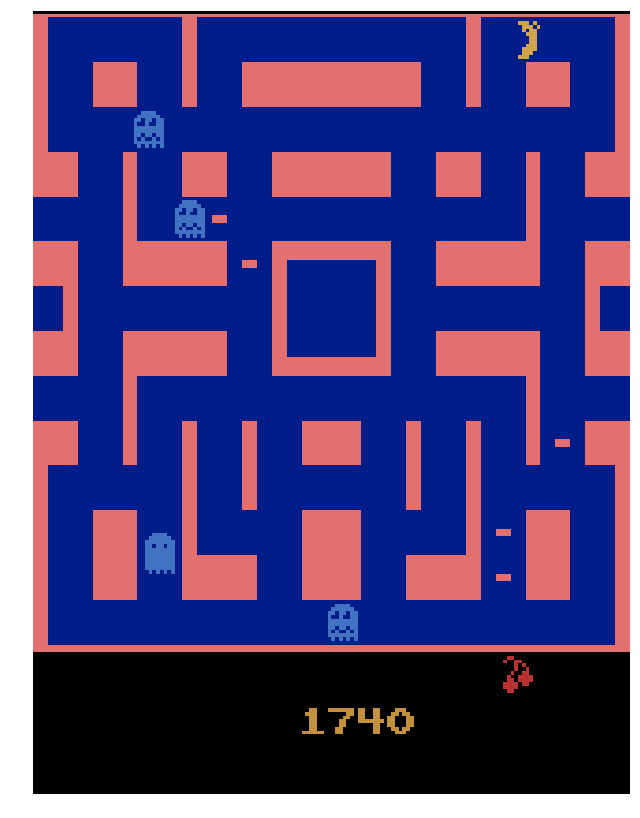
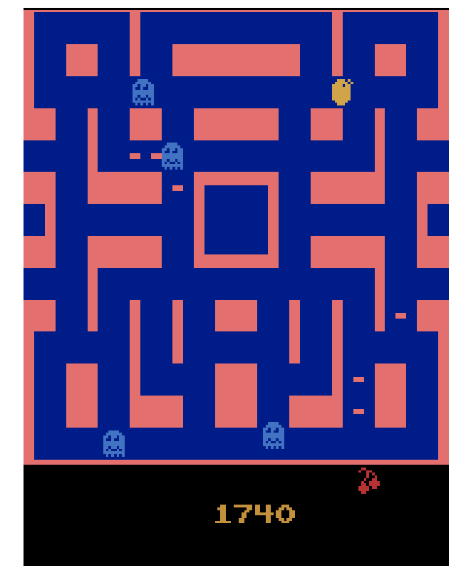
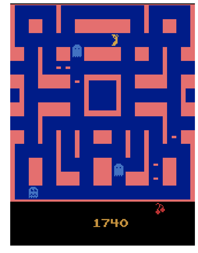
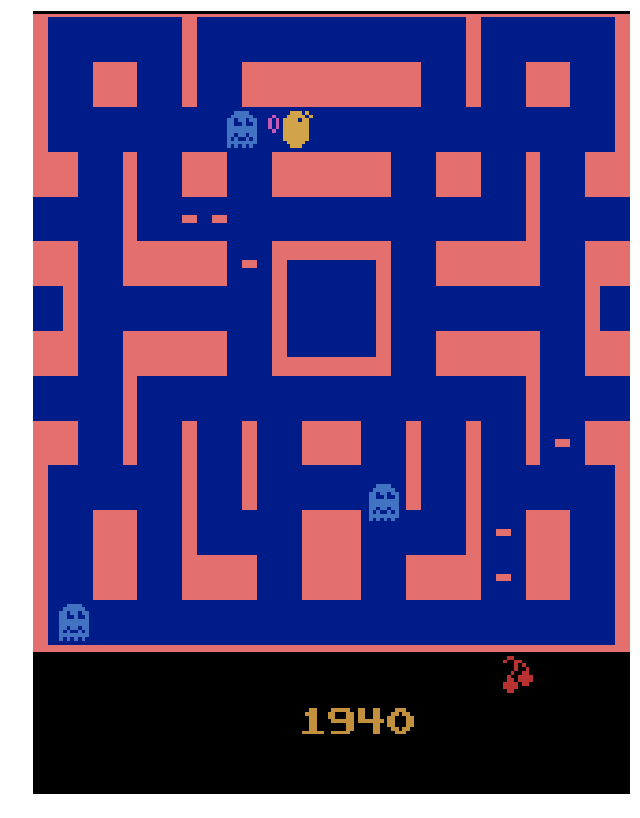
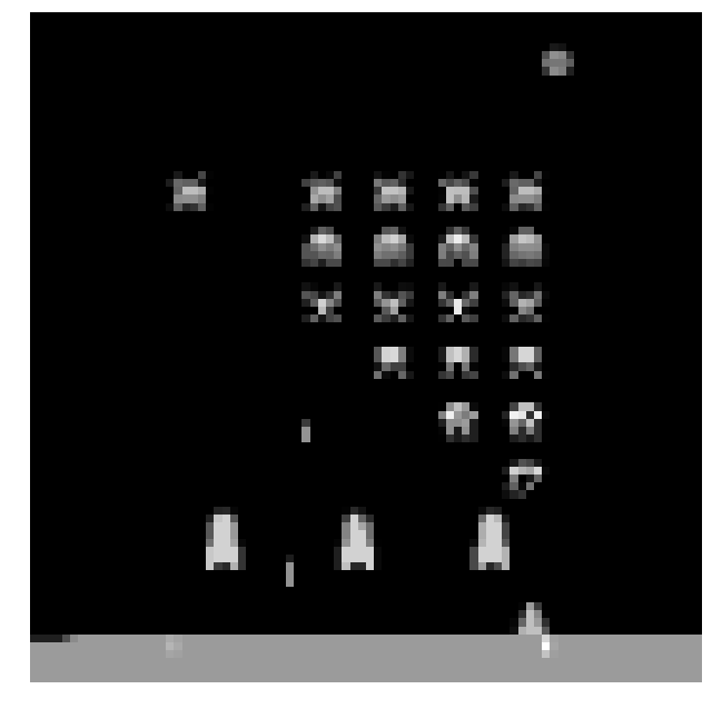
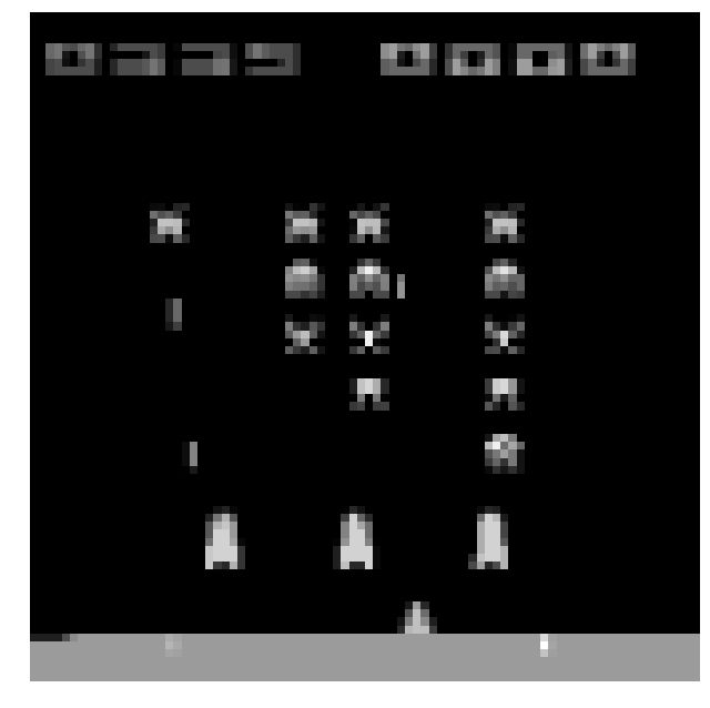
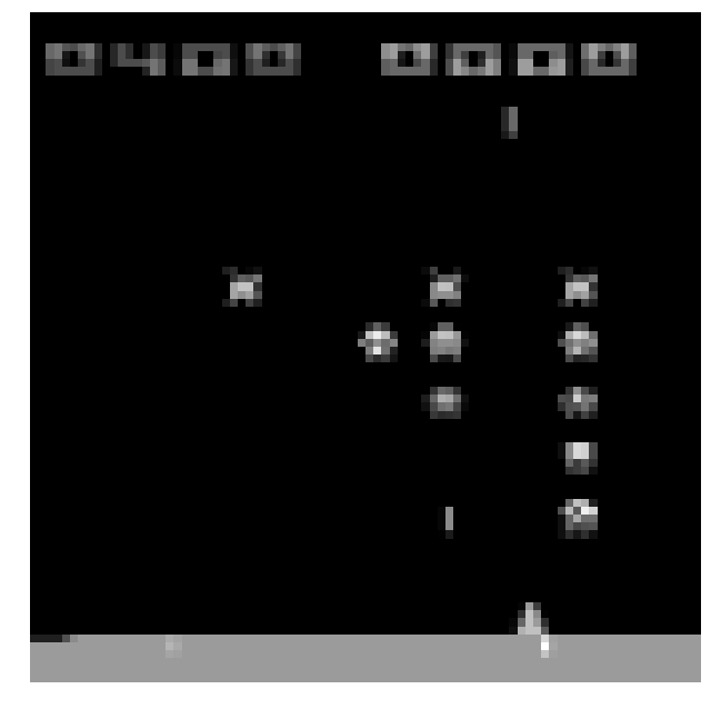
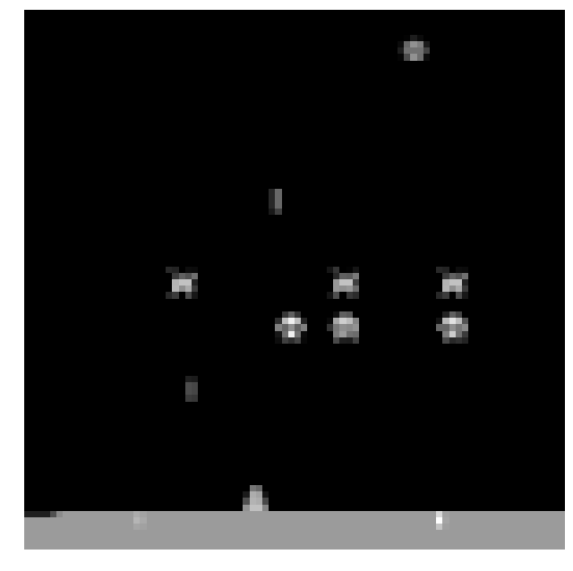
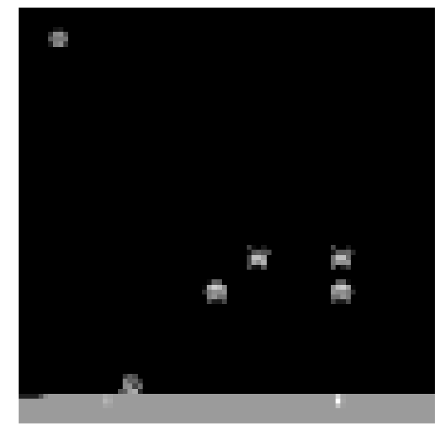
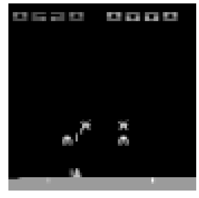
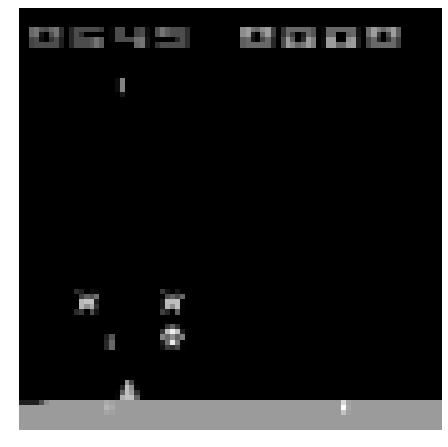
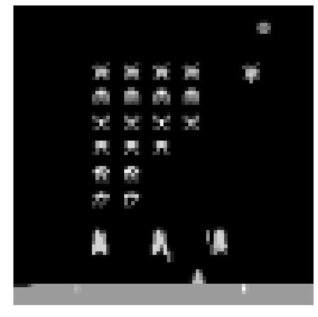
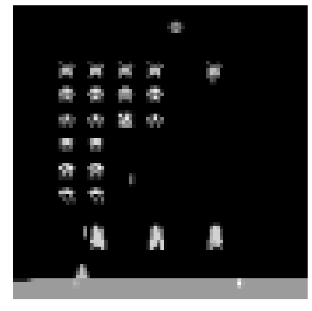
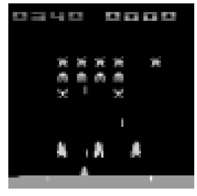
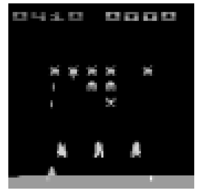
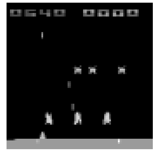
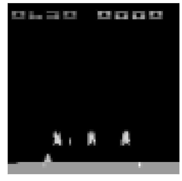
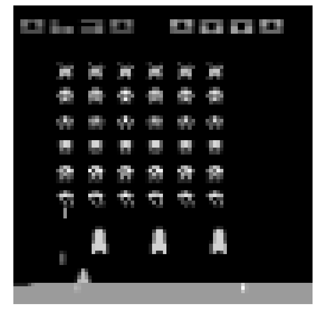
Looking at the visualizations and rollouts of a fully trained agent, we hand-craft a few out-of-sample environment states to examine the agent’s generalization behavior. For example, in MsPacman, since visualizations suggest that the agent may be memorizing pacman’s positions (also maybe ghosts and other objects), we simply add an extra pellet adjacent to a trajectory seen during training (Figure 8(a)). The agent does not clear the additional pellet and simply continues to execute actions performed during training (Figure 8(b)). Most importantly, the agent is extremely confident in taking actions initially (seen in attention maps Figure 8(a)) which suggest that the extra pellet was probably not even captured by the embeddings. Similarly, in case of SpaceInvaders, the agent has a strong bias towards shooting from the leftmost-end (seen in Figure 4). This helps in clearing the triangle like shape and moving to the next level (Figure 8(d)). However, when triangular positions of spaceships are inverted, the agent repeats the same strategy of trying to shoot from left and fails to clear ships (Figure 8(c)). These examples indicate that the features extracted by the convolutional channels seem to be shallow. The agent does not really model interactions between objects. For example in MsPacman, after observing 10M frames, it does not know general relationships between pacman and pellet or ghosts. Even if optimal Q-values were known, there is no incentive for the network to model these higher order dependencies when it can work with situational features extracted from finite training examples. (?) also report similar results on simple mazes where an agent trained on insufficient environments tends to repeat training trajectories on unseen mazes.
Sensitivity to hyperparameters
I-DQN’s objective function introduces four hyperparameters for weighting the different loss components (: for bellman error, : distributional error, : reconstruction error and : diversity error). The diversity error forces attention over multiple keys (examples for and are shown in the supplementary material). In general, we found the values , , , to work well across games (detailed list of hyperparameters and their values is reported in the supplementary material). We ran experiments for different settings of , and keeping constant on Ms Pacman (averaged over 3 trials). In general, increasing (coefficient on reconstruction error) to and yields visually better quality reconstructions but poorer scores- and respectively (drop by %). Increasing also drops the score and yields poor reconstructions (sometimes without the objects of the game which loses interpretability) but converges quite quickly (, drop by %). Out of (bellman loss) and (distributional loss), seems to play a more important in reaching higher scores compared to [, score: ; , , score: ]. So, the setting , , , seems to find the right balance between the q-value learning losses and regularizing losses. For the exploration factor, we tried a few different values and it did not have a significant effect on the scores.
Conclusion
In this paper, we propose an interpretable deep Q-network model (i-DQN) that can be studied using a variety of tools including the usual saliency maps, attention maps and reconstructions of key embeddings that attempt to provide global explanations of the model’s behavior. We also show that the uncertainty in soft cluster assignment can be used to drive exploration effectively and achieve high training rewards comparable to other models. Although the reconstructions do not explain the agent’s decisions perfectly, they provide a better insight into the kind of features extracted by convolutional layers. This can be used to design interesting adversarial examples with slight modifications to the state of the environment where the agent fails to adapt and instead repeats action sequences that were performed during training. This is the general problem of overfitting in machine learning but is more acute in the case of reinforcement learning because the process of collecting training examples depends largely on the agent’s biases (exploration). There are many interesting directions for future work. For example, we know that the reconstruction method largely affects the visualizations and other methods such as generative adversarial networks (GANs) (?) can model latent spaces more smoothly and could generalize better to unseen embeddings. Another direction is to see if we can automatically detect the biases learned by the agent and design meaningful adversarial examples instead of manually crafting test cases.
Acknowledgments
This work was funded by awards AFOSR FA9550-15-1-0442 and NSF IIS- 1724222.
References
- [Arulkumaran et al. 2017] Arulkumaran, K.; Deisenroth, M. P.; Brundage, M.; and Bharath, A. A. 2017. A brief survey of deep reinforcement learning. arXiv preprint arXiv:1708.05866.
- [Bellemare et al. 2016] Bellemare, M.; Srinivasan, S.; Ostrovski, G.; Schaul, T.; Saxton, D.; and Munos, R. 2016. Unifying count-based exploration and intrinsic motivation. In Advances in Neural Information Processing Systems, 1471–1479.
- [Bellemare, Dabney, and Munos 2017] Bellemare, M. G.; Dabney, W.; and Munos, R. 2017. A distributional perspective on reinforcement learning. arXiv preprint arXiv:1707.06887.
- [Brockman et al. 2016] Brockman, G.; Cheung, V.; Pettersson, L.; Schneider, J.; Schulman, J.; Tang, J.; and Zaremba, W. 2016. Openai gym.
- [Chang et al. 2017] Chang, J.; Wang, L.; Meng, G.; Xiang, S.; and Pan, C. 2017. Deep adaptive image clustering. In 2017 IEEE International Conference on Computer Vision (ICCV), 5880–5888. IEEE.
- [Chen et al. 2018] Chen, R. Y.; Sidor, S.; Abbeel, P.; and Schulman, J. 2018. Ucb exploration via q-ensembles.
- [Choi et al. 2017] Choi, E.; Hewlett, D.; Uszkoreit, J.; Polosukhin, I.; Lacoste, A.; and Berant, J. 2017. Coarse-to-fine question answering for long documents. In Proceedings of the 55th Annual Meeting of the Association for Computational Linguistics (Volume 1: Long Papers), volume 1, 209–220.
- [Dosovitskiy and Brox 2016] Dosovitskiy, A., and Brox, T. 2016. Inverting visual representations with convolutional networks. In Proceedings of the IEEE Conference on Computer Vision and Pattern Recognition, 4829–4837.
- [Fortunato et al. 2017] Fortunato, M.; Azar, M. G.; Piot, B.; Menick, J.; Osband, I.; Graves, A.; Mnih, V.; Munos, R.; Hassabis, D.; Pietquin, O.; et al. 2017. Noisy networks for exploration. arXiv preprint arXiv:1706.10295.
- [Goodfellow et al. 2014] Goodfellow, I.; Pouget-Abadie, J.; Mirza, M.; Xu, B.; Warde-Farley, D.; Ozair, S.; Courville, A.; and Bengio, Y. 2014. Generative adversarial nets. In Advances in neural information processing systems, 2672–2680.
- [Greydanus et al. 2017] Greydanus, S.; Koul, A.; Dodge, J.; and Fern, A. 2017. Visualizing and understanding atari agents. arXiv preprint arXiv:1711.00138.
- [Henderson et al. 2017] Henderson, P.; Islam, R.; Bachman, P.; Pineau, J.; Precup, D.; and Meger, D. 2017. Deep reinforcement learning that matters. arXiv preprint arXiv:1709.06560.
- [Hessel et al. 2017] Hessel, M.; Modayil, J.; Van Hasselt, H.; Schaul, T.; Ostrovski, G.; Dabney, W.; Horgan, D.; Piot, B.; Azar, M.; and Silver, D. 2017. Rainbow: Combining improvements in deep reinforcement learning. arXiv preprint arXiv:1710.02298.
- [Huang et al. 2017] Huang, S.; Papernot, N.; Goodfellow, I.; Duan, Y.; and Abbeel, P. 2017. Adversarial attacks on neural network policies. arXiv preprint arXiv:1702.02284.
- [Iyer et al. 2018] Iyer, R.; Li, Y.; Li, H.; Lewis, M.; Sundar, R.; and Sycara, K. 2018. Transparency and explanation in deep reinforcement learning neural networks.
- [Kindermans et al. 2017] Kindermans, P.-J.; Hooker, S.; Adebayo, J.; Alber, M.; Schütt, K. T.; Dähne, S.; Erhan, D.; and Kim, B. 2017. The (un) reliability of saliency methods. arXiv preprint arXiv:1711.00867.
- [Kraska et al. 2018] Kraska, T.; Beutel, A.; Chi, E. H.; Dean, J.; and Polyzotis, N. 2018. The case for learned index structures. In Proceedings of the 2018 International Conference on Management of Data, 489–504. ACM.
- [Levine et al. 2016] Levine, S.; Finn, C.; Darrell, T.; and Abbeel, P. 2016. End-to-end training of deep visuomotor policies. The Journal of Machine Learning Research 17(1):1334–1373.
- [Li, Sycara, and Iyer 2017] Li, Y.; Sycara, K. P.; and Iyer, R. 2017. Object-sensitive deep reinforcement learning. In GCAI 2017, 3rd Global Conference on Artificial Intelligence, Miami, FL, USA, 18-22 October 2017., 20–35.
- [Lin et al. 2017] Lin, Z.; Feng, M.; Santos, C. N. d.; Yu, M.; Xiang, B.; Zhou, B.; and Bengio, Y. 2017. A structured self-attentive sentence embedding. arXiv preprint arXiv:1703.03130.
- [Lipton 2016] Lipton, Z. C. 2016. The mythos of model interpretability. arXiv preprint arXiv:1606.03490.
- [Mnih et al. 2015] Mnih, V.; Kavukcuoglu, K.; Silver, D.; Rusu, A. A.; Veness, J.; Bellemare, M. G.; Graves, A.; Riedmiller, M.; Fidjeland, A. K.; Ostrovski, G.; et al. 2015. Human-level control through deep reinforcement learning. Nature 518(7540):529.
- [Oh et al. 2015] Oh, J.; Guo, X.; Lee, H.; Lewis, R. L.; and Singh, S. 2015. Action-conditional video prediction using deep networks in atari games. In Advances in Neural Information Processing Systems, 2863–2871.
- [Osband et al. 2016] Osband, I.; Blundell, C.; Pritzel, A.; and Van Roy, B. 2016. Deep exploration via bootstrapped dqn. In Advances in neural information processing systems, 4026–4034.
- [Ostrovski et al. 2017] Ostrovski, G.; Bellemare, M. G.; Oord, A. v. d.; and Munos, R. 2017. Count-based exploration with neural density models. arXiv preprint arXiv:1703.01310.
- [Pritzel et al. 2017] Pritzel, A.; Uria, B.; Srinivasan, S.; Puigdomenech, A.; Vinyals, O.; Hassabis, D.; Wierstra, D.; and Blundell, C. 2017. Neural episodic control. arXiv preprint arXiv:1703.01988.
- [Silver et al. 2017] Silver, D.; Hubert, T.; Schrittwieser, J.; Antonoglou, I.; Lai, M.; Guez, A.; Lanctot, M.; Sifre, L.; Kumaran, D.; Graepel, T.; et al. 2017. Mastering chess and shogi by self-play with a general reinforcement learning algorithm. arXiv preprint arXiv:1712.01815.
- [Van Hasselt, Guez, and Silver 2016] Van Hasselt, H.; Guez, A.; and Silver, D. 2016. Deep reinforcement learning with double q-learning.
- [Verma et al. 2018] Verma, A.; Murali, V.; Singh, R.; Kohli, P.; and Chaudhuri, S. 2018. Programmatically interpretable reinforcement learning. arXiv preprint arXiv:1804.02477.
- [Williams, Asadi, and Zweig 2017] Williams, J. D.; Asadi, K.; and Zweig, G. 2017. Hybrid code networks: practical and efficient end-to-end dialog control with supervised and reinforcement learning. arXiv preprint arXiv:1702.03274.
- [Xie, Girshick, and Farhadi 2016] Xie, J.; Girshick, R.; and Farhadi, A. 2016. Unsupervised deep embedding for clustering analysis. In International conference on machine learning, 478–487.
- [Zahavy, Ben-Zrihem, and Mannor 2016] Zahavy, T.; Ben-Zrihem, N.; and Mannor, S. 2016. Graying the black box: Understanding dqns. In International Conference on Machine Learning, 1899–1908.
- [Zhang and Zhu 2018] Zhang, Q.-s., and Zhu, S.-C. 2018. Visual interpretability for deep learning: a survey. Frontiers of Information Technology & Electronic Engineering 19(1):27–39.
- [Zhang, Ballas, and Pineau 2018] Zhang, A.; Ballas, N.; and Pineau, J. 2018. A dissection of overfitting and generalization in continuous reinforcement learning. arXiv preprint arXiv:1806.07937.
- [Zhang et al. 2018] Zhang, C.; Vinyals, O.; Munos, R.; and Bengio, S. 2018. A study on overfitting in deep reinforcement learning. arXiv preprint arXiv:1804.06893.
Supplemental Material
In this supplemental material, we include details of the experiment setup, hyperparameters and experiment results in terms of training curves. We present additional visualizations for the other games discussed in the paper and a few more adversarial examples for MsPacman. We also include an ablation study on the effect of the different loss functions.
Experimental Setup
The i-DQN training algorithm is described in Algorithm 1 (including the directed exploration strategy and visualization step). As discussed in the paper, the i-DQN model attempts to minimize a weighted linear combination of multiple losses.
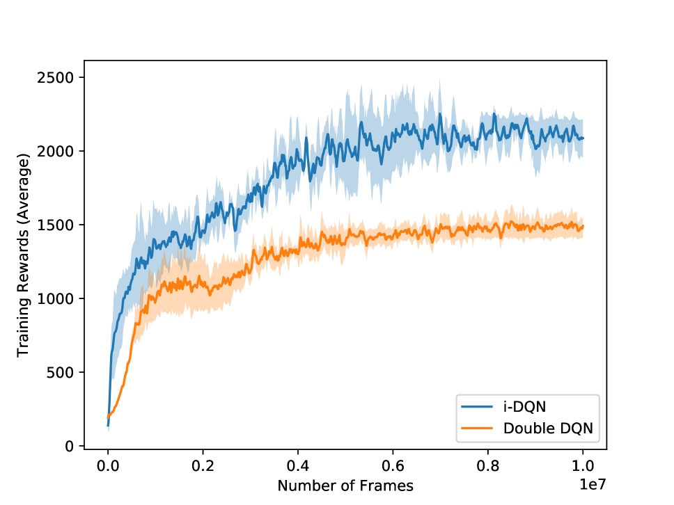
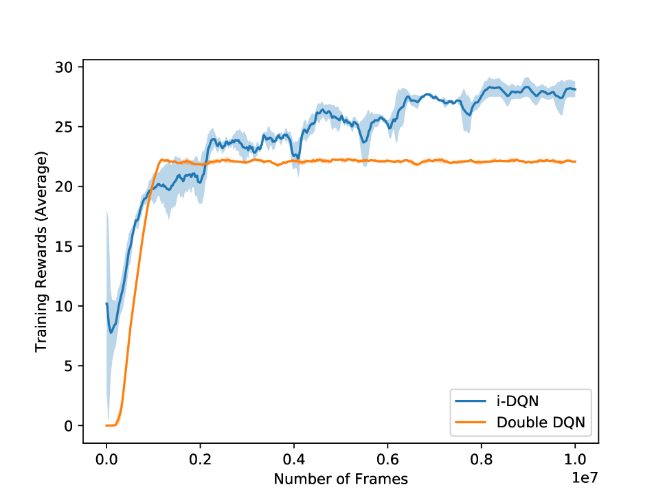
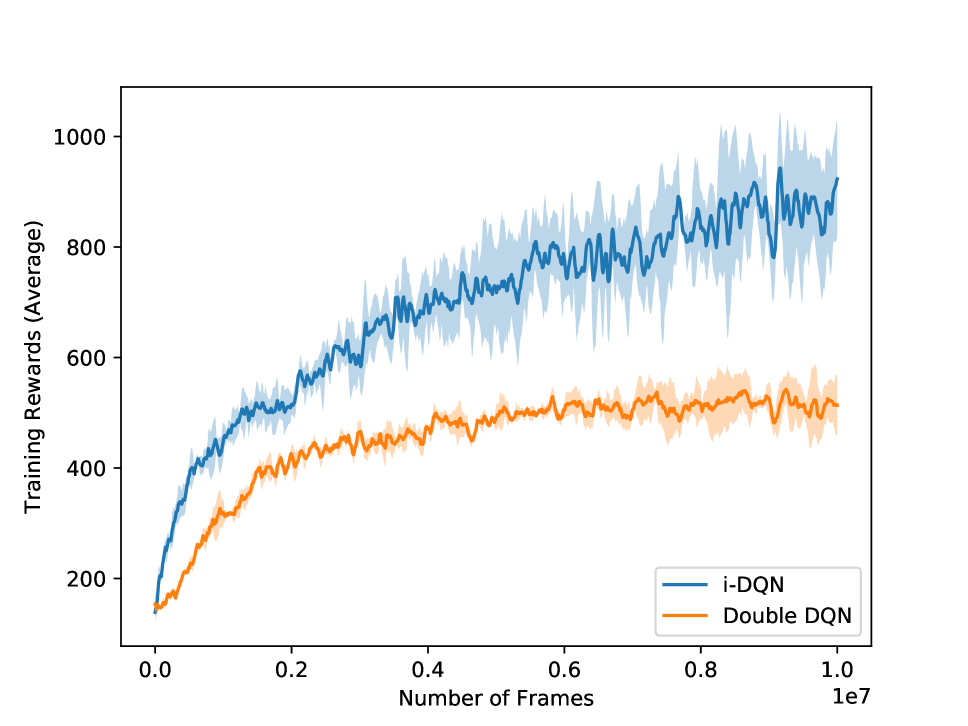
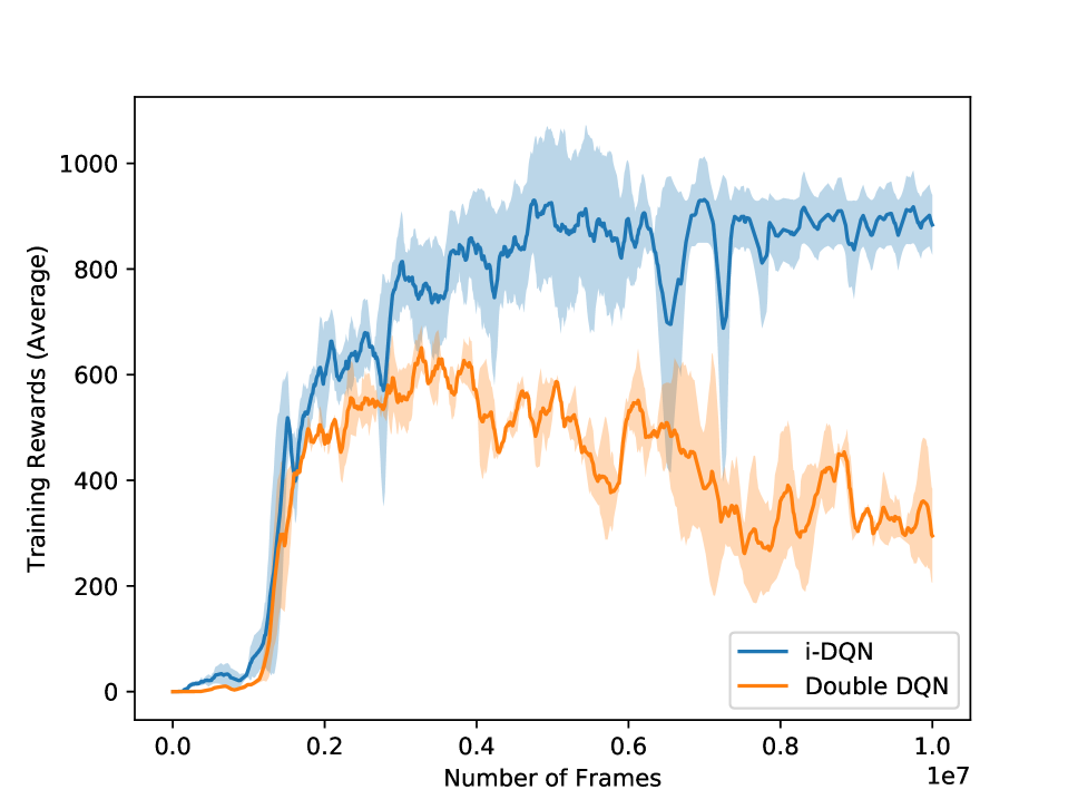
Table 3 lists all the hyperparameters (including network architecture), values and their description. Most of the training procedure and hyperparameter values are similar to the settings in (?) and (?). Figure 9 shows the training curves for i-DQN and double DQN models over three random seeds for eight different Atari environments- Alien, Freeway, Frostbite, Gravitar, MsPacman, Qbert, SpaceInvaders, and Venture. The results reported in the paper are averaged over the best results for individual runs for each seed. Although training i-DQN is slow, the directed exploration strategy helps to quickly reach scores competitive with the state-of-the-art deep Q-learning based models.
| Hyperparameter | Value | Description |
|---|---|---|
| Number of Keys per Action () | 20 | Total keys in key-value store for actions |
| Range of Values , | The range from which the values of key-value store are sampled | |
| Exploration Factor | Controls the ucb style action selection using confidence intervals | |
| Embedding Size | 256 | Dimensions of latent space where keys and state embeddings lie |
| Network Channels | Convolution layers (Channels, Filter, Stride) | |
| Network Activations | ReLU | |
| Discount Factor | 0.99 | |
| Batch Size | 32 | |
| Optimizer | Adam | learning rate, beta1, beta2, weight decay |
| Gradient Clipping | 10 | Using gradient norm |
| Replay Buffer Size | 10K | |
| Training Frequency | Every 4 steps | |
| Target Network Sync Frequency | 1000 | Fully replaced with weights from source/training network |
| Frame Preprocessing | Standard | Grayscaling, Downsampling (84, 84), Frames stacked: 4, Repeat Actions: 4 |
| Reward Clipping | No | |
| Loss Factors | , , , | The weights on each loss function |
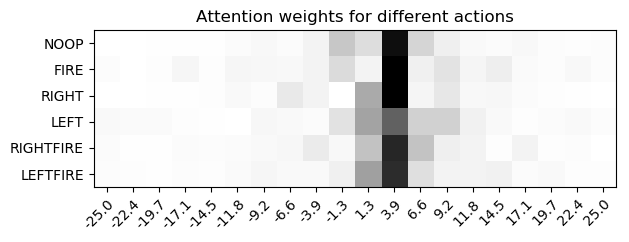
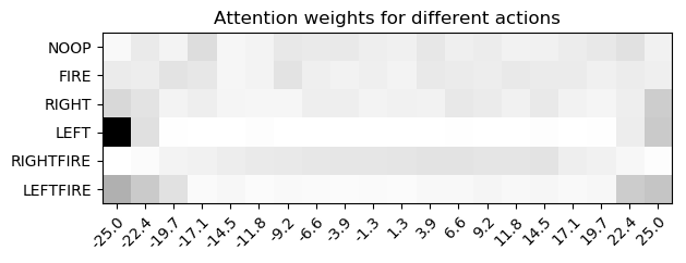
Attention Maps: During training, the i-DQN model learns to attend over keys in the key-value store using a dot-product attention.
We can visualize these weights in terms of attention heat-maps where each row is a distribution over Q-values (because of the softmax) for a particular action. Darker cells imply higher attention weights, for example in Figure 10(c), the agent expects a negative return of -25 with very high probability for action ’Left’.
Saliency Maps: They usually highlight the most sensitive regions around the input that can cause the neural network to change its predictions. Following (?), we define saliency maps as follows,
defines the perturbed image for state at pixel location , is the saliency mask usually a Gaussian centered at defining the sensitive region, is a Gaussian blur of and denotes the sensitivity of to pixel location .
Analysing Loss Functions
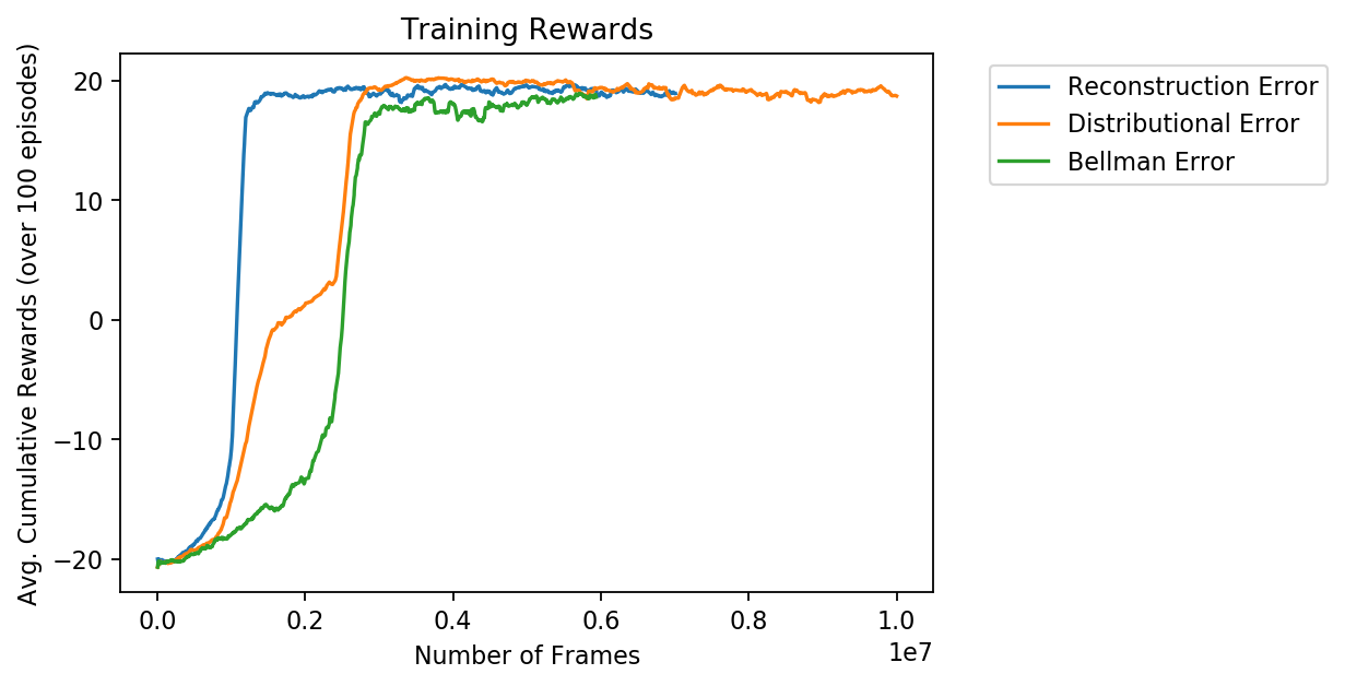
Figure 10(a) shows the effect of different loss functions. We keep the diversity error constant and incrementally add each of the loss functions. Figure 10(b) and Figure 10(c) show the effect of the diversity loss. Without the diversity loss, the network can learn to attend over a small set of the keys for each action. However, the diversity loss encourages attention across elements in a batch to be diverse and ideally, the attention weights should concentrate on a single key (because of l- and l- norm constraints) but concentrate over very few keys in practice .
|
|




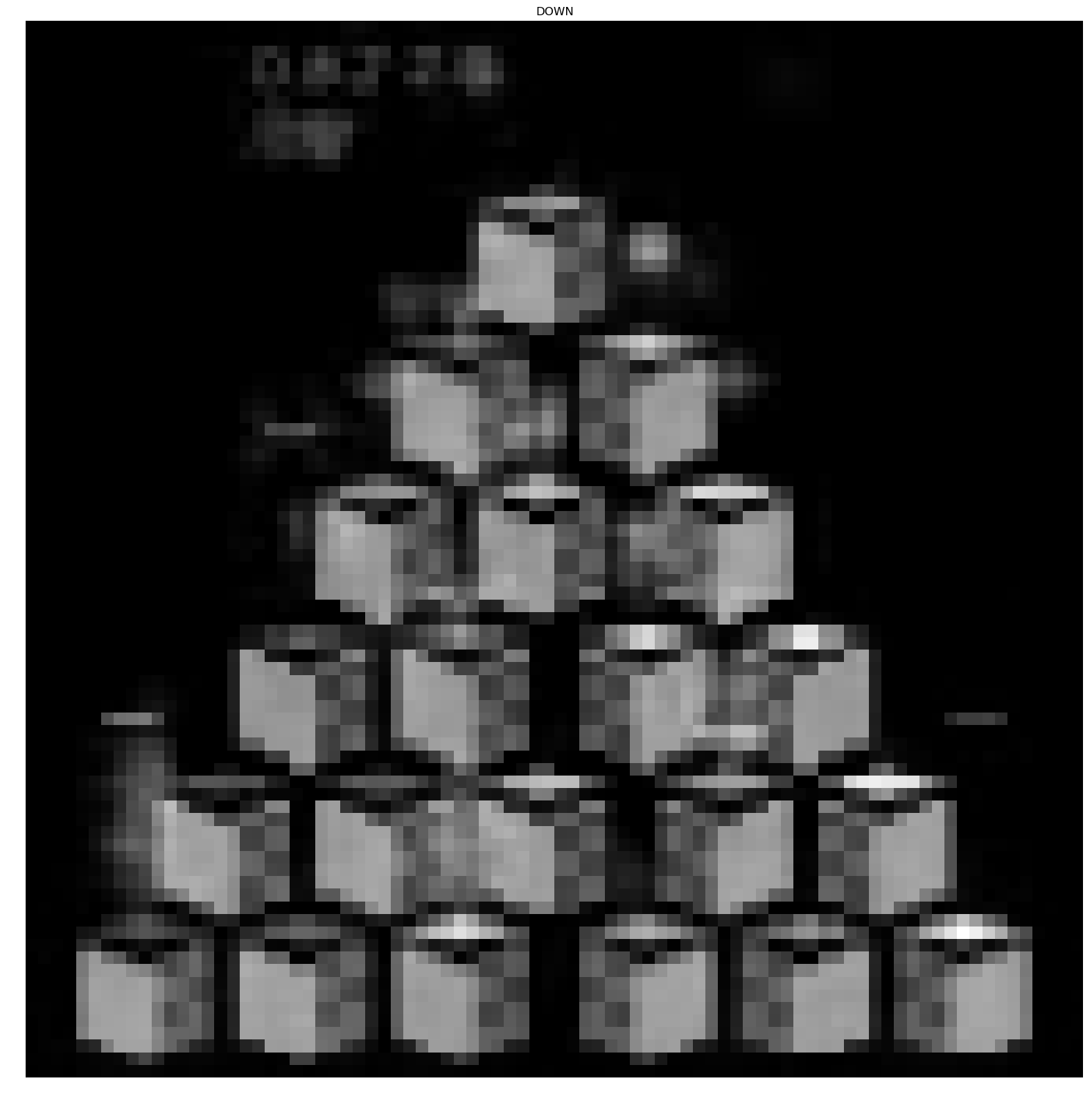
s
Inversion of Keys
Figures 4, 12 show the reconstructed images by inverting keys in MsPacman (some of these have been discussed in the paper). Figures 14(a), 14(b) show the reconstructed images by inverting keys in Pong and Qbert. Most of these images are noisy, especially the ones in gray-scale but seem to indicate configurations of different objects in the game. Figure 19 shows the reconstructions by interpolating in the hidden space starting from a key embedding and moving towards a specific training state. We see that most of the hidden space can be reconstructed but the information about shapes and colors of the objects is not always clear while reconstructing the key embeddings.
Adversarial Examples for MsPacman
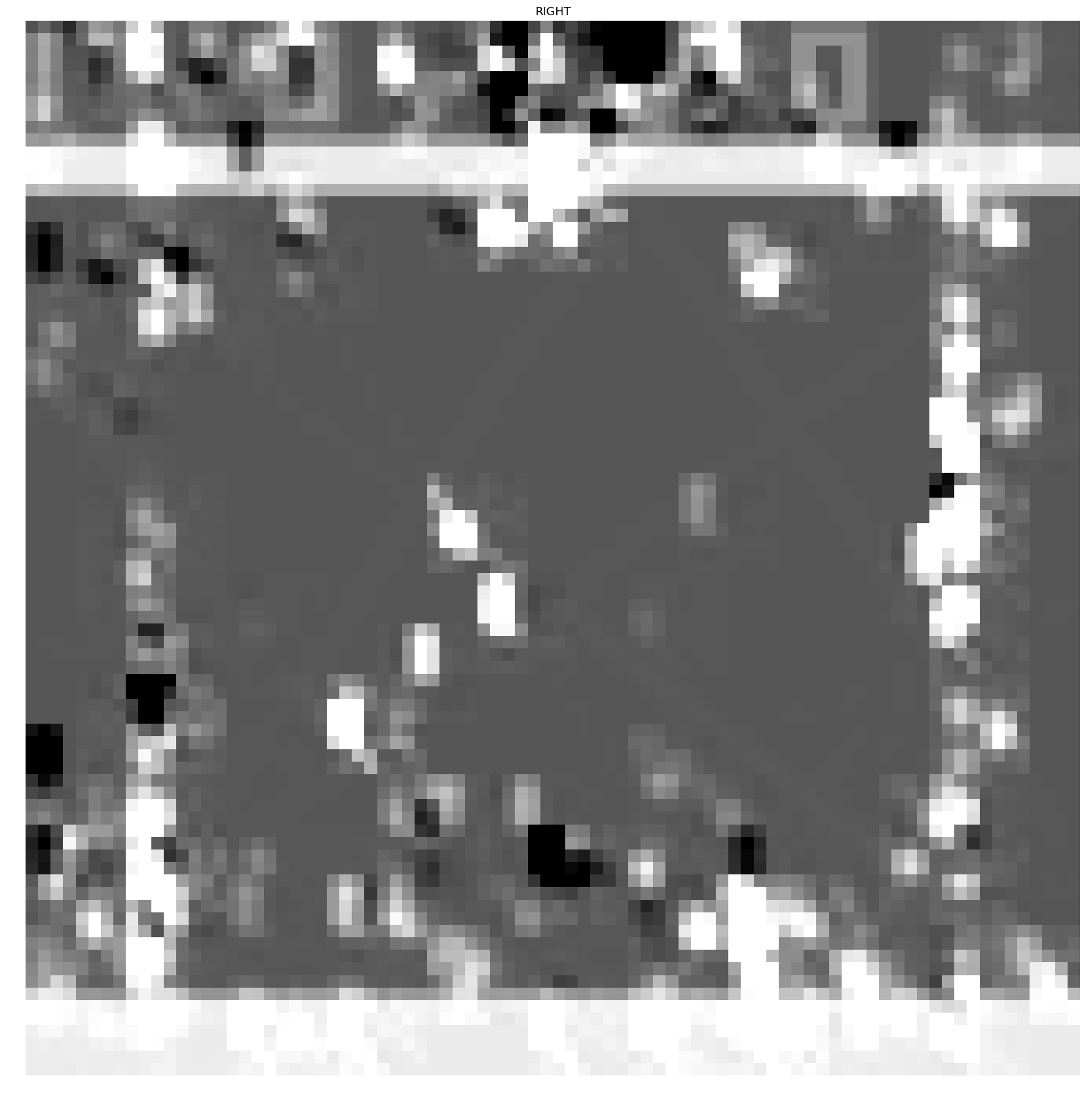
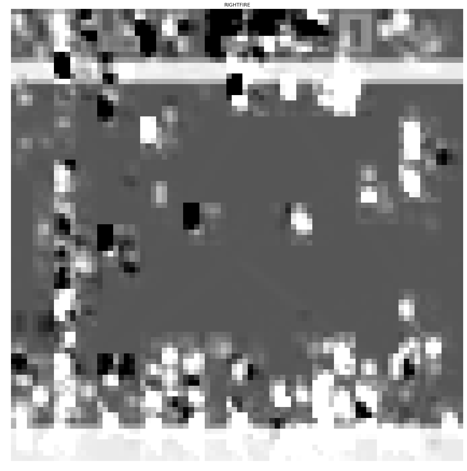
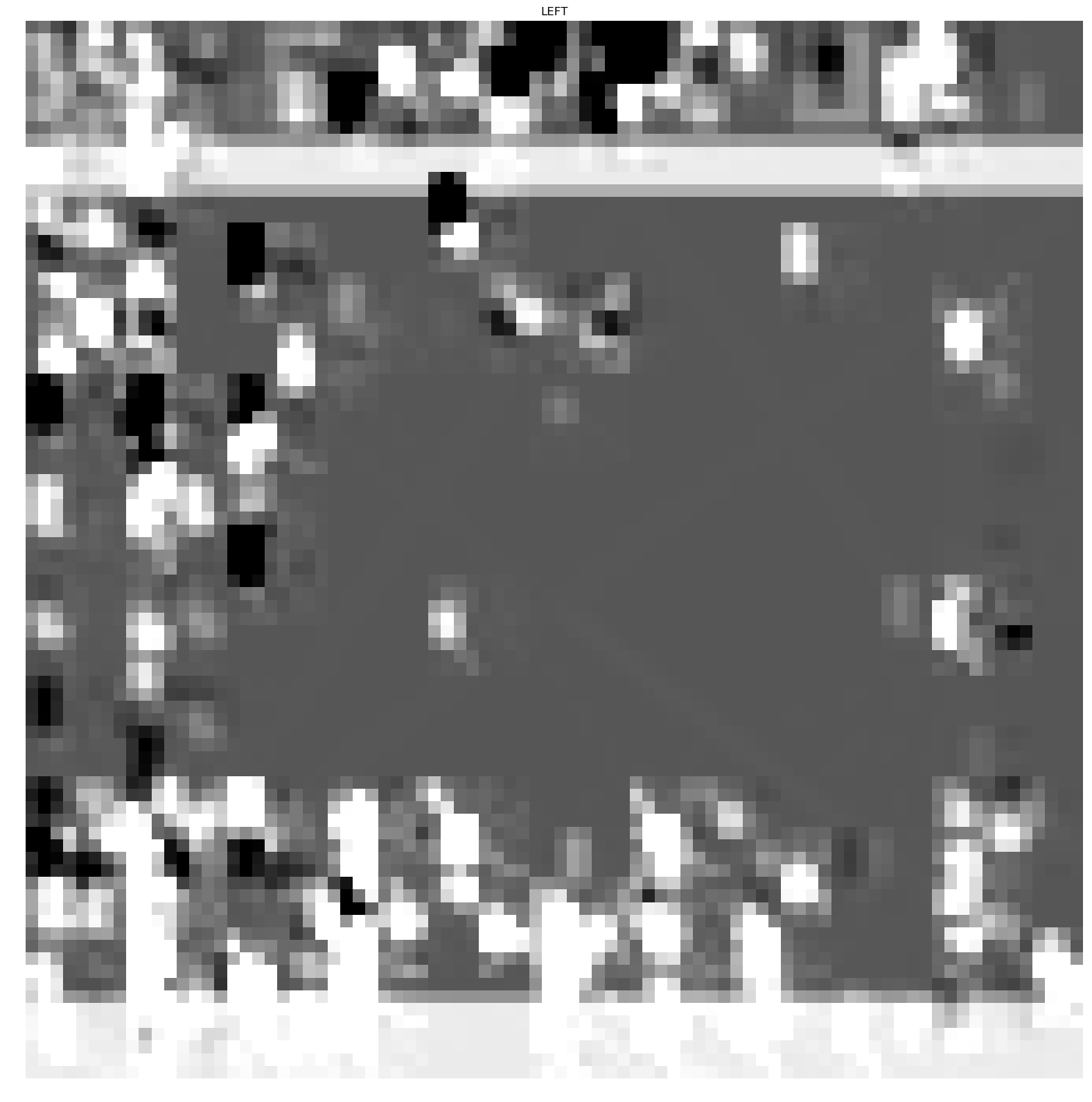
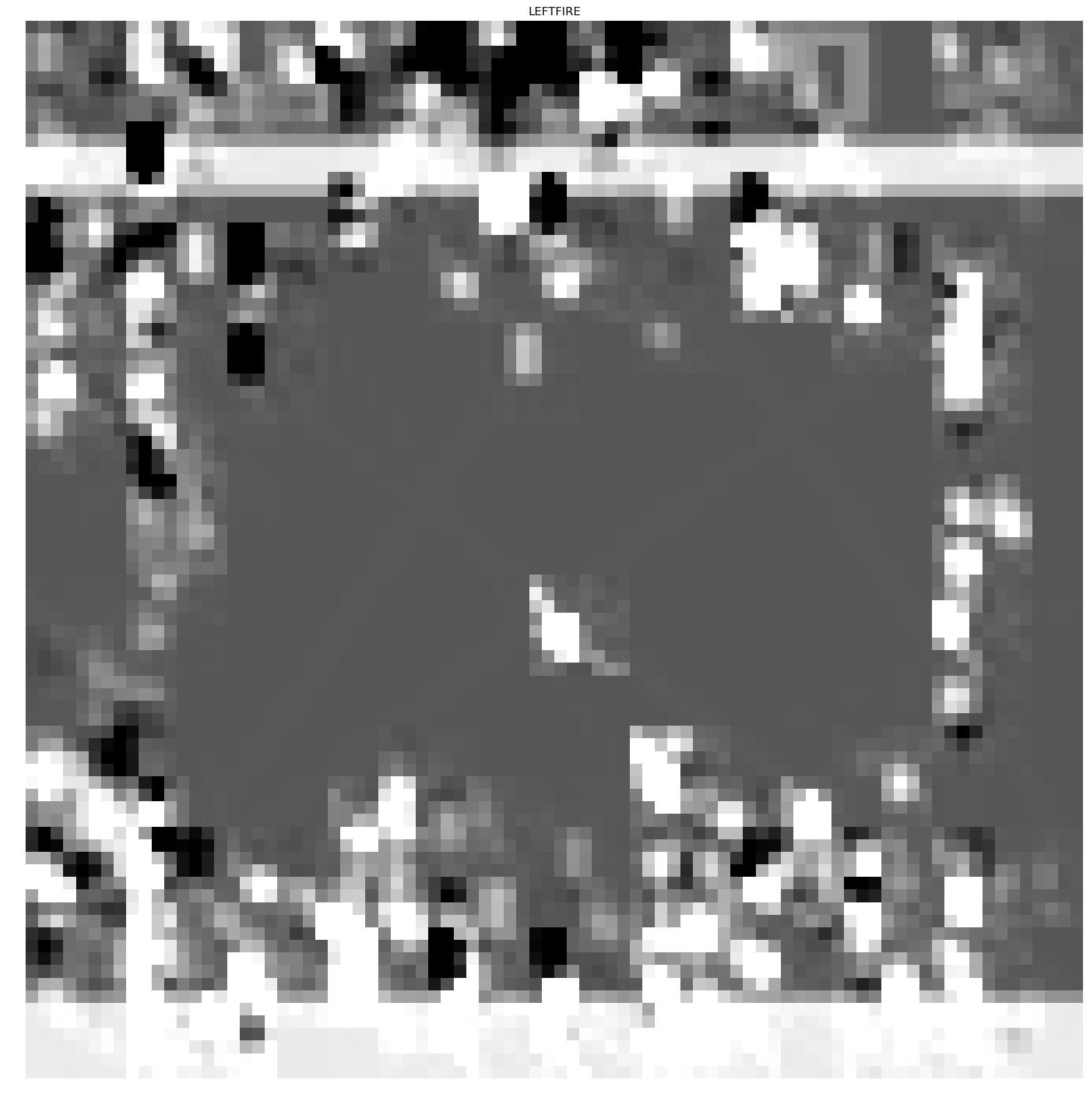
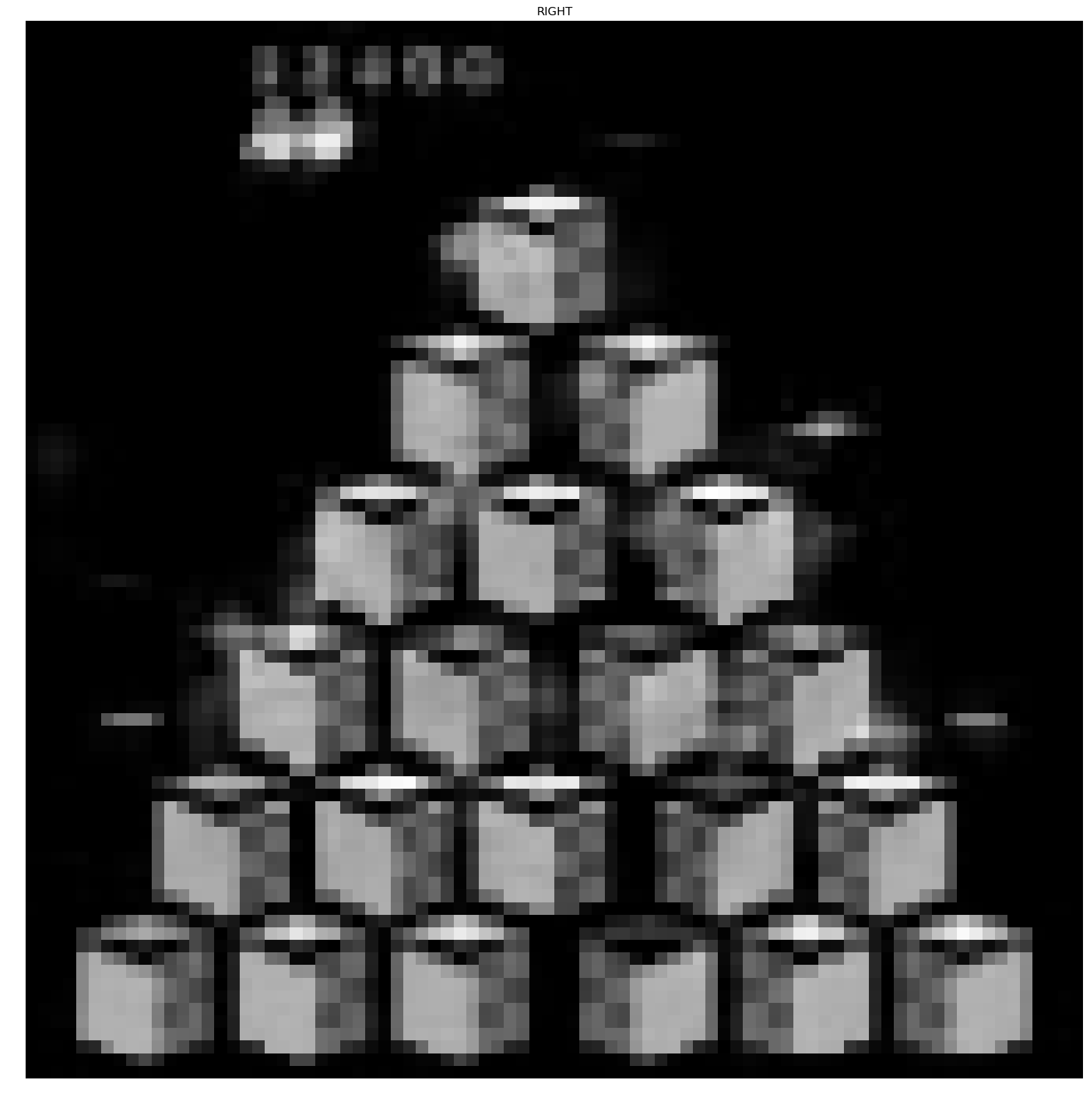
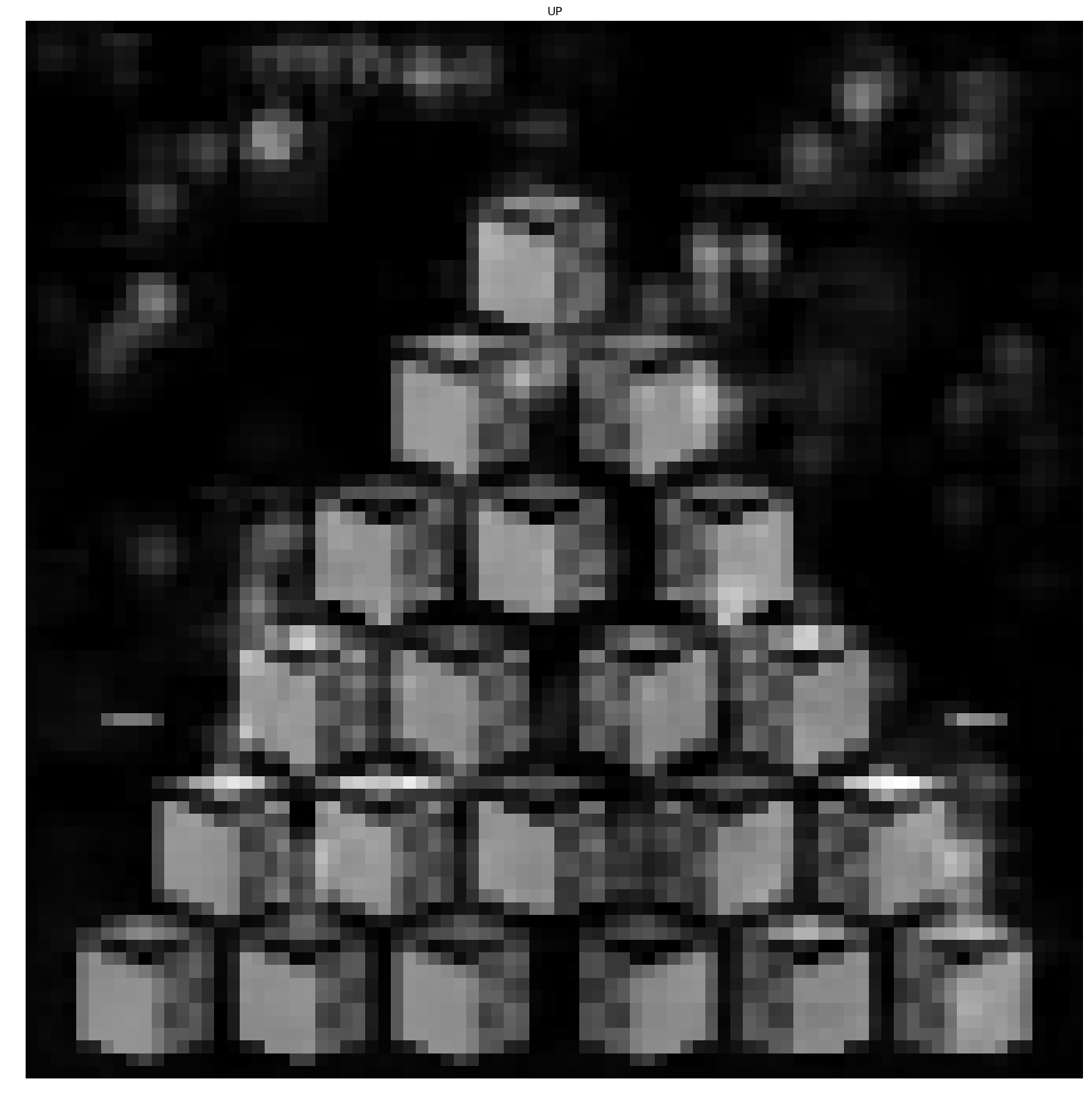
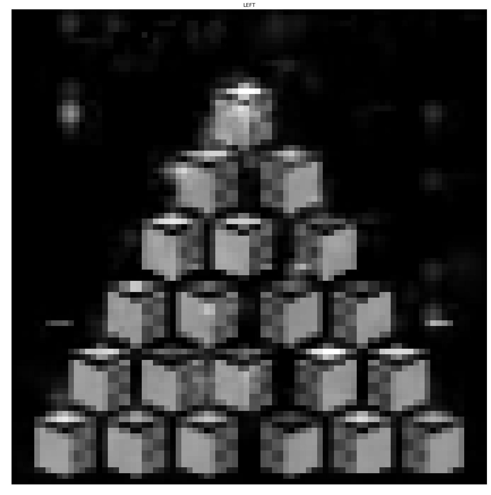
In Figure 16, we show some more examples for MsPacman where the agent does not learn to clear a pellet or goes around repeating action sequences performed during training. Note that Open AI gym environment does not provide access to the state-space and the required out-of-sample state needs to be generated via human gameplay. Figures 18, 18 present an interesting adversarial example created by taking the pixel-wise maximum over real training states. Even though this state is not a valid state, we see that in the attention-maps, all of the four selected actions are strongly highlighted. In fact, by computing the saliency maps with respect to each of these actions, we can almost get back the same regions that are highlighted in Figure 18. This suggests that the key embeddings seem to independently capture specific regions of the board where Pacman is present without modeling any high level dependencies among objects.
