Indefinite Integration Operator Identities and their Polynomial Approximations

Abstract

The integration operators (*) $({\mathcal{J}}^{+}\,g)(x)=\int_{a}^{x}g(t)\,dt$ , $({\mathcal{J}}^{-}\,g)(x)=\int_{x}^{b}g(t)\,dt$ defined on an interval $(a,b)\subseteq{\mathbf{R}}$ yield new identities for indefinite convolutions, control theory, Laplace and Fourier transform inversion, solution of differential equations, and solution of the classical Wiener–Hopf integral equations. These identities are are expressed in terms of ${\mathcal{J}}^{\mp}$  and they are thus esoteric. However the integrals (*) can be approximated in many ways, yielding novel and very accurate methods of approximating all of the above listed relations. Several examples are presented, using Legendre polynomial as approximations, and references are given for approximation of some of the operations using Sinc methods. These examples illustrate for a class of sampled statistical models, the possibility of reconstructing models much more efficiently than by the usual slow Monte–Carlo $({\mathcal{O}}(N^{-1/2})$ rate. Our examples illustrate that we need only sample at $5$ points to get a representation of a model that is uniformly accurate to nearly $3$ significant figure accuracy.

Keywords: Indefinite integration, indefinite convolution, Fourier transform inversion, Laplace transform inversion, Wiener-Hopf, differential equations, approximations
AMS Subject Classification: 47A57, 47A58, 65D05, 65L05, 65M70, 65R10, 65T99, 93C05

1 Introduction and Summary

This paper presents some symbolic–like approximations gotten from identities – some previously known, and some new – of indefinite integration operators. These operators are defined for an interval $(a,b)\subseteq{\mathbf{R}}$ by the equations

$$\begin{array}[]{rcl}({\mathcal{J}}^{+}\,g)(x)&=&\displaystyle\int_{a}^{x}g(t)\,dt\\ &&\\ ({\mathcal{J}}^{-}\,g)(x)&=&\displaystyle\int_{x}^{b}g(t)\,dt\,.\end{array}$$ (1.1)

Here $g$ is a function defined on $(a,b)$ , and we assume, of course, that the integrals exist for all $x\in(a,b)$ . Combined with convolution [Sp], Laplace and Fourier transform inversion, these operators enable many new expressions for one–dimensional models, of: control theory, for Laplace and Fourier transform inversion, for solving ODE [DS] and PDE [Fc, Sc], and for solving Wiener–Hopf integral equations. These operations can be readily combined to get multidimensional approximations. And while these formulas, expressed in terms of ${\mathcal{J}}^{\mp}$ are esoteric, and seemingly devoid of any practical value, when replaced with certain types of approximation in terms of interpolation on $(a,b)$ , yield novel, accurate and efficient methods of approximation. The mode or operations of this paper also enables defining models accurately in terms of statistical samples, but instead of sampling over the whole interval, it suffices to sample at just a small number of points on the interval . Thus, with respect to our illustrative one dimensional examples in this paper, for which we sample at just 5 points, we can recover the model using $5^{2}=25$ points, in $2$ dimensions, $5^{3}=125$ points in $3$ dimensions, etc.

A formula for the approximation of the indefinite integral was first published in [Si], albeit without proof. The first proof was published by Kearfott [K] and later, two proofs were published by Haber [Ha]. The author later presented a proof of this result in §4.5 of [Sp]. These approximation formulas were applied in [Fc] and [Sc] to solve partial differential equations (PDE), via use of explicit Laplace transforms derived by the author of the Poisson, the heat and the wave equation Green’s functions in one and in more than one dimension. In [STB], the Laplace transform of the heat equation Green’s function in ${\mathbf{R}}^{3}\times(0,\infty)$ was used to obtain a numerical solution of the Navier–Stokes equations, and in [SKB] the Fourier transform of this same Green’s function was used to obtain a numerical solution of the Schrödinger equation in ${\mathbf{R}}^{3}\times(0,T)$. More recently, in [Srh], the author constructed a proof of the Riemann hypothesis by use of the operators ${\mathcal{J}}^{\mp}$ .

In §2 we present the operators ${\mathcal{J}}^{\mp}$ , along with some of their properties, as well as methods of approximating the operations of these operators. In addition, we present identities for optimal control, Laplace transform inversion, and the solution of Wiener–Hopf integral equations, as well as identities that are based on Fourier transforms for optimal control, for Fourier transform inversion, for the solution of ordinary differential equations, and for the solution of Wiener–Hopf integral equations. Some of these formulas – the ones involving Laplace transforms – were previously known [Sp], whereas those related to Fourier transforms are new. We have also omitted the relation of these operators with solution of PDE, since this aspect was covered extensively in [Sc].

In §3 we illustrate explicit the application of the esoteric formulas developed in §2; the replacement of ${\mathcal{J}}^{\mp}$ of the formulas of §2 with explicitly defined matrices $A^{\mp}$ transform these esoteric identities into accurate and efficient novel methods of approximation. The matrices that have been used to date are based on either Sinc or Fourier polynomials. Sinc methods have previously been used to define these matrices (see e.g., [Sc], [STB], [SKB], [SA] and [SG]); we have restricted our examples to using Legendre polynomials to define and use the matrices $A^{\mp}$ , since the use of other methods of approximation is similar.

An important property of the matrices $A^{\mp}$ which enables the functions of the matrices $F(A^{\mp})$ which are gotten by replacement of ${\mathcal{J}}^{\mp}$ with $A^{\mp}$ in the operator expression $F({\mathcal{J}}^{\mp})$ to be well defined is that the eigenvalues of $A^{\mp}$ are located on the right half of the complex plane ${\mathbf{C}}$ . This was a 20–year conjecture for Sinc methods; a proof of this conjecture was first achieved by Han & Xu [HX]. A proof was obtained by Gautschi & Hairer [GH] for Legendre polynomials, but a proof for the case of polynomials that are orthogonal over an interval with respect to a positive weight function is still an open problem; this author author offers $300 for the first proof or disproof, that the real parts of all of the eigenvalues of the corresponding integration matrices defined in Definition 3.1 of this paper have positive real parts.

2 The Hilbert space and the operators

It is most convenient to work with operators in the setting of a Hilbert space. Let $(a,b)\subseteq{\mathbf{R}}$ . Our Hilbert space is just the well–known space ${\mathbf{H}}={\mathbf{L}}^{2}(0,b)$ , with $b\in{\mathbf{R}}^{+}$ .

2.1 The operators ${\mathcal{J}}$

Let the operators ${\mathcal{J}}^{\mp}$ be defined for ${\mathbf{H}}$ . The inverses of these operators have the property: if $G={\mathcal{J}}^{\mp}\,g$ , then $g=\left({\mathcal{J}}^{\mp}\right)^{-1}\,G$ , i.e., $g(t)=\mp\,\frac{d}{dt}\,G(t)$ , whenever the derivatives exist.

2.2 Numerical ranges

We mention here some properties of numerical ranges for the operators ${\mathcal{J}}^{\mp}$ .

Definition 2.1.

Let ${\mathbf{H}}$ be defined as above, and let the operators ${\mathcal{J}}^{\mp}$ be defined as in (1.1). The numerical range ${\mathbf{W}}$ of ${\mathcal{J}}^{\mp}$ in ${\mathbf{H}}$ is defined as

$${\mathbf{W}}=\{({\mathcal{J}}^{\mp}\,f,f):f\in{\mathbf{H}}\,,\ \ {\rm with}\ \ \ \|f\|=(f,f)^{1/2}=1\}\,.$$ (2.1)

“Numerical range” is synonymous with “field of values” with the latter being used more often for matrices. The closure of the numerical range of ${\mathcal{J}}^{\mp}$ contains the spectrum of ${\mathcal{J}}^{\mp}$ . Other properties of the numerical range can be found, for example, in [GR] and in [Sh] .

Theorem 2.2.

Let ${\mathcal{J}}^{\mp}$ be defined as in Definition 2.1. Then:

(i.) The numerical ranges of ${\mathcal{J}}^{\mp}$ are contained in the closed right half plane, $\{z\in{\mathbf{C}}:\Re z\geq 0\}$ .

(ii) The real part of the numerical range of $\mp\left({\mathcal{J}}^{\mp}\right)^{-1}$ is $(1/2)(|f(b)|^{2}-|f(a)|^{2})$ .

Proof.  Part(i.): We give a proof of the (i.)–part of this theorem only for the case of ${\mathcal{J}}^{+}$ , inasmuch as the proof for ${\mathcal{J}}^{-}$ is similar.

Let $g\in{\mathbf{H}}$ denote a complex valued function. Then

$$\begin{array}[]{rcl}\Re\left({\mathcal{J}}^{+}\,g,g\right)&=&\displaystyle\Re\int_{a}^{b}\overline{\int_{a}^{x}g(t)\,dt}\,g(x)\,dx\,,\\ &&\\ &=&\displaystyle\frac{1}{2}\,\left|\int_{a}^{b}g(x)\,dx\right|^{2}\geq 0\,,\end{array}$$ (2.2)

so that the inner product $({\mathcal{J}}^{+}\,g,g)$ is contained in the closed right half plane.

Part (ii.) We also omit the straight–forward proof of this part of the theorem.

$\blacksquare$

Theorem 2.3.

Let $(0,b)\subset{\mathbf{R}}$ be a finite interval, let the Hilbert space ${\mathbf{H}}$ be ${\mathbf{L}}^{2}(0,b)$ . Then

$$\|{\mathcal{J}}^{+}\|\leq\frac{b}{\sqrt{2}}\,.$$ (2.3)

Proof.  Let $g\in{\mathbf{L}}^{2}(a,b)$ . Then we have

$$\begin{array}[]{rcl}\|{\mathcal{J}}^{+}\,g\|^{2}&=&\displaystyle\int_{0}^{b}\overline{\int_{0}^{x}g(t)\,dt}\,\int_{0}^{x}g(\tau)\,d\tau\,dx\\ &&\\ &\leq&\displaystyle\int_{0}^{b}\,\left(\int_{a}^{x}1\,|g(t)|\,dt\right)^{2}dx\\ &&\\ &\leq&\displaystyle\int_{0}^{b}x\,dx\,\int_{0}^{x}|g(t)|^{2}\,dt\\ &&\\ &=&\displaystyle\frac{b^{2}}{2}\,\|g\|^{2}\,,\end{array}$$ (2.4)

which yields (2.3).

$\blacksquare$

2.3 Indefinite Convolution via Fourier Transforms

We now take $(0,b)={\mathbf{R}}^{+}$ , where ${\mathbf{R}}^{+}$ denotes the interval $(0,\infty)$ , we take $f^{\mp}\in{\mathbf{H}}={\mathbf{L}}^{2}({\mathbf{R}}^{+})$ , and we assume the usual Fourier and inverse Fourier transforms defined by

$$\begin{array}[]{rcl}\widehat{f^{\mp}}(y)&=&\displaystyle\int_{{\mathbf{R}}^{+}}f^{\mp}(x)\,e^{\mp\,i\,x\,y}\,dx\\ &&\\ f^{\mp}(x)&=&\displaystyle\frac{1}{2\,\pi}\int_{\mathbf{R}}e^{\mp\,i\,x\,y}\,\widehat{f^{\mp}}(y)\,dy\,.\end{array}$$ (2.5)

Theorem 2.4.

If $F^{\mp}:=\widehat{f^{\mp}}$ is the Fourier transform of $f^{\mp}\in{\mathbf{H}}$ , if ${\mathcal{J}}^{\mp}$ is supported on ${\mathbf{R}}^{+}$ , if $(F^{\mp})^{\prime}$ exists on $[0,\infty]$ , and if $f^{\mp}$ is real–valued on ${\mathbf{R}}^{+}$ , then

$$\begin{array}[]{rcl}(\mp i/{\mathcal{J}}^{\mp}\,F^{\mp},F^{\mp})&=&\pm\,\displaystyle\pi\,\int_{{\mathbf{R}}^{+}}y\,|f^{\mp}(y)|^{2}+\frac{i}{2}\,\left(\int_{{\mathbf{R}}^{+}}f^{\mp}(y)\,dy\right)^{2}\,,\\ &&\\ (\mp i/{\mathcal{J}}^{\mp}\,F^{\pm},F^{\pm})&=&\mp\displaystyle\pi\,\int_{{\mathbf{R}}^{+}}y\,|f^{\mp}(y)|^{2}-\frac{i}{2}\,\left(\int_{{\mathbf{R}}^{+}}f^{\mp}(y)\,dy\right)^{2}\,.\end{array}$$ (2.6)

Proof.  We shall prove this lemma only for the case of ${\mathcal{J}}^{+}$ acting on $F^{+}$ , since the proofs for the other cases are similar.

By taking $F^{+}=u+i\,v$ where $F^{+}$ is the Fourier transform of $f^{+}\in{\mathbf{H}}$ taken over ${\mathbf{R}}^{+}$ , we have,

$$\begin{array}[]{rcl}\Im\left(i/{\mathcal{J}}^{+}\,F^{+}\,,F^{+}\right)&=&\displaystyle\Im\int_{{\mathbf{R}}^{+}}\overline{i\,(F^{+})^{\prime}}(x)\,F^{+}(x)\,dx\\ &&\\ &=&\displaystyle-\,\frac{1}{2}\,\left.(u^{2}(x)+v^{2}(x))\right|_{0}^{\infty}\,,\\ &&\\ &=&\displaystyle\frac{1}{2}\,|F^{+}(0)|^{2}\\ &&\\ &=&\displaystyle\frac{1}{2}\,\left(\int_{{\mathbf{R}}^{+}}f^{+}(y)\,dy\right)^{2}\,.\end{array}$$ (2.7)

Note, the term in the last line cannot be negative. If the functions $f\in{\mathbf{H}}$ belongs to ${\mathbf{L}}^{1}({\mathbf{R}})$ , then the term $u^{2}(\infty)+v^{2}(\infty)=0$ , since then $|F(x)|^{2}\to 0$ as $x\to\infty$ , by the Riemann–Lebesgue lemma.

Next, for the real part:

$$\begin{array}[]{l}\Re(i/{\mathcal{J}}^{+}\,F^{+},F^{+})=\\ \\ \displaystyle\Re\,-i\,\int_{{\mathbf{R}}^{+}}\overline{\frac{{\partial}}{{\partial}x}\,\int_{{\mathbf{R}}^{+}}e^{i\,x\,y}\,f^{+}(y)\,dy}\,\int_{{\mathbf{R}}^{+}}e^{i\,x\,\eta}\,f^{+}(\eta)\,d\eta\,dx\\ \\ =\displaystyle\Re-i\lim_{{\varepsilon}\to 0^{+}}\int_{{\mathbf{R}}^{+}}-i\,y\,\overline{f^{+}(y)}\,\int_{{\mathbf{R}}^{+}}f^{+}(\eta)\,\int_{{\mathbf{R}}^{+}}e^{-\,x({\varepsilon}+i\,(y-\eta))}\,dx\,d\eta\,dy\\ \\ =\displaystyle\int_{{\mathbf{R}}^{+}}-\,\int_{{\mathbf{R}}^{+}}y\,\overline{f^{+}(y)}\,\lim_{{\varepsilon}\to 0}\int\frac{f^{+}(\eta)\,\varepsilon}{(x-\eta)^{2}+{\varepsilon}^{2}}\,d\eta\,dy\\ \\ =\displaystyle-\,\pi\,\int_{{\mathbf{R}}^{+}}y\,|f(y)|^{2}\,dy\,.\end{array}$$ (2.8)

The interchange of the order of integration in (2.8) is permitted since both functions $f(y)$ and $y\,f(y)$ belong to ${\bf L}^{1}({\mathbf{R}}^{+})$ .

This completes the proof of Theorem 2.4 .

$\blacksquare$

2.4 Optimal Control

Our model indefinite integrals for $x\in(0,b)\subseteq(0,\infty)$ corresponding to given functions $f^{\mp}$ and $g$ take the form

$$\begin{array}[]{rcl}q^{+}(x)&=&\displaystyle\int_{0}^{x}f^{+}(x-t)\,g(t)\,dt,\\ &&\\ q^{-}(x)&=&\displaystyle\int_{x}^{b}f^{-}(x-t)\,g(t)\,dt.\end{array}$$ (2.9)

Given one or both functions $\widehat{f^{\mp}}$ in (2.5), we shall obtain a formula for determining $q^{\mp}$ on $(0,b)$ , under the assumption that the indefinite integration operators ${\mathcal{J}}^{\mp}$ are supported on $(0,b)$ .

Novel explicit evaluations of the integrals (2.9) were first obtained in [Sp], §4.6, by use of Laplace transforms. Indeed, many new results were obtained using those formulas, including novel explicit formulas for Laplace transform inversions, novel explicit formulas for evaluating Hilbert transforms (discovered independently by Yamamoto [Y] and Stenger [Sc], §1.5.12), and novel formulas for solving partial differential and convolution type integral equations [Sc]. Included with each of these formulas are very efficient and accurate methods of approximation – most of which are given in [Sc]; these usually are orders of magnitude more efficient than the current popular methods of solving such equations.

We shall now derive similar one dimensional novel convolution formulas based on Fourier transforms.

Theorem 2.5.

Let ${\mathcal{J}}^{\mp}$ be defined as above, and have support on $(0,b)\subseteq{\mathbf{R}}^{+}$ , let the functions $f^{\mp}$ of equation (2.6) belong to ${\mathbf{H}}$ . Let $q^{\mp}$ be defined as in (2.6). Then

$$q^{\mp}=\widehat{f^{\mp}}\left(\mp i\,/{\mathcal{J}}^{\mp}\right)\,g\,.$$ (2.10)

Proof.  The proof resembles that given in §4.6 of [Sp] and §1.5.9 of [Sc] for the case of Laplace transforms. We consider only the case of $f^{+}$ , since the proof for the case of $f^{-}$ is similar. The proof makes use of the following:

• $f^{+}$ has compact support $[0,b]$ , – inasmuch extension to $(0,\beta)$ , or to an infinite interval can be carried out via the usual well–known procedure of analysis, and moreover, our assumptions are consistent with this possibility;

• By Theorem 2.4, the spectrum of $i/{\mathcal{J}}^{+}$ lies in the closed second quadrant of the complex plane, ${\mathbf{C}}$ .

• As can be shown via an easy to prove inequality – see [Sp], §4.6 – namely, that $\left\|{\mathcal{J}}^{\mp}\right\|_{p}\leq\alpha$ for all $p\in[1,\infty]$ , where $(0\,,\alpha)\subset{\mathbf{R}}^{+}$ is the support of ${\mathcal{J}}^{\mp}$ ;

• By inspection of (2.6), $\widehat{f^{+}}$ is analytic in the upper half of the complex plane, and $\widehat{f^{-}}$ is analytic in the lower half; and

• The well–known formulas (2.6), as well as

  $$\begin{array}[]{rcl}\displaystyle\left(\left({\mathcal{J}}^{+}\right)^{n}\,g\right)(x)&=&\displaystyle\int_{0}^{x}\frac{(x-t)^{n-1}}{(n-1)\,!}\,g(t)\,dt\,,\ \ \ n=1\,,2\,,\ldots\,,\\ \\ \widehat{f^{\mp}}(z)&=&\displaystyle\mp\frac{1}{2\,\pi\,i}\int_{\mathbf{R}}\frac{\widehat{f^{\mp}}(t)}{t-z}dt\,,\ \ \ \mp\,\Im z>0\,.\end{array}$$ (2.11)

Hence, applying the above points, for $x\in(0,b)$ , and with $I$ denoting the identity operator, we get

$$\begin{array}[]{rcl}q^{+}(x)&=&\displaystyle\int_{0}^{x}f^{+}(x-\xi)\,g(\xi)\,d\xi\\ &&\\ &=&\displaystyle\int_{0}^{x}\,\left(\frac{1}{2\,\pi}\,\int_{\mathbf{R}}\widehat{f^{+}}(t)\,e^{-\,i\,t\,(x-\xi)}\,dt\,\right)\,g(\xi)\,d\xi\\ &&\\ &=&\displaystyle\frac{1}{2\,\pi}\,\int_{\mathbf{R}}\left(\int_{0}^{x}\,\sum_{n=0}^{\infty}\frac{(-i\,t\,(x-\xi))^{n}}{n\,!}\,g(\xi)\,d\xi\right)\,\widehat{f^{+}}(t)\,dt\\ &&\\ &=&\displaystyle\left(\frac{1}{2\,\pi}\,\int_{\mathbf{R}}{\mathcal{J}}^{+}\,\sum_{n=0}^{\infty}\left(-\,i\,t\,{\mathcal{J}}^{+}\right)^{n}\,\widehat{f^{+}}(t)\,dt\,g\right)(x)\\ &&\\ &=&\displaystyle\left(\left(\frac{1}{2\,\pi\,i}\int_{\mathbf{R}}{\mathcal{J}}^{+}/\left(1+i\,t\,{\mathcal{J}}^{+}\right)\,\widehat{f^{+}}(t)\,dt\right)\,g\,\right)(x)\\ &&\\ &=&\displaystyle\lim_{\delta\to 0^{+}}\left(\frac{1}{2\,\pi\,i}\,\int_{\mathbf{R}}\widehat{f^{+}}(t)/\left(t\,I-i/\left({\mathcal{J}}^{+}+\delta\,I\right)\right)\,dt\,g\right)(x)\\ &&\\ &=&\displaystyle\lim_{\delta\to 0^{+}}\left(\widehat{f^{+}}\left(i/\left({\mathcal{J}}^{+}+\delta\,I\right)\right)\,g\right)(x)=\left(\widehat{f^{+}}\left(i/{\mathcal{J}}^{+}\right)\,g\right)(x)\,,\end{array}$$ (2.12)

Similarly, $q^{-}(x)=\left(\widehat{f^{-}}\left(-i/{\mathcal{J}}^{-}\right)\,g\right)(x)$ .

$\blacksquare$

The above identities (2.7) are esoteric. They do, however readily enable applications. See §4.6 of [Sp], or [Sc].

2.5 Fourier transform inversion.

We describe here an explicit novel formula for the inversion of Fourier integrals, namely for the determination of $f^{\mp}$ given $\widehat{f^{\mp}}$, where $\widehat{f^{\mp}}$ are the Fourier transforms of $f^{\mp}$ as defined in (2.7).

Theorem 2.6.

Let ${\mathbf{R}}^{+}$ denote the interval $(0,\infty)$ , and let us assume that we are given one or both of the functions $\widehat{f^{\mp}}$ where,

$$\widehat{f^{\mp}}(x)=\displaystyle\int_{{\mathbf{R}}^{+}}\,e^{\mp\,i\,x\,y}\,f^{\mp}(y)\,dy.$$ (2.13)

Let the operators ${\mathcal{J}}^{\mp}$ have support on $(0,b)\subseteq{\mathbf{R}}^{+}$ . Then, for given $\widehat{f^{\mp}}$ on $(0,b)$ ,

$$f^{\mp}=\displaystyle\left(1/{\mathcal{J}}^{\mp}\right)\,\widehat{f^{\mp}}\left(\mp\,i/{\mathcal{J}}^{\mp}\right)\,1\,,$$ (2.14)

where the “$1$” on the right hand side of (2.14) denotes the function that is identically $1$ at all points of $(0,b)$ .

Proof.  We shall only prove this theorem for the case of $f^{+}$ , inasmuch as the proof for the case of $f^{-}$ is similar.

Let us first recall, by assumption, that $f^{\mp}$ is differentiable. Then

$$\begin{array}[]{rcl}f^{+}(x)-f^{+}(0)&=&\displaystyle\int_{0}^{x}\left(f^{+}(y)\right)^{\prime}\,dy\\ &&\\ &=&\displaystyle\int_{0}^{x}\left(f^{+}\right)^{\prime}(x-y)\,dy\\ &&\\ &=&\displaystyle\int_{0}^{x}\left(f^{+}\right)^{\prime}(x-y)\,1\,dy\,.\end{array}$$ (2.15)

This equation is now in the form of the equation for $q^{+}$ in (2.9), except that $q^{+}$ in (2.9) is here replaced with the derivative $\left(f^{+}\right)^{\prime}$ , and $g$ with the the function that has value $1$ on $(0,b)$ . Hence, using the Fourier transform $-i\,x\,\widehat{f^{+}}(x)+f(0)$ of $\left(f^{+}\right)^{\prime}$ and substituting into (2.15)  we get the equation (2.10) for the case of $f^{+}$ .

$\blacksquare$

The identities (2.10) and (2.15), while esoteric, can nevertheless yield applicable approximations in suitable analytic function settings, as they did for the case of Laplace transforms in [Sp] and in [Sc].

Remark 2.7.

If we substitute $y=\mp\,i\,\eta$ in (4.1), we are then back to the Laplace transform cases already covered extensively, starting with [Sp], §4.5–4.6, and then followed up with all of the text, [Sc] . These sources cover the operator results of this section, elucidating them to approximation via use of Cauchy sequences of analytic functions based on Sinc methods of approximation.

We should add, that the two main theorems of this section have applications not only to approximation via Sinc methods, but also, to any other method of approximation, including methods that use orthogonal polynomials.

3 Connection with interpolatory approximation

The formulas derived in the previous section are esoteric, but they have many applications when connected with interpolatory approximation.

(i.) For the case Legendre polynomials, the $x_{j}$ are the $n$ zeros of the Legendre polynomial $P_{n}(x)$ which are orthogonal on the interval $(a,b)=(-1,1)$ with respect to the weight function $w$ which is identically $1$ on $(-1,1)$ ;

(ii.) For the case of Hermite polynomial interpolation, using the Hermite polynomials $H_{n}(x)$ that are orthogonal over ${\mathbf{R}}$ with respect to the weight function $w$ , with $w(x)=\exp(-x^{2})$, and with $H_{n}(x_{j})=0$ for $j=1\,,\ \ldots\,,\ n$ ; and

(iii.) Other polynomials that are orthogonal with respect to a weight function, such as Jacobi polynomials, Gegenbauer polynomials, etc.

Definition 3.1.

Consider standard Lagrange interpolation at distinct points $x_{j}$ , with $a<x_{1}<x_{2}\ldots x_{n}<b$

$$\begin{array}[]{rcl}f(x)&\approx&\displaystyle\sum_{k=1}^{n}\ell_{k}(x)\,f(x_{k})\,,\\ &&\\ \ell_{k}(x)&=&\displaystyle\prod_{j=1\,,\ \ldots\,,\ n,\ \ j\neq k}\frac{x-x_{j}}{x_{k}-x_{j}}\,,\end{array}$$ (3.1)

we introduce a family of $n\times n$ matrices $A^{\mp}=\left[A_{j,k}^{\mp}\right]$ for which the entries $A_{j,k}^{\mp}$ are defined by

$$\begin{array}[]{rcl}A_{j,k}^{+}&=&\displaystyle\int_{a}^{x_{j}}\ell_{k}(x)\,w(x)\,dx\,,\\ \\ &&\\ A_{j,k}^{-}&=&\displaystyle\int_{x_{j}}^{b}\ell_{k}(x)\,w(x)\,dx\,,\end{array}$$ (3.2)

where $w$ is a weight function that is positive a.e. on $(a,b)$ , such that the moments $\int_{a}^{b}w(x)\,x^{j}\,dx$ exist for every non–negative integer $j$ .

Setting

$$\begin{array}[]{rcl}V\,f&=&(f(x_{1})\,,\ \ldots\,,\ f(x_{n}))^{T}\\ &&\\ L(x)&=&(\ell_{1}(x)\,,\ \ldots\,,\ \ell_{n}(x))\,,\end{array}$$ (3.3)

and defining ${\mathcal{J}}^{\mp}_{n}$ by

$$({\mathcal{J}}^{\mp}_{n}\,w\,f)(x)=L(x)A^{\mp}\,V\,{\bf f}\,,$$ (3.4)

so that if, for $D=\Im\mp z>0$ , and if $\hat{f}$ is analytic in $D$ , then the eigenvalues of $\mp i\,A^{\mp}$ lie in $D$ , so that the matrix $\hat{f}(\mp i\,(A^{\mp})^{-1})$ is then well defined, as also, is the approximation

$$V\,\hat{f}(\mp\,i/{\mathcal{J}}^{\mp})\,g\approx\hat{f}\left(\mp i\,(A^{\mp})^{-1}\right)\,V\,g\,.$$ (3.5)

Remark 3.2.

(i.) The last line of (3.5) can be explicitly evaluated. If for the case of $A^{+}$ (resp., if for the case of $A^{-}$ we have $A^{+}=X\,\Lambda\,X^{-1}$ (resp., $A^{-}=Y\,\Lambda\,Y^{-1}$), where $\Lambda={\rm diag}(\lambda_{1},\ \ldots\,\ \lambda_{n})$ is the diagonal matrix, which is the same for $A^{+}$ and $A^{-}$ , and where $X$ (resp., $Y$) is the corresponding matrix of eigenvectors, then

$$\begin{array}[]{rcl}\widehat{f^{+}}\left(i\,(A^{+})^{-1}\right)\,V\,g=X\,{\rm diag}(i/\lambda_{1},\ \ldots,\ i/\lambda_{n})\,X^{-1}\,V\,g\,,\end{array}$$ (3.6)

and similarly for the term involving $\widehat{f^{-}}\,,A^{-}$ and $Y$ .

(ii.) If for (i.) above, the matrices $A^{\mp}$ are defined for $(-1,1)$ , then for any other interval $(a,b)$ , $A^{\mp}$ needs to be replaced with $C^{\mp}=(b-a)/2$ ; this means that the eigenvalues $\lambda_{j}$ are also to replaced with $(b-a)/2$ , but the matrix of eigenvectors remains unchanged.

Conjecture. We state the following conjecture, for which the author of this paper offers $300 for the first proof or disproof:

All of the eigenvalues of each the $n\times n$ matrices $A^{\mp}$ that are defined as in Definition 3.1 for all polynomials $\{p_{n}\}$ which are orthogonal over $(a,b)$ with respect to the weight function $w$ lie on the open right half of the complex plane.

This conjecture has been shown to be true for Sinc interpolation by Han and Xu [HX]; it has also been shown to be true for Legendre polynomial interpolation by Gautschi and Hairer [GH]. However, the conjecture as stated for Definition 3.1 is still unproved for arbitrary weight functions $w$ that are positive a.e. on $(a,b)$ .

The following result, can also be of use in applications. We select for this theorem the weighted Hilbert space ${\bf H}_{w}$ of all functions $f,\ g,\ \ldots,$ with inner product

$$(f,g)=\displaystyle\int_{-1}^{1}w(x)\,\overline{f(x)}\,g(x)\,dx\,,$$ (3.7)

where $w$ is defined in Definition 3.1. The transformation of this formula to the interval $(a,b)$ via use of the transformation $x=t(y):=(a+b)/2+y\,(b-a)/2$ takes the form

$$(f,g)=(F,G)_{(a,b)}=\displaystyle\int_{a}^{b}W(y)\,\overline{F(y)}\,G(y)\,\frac{b-a}{2}\,dy\,,$$ (3.8)

where $W(y)=w(t(y))$ , $F(y)=f(t(y))$, and $G(y)=g(t(y))$ . The proof of the following result is straight–forward, and we omit it.

Theorem 3.3.

Let the operators ${\mathcal{J}}^{\mp}$ be defined as in Definition 2.2. If $f\in{\mathbf{H}}_{w}$ , then

$$\begin{array}[]{l}\displaystyle\left|\int_{a}^{b}W(y)\,\overline{F(y)}\,\int_{a}^{y}W(t)\,F(t)\,dt\,dy\right|=\displaystyle\frac{(b-a)^{2}}{2}\,\left|\int_{-1}^{1}\overline{f(\eta)}\,\int_{-1}^{\eta}f(\xi)\,d\xi\,d\eta\right|\,,\\ \\ \leq\displaystyle\frac{(b-a)^{2}}{2}\,\int_{-1}^{1}\frac{d}{dx}\int_{-1}^{x}w(t)\,|f(t)|\,dt\,w(x)\,|f(x)|\,dx\\ \\ \leq\displaystyle\frac{(b-a)^{2}}{2}\left(\int_{-1}^{1}w(x)\,|f(x)|\,dx\right)^{2}\,dx\,.\end{array}$$ (3.9)

4 Applications

We illustrate in this section, several examples that ensue by approximation of the integration operators ${\mathcal{J}}^{\mp}$ . Such approximations were first stated in [Sr], then proved by Kearfott [K], Haber [H] and the author [Sp], §4.5. approximation based on using the operators ${\mathcal{J}}^{\mp}$. The use of these operators for obtaining numerical solutions of differential and integral equations was first discovered by the author in [Sp], and these were combined extensively in [Sc], with formulas for approximating the indefinite integral. The present section illustrates applications by combining indefinite integration with Lagrange polynomial approximation.

4.1 Legendre polynomial approximation of a model

For sake of simplicity, we use only Legendre polynomials as approximations, since applications using other bases are dealt with in exactly the same way. We also use polynomials of degree at most $4$ , in view of the present wide–spread interest in problems arising from using large sets of data values. Under the assumption of analyticity of the reconstruction (see e.g., §2 of [Sc]), we get effective answers to problems whose solutions are smooth, using a very small number of points to construct a solution. That is, the explicit numerical examples of this section are most effective for cases when the model to be approximated is smooth.

It is well known that if a function $f$ is analytic in a simply connected domain $D$ in the complex plane, and if a closed interval $[a,b]$ is in the interior of $D$ , then we can approximate $f$ on $[a,b]$ via a polynomial of degree $n$ for which the error approaches zero at a rate of ${\mathcal{O}}(\exp(-\,c\,n))$ where $c$ is a positive constant. To be more specific, if $(a,b)=(-1,1)$, and if we let $\phi_{j}$ denote the normalized Legendre polynomial of degree $j$ , so that $\int_{-1}^{1}\phi_{j}(x)\,\phi_{k}(x)\,dx=\delta_{j,k}$ where $\delta_{j,k}$ denotes the Kronecker delta, then the numbers $c_{k}=\int_{-1}^{1}f(x)\,\phi(x)dx$ approach zero exponentially, and the approximation

$$f(x)\approx\sum_{k=0}^{n}c_{k}\,\phi_{k}(x)$$ (4.1)

will then be accurate for a relatively small value of $n$ . To this end, we could start with a positive integer $m$ (with $m=5$ in this paper), then, letting $x_{1}\,,\ \ldots\,,\ x_{m}$ denote the distinct zeros of $\phi_{m}$, and letting $w_{1}\,,\ \ldots\,,\ w_{m}$ denote the corresponding Gaussian integration weights, we could evaluate numbers $c_{1}\,,\ \ldots\,,\ c_{n}$ , with the formula

$$c_{k}\approx\displaystyle\sum_{\ell=0}^{m}w_{\ell}\,f(x_{\ell})\,\phi_{j}(x_{\ell})$$ (4.2)

and stop the process, when $c_{k}$ ($k\leq n$) is sufficiently small, since $c_{n}$ is then of the order of the error of approximation.

The above process can also be used when $f$ is approximated via statistical sampling. In this case, it would be necessary to get a good approximation at the above defined zeros $x_{j}$ , and this can be done in many ways, one of which is $\ell^{1}$–averaging.

Note, also, the well known $m$–point Lagrange interpolation formula, which is used extensively in this section, for evaluating the polynomial $P_{m-1}$ which interpolates a function $f$ at the $m$ points $x_{1}\,,\ \ldots\,,\ x_{m}$:

$$\begin{array}[]{rcl}P_{m-1}(x)&=&\displaystyle\sum_{j=1}^{m}\ell_{k}(x)\,f(x_{k})\,,\\ &&\\ \ell_{k}(x)&=&\displaystyle\prod_{j=1\,,j\neq k}^{m}\frac{x-x_{j}}{x_{k}-x_{j}}\,.\end{array}$$ (4.3)

4.2 Reconstruction from statistical data

Statistical models can take on many different forms, see e.g., [X]. Typically, these can take the form of a system of nonlinear equations, a system of ordinary differential equations (ODE) a system of partial differential equations (PDE), or a system of integral equations, all in the possible presence of noise. The variety of such equations means that many different methods are in use for solving such equations. Included among these are Fokker–Planck models [BS], Navier–Stokes equations [STB], Schrödinger equations [SKB] and the methods used in [Sc] for solving partial differential and integral equations. However, for sake of simplicity we shall restrict or presentation to one–dimensional models, with approximation using Legendre polynomials.

4.3 Exact formulas and their approximation

The formulas which we shall describe below will initially be defined in terms of the operators ${\mathcal{J}}^{\mp}$ , and they thus appear esoteric. However, these operations can readily be approximated via use of computable basis functions. We shall only use approximation via Legendre polynomial interpolation of degree 5 in this section, although the programs can easily be altered to work for arbitrary degrees, and with other bases – for example, the text [Sc] mainly uses sinc functions as bases – although methods based on Fourier polynomial bases are given in §1.4.7 and 3.10.2 of [Sc]. Explicit Matlab programs are available for all of the examples of this section.

(i.) Fourier transform inversion. Statistical modeling at times – such as in connection with vision [GW] – involves the Fourier transforms.

We shall use the formula of Theorem 2 (a).

Consider the trivial example for the recovery of $f$ on $(0,4)$ given $F^{+}(y)=\int_{0}^{\infty}f(t)e^{i\,y\,t}dt=1/(1-i\,y)$ . The exact solution is (*) $f(t)=e^{-t}$ . We use formulas (2.14 ) and (4.3), taking a Legendre polynomial of degree $5$, to get a matrix $A^{+}$ of order $5$ which we multiply by $2$ to get $C=2\,A^{+}$, for approximation on $(0,4)$ , twice the length of the interval $(-1,1)$ . By Theorem 2.6 and Equation (3.4), $y$ in the above Fourier transform is replaced with $i/C$ , and also, selecting the new interpolation points $\xi_{j}=2(1+x_{j})$ , we get

$$(f(\xi_{1})\,,\ \ldots\,,\ f(\xi_{n}))^{T}\approx({\bf I}+C)^{-1}\,{\bf 1}\,,$$ (4.4)

where ${\bf I}$ denotes the unit matrix, ${\bf 1}$ is a vector of $n$ ones, and where the matrix $({\bf I}+C)^{-1}$ is non–singular, since all of the eigenvalues of $A^{+}$ have positive real parts.

Initially we just plot the five exact and computed values at $\xi_{j}=1+x_{j}$. The next plots contain the exact solution $e^{-t}$ , along with the computed approximation evaluated with the polynomial which interpolates the 5 computed values at $\xi_{j}$ . These plots are carried out on a $100$–point equi-spaced mesh. Finally, we also plot the fine-mesh error, i.e., the difference between the exact and computed solution at the same 100 points.

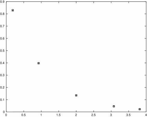
Figure 1: Course mesh plot of exact & computed FT inversion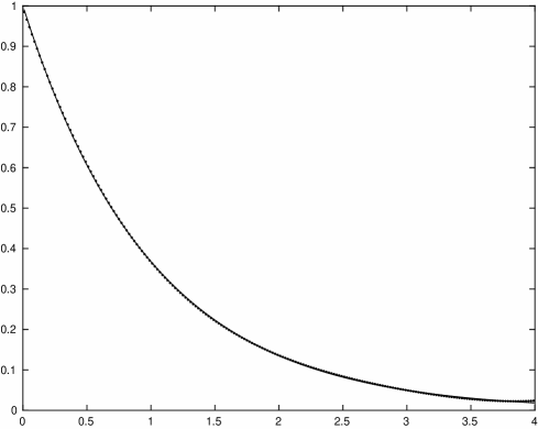

Figure 2: Fine mesh plot of exact & computed FT inversion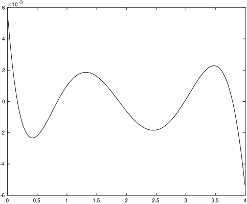

Figure 3: Fine mesh plot of error of FT inversion

(ii.) Laplace transform inversion

The inversion formula for Laplace transform inversion was originally discovered by Stenger in [Sc]. The exact formula used here is only the third known exact formula for inverting the Laplace transform, the other two being due to Post [P] and Bromwich [B]., although we claim that the practical implementation of the Post formula is impossible, while the evaluation of the vertical line formula of Bromwich is both far more difficult and less accurate than our method, which follows.

Consider the case of recovering the following function $f$ on $(0,2)$ given $F$ , where

$$\begin{array}[]{rcl}f(t)&=&\displaystyle\frac{\sin(\pi\,t)}{\pi\,t};\\ &&\\ F(s)&=&\displaystyle\int_{0}^{\infty}f(t)e^{-st}dt=1/2-(1/\pi)\tan^{-1}(s/\pi)\,.\end{array}$$ (4.5)

We again use Lagrange polynomial approximation via interpolation at the zeros of this polynomial of degree $5$ . The length of the interval is $(0,2)$ , which is the same as the length of $(-1,1)$ , for which the matrix $A^{+}$ is defined. The new points of interpolation are on the interval $(0,2)$ which shifts them by $1$ from the original interval $(-1,1)$ for Legendre polynomials, so that the new points of interpolation are $\xi(j)=1+x(j)$ . The exact inversion formula is $f=1/{\mathcal{J}}^{+}\,F(1/{\mathcal{J}}^{+})\,1$ , with $F$ given on the right hand side of (4.5). Hence replacing ${\mathcal{J}}^{+}$ with $A^{+}$ , we get the following exact and approximate solutions:

$$\begin{array}[]{l}f(\xi_{j})=\displaystyle\frac{\sin(\pi\,\xi_{j})}{\pi\,\xi_{j}}\,,\ \ \ j=1\,,\ \ldots\,,\ n\,,\\ \\ (f(\xi_{1})\,,\ldots\,,\ f(\xi_{n}))^{T}\approx(A^{+})^{-1}\,F((A^{+})^{-1})\,{\bf 1}\,,\end{array}$$ (4.6)

where ${\bf 1}$ denotes a column vector of n ones. In this case we need the eigenvalue representation $A^{+}=X\,\Lambda\,X^{-1}$ to evaluate last equation of (4.6). We get

$$(f(\xi_{1})\,,\ \ldots\,,\ f(\xi_{n}))^{T}\approx X\,\Lambda^{-1}\,F(\Lambda^{-1})\,X^{-1}\,{\bf 1}\,.$$ (4.7)

We next plot in fine mesh solution, which is obtained by evaluating the degree $4$ polynomial interpolation of the computed solution at 100 equi–spaced points on $(0,4)$ . Finally, we also plot the fine-mesh error at the same 100 points. The slight error at the end–points is due to the jump singularity of the Fourier transform at the origin.

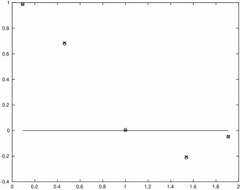
Figure 4: Course mesh plot of exact (-) & computed (.) LT inversion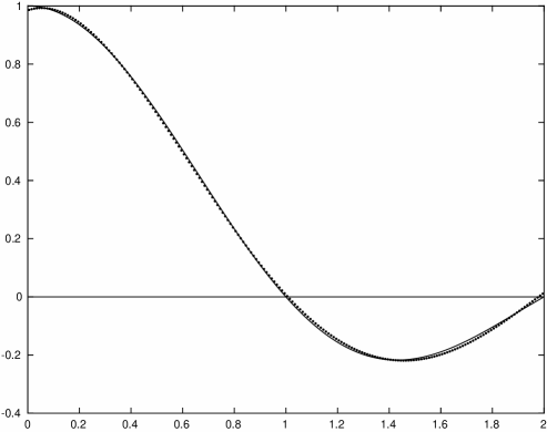

Figure 5: Fine mesh plot of exact (-) & computed (.) LT inversion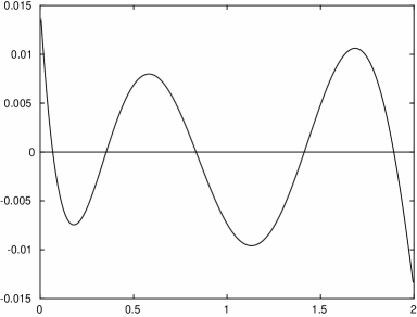

Figure 6: Fine mesh plot of error of LT inversion

(iii.) Optimal control via Fourier transforms

We illustrate here an application of Theorem 2.5.

Such an example may arise in simple design of a control, or in the statistical determination of a feedback control, etc. We wish to evaluate integral

$$p(t)=\int_{t}^{3}f(t-\tau)\,g(\tau)\,d\tau\,,\ \ \ t\in(0,3)\,,$$ (4.8)

using the formula

$$p=\widehat{f}(-i/{\mathcal{J}}^{-})\,g\,,$$ (4.9)

where $\widehat{f}(y)=\int_{-\infty}^{0}f(t)\,e^{i\,y\,t}\,dt=\int_{0}^{\infty}f(-t)\,e^{-i\,y\,t}\,dt$ . Here we shall use the matrix $A^{-}$ defined as in Definition 3.1 above, which must be replaced by $C=(3/2)\,A^{-}$ for use on the interval $(0,3)$ , and in addition, the points of interpolation are $\xi_{j}=(3/2)\,(1+x_{j})$ . Thus the approximation formula is

$$V\,p\approx\widehat{f}(-i\,C^{-1})\,V\,g\,.$$ (4.10)

We consider as an example, the evaluation of the convolution integral

$$\int_{t}^{3}\exp(\alpha\,(t-\tau))\,J_{0}(t-\tau)\,e^{-\,\beta\,\,\tau}\,d\tau\,,\ \ t\in(0,3)\,,$$ (4.11)

where $\alpha$ and $\beta$ are positive. In this case, we have the Fourier transform

$$\widehat{f}(y)=\displaystyle\int_{0}^{\infty}e^{-i\,y\,t-a\,y\,t}\,J_{0}(t)\,dt=\displaystyle\frac{1}{\alpha+i\,y}\,(1+(\alpha+i\,y)^{2})^{-1/2}\,,$$ (4.12)

and upon replacing $y$ with $-i\,C^{-1}$ , we get the approximation

$$\begin{array}[]{rcl}{\bf p}&:=&(p(t_{1})\,,\ \ldots\,,\ p(t_{n}))^{T}\\ &&\\ &\approx&C\,\left((1+\alpha^{2})\,C^{2}+2\,\alpha\,C\,+\,I\right)^{-1/2}\,{\bf g}\\ &&\\ {\bf g}&=&\left(e^{-\,\beta\,t_{1}}\,,\ \ldots\,,\ e^{-\,\beta\,t_{n}}\right)^{T}\,.\end{array}$$ (4.13)

The selection of several values of $\beta$ could be used to model a given output $p$ . The example which follows uses $\beta=0.7$ .

But more directly, since $p$ and $g$ are related by the equation (4.12), we could also determine an accurate control vector ${\mathbf{g}}$ to compute an accurate approximation to the response:

$${\bf g}\approx\left((1+\alpha^{2})\,C^{2}\,+2\,\alpha\,C+I\right)^{-1/2}\,{\bf p}\,.$$ (4.14)

Note here that the matrix multiplying $g$ in (4.13) can be determined explicitly: setting $C=X\,\Lambda\,X^{-1}$ , where $\Lambda={\rm diag}(\lambda_{1}\,,\ \ldots\,,\ \lambda_{n})$ , we have

$$\begin{array}[]{l}D:=X^{-1}\,\left((1+\alpha^{2})\,C^{2}\,+2\,\alpha\,C+I\right)^{1/2}\,X\,;\\ \\ D={\rm diag}(d_{1}\,,\ \ldots\,,\ d_{n});\ \ \ d_{j}=((1+\alpha^{2})\,\lambda_{j}^{2}+2\,\alpha\,\lambda_{j}+1)^{1/2}\,.\end{array}$$ (4.15)

This matrix is non–singular, and we can therefore use it to compute an approximation to the function $g$ in (4.8), in order to achieve a any particular response.

If we again use the same Legendre polynomial of degree 5, we get a polynomial solution, but unfortunately, the exact solution is not explicitly known. To this end, we can use the same equation (4.14), but with a larger value of $n$, to get a more accurate solution; e.g., by taking $n=11$, we get at least $8$ places of accuracy, which can be taken to be the exact answer for our purposes, and which we use to compute the exact answer at $5$ points $\xi_{j}$ . We thus again get $3$ plots as above, i.e., as a course mesh plot of the “exact” and our degree 4 approximation, a fine mesh plot of the “exact” solution and of our degree 4 approximation of this solution, and a fine mesh plot of the difference between these two quantities.

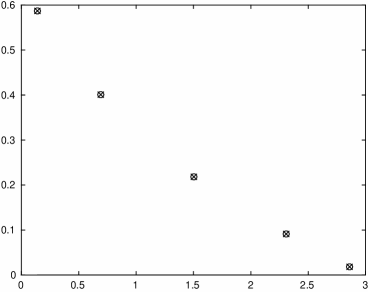
Figure 7: Course mesh plot of exact & computed opt. control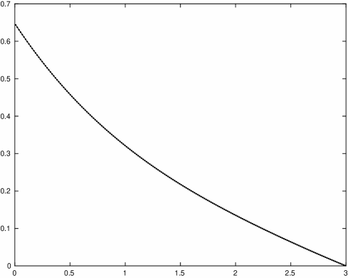

Figure 8: Fine mesh plot of exact & computed opt. control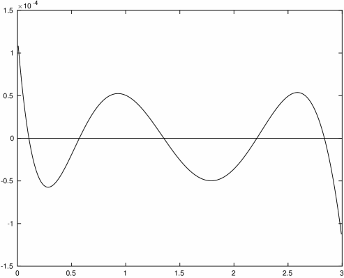

Figure 9: Fine mesh plot of error of opt. control

(iv.) Modeling via ordinary differential equations

Most ODE solvers in use today are one step methods, and as such, their use is restricted because of stability, convergence, stiffness, and accuracy, and moreover, they are restricted to obtaining a solution on a finite interval. Not so with the present method [DS], which extends its usage to polynomials the method of [SA] that was designed for Sinc approximation.

The most common ODE model for constructing methods of approximate solutions of ODE on an interval $(a,b)$ is

$$y^{\prime}=f(x,y)\,,\ \ \ y(a)=y_{a}\ \ \ ({\rm a\ constant})$$ (4.16)

Transforming to an equivalent integral equation, we get

$$y(x)=y_{a}+\displaystyle\int_{a}^{x}f(t,y(t))\,dt\ \ \ {\rm or}\ \ \ y=y_{a}+{\cal J}^{+}\,f(\cdot,y(\cdot)\,1\,.$$ (4.17)

Upon applying the approximation procedure of §3 above, we can immediately convert The IE (4.17) to a system of algebraic equations

$$Y=y_{a}\,{\bf 1}+A^{+}\,{\bf f}\,{\bf 1}\,,$$ (4.18)

where $Y=(y_{1}\,,\ \ldots\,,\ y_{n})^{T}$ , ${\bf I}$ is the unit matrix of size $n$ , $A^{+}$ is as defined in §3.2, and

$${\bf f}:=\left(\begin{array}[]{c}f(x_{1},y_{1})\\ \vdots\\ f(x_{n},y_{n})\end{array}\right)\,.$$ (4.19)

Some notes:

(1) Convergence will always occur for $b-a$ sufficiently small, since it can be shown that the eigenvalues of $\,A$ are bounded by $(b-a)/\sqrt{2}$ .

(2.) Under a test of convergence criteria such as $\|Y^{(m)}-Y^{(m-1)}\|<{\varepsilon}$, the resulting solution will have polynomial degree $n$ accuracy at each of the points $z_{1}\,,\ \ldots\,,\ z_{n}$ where the interpolation is exact . Under mild assumptions on $f$ , we can then achieve similar accuracy at any set of points, e.g., at equi–spaced points.

(3.) Knowing accurate values of both $y$ and $y^{\prime}=f$ at $n$ points, we can get polynomial precision of degree $2\,n-1$ using Hermite interpolation.

Consider the case of recovering the following function $y$ on $(0,1/2)$ , where

$$y\prime=1+y^{2},\ \ \ y(0)=0.$$ (4.20)

The exact solution is $y=\tan(t)$ .

Since the interval is $(0,1/2)$ , the new points of interpolation are $\xi_{j}=(1+x_{j})/2$ , and the corresponding indefinite integration matrix is $C=(1/2)\,A$ .

By applying the above outlined method of approximation, we replace the IE of (31) by the system of algebraic equations

$$Y=X+C\,Y_{2}\,,$$ (4.21)

where $X=(t_{1}\,,\ \ldots\,,\ t_{n})^{T}$ , and $Y_{2}=(y_{1}^{2}\,,\ \ldots\,,\ y_{n}^{2})^{T}$ . The interval $(0,1/2)$ was selected here since, for example, if the matrix $C$ in (4.21) is replaced with $A^{+}$, then Picard iteration does not converge to a solution of (4.20). We could, of course, extend the solution further, by restarting it at $t=1/2$ .

The computed solution and plots are the same as in the previous cases, namely, a course plot of the exact and computed solution at the points $\xi_{j}$ , $j=1\,,\ \ldots\,,\ 5$ , a fine mesh plot at $100$ equi–spaced points of the exact and the computed polynomial solution on the interval $(0,1/2)$ , and a fine mesh plot of the difference between these functions on the same interval.

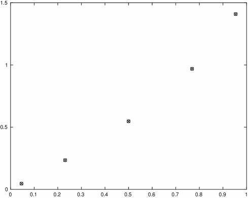
Figure 10: Course mesh plot of exact & computed ODE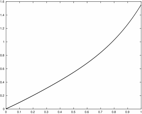

Figure 11: Fine mesh plot of exact & computed ODE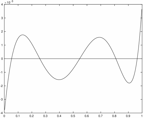

Figure 12: Fine mesh plot of error of ODE

(v.) Modeling via Wiener–Hopf Equations

The classical Wiener–Hopf integral equation with solution $f$ for given $k$ defined on ${\bf R}$ and $g$ defined on $(0,\infty)$ takes the form

$$f(x)-\displaystyle\int_{0}^{\infty}k(x-t)\,f(t)\,dt=g(x)\,,\ \ x\in(0,\infty)\,.$$ (4.22)

Many thousands of papers have been written on the solution of this equation, particularly with reference to the mathematically beautiful factorization procedure originally discovered by Wiener and Hopf in 1931 for solving this equation. Unfortunately, such a factorization cannot be determined for nearly all problems of the type (4.22). A revision to this mathematics among the top 10 mathematics departments occurred from about 1960 until 1970, but none of this pure mathematics activity provided any insight to the solution of (4.22). We illustrate here a method of solving this problem, and while our illustration is almost trivial, in that the exact equation is easier to solve than our approximating equation, our approximating method nevertheless applies to all equations of the the type (4.22). Moreover, the solution we present in what follows is both efficient and accurate.

By splitting the definite convolution integral in (4.22) as an integral from $0$ to $x$ plus an integral from $x$ to $\infty$ , to get two indefinite integrals, so that (4.22) can be rewritten as

$$f(x)-\displaystyle\int_{0}^{x}k(x-t)\,f(t)\,\,dt-\int_{x}^{\infty}k(x-t)\,f(t)\,dt=g(x)\,,\ \ x>0\,.$$ (4.23)

At this point we can invoke Theorem 2.5, which enables us to replace the convolution integrals. Letting $\widehat{k^{+}}$ denote the Fourier transforms of $k$ taken $(0,\infty)$ (resp., letting $\widehat{k^{-}}$ denote the Fourier transform of $k$ taken over $(-\infty,0)$) we get the “exact solution”,

$$f-\left(\widehat{k^{+}}\left(i\,(J^{+})^{-1}\right)-\widehat{k^{-}}\left(-i\,(J^{-})^{-1}\right)\,\right)f=g\,,$$ (4.24)

or, in collocated form, and now using both matrices $A^{\mp}$ , we get

$$\begin{array}[]{l}(f_{1}\,,\ \ldots\,,\ f_{n})^{T}\approx\\ \ \ \ \displaystyle\left({\bf I}-\widehat{k^{+}}\left(i\,(A^{+})^{-1}\right)-\widehat{k^{-}}\left(-i\,(A^{-})^{-1}\right)\right)^{-1}\,(g_{1}\,,\ \ldots\,,\ g_{n})^{T}\,.\end{array}$$ (4.25)

In (4.25), ${\bf I}$ denotes the unit matrix, while the subscripts “${(\cdot)_{j}}$” on $f$ and $g$ denote values to be computed and exact values respectively. It should be observed that this representation also yields accurate approximate solutions in cases when (4.22) has non-unique solutions; such sulutions can be obtained by using singular value decomposition to solve (4.25).

For example, consider the (rather trivial to solve) equation,

$$f(x)-\displaystyle\int_{0}^{1}k(x-t)f(t)dt=g(x),\ \ \ 0<x<1.$$ (4.26)

where

$$\begin{array}[]{rcl}k(x)=\left\{\begin{array}[]{rcl}-e^{-\,x}&{\rm if}&-1<x<0\,,\\ -e^{-x}&{\rm if}&x>0\,.\\ 0&{\rm if}&-\infty<x<-1.\end{array}\right.\end{array}$$ (4.27)

This equation is easier to solve analytically than numerically, although this is not the case for most functions $k$ . We could just as easily solve (4.22) for a more complicated kernel such as $k(x)=\log(x)\,e^{-x}/(1+x^{2})^{0.3}$ on $(0\,,\infty)$ , and with $k(x)$ having a different, but a similarly complicated expression for $x<0$ . But the procedure is the same in both the more complicated case as for this case. The equation has the unique solution, $f(t)=g(t)-c\,e^{-t}$ , with $c=(1/2)\,\int_{0}^{1}\,e^{t}\,g(t)\,dt$ , for any $g$ defined on $(0\,,1)$ . In particular, if $g(t)=2\,e^{-1/2}\,t\,e^{t^{2}-t}$ then $c=\sinh(1/2)$ . In this case, we have

$$\begin{array}[]{rcl}\widehat{k}^{+}(x)&=&-\displaystyle\int_{{\mathbf{R}}^{+}}e^{i\,x\,y}\,e^{-y}\,dy=-1/(1-i\,x)\\ &&\\ \widehat{k}^{-}(x)&=&-\displaystyle\int_{-2}^{0}e^{i\,x\,t}\,e^{-t}\,dt\\ &=&\displaystyle 2\,\exp(1-i\,x)\,\frac{\sinh(1-i\,x)}{1-i\,x}\,.\end{array}$$ (4.28)

Hence the operators $\widehat{k}_{+}(i\,({\cal J}^{+})^{-1})$ and $\widehat{k}_{-}(-i\,({\mathcal{J}}^{-})^{-1})$ can be explicitly expressed, and replacing ${\mathcal{J}}^{+}$ with $A^{+}$ and ${\mathcal{J}}^{-}$ with $A^{-}$ , we get

$$\begin{array}[]{l}\widehat{k}^{+}(i\,(A^{+})^{-1})=-A^{+}\,(I+A^{+})^{-1}\,,\\ \\ \widehat{k}^{-}(-i\,(A^{-})^{-1})=2\,\exp\left(I-(-i\,(A^{-})^{-1})\right)\,\cdot\\ \ \ \cdot\,\sinh\left(I-i(-i(A^{-})^{-1})\right)\,\left(I-i\,-i(A^{-})\right)^{-1}.\end{array}$$ (4.29)

These matrices can be readily computed, e.g., if $\lambda_{j}$ ($j=1,\ \ldots,\ n$) are the eigenvalues of $A^{\mp}$  then, setting $u_{j}=-(1+1/\lambda_{j})$ ,    $v_{j}=-(1-1/\lambda_{j})$ , and $w_{j}=\exp(-v_{j})\,\sinh(v_{j})/v_{j}$ , $U={\rm diag}(u_{1},\ \ldots,\ u_{n})$ and $W={\rm diag}(w_{1},\ \ldots,\ w_{n})$ , we get $\widehat{k^{-}}\left(-i\,(A^{-})^{-1}\right)=Y\,U\,Y^{-1}$ , and $\widehat{k^{-}}\left(-i\,(A^{+})^{-1}\right)=X\,W\,X^{-1}$ .

Figure 1 is a plot of the exact and the computed solution, where to get the approximate solution, by using a $4$–degree polynomial approximation on $(0,1)$ . We could, of course easily have gotten greater accuracy using a higher degree Legendre polynomial. As above, we have again plotted the course mesh exact and approximate solution, the fine mesh approximate and the fine mesh of the difference between the exact and the computed solution.

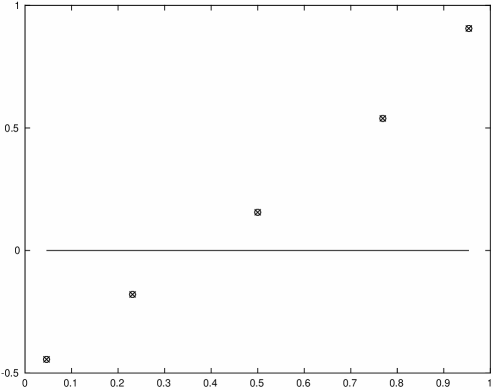
Figure 13: Course mesh plot of exact & computed Wiener–Hopf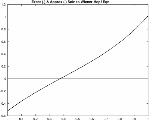

Figure 14: Fine mesh plot of exact & computed Wiener–Hopf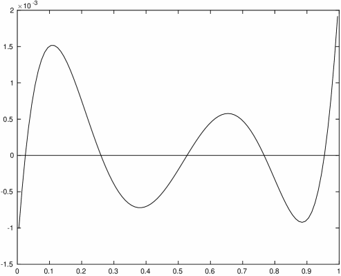

Figure 15: Fine mesh plot of error of Wiener–Hopf

References

[B] T. Bromwich, Normal coordinates in dynamical systems, Proc. London Math. Soc., 15 (1916) 401–448.

[BS] G. Baumann & F. Stenger, Fractional Fokker–Planck Equation, Mathematics 5 (2017) 1–19.

[DS] G. Dahlquist & F. Stenger, Approximate solution of ODE via approximate indefinite integration, submitted.

[GH] W. Gautschi & E. Hairer, A conjecture of Stenger in the theory of orthogonal polynomials, submitted.

[GR] K.E. Gustafson & D.K.M. Rao, Numerical Range: The Field of Values of Linear Operators and Matrices, Springer–Verlag (1996).

[H] S. Haber, Two Formulas for Numerical Indefinite Integration, Math. Comp., v. 60 (1993) 279­296.

[HX] L. Han & J. Xu, Proof of Stenger’s Conjecture on Matrix $I^{(-1)}$ of Sinc Methods, J. Comp. Appl. Math., 255 (2014) 805–811.

[K] R.B. Kearfott, A Sinc Approximation for the Indefinite Integral, Math. Comp., V. 41 (1983) 559–572.

[L] P. Lax, Functional Analysis, Wiley & Sons (2002).

[Fc] F. Stenger, Collocating Convolutions, Math. Comp., 64 (1995) 211–235.

[N] A. Naghsh–Nilchi, Sinc Convolution Method of Computing Solutions to Maxwell’s Equations, Ph.D. thesis (1997). quarter, 1997.

[P] E. Post, Generalized differentiation, Trans. AMS 32 (1930) 723-781.

[SA] F. Stenger, SÅ. Gustafson, B. Keyes, M. O’Reilly, & K. Parker, ODE – IVP – PACK via Sinc Indefinite Integration and Newton’s Method, Numerical Algorithms 20 (1999) 241–268.

[Si] F. Stenger, Numerical Methods Based on the Whittaker Cardinal, or Sinc Functions, SIAM Rev. 23 (1981) 165–224.

[Sp] F. Stenger, Numerical methods based on Sinc and analytic functions, Springer–Verlag (1993).

[Sc] F. Stenger, Handbook of Sinc numerical methods, CRC Press (2011).

[Srh] F. Stenger, A proof of the Riemann hypothesis,
http://arxiv.org/abs/1708.01209

[STB] F. Stenger, D. Tucker & G. Baumann, Solution of Navier–Stokes on ${\mathbf{R}}^{3}\times(0,T)$, Springer–Verlag (2016).

[SKB] F. Stenger, V. Koures & K. Baumann, Computational Methods for Chemistry and Physics, and Schrödinger $3+1$, In: John R. Sabin and Remigio Cabrera-Trujillo, editors, Advances in Quantum Chemistry, Burlington: Academic Press, 71 (2015) 265-298.

[Y] T. Yamamoto, Approximation of the Hilbert transform via use of Sinc convolution, ETNA 23 (2006) 320–328.