Parameter Optimization and Uncertainty Analysis of $\mathtt{FREYA}$ for Spontaneous Fission

Abstract

In this paper we report on an effort to determine an optimal parameter set for the complete event fission model $\mathtt{FREYA}$ to reproduce spontaneous fission of ²⁵²Cf(sf), ²⁴⁴Cm(sf), ²³⁸Pu(sf), ²⁴⁰Pu(sf), ²⁴²Pu(sf), and ²³⁸U(sf). Earlier studies have partially optimized the event-by-event fission model $\mathtt{FREYA}$ with respect to the available experimental data using brute force computational techniques. We have confirmed and expanded these results using a least-squares minimization based on the simulated annealing approach. We have also developed a more complete statistical picture of this optimization, consisting of a full correlation matrix for the parameters utilized by $\mathtt{FREYA}$. The newly improved parameter values themselves, along with this correlation matrix, have led to a more well-developed physical picture of the fission process.

1 Introduction

Though nuclear fission has influenced society in significant ways, the fission process itself is still not understood in great detail. Nevertheless, we can produce a complete fully-correlated physically-consistent description of fission. The Fission Reaction Event Yield Algorithm ($\mathtt{FREYA}$) fission model is designed to serve this purpose in a physically-complete fashion with a relatively modest computational footprint. While our main focus here is on ²⁵²Cf(sf), we also present optimized parameters for all spontaneously fissioning nuclei in the event-by-event simulation code $\mathtt{FREYA}$ [1, 4, 2, 3, 5, 6]. $\mathtt{FREYA}$ generates samples of complete fission events, including the full kinematic information for the two product nuclei, as well as the emitted neutrons and photons. It was designed to quickly generate large numbers of events. $\mathtt{FREYA}$ is also a published code [5, 6], In this work we concern ourselves with improving the $\mathtt{FREYA}$ input parameters by global optimization and considering the physical implications of the resulting parameter values. We also discuss the areas in which experimental data is lacking for this type of comparison.

The events generated by $\mathtt{FREYA}$ depend on five physics-based parameters. For a given choice of these five parameters, the results can be compared to existing experimental data and evaluations in order to determine how effective each choice is at describing all the data. This work was carried out using multiple different numerical optimization techniques in order to determine the most efficient and effective methodology. We make a full statistical analysis, including variances and covariances. In this paper we find the best possible set of the input parameters for describing all the spontaneous fission data for each isotope.

In Sec. 2 we describe the parameters we optimize in $\mathtt{FREYA}$. Sec. 3 discusses the numerical methods used to perform the optimization, while Sec. 4 identifies the data employed in the fits. Sections 5 and 6 provide the results and their interpretation, as well as a comparison between the resulting parameter values to those previously used. We compare results to the data for specific ²⁵²Cf(sf) observables in Sec. 7. Comparisons to other isotopes can be found in the Appendix.

2 $\mathtt{FREYA}$ parameter description

In this section we briefly discuss the process of nuclear fission as implemented in $\mathtt{FREYA}$. We also identify and provide a physical interpretation of the five parameters required by $\mathtt{FREYA}$.

The fission process begins when a specified initial compound nucleus splits into two fragment nuclei, typically one light and one heavy, which we denote by $L$ and $H$ respectively for each fragment pair. The corresponding $Q$-value is given by $Q=M_{0}c^{2}-M_{L}c^{2}-M_{H}c^{2}$ for spontaneous fission. The fragment yields as a function of fragment mass and the total kinetic energy of the fragments, TKE, as a function of heavy fragment mass, $A_{H}$, are sampled from data. From the fission $Q$ value and the sampled TKE we determine the total excitation energy at scission, $E_{\text{sc}}^{*}$, by energy conservation. The excitation energy $E_{\text{sc}}^{*}$ is available for both statistical, $E_{\text{stat}}$, and rotational, $E_{\text{rot}}$, excitation of the fragments. These two quantities are related by:

$$E_{\text{sc}}^{*}=Q-\overline{\text{TKE}}=E_{\text{stat}}+E_{\text{rot}}\ .$$ (1)

The level density parameter $a\approx A_{0}/e_{0}$  [4], for some constant $e_{0}$, determines a “scission temperature” $T_{\text{sc}}$ from the relation:

$$E_{\text{sc}}^{*}=aT_{\text{sc}}^{2}\ .$$ (2)

This $e_{0}$ is the first parameter required by $\mathtt{FREYA}$, and is usually around $10/\textrm{MeV}$ [6]. Note that, while Eq. (2) relates $a$ to the scission temperature, the level density parameter $a$ is also employed for all neutron emission during the fission process.

In addition to the mean angular momenta of the fragment given by the overall rigid rotation around the scission axis, there are also fluctuations around this value attributed to the wriggling and bending modes [9] that contribute to $E_{\text{rot}}$. The relative degree of these fluctuations is given by

$$T_{S}=c_{S}T_{\text{sc}}\ .$$ (3)

The ratio of the fluctuation temperature $T_{S}$ to the scission temperature $T_{\text{sc}}$, $c_{S}$, is our second parameter. It is clear that this must be non-zero. If it were zero, there would be no fluctuations and the only angular momentum present in the fragments would be that dictated by the rigid rotation before scission. In the case of spontaneous fission, this would mean that the fragments have no angular momentum, which is not the case. The default value used in the most recently published version of $\mathtt{FREYA}$ is $c_{S}=0.87$ [6, 7]. See [9] for more details on the addition of angular momentum to $\mathtt{FREYA}$.

The statistical excitation energy, $E_{\text{stat}}$, is initially partitioned as $E_{\text{stat}}=\acute{E}_{L}^{*}+\acute{E}_{H}^{*}$ where the $*$ indicates that the statistical excitation is initially partitioned according to the level density parameters. This would only be completely accurate if the fragments were in mutual thermal equilibrium. However, since we know that the light fragment emits more neutrons on average, we modify the partition via the third parameter, $x$:

$$\overline{E}_{L}^{*}=x\acute{E}_{L}^{*}\ , \overline{E}^{*}_{H}=E_{\text{stat}}-\overline{E}_{L}^{*}\ ,$$ (4)

assumed to be greater than $1$. A value around $1.1-1.3$ is typically found [7, 8].

As noted in Eq. (2), the average fragment excitation energy is proportional to the temperature, i.e. $\overline{E_{i}}^{*}\propto T_{i}^{2}$. The variance of this excitation is given by:

$$\sigma_{E_{i}}^{2}=c\overline{E_{i}}^{*}T_{i}\ .$$ (5)

Therefore we have an energy fluctuation, written $\delta E_{i}^{*}$, on both the heavy and light fragments. This fluctuation is sampled from a normal distribution of variance equal to $2c\overline{E_{i}}^{*}T_{i}$. In particular, the excitation energy of each fragment is adjusted to be $E_{i}^{*}=\overline{E_{i}}^{*}+\delta E_{i}^{*}$. Therefore we can understand the factor $c$, our fourth parameter, as controlling the truncation of the normal distribution at the maximum available excitation. It primarily affects the neutron multiplicity distribution and was assumed to take a value $c\sim 1$. We maintain energy conservation by

$$\text{TKE}=\overline{\text{TKE}}-\delta E_{L}^{*}-\delta E_{H}^{*}\,\,.$$ (6)

Finally, to ensure reproduction of the measured average neutron multiplicity $\overline{\nu}$, we allow the value of the average total kinetic energy to shift by a small amount $d\text{TKE}$. The measured data have often unquantified systematic uncertainties or, in some cases, low statistics.

The ranges considered for these parameters can be found in Table 1. While the range for $c$ is listed as $1-3$, for some isotopes we allow this range to expand. Since this parameter controls the width of the neutron multiplicity distribution, for isotopes which are known to have a comparatively narrow distribution, we allow the parameter to vary below $1$ to $0.8$. In addition, for isotopes with a comparatively wide distribution relative to their average multiplicity we allow $c$ to be as large as $4$.

We note that there are two detector-based photon-related parameters in $\mathtt{FREYA}$, $g_{\text{min}}$, the minimum detected photon energy, and $t_{\text{max}}$, the length of the time measurement. Because these are unique to each measurement, they are not counted as tunable parameters. They do however have some effect on the photon multiplicity and energy per photon [11]. The fits use the values of $g_{\text{min}}$ and $t_{\text{max}}$ appropriate for the data included in the fits.

$e_{0}\,(/{\rm MeV})$	$x$	$c_{S}$	$c$	$d\text{TKE}\,({\rm MeV})$
$7\text{ - }12$	$1.0\text{ - }1.5$	$0.5\text{ - }1.5$	$1\text{ - }3$	$-5\text{ - }5$

Table 1: Ranges of parameters considered in the optimization.

3 Computational methods

Figure 1: (Color online) (a) Contour plot of $\chi^{2}$ relative to various parameter values for ²⁵²Cf(sf) for the full range of tested parameters. (b) Contour zoomed in to focus around optimized parameter values.

For each set of five parameters, we generate sets of $1,000,000$ events. The output from the generated events contains the full kinematic information for the fragments and the emitted neutrons and photons. We use this kinematic information to calculate physical observable which are then compared to measured data. In this study, the quantities we extracted included the average neutron multiplicity, $\overline{\nu}$; the second and third moments of the neutron multiplicity, $\nu_{2}$ and $\nu_{3}$ respectively; the neutron multiplicity distribution, $P(\nu)$; the average neutron multiplicity as a function of the total kinetic energy, $\nu({\rm TKE})$, and as a function of fragment mass, $\nu(A)$; the neutron energy spectrum, $N(E)$; the average photon multiplicity, $\overline{N}_{\gamma}$; the photon multiplicity distribution, $P(N_{\gamma})$; and the average energy per photon $\overline{\epsilon}_{\gamma}$.

The moments of the multiplicity distribution are defined as

$$\nu_{n}=\sum_{n}\frac{\nu!}{(\nu-n)!}P(\nu)$$ (7)

where

$$\nu_{1} = \overline{\nu}=\langle\nu\rangle\,\,,$$

$$\nu_{2} = \left\langle\nu\left(\nu-1\right)\right\rangle\,\,,$$

$$\nu_{3} = \left\langle\nu\left(\nu-1\right)\left(\nu-2\right)\right\rangle\,.$$ (8)

These moments numerically encapsulate the shape of the neutron multiplicity distribution. After calculating these observables from the $\mathtt{FREYA}$ output, they are compared with available experimental data and evaluations. Unfortunately, not all of these observables are available for many of the isotopes of interest, as we discuss later. More information on the sources and quality of these data can be found in Sec. 4.

The $\mathtt{FREYA}$ output is compared to the data, and for each observable the reduced $\chi^{2}$, $\chi_{0}^{2}$ is calculated as

$$\chi^{2}_{O}=\frac{1}{n-5}\sum_{i=1}^{n}\frac{\left(O_{i}-E_{i}\right)^{2}}{\sigma_{i}^{2}}$$ (9)

where $i=1,\dots,n$ runs over the bins of the distribution; $O_{i}$ is the value of the observable returned by $\mathtt{FREYA}$ for the given bin; $E_{i}$ is the experimental result; and $\sigma_{i}$ is the experimental uncertainty on $E_{i}$. The reduced $\chi_{0}^{2}$ for the observable is found by dividing the sum over all bins by the number of degrees of freedom, $n-5$, for the five physics-based parameters we are fitting. For single valued observables such as $\overline{\nu}$, we simply take $\chi_{O}^{2}=\left(O-E\right)^{2}/\sigma^{2}$.

The total $\chi^{2}$ is the sum over all observables where data are available,

$$\chi^{2}=\sum_{O}\chi^{2}_{O}\,\,.$$ (10)

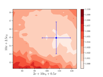
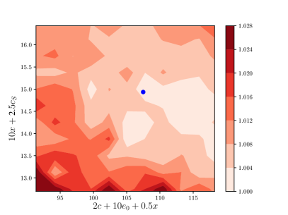
This total $\chi^{2}$ is treated as the return value of an objective function. In Fig. 1 we plot the following: first we take the sum of the reduced $\chi^{2}$ values for a linear combinations of the parameters. Then we find the lowest such value, and plot the ratio of all of the values to this value. These plots show us merely one particular two dimensional projection of the five-dimensional parameter space. The particular linear combination of parameters was chosen by-eye to best illustrate the nature of the parameter space we are working in.

Preliminary work in Ref. [7] used a grid-search method where every potential combination of parameters was tested. However, in a five-dimensional space with a reasonably fine mesh, the grid search technique is unwieldy and very computationally intensive. We have therefore also used alternative methods and confirmed that our alternate methodology agreed with the earlier used grid search approach used earlier.

Fig. 1 shows that the objective function displays many local minima which are neither global minima, nor physically relevant. Therefore, we cannot employ a simple algorithm, such as gradient descent, because it can easily fall into such local minima. We have instead employed the so-called simulated annealing method [12]. The motivation for such an algorithm is to inject a certain amount of randomness into the process to allow for the procedure to occasionally jump in a seemingly “worse” direction in order to move out of a potential local minimum and eventually find the global solution. We provide a rough description of the algorithm now.

The simulated annealing algorithm first generates a random solution, calculates its cost using an objective function, generates a random neighboring solution, calculates the cost of this new solution with the same objective function, and then compares these costs using an acceptance probability function. The acceptance probability is calculated by comparing the difference of the two costs with the so-called temperature, $T$. The parameter $T$ is initially equal to unity, and is decreased to a new value, $T^{\prime}$, after each iteration of the algorithm by employing a scale factor $\alpha$,

$$T^{\prime}=\alpha T\,\,.$$ (11)

The factor $\alpha$ is usually greater than $0.8$, and is always less than $1$. The temperature allows for the algorithm to become less stochastic as the number of iterations is increased. The value returned by the acceptance probability function is then compared to a randomly generated number to determine whether the new solution is accepted. As a result, when the algorithm compares the costs of these two solutions, there is a certain probability that, even if the new solution is worse, it still might be accepted. This helps prevent the algorithm from sinking into a local minimum. The process is repeated until an acceptable solution is found.

In our particular situation, the solutions consist of values of the $5$ parameters and the objective function is the corresponding value of the $\chi^{2}$ from Eq. (10). We define the acceptance probability function of two uncertainties, e.g. $\chi_{0}$ and $\chi_{1}$, for two different parameter sets as

$$\exp\left(\frac{\chi_{0}-\chi_{1}}{\chi_{0}T}\right)$$ (12)

where $T$ is the temperature defined in Eq. (11). Overall, this optimization procedure proved to be the most successful. Gradient descent was successful when the initial guess was guided according to physical intuition. However, simulated annealing was able to determine the global solution without this external help. We also investigated the robustness of this algorithm with respect to the factor $\alpha$ used to lower the temperature. The solution was found relatively reliably for all values of $\alpha$ between $0.85$ and $1$. Below $\alpha=0.85$ the process was still largely successful, but not to the same degree. After finding the general range of the global solution, our simulated annealing algorithm then completes a grid search in a small region surrounding our potential solution to obtain the final minimum with high precision.

4 Data Employed in the Optimization

As noted in Sec. 3, all of the optimization procedures rely on an objective function which computes how closely the $\mathtt{FREYA}$ output reproduces available experimental data. We now discuss in some detail the source and quality of the data for ²⁵²Cf(sf). Though the available data for ²⁵²Cf(sf) are quite extensive, we still were cautious in our selection to avoid fitting to out-of-date or low quality data. We fit the ²⁵²Cf(sf) parameters to all eight observables mentioned in the previous section.

We note that ²⁵²Cf(sf) is the only isotope we consider that has data available for all observables used in the optimization. Thus the parameters for ²⁵²Cf(sf) are the most constrained out of all the fits performed.

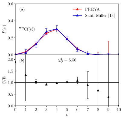
The observed neutron multiplicity distribution $P(\nu)$ is taken from Ref. [13], an evaluation of the prompt neutron multiplicity distributions for the spontaneous fission of a number of isotopes. This consensus resource combines all of the reliable direct sources of data available at this time. We also employ this evaluation for the full distribution $P\left(\nu\right)$, as well as the average neutron multiplicity, $\overline{\nu}$, and the second and third moments, $\nu_{2}$ and $\nu_{3}$, which are defined in Eq. (8). We have chosen to use $\overline{\nu}$ in addition to the actual distribution, because the parameters in $\mathtt{FREYA}$ are capable of shifting $\overline{\nu}$ explicitly, as well as changing the shape of $P\left(\nu\right)$, as described in Sec. 2. Note that for the optimization, we use the square root of the uncertainty given in the evaluation since when we used the reported uncertainty, it was so low it dominated the optimization.

We have used the data from Ref. [14] for the neutron multiplicity as a function of fragment mass, $\nu(A)$. See Ref. [14] for more experimental specifics. While Ref. [15] also measures $\nu(A)$, these data are not used in the optimization procedure. We do however compare $\mathtt{FREYA}$ to this result in Sec. 7. These two data sets are very similar, so the decision between them was largely inconsequential in terms of the fit.

We take the neutron multiplicity as a function of TKE from Ref. [16]. Since these data are from 1988, this set is rather dated. However, this work includes a thorough and honest statistical analysis of the results which yields reliable uncertainties. While Ref. [15] includes a more recent measurement of $\nu(\text{TKE})$, it agrees within uncertainties with Ref. [16] except in regions where the TKE is either very low or very high and is thus of low statistical significance. We compare the $\mathtt{FREYA}$ results to both data sets in Sec. 7.

The prompt fission neutron energy spectrum is taken from the Mannhart evaluation [17]. While also somewhat dated, it is a well-established evaluation. We have used the non-smoothed data, which are presented as the ratio to a Maxwellian distribution of temperature $T=1.32$  MeV. We have multiplied the evaluation by the Maxwellian at the center of each energy bin to obtain the prompt fission neutron spectrum directly. There is also a smoothed version of this spectrum which we have not used here because the non-smoothed version provides an uncertainty while the smoothed spectrum does not. The disadvantage of using this version is the fact that there is a slight kink around 0.1 MeV in the Mannhart spectrum.

Finally, the photon multiplicity distribution, average photon multiplicity, and average photon energy are taken from Ref. [18], measured in 2012 using the DANCE array. See Ref. [18] for more details on this analysis.

We now briefly discuss the data used in fitting the other spontaneously fissioning isotopes in $\mathtt{FREYA}$. Far fewer data are available for these. The optimizations for ²⁴⁰Pu(sf) and ²⁴²Pu(sf) were completed using the neutron multiplicity distribution, average neutron multiplicity, average photon multiplicity, and average photon energy. The neutron multiplicity distribution and its moments were taken from Ref. [13]. Indeed, evaluations from Ref. [13], available for all spontaneously fissioning isotopes included in $\mathtt{FREYA}$ so far, were at times the only data available. The average photon multiplicity and energy for ²⁴⁰Pu(sf) and ²⁴²Pu(sf) both come from Ref. [19]. These data, taken in 2016, are the most recent of all the data used in the optimization. There is also a prompt fission neutron spectrum available for ²⁴⁰Pu(sf) [20]. However, we have chosen not to use these data for the optimization due not only to the limited neutron energy range but also to the questionable quality of the data: the ²⁵²Cf(sf) neutron spectrum in Ref. [20] is in disagreement with the Mannhart spectrum [17].

The neutron multiplicity distribution, average neutron multiplicity, and second and third moments of the distribution for ²⁴⁴Cm(sf) are also available from [13]. We also fit to the neutron multiplicity as a function of fragment mass, take from Ref. [21]. These data only have uncertainties for some values of $A$. These uncertainties are around $0.15$, so we took this to be the default uncertainty for the values of $\nu(A)$ without one. We have done this because some value of uncertainty is required for the calculation of $\chi^{2}$. Finally we use the neutron spectrum from Ref. [22]. Reference [22] also has a neutron spectrum for ²⁴²Pu(sf) but we choose not to use it in the optimization due to quality issues.

The only available data for ²³⁸U(sf) and ²³⁸Pu(sf) are the neutron multiplicity distribution, the average neutron multiplicity, and the second and third moments of the distribution from Ref. [13].

5 Fit Results

We have confirmed the previous ²⁵²Cf(sf)fit results [7] within a reasonable margin, produced uncertainties, and calculated correlation matrices for the parameters. In Table 2 we list our optimized parameter values for ²⁵²Cf(sf). These results are consistent with the default values based on physical intuition given in Sec. 2.

	$e_{0}$	$x$	$c$	$c_{S}$	$d\text{TKE}$
	$(/\textrm{MeV})$				$({\rm MeV})$
$y$	$10.429$	$1.274$	$1.191$	$0.875$	$0.525$
$\sigma_{y}$	$\pm 1.090$	$\pm 0.187$	$\pm 0.362$	$\pm 0.020$	$\pm 0.078$
$y$[7]	$10.37$	$1.27$	$1.18$	$0.87$	$0.52$

Table 2: The optimized parameter set for ²⁵²Cf(sf) along with the previous values of the parameters from [7].

The optimized values for ²⁵²Cf(sf) from the preliminary optimization in Ref. [7] are shown in table 2. There is some difference between our results and those of Ref. [7] because we employ some different data sets, as well as a slightly different optimization scheme, as described in Sec. 3. While some preliminary work was also done for ²⁴⁰Pu(sf), we provide the first complete analysis for this isotope, as well as the other spontaneously fissioning isotopes in $\mathtt{FREYA}$.

We calculate the probability as a function of the $\chi^{2}$, as well as the expectation values according to

$$P(\vec{y}) \equiv\left(\chi^{2}(\vec{y})\right)^{n/2-1}e^{-\chi^{2}(\vec{y})}\ ,$$ (13)

$$\left\langle y_{i}\right\rangle =\int y_{i}\,P(\vec{y})\,d^{5}\vec{y}\ ,$$ (14)

$$\left\langle y_{i}y_{j}\right\rangle =\int y_{i}y_{j}\,P(\vec{y})\,d^{5}\vec{y}\ ,$$ (15)

where $\vec{y}$ denotes the $5$-dimensional vector containing the $5$ parameter values. We integrate over the parameter ranges. Here $n$ is the number of degrees of freedom for all observables. The variance and covariance of the parameters are defined as

$$\sigma_{y_{i}}^{2}=\left\langle y_{i}^{2}\right\rangle-\left\langle y_{i}\right\rangle^{2} \sigma_{y_{i}y_{j}}=\left\langle y_{i}y_{j}\right\rangle-\left\langle y_{i}\right\rangle\left\langle y_{j}\right\rangle\,\,.$$ , (16)

The correlation matrices in Table 3 are readily calculated as

$$\rho_{ij}=\frac{\sigma_{y_{i}y_{j}}}{\sigma_{y_{i}}\sigma_{y_{j}}}\ .$$ (17)

While Eqs. (13)-(17) provide analytic definitions of these quantities, we have numerically calculated the results in Table 3 using a Hessian. In particular, we construct a function representing the logarithm of the probability of $\vec{y}$ and then calculate the Hessian matrix at the optimal point using the parameter uncertainties from Table 2. The negative of the inverse of this matrix is then the covariance matrix. We use Eq. (17) to extract the correlation coefficients displayed in the tables.

	$e_{0}$	$x$	$c$	$c_{S}$	$d\text{TKE}$
$\begin{matrix}e_{0}\\ x\\ c\\ c_{S}\\ d\text{TKE}\end{matrix}$	${\hbox{$\left\{\vbox to35.0pt{}\right.\n@space$}}\begin{matrix}1.0\\ -0.032\\ -0.737\\ 0.924\\ -0.695\end{matrix}$	$\begin{matrix}-0.032\\ 1.0\\ -0.261\\ 0.557\\ 0.213\end{matrix}$	$\begin{matrix}-0.737\\ -0.261\\ 1.0\\ -0.423\\ 0.458\end{matrix}$	$\begin{matrix}0.924\\ 0.557\\ -0.423\\ 1.0\\ -0.673\end{matrix}$	$\begin{matrix}-0.695\\ 0.213\\ 0.458\\ -0.673\\ 1.0\end{matrix}{\hbox{$\left\}\vbox to35.0pt{}\right.\n@space$}}$

Table 3: Correlation coefficients for ²⁵²Cf(sf).

In Fig. 1 we present contour plots of the $\chi^{2}$ for different values of the parameters. We vary the linear combinations listed on the axes and fix all parameters which are not listed to their central values. These plots can be interpreted as surfaces in the higher dimensional space which gives us a particular uncertainty for any choice of $5$ parameters. As previously described, the particular linear combinations of parameters was based on physical intuition in order to best illustrate the nature of the parameter space we are working in. The linear combination of parameters on the axes in Fig. 1 was determined by eye according to the contour plots of the individual parameters. We do not show the variance as an error bar in the lower plot, because it effectively fills the entire displayed range.

As discussed in greater detail in Sec. 3, employing a grid search will always find the proper solution by testing every possible combination, whereas the alternative optimization methods attempt to “climb” around these contours in order to find the point of minimum uncertainty. These plots show that there is not always a clear “valley” of minimal uncertainty, and a simple grid approach is very likely to fall into a local minimum.

It is worth addressing the size of the $\chi^{2}$ in our results. Our $\chi^{2}$ is summed over the uncertainty estimate for each bin of the data sets and evaluations we fit to. While this value is very large, this should not suggest that our fit is low quality, see Sec. 3.

While our main focus is on ²⁵²Cf(sf), we also completed the same analysis for ²³⁸U(sf), ²³⁸Pu(sf), ²⁴⁰Pu(sf), ²⁴²Pu(sf), and ²⁴⁴Cm(sf), the other spontaneously fissioning isotopes currently included in $\mathtt{FREYA}$ [6]. These results are listed in Table 4. A comparison of the fits for these isotopes to the data and evaluations used in the fits are available in the Appendix.

While we have determined uncertainties on the parameter values for these isotopes, obtaining reliable correlation matrices for them is difficult. Table 4, which also lists the number of data sets and evaluations used in our fits, makes this obvious. If only a single evaluation is available, as is the case for ²³⁸U(sf) and ²³⁸Pu(sf), it is difficult to say, without other constraints, how changing one parameter with respect to the others would affect the correlation.

	$e_{0}\;(/{\rm MeV})$	$x$	$c$	$c_{S}$	$d\text{TKE}\;({\rm MeV})$	# Data Sets	# Evaluations
238U(sf)
$y$	$10.391$	$1.220$	$0.939$	$0.899$	$-1.375$	0	1 [13]
$\sigma_{y}$	$\pm 0.352$	$\pm 0.071$	$\pm 0.283$	$\pm 0.280$	$\pm 0.727$	-	-
238Pu(sf)
$y$	$10.521$	$1.232$	$1.968$	$0.893$	$-1.408$	0	1 [13]
$\sigma_{y}$	$\pm 0.581$	$\pm 0.221$	$\pm 0.071$	$\pm 0.071$	$\pm 3.424$	-	-
240Pu(sf)
$y$	$10.750$	$1.307$	$3.176$	$0.908$	$-3.219$	1 [19]	1 [13]
$\sigma_{y}$	$\pm 0.138$	$\pm 0.071$	$\pm 0.355$	$\pm 0.023$	$\pm 0.112$	-	-
242Pu(sf)
$y$	$10.018$	$1.144$	$3.422$	$0.911$	$-1.662$	1 [19]	1 [13]
$\sigma_{y}$	$\pm 1.768$	$\pm 0.152$	$\pm 0.341$	$\pm 0.257$	$\pm 0.118$	-	-
244Cm(sf)
$y$	$10.488$	$1.239$	$1.391$	$0.906$	$-4.494$	2 [21, 22]	1 [13]
$\sigma_{y}$	$\pm 1.519$	$\pm 0.148$	$\pm 0.582$	$\pm 0.322$	$\pm 0.167$	-	-
252Cf(sf)
$y$	$10.429$	$1.274$	$1.191$	$0.875$	$0.525$	4 [14, 15, 16, 18]	2 [13, 17]
$\sigma_{y}$	$\pm 1.090$	$\pm 0.187$	$\pm 0.362$	$\pm 0.020$	$\pm 0.078$	-	-

Table 4: Results of the optimization for all spontaneously-fissioning isotopes modeled by $\mathtt{FREYA}$. The best fit values of the five parameters, $y$, and their associated standard deviations, $\sigma_{y}$, are given for each isotope. In addition, the number of data sets and evaluations used for each isotope are indicated, along with the references for these data. Note that in the case of Ref. [13], the evaluation gives the result for multiple observables: $P(\nu)$, $\overline{\nu}$, $\nu_{2}$ and $\nu_{3}$.

6 Interpretation

In this section we develop a physical interpretation for the parameter values obtained in Sec. 5. We have treated all spontaneously-fissioning isotopes in $\mathtt{FREYA}$ individually, with all five parameters allowed to vary independently regardless of how many data sets are available to constrain them. This is not unreasonable because we do not generally expect the parameters to have the same value for all fissioning systems.

The parameters $c$ and $d$TKE, which influence $P(\nu)$ and $\overline{\nu}$, are perhaps best constrained because evaluations of $P(\nu)$ and the values of its moments are available for all isotopes in $\mathtt{FREYA}$. Indeed, for some cases, these are the only available parameter constraints. Because the shape of $P(\nu)$ and its moments affect both $c$ and $d$TKE, and given that $\overline{\nu}$, $\nu_{2}$ and $\nu_{3}$ vary considerably from isotope to isotope, we can expect $c$ and $d$TKE to vary independently as well. We might expect the largest range of variation for these as well.

The other three parameters ($e_{0}$, $x$ and $c_{S}$) have fewer data available to constrain them. The average photon multiplicity and energy per photon can be used to guide the value of $c_{S}$ for ²⁴⁰Pu(sf), ²⁴²Pu(sf), and ²⁵²Cf(sf). We have $\nu(A)$ data to constrain $x$ for ²⁴⁴Cm(sf) and ²⁵²Cf(sf). Finally, we have used spectral data for ²⁴⁴Cm(sf) and ²⁵²Cf(sf) which provides a partial constraint on $e_{0}$. We remark that it is only partial because all parameters influence the prompt fission neutron spectrum. While $e_{0}$ is directly related to the temperature, see Eq. (2) and thus the slope of the prompt fission neutron spectrum, the parameters $c_{S}$, $x$, and $c$ are also related to the temperature, at least indirectly. Recall that $c$ sets the level of thermal fluctuations, Eq. (5); $x$ controls the sharing of excitation energy between fragments, initially related to the level density, Eq. (4); and $c_{S}$ is related to the scission temperature, Eq. (3). Thus these parameters all also influence the spectrum.

We expect $c_{S}$ to be less than unity while we expect $x$ and $c$ to be larger than unity. Since $e_{0}$ is related to the level density parameter, we expect a value of $8-12$ /MeV from other work [23]. We may also expect $d$TKE to vary considerably to make up for a lack of other constraints on the parameters aside from $\overline{\nu}$ and also, because, on some cases the input data used for TKE$(A_{H})$ have either large uncertainties based on low-statistical samples, or no uncertainties given. An examination of the results in Table 4 can give us insight into how well the optimization procedure met our expectations.

The parameter values for the spontaneously fissioning isotopes in $\mathtt{FREYA}$ 2.0.2 [6] were obtained in a far more empirical fashion. The values for ²⁵²Cf(sf) were taken from Ref. [7], obtained by a grid search procedure. Universal values were then assumed for $c_{S}$ and $e_{0}$. (We note that while $e_{0}$ was fixed to the ²⁵²Cf(sf) value from Ref. [7] for neutron induced fission, the value $e_{0}=10.0724$/MeV was retained from $\mathtt{FREYA}$ version 1.0 [5] for the other spontaneously fissioning isotopes.) While one can reasonably assume that $e_{0}$ has a universal value since the nuclear level densities are related to nuclear structure and not reaction dependent, $c_{S}$ was fixed for expedience. The $x$ parameter for ²⁴⁰Pu(sf) in $\mathtt{FREYA}$ 2.0.2 was fixed from experimental analysis of neutron-neutron correlations in Ref. [8], an observable not used in this optimization because it requires full analysis of the detector setup in each case. However, these correlations exhibit strong sensitivity to $x$ [10]. For other spontaneously fissioning isotopes, it was taken to be $\sim 1.2$.

The parameter $c$ was fixed via examination of $P(\nu)$. Finally, $d$TKE was tuned to $\overline{\nu}$ after the other parameter values were fixed. The work in this paper is the first to make a full optimization of all parameters for all isotopes. It is interesting to compare how well this empirical approach compares with the numerical optimization performed in the current paper.

As already noted, we do not expect $c$ and $d\text{TKE}$ to be independent of isotope. As can be seen in Table 4, they are not. The values obtained for $c$ are driven entirely by $P(\nu)$ and its moments. In the cases where $c$ is large, $c>3$, ²⁴⁰Pu(sf) and ²⁴²Pu(sf), it is because despite the low average neutron multiplicity, $P(\nu)$ is broader than might be expected for low $\overline{\nu}$. In such cases, the range of $c$ needs to be increased to match the higher moments of the multiplicity distribution, $\nu_{2}$ and $\nu_{3}$. There is also one exception to the expectation that $c\geq 1$, ²³⁸U(sf). In this case, the evaluated $P\left(\nu\right)$ is actually more peaked than a distribution with $c=1$ for the same $\overline{\nu}$, requiring the fluctuations to be reduced to achieve agreement with the evaluated $P\left(\nu\right)$ and its moments. Note, however, that, within uncertainties, $c$ is still compatible with unity in this case. The values of $c$ in $\mathtt{FREYA}$ 2.0.2 were $0.92$, $1.91$, $3$, $3.4$ and $1.34$ for ²³⁸U(sf), ²³⁸Pu(sf), ²⁴⁰Pu(sf), ²⁴²Pu(sf) and ²⁴⁴Cm(sf) respectively, in addition to the value of 1.18 found in Ref. [7] for ²⁵²Cf(sf). These empirical guesses are very close to the results obtained from our current optimization based on evaluations that explicitly constrain $c$.

Next, as indicated, we expect $d\text{TKE}$ to vary from case to case, independent of isotope. Ideally $d\text{TKE}$ should be zero with a perfect model along with high statistics input yields and $\text{TKE}\left(A_{H}\right)$. This is indeed the case for ²⁵²Cf(sf), a well-measured standard with a high spontaneous fission rate. $d\text{TKE}$ is small for ²⁵²Cf(sf): $d\text{TKE}=0.525$ MeV here and 0.52 MeV in Ref. [7]. We now compare our optimized $d\text{TKE}$ values for the other isotopes studied here with those in $\mathtt{FREYA}$ 2.0.2 [6]: $d\text{TKE}=-1.345$ MeV, $-1.366$ MeV, $-3.071$ MeV, $-1.600$ MeV, and $-4.35$ MeV for ²³⁸U(sf), ²³⁸Pu(sf), ²⁴⁰Pu(sf), ²⁴²Pu(sf) and ²⁴⁴Cm(sf) respectively. These values are in rather good agreement with those found in our optimization. We note that the large range in $d\text{TKE}$ values is expected and does not affect the physical interpretation of the parameters.

It is notable that these values are, in contrast to that for ²⁵²Cf(sf), all negative and the absolute values are considerably larger. A negative value for $d\text{TKE}$ indicates that the reported TKE$(A_{H})$ distribution is too high, reducing the overall available excitation energy for neutron emission. However, the measured fission rates are much lower for other isotopes and large fluctuations exist in the data. In most of these cases, the number of fission events measured was small so that not many events go into each $A_{H}$ bin. $\mathtt{FREYA}$ samples the yields and $\text{TKE}\left(A_{H}\right)$ directly from measured fission fragment data, often with undefined or unquantified systematic uncertainties. Thus the input TKE$(A_{H})$ in $\mathtt{FREYA}$ in these cases are based on low statistics, sometimes without uncertainties on the data, and with unknown systematic errors. Introducing $d\text{TKE}$ is a way to correct for these unknowns as well as offering a means to compensate for any remaining, unquantified, physics effects.

Previously, the value of $c_{S}$ was fixed at $0.87$ for every isotope of $\mathtt{FREYA}$. We can see that our results for ²⁵²Cf(sf) agree with this but the ²⁴⁰Pu(sf) result is somewhat larger. We generally find that the spin temperature is close to the scission temperature, resulting in fragment spins close to the maximum available rotation. We note that there is some correlation between $c_{S}$ and $d\text{TKE}$. While it may be especially weak for ²⁵²Cf(sf), it could be responsible for the differences observed between the values of $d\text{TKE}$ in $\mathtt{FREYA}$ 2.0.2 [24] and Table 4 since changing $c_{S}$ changes $E_{\rm rot}$ which, in turn, modifies $E_{\rm stat}$, thus ultimately affecting $d\text{TKE}$. Increasing $c_{S}$, as for e.g. ²⁴⁰Pu(sf) to 0.908 from 0.87, increases $E_{\rm rot}$. Thus for a fixed scission energy $E_{\rm sc}$ then, $E_{\rm stat}$ is reduced, decreasing the energy available for neutron emission. To keep $\overline{\nu}$ fixed, absent other variation, $d\text{TKE}$ has to decrease. This is seen in Table 4 as $d\text{TKE}$ is now $-3.219$ MeV instead of $-3.07$ MeV. Similar reductions of $d\text{TKE}$ can be seen for increased $c_{S}$ in the other cases studied.

The parameter $x$ controls the distribution of statistical excitation energy between the fragments after scission. It is well established that $x$ is greater than unity based on $\nu(A)$ data and previous measurements of the average neutron multiplicities from the light and heavy fragments respectively. The previous values of $x$ [24] generally assumed $x\sim 1.2$ aside from the value of 1.27 established in Ref. [7] for ²⁵²Cf(sf) and the $1.3$ found for ²⁴⁰Pu(sf) based neutron-neutron angular correlation data [8]. The estimates of $x\sim 1.1-1.2$ for the other spontaneously fissioning isotopes were borne out by our independent fits. Despite the fact that the $x$ range was $1<x<1.5$ in all the fits, with $\nu(A)$ data only available for ²⁴⁴Cm(sf) and ²⁵²Cf(sf), the optimized values are very similar to the default of $x\sim 1.2$ assumed previously.

The values of $e_{0}$ in Table 4 are remarkably similar, between $10$/MeV and $10.75$/MeV for all isotopes, despite the wide range, $7<e_{0}<12$/MeV. This is particularly striking because, of the observables considered, only the prompt fission neutron spectrum shows any direct dependence on $e_{0}$, even though it also depends on every other parameter. For example, increasing $c_{S}$ gives more available excitation energy to neutron emission which could, in principle, increase the average energy per neutron rather than increasing the number of neutrons and thus change the slope of the prompt fission neutron spectrum. Giving a larger share of the excitation energy to the light fragment would also influence the average neutron energy and thus the spectral shape, as would modifying the fluctuations in excitation energy via a change in $c$ because increased fluctuations in statistical excitation, while modifying $P(\nu)$, can also modify the neutron energy. Despite this, $e_{0}$ remains remarkably similar for all cases, even though it was fit independently. Recall that, even though Eq. (2) refers to the temperature at scission, the same equation applies to every neutron emitted throughout the fission process as well. Thus, in turn, $e_{0}$ influences the emission of every neutron even though it only has a visible influence on the neutron spectrum and not on e.g. $\nu(A)$.

It is worth noting, that the results for $e_{0}$, $x$, and $x_{S}$ in Table 4 are all very similar. The similarity of these parameters is an indication that the mechanisms employed in $\mathtt{FREYA}$ are physically relevant. As mentioned in Sec. 2, we allow a larger variation of $c$ for some isotopes because the widths of the neutron multiplicity distributions can vary significantly between isotopes.

We can also gain physical intuition from the results in Table 3. As expected mathematically, these matrices are symmetric with unity along the diagonal. In addition, the off-diagonal values are bounded by unity. A positive correlation between two parameters suggests that, when one of these parameters is raised, in order to maintain agreement with the data, the other must increase as well. A negative correlation suggests that when one is raised, the other needs to decrease to compensate. A correlation with an absolute value close to unity indicates that the relationship between parameters is strong while, when the correlation is close to zero, this relationship is weak.

We now discuss the correlations between the input parameters, starting with the correlation of $e_{0}$ with the other parameters and proceeding across Table 3. The correlation between $e_{0}$ and $x$ is the weakest. This is because the initial excitation energy partition is divided up between the two fragments according to their level densities, as described in Sec. 2. The ratio of the level densities is independent of changes to $e_{0}$. The parameter $x$ is a perturbation on that ratio, resulting in a weak correlation. The correlation between $e_{0}$ and $c$ is large and negative so that, when $e_{0}$ is increased, $c$ decreases. Since $e_{0}$ is related to the fragment energy before neutron emission, see Eq. (2), increasing $e_{0}$ while keeping the energy for neutron emission fixed forces the temperature to increase. Since $c$ is related to the thermal fluctuations in the decaying nucleus, if the temperature increases, then the fluctuations can also increase so that $c$ has to decrease to compensate. The correlation between $e_{0}$ and $c_{S}$ is the strongest of all, near $+1$, implying that $c_{S}$ must increase when $e_{0}$ increases. Again, increasing $e_{0}$ can imply an increase in temperature and a probability of greater neutron emission. To compensate, $c_{S}$ needs to increase to give more rotational energy to the fragments and more photon emission to keep the neutron emission fixed. There is also a relatively strong, negative, correlation between $e_{0}$ and $d$TKE. A higher fragment temperature could either lead to increased neutron emission or emission of higher energy neutrons. If fewer neutrons are emitted with higher average energy, then dTKE would need to decrease to compensate to increase the total excitation energy to increase neutron emission.

There is a relatively weak correlation between $x$ and $c$. Since $x$ adjusts how the statistical excitation energy is divided between the fragments, it primarily affects $\nu(A)$ whereas $c$ adjusts the width of the multiplicity distribution $P(\nu)$. A moderate positive correlation is seen between $x$ and $c_{S}$. If $x$ is increased to give more energy to the light fragment, the average neutron multiplicity can be expected to increase. Thus $c_{S}$ must increase to take more rotational energy and keep the neutron multiplicity constant. The correlation between $x$ and $d$TKE is small and positive so that, if $x$ increases neutron emission, then $d$TKE must increase to compensate and reduce the total excitation energy.

A moderate, negative correlation is seen between $c$ and $c_{S}$. If $c$ increases, $\overline{\nu}$ will decrease so that, for $\overline{\nu}$ to be maintained, the rotational energy, and thus $c_{S}$, has to decrease. On the other hand, the correlation between $c$ and $d$TKE is moderate but positive. If neutron emission increases with increasing $c$, then to increase the total excitation energy to compensate, $d$TKE has to increase also to decrease the neutron multiplicity. Finally, there is a relatively large negative correlation between $c_{S}$ and $d$TKE. If $c_{S}$ is increased, the fragment spin and thus rotational energy increases, taking energy away from that available for statistical neutron emission. Thus $d$TKE has to decrease to give more total excitation energy to the fragments and maintain the value of $\overline{\nu}$.

7 Comparison to Data

Figure 2: (Color online) (a) Neutron multiplicity distribution for ²⁵²Cf(sf) compared to the Santi-Miller evaluation Ref. [13]. Note that for the comparison, we use the square root of the uncertainty given in the evaluation since the reported uncertainty was so low it dominated the optimization. Note that the uncertainty on the $\mathtt{FREYA}$ calculation is the variance of the result, which we then present as a standard deviation. Therefore this should not be interpreted as the range of values we should expect from $\mathtt{FREYA}$. In this particular case, since we are not calculating an average, we instead take this variance to be $1/\sqrt{N}$ where $N$ is the number of observed events in that bin. (b) Ratio of calculated values to evaluation results.

Figure 3: (Color online) The same result as in Fig. 2 for ²⁴⁰Pu(sf).

Figure 4: (Color online) (a) Neutron energy spectrum for ²⁵²Cf(sf) from $\mathtt{FREYA}$ as well as the Mannhart evaluation [17] with a logarithmic scale on the $x$ axis. (b) Ratio of calculated values to evaluation results. A logarithmic scale is used on the $x$-axis in both cases. In (c) and (d) the same results are shown now with a logarithmic scale on the $y$-axis, and a linear scale on the $x$-axis in order to highlight the difference and uncertainty at high energy.

We now use the optimized parameters presented in Sec. 5 to generate a set of one million $\mathtt{FREYA}$ events, and compare this to the data used in our optimization, along with some data which were not included. We present the direct comparisons as well as ratios of the calculated to experimental values (C/E). It is important to note that throughout the section, any uncertainties given on the results from $\mathtt{FREYA}$ arise from calculating the variance arising from the propagation of the uncertainties on the model parameters and are not indicative of any statistical uncertainty in the $\mathtt{FREYA}$ calculation. In cases where there is no relevant variance to calculate, we instead use $1/\sqrt{N}$, where $N$ is the relevant event multiplicity in the bin of a distribution. Especially in this case, this ’uncertainty’ should not be compared to the uncertainty on the experimental data.

$\nu_{n}$	Evaluation	$\mathtt{FREYA}$	C/E
238U(sf)
$\overline{\nu}$	$1.98\pm 0.03$	$2.0\pm 0.94$	$1.01\pm 0.22$
$\nu_{2}$	$2.8743\pm 0.1411$	$2.87\pm 3.37$	$1.0\pm 1.37$
$\nu_{3}$	$2.8219\pm 0.481$	$2.83\pm 9.81$	$1.0\pm 11.71$
238Pu(sf)
$\overline{\nu}$	$2.19\pm 0.07$	$2.17\pm 1.15$	$0.99\pm 0.27$
$\nu_{2}$	$3.8736$	$3.85\pm 4.35$	$0.99\pm 1.26$
$\nu_{3}$	$5.417$	$5.25\pm 10.97$	$0.97\pm 4.1$
240Pu(sf)
$\overline{\nu}$	$2.154\pm 0.005$	$2.22\pm 1.25$	$1.03\pm 0.33$
$\nu_{2}$	$3.7889\pm 0.029$	$4.26\pm 4.88$	$1.12\pm 1.66$
$\nu_{3}$	$5.2105\pm 0.1492$	$6.53\pm 13.3$	$1.25\pm 6.51$
242Pu(sf)
$\overline{\nu}$	$2.149\pm 0.008$	$2.12\pm 1.19$	$0.99\pm 0.3$
$\nu_{2}$	$3.8087\pm 0.036$	$3.79\pm 4.51$	$0.99\pm 1.4$
$\nu_{3}$	$5.3487\pm 0.036$	$5.36\pm 12.13$	$1.0\pm 5.14$
244Cm(sf)
$\overline{\nu}$	$2.71\pm 0.01$	$2.7\pm 1.16$	$1.0\pm 0.18$
$\nu_{2}$	$5.941\pm 0.0188$	$5.95\pm 5.46$	$1.0\pm 0.84$
$\nu_{3}$	$10.112\pm 0.175$	$10.17\pm 16.78$	$1.01\pm 2.75$
252Cf(sf)
$\overline{\nu}$	$3.757\pm 0.01$	$3.74\pm 1.3$	$1.0\pm 0.12$
$\nu_{2}$	$11.9517\pm 0.0188$	$11.94\pm 8.79$	$1.0\pm 0.54$
$\nu_{3}$	$31.668\pm 0.175$	$31.84\pm 39.94$	$1.01\pm 1.59$

Table 5: Average neutron multiplicity and the second and third moments of the neutron multiplicity distribution for all six isotopes in $\mathtt{FREYA}$ compared with the evaluations in Ref. [13]. Note that the uncertainty on the $\mathtt{FREYA}$ calculation is a calculation of the variance of the result, and should therefore not be interpreted as the range of values we should expect $\mathtt{FREYA}$ to return.

Average	Measured	$\mathtt{FREYA}$	C/E
238U(sf)
$\overline{N}_{\gamma}$	$-$	$6.49\pm 2.42$	$-$
$\overline{\epsilon_{\gamma}}\,\text{(MeV)}$	$-$	$0.94\pm 0.87$	$-$
238Pu(sf)
$\overline{N}_{\gamma}$	$-$	$6.47\pm 2.43$	$-$
$\overline{\epsilon_{\gamma}}\,\text{(MeV)}$	$-$	$1.05\pm 0.93$	$-$
240Pu(sf)
$\overline{N}_{\gamma}\text{\cite[cite]{[\@@bibref{Number}{Ober}{}{}]}}$	$8.2\pm 0.4$	$6.6\pm 2.48$	$0.8\pm 0.09$
$\overline{\epsilon_{\gamma}}\text{\cite[cite]{[\@@bibref{Number}{Ober}{}{}]}}\,\text{(MeV)}$	$0.8\pm 0.07$	$1.0\pm 0.91$	$1.24\pm 1.26$
242Pu(sf)
$\overline{N}_{\gamma}\text{\cite[cite]{[\@@bibref{Number}{Ober}{}{}]}}$	$6.72\pm 0.07$	$6.61\pm 2.43$	$0.98\pm 0.13$
$\overline{\epsilon_{\gamma}}\text{\cite[cite]{[\@@bibref{Number}{Ober}{}{}]}}\,\text{(MeV)}$	$0.843\pm 0.012$	$0.96\pm 0.89$	$1.14\pm 1.12$
244Cm(sf)
$\overline{N}_{\gamma}$	$-$	$7.07\pm 2.56$	$-$
$\overline{\epsilon_{\gamma}}\,\text{(MeV)}$	$-$	$1.01\pm 0.93$	$-$
252Cf(sf)
$\overline{N}_{\gamma}\text{\cite[cite]{[\@@bibref{Number}{Ch}{}{}]}}$	$8.14\pm 0.4$	$7.71\pm 2.8$	$0.95\pm 0.12$
$\overline{\epsilon_{\gamma}}\text{\cite[cite]{[\@@bibref{Number}{Ch}{}{}]}}\,\text{(MeV)}$	$0.94\pm 0.05$	$0.91\pm 0.86$	$0.97\pm 0.83$

Table 6: Average photon multiplicity and average energy per photon for all six isotopes in $\mathtt{FREYA}$ compared with experimental data (when available). The data for ²⁵²Cf(sf) comes from Ref. [18] while the data for ²⁴⁰Pu(sf) and ²⁴²Pu(sf) both come from Ref. [19]. Note that the uncertainty on the $\mathtt{FREYA}$ calculation is a calculation of the variance of the result, and should therefore not be interpreted as the range of values we should expect $\mathtt{FREYA}$ to return.

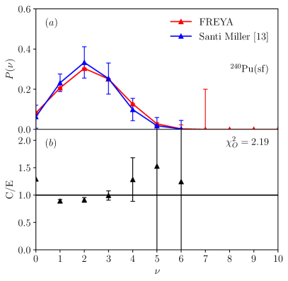
As can be seen in Figs. 2 and 3 we reproduce the neutron probability distribution $P(\nu)$ within very low uncertainty in both cases. As discussed in Sec. 4, the neutron multiplicity distributions are well established for both of these isotopes. Even where we do differ from the result, the uncertainties on C/E are still compatible with unity. We also reproduce the average neutron multiplicity in Table 5 to one or two decimal points, effectively the regime in which we can accurately interpret the $\mathtt{FREYA}$ results. We also note that the neutron multiplicity moments have improved with the new set of parameters over those from Ref. [7]. The moments are important for criticality studies. Note that the uncertainty on the $\mathtt{FREYA}$ calculation is a calculation of the variance of the result, and should therefore not be interpreted as the range of values we should expect $\mathtt{FREYA}$ to return.

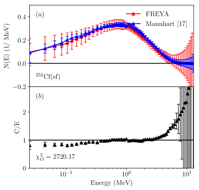
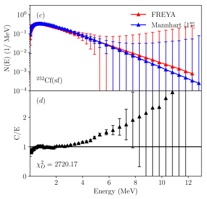
The prompt fission neutron spectrum is compared to the Mannhart evaluation in Fig. 4. We show the results on a logarithmic scale on the $x$ axis in (a) and (b) as well as the $y$ axis in (c) and (d). These particular scales allows us to get a good sense of the behavior of the spectrum in both the low energy regime from $0$ to $1$ MeV, in (a) and (b), as well as the high energy range from $1$ to $12$ MeV, in (c) and (d). $\mathtt{FREYA}$ reproduces this distribution with high accuracy in the low energy range except for the slight kink around $0.1$ MeV present in the non-smoothed version of the Mannhart evaluation, which we employ because it includes uncertainties. There is a more significant deviation in the high energy range, but the range of uncertainty in C/E is consistent with unity for neutron energies above $7$ MeV. It is also important to note that the uncertainties are extremely large in this high-energy region for both the experimental data and the $\mathtt{FREYA}$ output. We note that the $\mathtt{FREYA}$ uncertainties in the high energy tail of the spectrum can be reduced by generating a larger number of events while the uncertainties on the evaluation cannot.

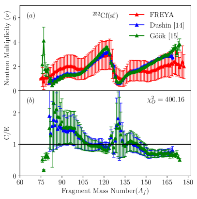
The $\mathtt{FREYA}$ results differ more significantly from the data on the neutron multiplicity as a function of fragment mass, as seen in Fig. 5. This is expected since $x$ is single valued and our fit employs the mass region $105<A<145$. Even though we have only used this well-behaved region for our optimization procedure, it is important to note that the result is still within the uncertainty on C/E, meaning that this result is still statistically successful. We can also compare to experimental data not used in the optimization. In Fig. 5, we show a more recent data set for $\nu(A)$ which also agrees well with $\mathtt{FREYA}$ in the fit region. Note that the uncertainty on the $\mathtt{FREYA}$ calculation is a calculation of the variance of the result, and should therefore not be interpreted as the range of values we should expect $\mathtt{FREYA}$ to return.

Figure 5: (Color online) (a) Neutron multiplicity as a function of fragment mass for ²⁵²Cf(sf) along with experimental data from Refs. [14, 15]. As discussed in Sec. 4, we use the Dushin data in the fit, and provide the Göök data [15] for comparison. Note that the uncertainty on the $\mathtt{FREYA}$ calculation is a calculation of the variance of the result, and should therefore not be interpreted as the range of values we should expect $\mathtt{FREYA}$ to return. (b) Ratio of calculated result from $\mathtt{FREYA}$ to the experimental results.

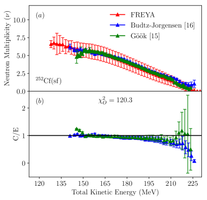
The results for the neutron multiplicity as a function of TKE in Fig. 6 are particularly successful for $160<\text{TKE}<190$ MeV. In the region of low TKE, we see far fewer fragments, so the results in this region are less reliable. Similarly, as we move to higher TKE, while the results begin to differ more, the uncertainty on C/E typically contains unity since there are also fewer events with high TKE. We also show the more recent data, not used in the fit, in Fig. 6. $\mathtt{FREYA}$ actually agrees better with this new data at large TKE because $\nu\left(\text{TKE}\right)\rightarrow 0$ at large TKE.

Figure 6: (Color online) (a) Neutron multiplicity as a function of total kinetic energy for ²⁵²Cf(sf) compared to experimental data from Refs. [15, 16]. As is discussed in Sec. 4, we use the Budtz-Jorgensen data [16] for the fit, and provide the the Göök data [15] for comparison. Note that the uncertainty on the $\mathtt{FREYA}$ calculation is a calculation of the variance of the result, and should therefore not be interpreted as the range of values we should expect $\mathtt{FREYA}$ to return. (b) Ratio of calculated $\mathtt{FREYA}$ result to the experimental results.

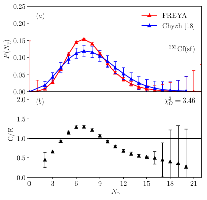
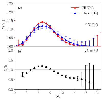
As explained in Sec. 2, the parameters, especially $c$, have a high level of control over the shape of the neutron multiplicity distribution. This is, however, not the case for the photon multiplicity distribution: there is no parameter that has direct control over the width of this distribution as there is for $P(\nu)$. The shape generated by $\mathtt{FREYA}$ in Fig. 7 is narrower than the data. There is an estimated uncertainty of $\pm 1$ in the detected photon multiplicity [25]. If we adjust the $\mathtt{FREYA}$ output to account for multiple scattering [25], the width becomes broader. As we can see in Fig. 7, after adjusting the $\mathtt{FREYA}$ output for multiple scattering, the agreement of $\mathtt{FREYA}$ with the data is considerably improved. As is evident, the uncertainty on C/E is compatible with unity in the high multiplicity range. The average photon multiplicity is also closely recreated. These results can be found in Table 6, along with the average energy per photon.

Figure 7: (Color online) (a) Gamma multiplicity distribution for ²⁵²Cf(sf) along with experimental data from [18] before correcting for multiple scattering. (b) Ratio between the calculated values from $\mathtt{FREYA}$ and the experimental data. (c) Gamma multiplicity distribution for ²⁵²Cf(sf) along with experimental data from [18] after correcting for multiple scattering. (d) Ratio between the calculated values from $\mathtt{FREYA}$ and the experimental data.

8 Conclusions

We have performed a numerical optimization of the $5$ physics-based parameters in $\mathtt{FREYA}$ for all spontaneously-fissioning isotopes so far included. The fits, using simulated annealing to find a global minimum, which agree with our physics intuition, are also in rather good agreement with the empirical values in $\mathtt{FREYA}$ 2.0.2 [6].

The parameters provide good agreement with the data where they are available. We will next apply the fitting procedure we have developed here to neutron-induced fission.

Appendix A ^238,242Pu(sf) and ²³⁸U(sf) neutron multiplicity distributions

In this appendix, we show the neutron multiplicity distributions, $P(\nu)$ resulting from our fits to the ²³⁸U(sf), ²³⁸Pu(sf), and ²⁴²Pu(sf) evaluations by Santi and Miller [13]. The ²⁴⁴Cm(sf) multiplicity distribution is shown in the next section, along with comparisons to other available ²⁴⁴Cm(sf) data.

Figure 8: (Color online) (a) Neutron multiplicity distribution for ²³⁸U(sf) is compared to the Santi-Miller evaluation Ref. [13]. Note that for the comparison, we use the square root of the uncertainty given in the evaluation, since the actual reported uncertainty was so low it dominated the optimization. (b) Ratio of calculated values to evaluation results.

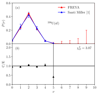
The three isotopes shown here, like ²⁴⁰Pu(sf), as shown in Fig. 3, are characterized by rather low average neutron multiplicities, $\overline{\nu}\sim 2$ for ²³⁸U(sf) and $\overline{\nu}\sim 2.15$ for ^238,240,242Pu(sf). These isotopes are also distinguished by the lack of other data for optimization. While ^240,242Pu(sf) have had recent measurements of the average photon multiplicity and energy per photon, as shown in Table 6, the only data for optimization of the $\mathtt{FREYA}$ parameters for ²³⁸U(sf) and ²³⁸Pu(sf) are the Santi-Miller evaluations of $P(\nu)$ and the corresponding neutron multiplicity moments.

Figure 9: (Color online) (a) Neutron multiplicity distribution for ²³⁸Pu(sf) is compared to the Santi-Miller evaluation Ref. [13]. Note that for the comparison, we use the square root of the uncertainty given in the evaluation, since the actual reported uncertainty was so low it dominated the optimization. (b) Ratio of calculated values to evaluation results.

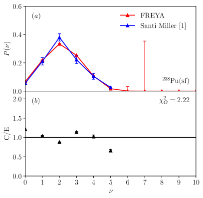
Figure 8 shows the neutron multiplicity distribution for ²³⁸U(sf) compared to the $\mathtt{FREYA}$ calculation. This isotope, with the lowest neutron multiplicity, is especially interesting because it is the only one with $c<1$. Indeed, it is the only one where $\nu_{3}<\nu_{2}$, with $\mu_{2}=2.87$ and $\nu_{3}=2.82$ respectively. With the default value of $c=1$, when the neutron multiplicity is low, $\mathtt{FREYA}$ tends to produce $P(\nu)$ distributions more narrowly peaked than the evaluations, requiring $c\sim 2-3$ for the Pu(sf) isotopes included in $\mathtt{FREYA}$, see Table 4. However, ²³⁸U(sf) is the only isotope where $c=1$ produces a neutron multiplicity distribution wider than the evaluation, requiring $c<1$. With the fitted value of $c=0.939$ in $\mathtt{FREYA}$, there is good agreement with $P(\nu)$ as well as with the moments of the distribution, see Table 5.

Figure 10: (Color online) (a) Neutron multiplicity distribution for ²⁴²Pu(sf) is compared to the Santi-Miller evaluation Ref. [13]. Note that for the comparison, we use the square root of the uncertainty given in the evaluation, since the actual reported uncertainty was so low it dominated the optimization. (b) Ratio of calculated values to evaluation results.

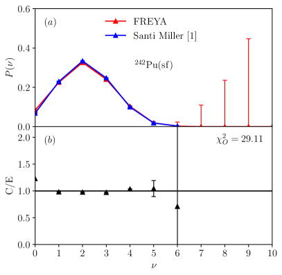
On the other hand, even though $\overline{\nu}$ for the Pu(sf) isotopes is only $\leavevmode\nobreak\ 7.5$% larger than than of ²³⁸U(sf), the higher moments are considerably larger, leading to a broader $P(\nu)$. For all three Pu(sf) isotopes, $\nu_{2}\sim 3.8$ and $\nu_{3}\sim 5.3$. These multiplicity distributions, considerably broader than a default $c=1$ calculation in $\mathtt{FREYA}$, result in the optimized values of $c$ to be $\sim 2-3.4$, see Table 4. In each case, $\nu_{2}$ is approximately 76% larger than $\overline{\nu}$ while $\nu_{3}$ increases by $\sim 40$% over $\nu_{2}$.

The evaluated multiplicity distributions are compared to the optimized $\mathtt{FREYA}$ results in Figs. 9 and 10. The agreement with ²⁴²Pu(sf) and $\mathtt{FREYA}$ is better than that for ²³⁸Pu(sf) where $\mathtt{FREYA}$ underestimates $\nu_{3}$ by 3%.

Appendix B ²⁴⁴Cm(sf) results for $P(\nu)$, $\nu(A)$ and prompt fission neutron spectrum

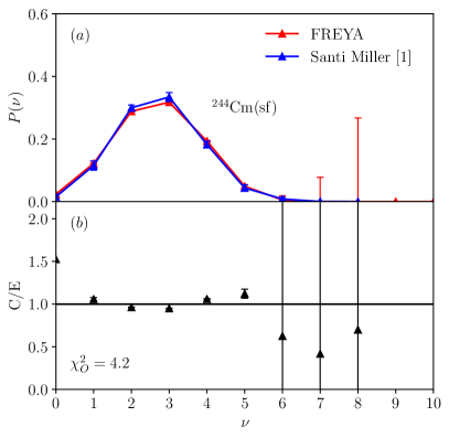
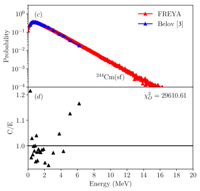
Because ²⁴⁴Cm(sf) has more data available for optimization than the evaluation of $P(\nu)$ and the multiplicity moments, we have collected all the comparisons of the ²⁴⁴Cm(sf) data with $\mathtt{FREYA}$ results in this appendix. While there are data on $\nu(A)$ and the prompt fission neutron spectrum for ²⁴⁴Cm(sf), these data are not of very high quality. Nonetheless, they were useful for constraining the $\mathtt{FREYA}$ parameters and lead to results consistent with the other fits.

We note that the ²⁴⁴Cm(sf) neutron multiplicity is considerably larger than those in Appendix A, $\overline{\nu}=2.71$ relative to $\overline{\nu}\sim 2-2.15$ for ²³⁸U(sf) and Pu(sf). Consequently the behavior of the moments of $P(\nu)$ are more similar to those of ²⁵²Cf(sf): $\nu_{2}/\overline{\nu}=2.19$ for ²⁴⁴Cm(sf) and 3.18 for ²⁵²Cf(sf) while $\nu_{3}/\nu_{2}=1.70$ for ²⁴⁴Cm(sf) and 2.65 for ²⁵²Cf(sf). In the case of the Pu isotopes, $\nu_{2}/\overline{\nu}<2$ and $\nu_{3}/\nu_{2}\sim 1.4$, again emphasizing the relative narrow multiplicity distributions attendant to smaller average neutron multiplicities. The optimal value for $c$ is thus reduced considerably for ²⁴⁴Cm(sf): $c=1.391$, similar to the result for ²⁵²Cf(sf) of $c=1.191$. The comparison with $\mathtt{FREYA}$, shown in Fig. 11, shows good agreement with the evaluation of Ref. [13].

Figure 11: (Color online) (a) Neutron multiplicity distribution for ²⁴⁴Cm(sf) is compared to the Santi-Miller evaluation Ref. [13]. Note that for the comparison, we use the square root of the uncertainty given in the evaluation, since the actual reported uncertainty was so low it dominated the optimization. (b) Ratio of calculated values to evaluation results.

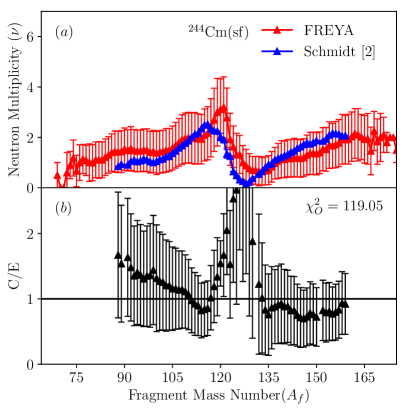
The neutron multiplicity as a function of fragment mass is shown compared to $\mathtt{FREYA}$ in Fig. 12. While the generic sawtooth pattern is recreated well, there are some differences, especially near symmetry where the ‘tooth’ calculated with $\mathtt{FREYA}$ is sharper than that of the data. The peak of $\nu(A)$ of the measured distribution is at a somewhat lighter mass number than in $\mathtt{FREYA}$. Otherwise the agreement with the overall trends of the data away from symmetry. It is worth noting that Ref. [21] made corrections to their ²⁴⁴Cm(sf) data based on a ²⁵²Cf(sf) measurement taken with the same apparatus. The corrected $\nu(A)$, shown here, resulted in a significant backward shift of the light fragment peak near symmetry.

Figure 12: (Color online) (a) Neutron multiplicity as a function of fragment mass for ²⁴⁴Cm(sf) along with experimental data from Refs. [21]. (b) Ratio of calculated result from $\mathtt{FREYA}$ to the experimental results.

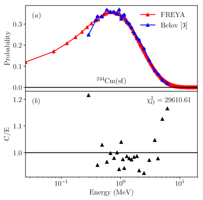
Finally, we compare $\mathtt{FREYA}$ to a measurement of the ²⁴⁴Cm(sf) prompt fission neutron energy spectrum in Fig. 13. The measured energy range is rather narrow, with a good deal of scatter between the points and a drop off of the lowest energy point. Nonetheless the agreement of the data with the calculation is rather good over the common energy interval.

Figure 13: (Color online) (a) Neutron energy spectrum for ²⁴⁴Cm(sf) from $\mathtt{FREYA}$ as well as experimental data from [22] with logarithmic scale on $x$ axis. (b) Ratio of calculated result from $\mathtt{FREYA}$ to the experimental results. In (c) and (d) the same results are shown now with a logarithmic scale on the $y$-axis, and a linear scale on the $x$-axis.

References

- [1] J. Randrup, R. Vogt, Calculation of fission observables through event-by-event simulation, Phys. Rev. C 80 (2009) 024601.
- [2] R. Vogt, J. Randrup, D. A. Brown, M. A. Descalle, and W. E. Ormand, Event-by-event evaluation of the prompt fission neutron spectrum from 239Pu(,f), Phys. Rev. C 85 (2012) 024608.
- [3] R. Vogt and J. Randrup, Event-by-event study of photon observables in spontaneous and thermal fission, Phys. Rev. C 87 (2013) 044602.
- [4] R. Vogt and J. Randrup, Event-by-event study of neutron observables in spontaneous and thermal fission, Phys. Rev. C 84 (2011) 044621.
- [5] J. Verbeke, R. Vogt, and J. Randrup, Fission Reaction Event Yield Algorithm, – For event-by-event simulation of fission, Comp. Phys. Comm. 191 (2015) 178.
- [6] J. Verbeke, R. Vogt, and J. Randrup, Comp. Phys. Comm. 222 (2018) 263.
- [7] R. Vogt, A. Nicholson, J. Randrup, I. Gauld, and S. Croft, Uncertainty Quantification with the Event-by-Event Fission Model FREYA, Proc. 1st ANS Advances in Nuc. Nonpro. Tech. and Policy, Santa Fe, NM, 2016, LLNL-CONF-690741.
- [8] J.M. Verbeke, L.F. Nakae, and R. Vogt, Neutron-Neutron Angular Correlations in Spontaneous Fission of and Phys. Rev. C 97 (2018) 044601.
- [9] J. Randrup and R. Vogt, Refined treatment of angular momentum in the event-by-event fission model , Phys. Rev. C 89 (2014) 044601.
- [10] R. Vogt and J. Randrup, Neutron angular correlations in spontaneous and neutron-induced fission, Phys. Rev. C 90 (2014) 064623.
- [11] R. Vogt and J. Randrup, Improved modeling of photon observables with , Phys. Rev. C 96 (2017) 064620.
- [12] S. Kirkpatrick, C.D. Gelatt and M.P. Vecchi, Optimization by Simulated Annealing, Science 220 (1983) 4598.
- [13] \bibinfoauthorP. Santi and \bibinfoauthorM. Miller, \bibinfotitleReevaluation of Prompt Neutron Emission Multiplicity Distributions for Spontaneous Fission \bibinfojournalNuclear Science and Engineering \bibinfovolume160 (\bibinfoyear2008) 190.
- [14] \bibinfoauthorV. Dushin, \bibinfoauthorF.-J. Hambsch, \bibinfoauthorV. Jakovlev, \bibinfoauthorV. Kalinin, \bibinfoauthorI. Kraev, \bibinfoauthorA. Laptev, \bibinfoauthorD. Nikolaev, \bibinfoauthorB. Petrov, \bibinfoauthorG. Petrov, \bibinfoauthorV. Petrova, \bibinfoauthorV. Petrova, \bibinfoauthorA.S. Vorobyev, et al., \bibinfotitleFacility for neutron multiplicity measurements in fission \bibinfojournalNuclear Instruments and Methods in Physics Research A \bibinfovolume516 (\bibinfoyear2004) \bibinfopages539.
- [15] A. Göök, F.-J. Hambsch, and M. Vidali, Prompt neutron multiplicity in correlation with fragments from spontaneous fission of , Phys. Rev. C 90 (2014) 064611.
- [16] \bibinfoauthorC. Budtz-Jorgensen and \bibinfoauthorH.-H.Knitter, \bibinfotitleSimultaneous Investigation of Fission Fragments and Neutrons in 252Cf(sf) \bibinfojournalNucl. Phys. A \bibinfovolume490 (\bibinfoyear1988) \bibinfopages307.
- [17] \bibinfoauthorW. Mannhart, \bibinfotitleEvaluation of the 252Cf(sf) Fission Neutron Spectrum Between and MeV \bibinfojournalProc. Advisory Group Mtg. Neutron Sources \bibinfovolumeIAEA-TECDOC-410 (\bibinfoyear1986).
- [18] \bibinfoauthorA. Chyzh, \bibinfoauthorC. Y. W., \bibinfoauthorE. Kwan, \bibinfoauthorR. A. Henderson, \bibinfoauthorJ. M. Gostic, \bibinfoauthorT. A. Bredeweg, \bibinfoauthorR. C. Haight, \bibinfoauthorA. C. Hayes-Sterbenz, \bibinfoauthorM. Jandel, \bibinfoauthorJ. M. O’Donnell, \bibinfoauthorJ. L. Ullmann, \bibinfotitleEvidence for the stochastic aspect of prompt emission in spontaneous fission et al., \bibinfojournalPhys. Rev. C \bibinfovolume85 (\bibinfoyear2012) \bibinfopages021601.
- [19] \bibinfoauthorS. Oberstedt, \bibinfoauthorA. Oberstedt, \bibinfoauthorA. Gatera, \bibinfoauthorA. Göök, \bibinfoauthorF.-J. Hambsch, \bibinfoauthorA Moens, \bibinfoauthorG Sibbens, \bibinfoauthorD Vanleeuw, and \bibinfoauthorM. Vidali, \bibinfotitleImpact of low-energy photons on the characteristics of prompt fission -ray spectra \bibinfojournalPhys. Rev. C \bibinfovolume93 (\bibinfoyear2016) \bibinfopages054603.
- [20] \bibinfoauthorZ.A. Aleksandrova, \bibinfoauthorV.I. Bol’shocv, \bibinfoauthorV.F. Kuznetsov, \bibinfoauthorG.N. Smirenkin, \bibinfoauthorM.Z. Tarasko, \bibinfotitleSpectra of the Prompt Neutrons Arising from the Spontaneous Fission of , 244Cm, and 240Pu \bibinfojournalAtomnaya Energiya \bibinfovolume36 (\bibinfoyear1973) \bibinfopages282-285.
- [21] R. Schmidt and H. Henschel, Comparison of the Spontaneous Fission of 244Cm(sf)and 252Cf(sf), \bibinfojournalNucl. Phys. A \bibinfovolume395 (\bibinfoyear1983) \bibinfopages29-43.
- [22] L.M. Belov, M.V. Blinov, N.M. Kazarinov, A.S. Krivokhatskiy, and A.N. Protopopov Spectra of Fission Neutrons of 244Cm(sf), 242Pu(sf), and 239Pu(sf), \bibinfojournalYaderno-Fizicheskie Issledovaniya Reports \bibinfovolume6 (\bibinfoyear1968) \bibinfopages94.
- [23] R. Capote et al., RIPL – Reference Input Parameter Library for Calculations of Nuclear Reactions and Nuclear Data Evaluations, Nucl. Data Sheets 110 (2009) 3107.
- [24] J. M. Verbeke, J. Randrup and R. Vogt, Fission Reaction Event Yield Algorithm: 2.0.2 User Manual, LLNL report LLNL-SM-705798.
- [25] A. Chyzh, private communication.