On the dynamics of Translated Cone Exchange Transformations
Abstract.
In this paper we investigate translated cone exchange transformations, a new family of piecewise isometries and renormalize its first return map to a subset of its partition. As a consequence we show that the existence of an embedding of an interval exchange transformation into a map of this family implies the existence of infinitely many bounded invariant sets. We also prove the existence of infinitely many periodic islands, accumulating on the real line, as well as non-ergodicity of our family of maps close to the origin.
1. Introduction
One of the central problems in dynamical systems is to investigate renormalization of certain classes of maps. We say a map is renormalizable if there is a subset such that the first return map is conjugated to a map in the same family.
Although renormalization of Interval Exchange Transformations (IETs) has been well studied over the past years, renormalization of Piecewise Isometries (PWIs) is still far from understood.
In [1] Adler, Kitchens and Tresser find renormalization operators for three rational rotation parameters for a non ergodic piecewise affine map of the Torus. Lowenstein and Vivaldi [18] gave a computer assisted proof of the renormalization of a family of piecewise isometries of a rhombus with one translation parameter and a fixed rational rotation parameter. These results however rely on fixing the rotation component and heavily restricting other parameters in order to perform computer assisted calculations on cyclotomic fields. Recently, Hooper [14] investigated a two dimensional parameter space of polygon exchange maps, a family of PWIs with no rotation, invariant under a renormalization operation, related to corner percolation and Truchet tillings, where each map admits a return map affinely conjugate to a map in the same family. In [3] the authors show how to construct minimal rectangle exchange maps, associated to Pisot numbers, using a cut-and-project method and prove that these maps are renormalizable. The maps described in these papers are PWIs with no rotational component, exhibiting very particular behaviour among typical PWIs, making it difficult to generalize their techniques.
In this paper we renormalize a particular family of PWIs. Before introducing our family of maps let us define an interval exchange transformation as in [8] (see also [9] and [15]). Let be a natural number and let be an irreducible permutation of , that is, such that for . Let . Consider the points
and the interval partitioned into subintervals for
The interval exchange transformation rearranges according to , that is for where is the translation vector associated to and is given by
We also call a -IET as it is an interval exchange transformation of subintervals.
We now introduce our family of translated cone exchange transformations (TCEs). Consider a partition of the upper half plane into cones , where and for are defined as
We denote by the union of the boundaries of the elements of the partition and by and , respectively, the lines and .
Set , where
Note that we have
| (1.1) |
where is the norm of .
Let be the following family of translation maps
depending on the parameters and with , and .
Consider a permutation and let be the angle associated to the permutation for the cone for . We have
| (1.2) |
Let be the following family of exchange maps
depending on . This map also depends on and as the partition elements depend on these parameters. Note that we have
for , , where is the argument function. Hence exchanges these cones according to the permutation .
From the translation and exchange families of maps we get our family of TCEs, , given by
The dynamics of restricted to is a translation to the left by while the dynamics of restricted to is a translation to the right by , via the action of the translation map . The rest of the cones are all permuted, according to a permutation , by the exchange map and horizontally translated by by the translation map .
Note that TCEs are cone isometry transformations for which the map induced by projection onto the circle at infinity (see [6]) is invertible. is defined on , partitioned into cones by , hence it is a cone exchange transformation. is an interval exchange transformation with interval partition given by and combinatorial data given by the permutation , where , , and , for .
Let us introduce some notation. We define the middle cone of as
the first hitting time of to , as the map given by
and the first return map of to , as the map such that
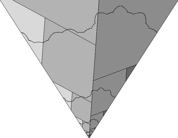
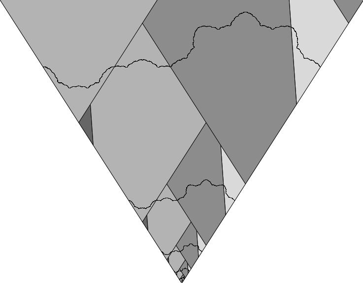
The typical notion of renormalization may not capture all possible self similar behaviour in PWIs. TCEs apparently exhibit invariant regions on which the dynamics is self similar after rescaling. Thus, we say a TCE is renormalizable if , the first return map to described above, is conjugated to itself by a scaling map. In Theorem A we renormalize, in this sense, TCEs for all rotation parameters and for infinitely many translational parameters. We show that for a set of parameters, the first return map under a TCE to , is self-similar by a scaling factor where
Theorem A.
For all , and with , there is an open set containing the origin such that is renormalizable for all , that is
| (1.3) |
As a consequence of this we show that for these parameters is a PWI with respect to a partition of countably many atoms.
We say, as in [7], that is a continuous embedding of an IET into a PWI if is a homeomorphism onto its image and
| (1.4) |
It was proved in [7] that non trivial continuous embeddings of minimal IETs into PWIs, this is, continuous embeddings which are not unions of circles or lines, cannot exist for 2-PWIs and can be at most 3 for any given 3-PWI. In the same paper it is provided numerical evidence for the existence of non trivial embeddings into a 4-PWI belonging to the family of TCEs.
We say a collection of atoms is a barrier for a PWI if is the union of two disjoint connected components , such that
and for any such that and then , for .
For , and , let be the open set in Theorem A. We denote by the subset of such that for all there exist , , and a continuous embedding of into such that , , and the collection
is a barrier for .
In the next theorem we show, as a consequence of renormalization of TCEs, that the existence of one continuous embedding of an IET into a first return map of a TCE, satisfying the property that the image of the embedding is contained in a barrier, implies the existence of infinitely many embeddings of the same IET into , as well as infinitely many bounded and forward invariant regions. This shows in particular that if one non trivial embedding exists then the results from [7] for 2,3-PWIs do not generalize for PWIs with partitions with a higher number of atoms. We prove that for there are infinitely many sets, bounded away from and infinity, which are forward invariant by and that there exist infinitely many continuous embeddings of IETs into .
Theorem B.
Let and with . For all ,
i) There exist sets , which are forward invariant for and such that for all , satisfying , there is an for which .
ii) For all there exist constants such that for all and ,
| (1.5) |
iii) There exist infinitely many continuous embeddings of IETs into .
An horizontal periodic orbit is a periodic orbit , such that there is an for every such that for all . We say is the height of the orbit. An horizontal periodic island is a periodic island that contains an horizontal periodic orbit.
Let denote the set of all such that for some we have
| (1.6) |
Given , let be the set of all such that (1.6) holds for some .
Define the sets (resp. ) of all such that there is a and a such that and (resp. and ). Denote by their union .
In our next theorem we prove that there is a non-empty open set of rotation parameters for which TCEs have infinitely many horizontal periodic islands accumulating on the real line.
Theorem C.
Let , and , for some . There is a non-empty open set such that for all , has infinitely many horizontal periodic islands accumulating on the real line.
As a result we get that for the same parameter set, TCEs are not ergodic in a neighbourhood of the origin.
Theorem D.
Let , , and , for some . If is an invariant set for that contains a neighbourhood of the origin then the restriction of to does not have a dense orbit. In particular is not ergodic.
This paper is organized as follows. In Section 2 we investigate a family of maps related to IETs. In Section 3 we study the sequence of bifurcation points and the bifurcation sequence for the family of maps introduced in the previous section making use of the theory of continued fractions. In Section 4 we introduce two sequences that we designate by dynamical sequences that will be an important tool to prove our main theorems. We derive inductive formulas to compute these sequences. In Section 5 we study the dynamics of the first return map to the middle cone . Finally, in Sections 6 and 7 we prove our main results, theorems A,B, C and D.
2. Bifurcation Points
In this section we study a specific family of maps, closely related to IETs, on the interval with . We will introduce the left and right bifurcation points and bifurcation sets for this family.
Consider the interval and the following family of maps
| (2.1) |
with , and . To simplify notation we will only include the argument when it is necessary, otherwise we just refer to these intervals as for .
Given , consider the region
The next lemma relates iterates of our family of maps with iterates of for some values of .
Lemma 2.1.
For any , and we have
| (2.2) |
for all , where .
Proof.
As we have or . By the definitions of and , in both cases we have . It is direct to see that for we have and thus repeating the previous argument times we get . ∎
We define the first hitting time of to as the map given by
and the first hitting map of to , as the map
For our next lemma we need also to consider the map
Lemma 2.2.
Let and . If with then
| (2.3) |
Proof.
Let and . Consider the map
Let . Define
and
We want now to investigate orbits by of points which are in a small neighbourhood of . We prove the next lemmas.
Lemma 2.3.
Assume that .
i) If and , then for all we have
| (2.4) |
ii) If and , then for all we have
| (2.5) |
Proof.
To simplify notation we denote and . Let us prove i) by induction on . It is clear that (2.4) holds for . We now assume (2.4) holds for and we show it holds for .
It follows from the definitions of and that for , thus or .
If , then as and since we are assuming (2.4) holds for we have . Therefore and since we get
If , then as and since we are assuming (2.4) holds for we have . Therefore and thus
Since , we get that (2.4), holds for and we finish the proof of i).
The proof of ii) is similar to the proof of i) so we omit it. ∎
Given and , we define
| (2.6) |
Lemma 2.4.
Assume , and Then for all we have
| (2.7) |
Moreover, .
Proof.
To simplify notation we denote . We proceed by induction on . It is clear that (2.7) holds for . Now assume (2.7) holds for and we prove it for instead.
As we have . Since we are assuming (2.7) holds for , we get
If , then and thus
Otherwise, if then thus we have if and only if , for and . Therefore by (2.1) we get . This proves (2.7) for .
Since for we have and we finish our proof. ∎
In the beginning of this section we defined the first hitting map of to , as , where is the first hitting time of to . We want now to investigate when is mapped to under and when is mapped to . Note that these are the endpoints of the middle interval . We define the following points and sets.
We say is a right bifurcation point if , is a left bifurcation point if and is a bifurcation point if it is either a left or right bifurcation point.
The left/right bifurcation sets are defined respectively as
and
The main result of this section is the next theorem, relating bifurcation points with the bifurcation sets.
Theorem 2.5.
is a left (resp. right) bifurcation point if and only if (resp. ). Furthermore, and are decreasing functions of and the sets , are discrete with as the only possible point of accumulation.
Proof.
First assume that and . By the definitions of and we have, for , that either or . As , by (2.1) we have for , or . Thus and . Since and this shows and thus . This proves that if is a left bifurcation point, then .
Now assume that . As is irrational we must have , therefore there is such that .
We show, by induction on , that for all and
| (2.8) |
It is clear that (2.8) holds for . We assume it holds for and we prove it for . As we have , and since , this implies that , thus by (2.1) we have that (2.8) must hold for .
Since (2.8) holds for we have and thus for all .
Thus, there is such that . This proves that is a left bifurcation point if and only if . Note that it also shows that is a decreasing function of .
By Lemma 2.4, for all and we have
| (2.9) |
From which follows that If , as , this implies
thus, . Then for all , we have . This proves that if is a right bifurcation point then ,
If , as is irrational we must have , therefore there is an such that .
Now take . By (2.9) we get
hence and we have . Thus, there is a such that . This proves that if then is a right bifurcation point. This proves that is a right bifurcation point if and only if . Note that it also shows that is a decreasing function of .
Since and are decreasing functions of and are also integer valued functions this implies that the sets and are discrete and each has at most one point of accumulation, which has to be . ∎
3. Bifurcation sequence
In this section we study the sequence of bifurcation points for the family (in (2.1)). We will first recall some elements of the theory of continued fractions, and compute the sequence of errors of the semiconvergents of , where and . We will then relate the bifurcation sequence with the theory of continued fractions by showing that this sequence is equal to the sequence of errors of the semiconvergents of .
Throughout this section we assume that is an irrational real number with continued fraction expansion . Consider the sequence of its convergents given by
For all it is well known that
| (3.1) |
Define the sequence of upper semiconvergents of as
which is the sequence of best rational approximations of by above , this is, any other fraction , with , satisfies (see for instance [17]).
The sequence of errors of approximation of the upper semiconvergents smaller than is given by
Analogously, we define the sequence of lower semiconvergents of as
which is the sequence of best rational approximations of by below, this is, any other fraction , with , satisfies .
The sequence of errors of approximation of the lower semiconvergents is given by
Note that and are monotonic sequences of positive real numbers that converge to . Finally, we define recursively the intercalation of and as given by
In the next lemma, we compute explicitly the sequences , and .
Lemma 3.1.
Let , and . For all we have
| (3.2) |
| (3.3) |
and
| (3.4) |
Proof.
Let , be the Fibonacci sequence, given by , and
for .
We begin by proving, by induction on , that for all ,
| (3.5) |
and that for all ,
| (3.6) |
Clearly, (3.5) holds for and (3.6) holds for . Assuming that (3.5) holds for , (3.6) holds for and using , we get The proof of (3.6) is similar to the proof of (3.5) and so we omit it.
Using the fact that is the Fibonacci sequence and some elementary properties of continued fractions it can be easily proved by induction on that
| (3.7) |
Finally we show that (3.2) holds for all . It is clear that and for . Hence (3.2) holds for , and (3.3) holds for .
Now assume (3.2) holds for all and (3.3) for all . We now prove that (3.2) holds for and (3.3) for all . We have
By (3.5) and (3.7), we get . Thus, from (3.8) and (3.9) we have and we get . This proves (3.2) for .
Now, by (3.6) and (3.7), Thus, from (3.8) and (3.9) we have and we get . This proves now (3.3) for .
This completes our proof. ∎
Let for all , and consider the the sequence given by
We have Also let for all , and , for . We define another sequence as
Note that We are interested in studying the bifurcation sets and of . By Theorem 2.5 they are discrete with as the only possible point of accumulation, hence they can be regarded as decreasing sequences, which we now define. Let the right bifurcation sequence be given by
the left bifurcation sequence by
and finally we define recursively the sequence of all bifurcation points of , (it follows from Theorem 2.5 that it is equal to the intercalation of and )
In the next lemma we relate the sequences and with and for all .
Lemma 3.2.
The sequences are equal to , respectively.
Proof.
We first prove by induction on , that , for all . It is clear that . Assuming , we have and , for all . This shows that . As , we get that . This proves that is equal to .
We now prove, by induction on , that , for all . It is clear that , where is the first coefficient in the continued fraction expansion of . Assume . Let be a constant such that . Since , , where and with , by Lemma 2.3, we have for and since and , we have . Combining these, we get
| (3.10) |
By Lemma 2.3 we have for all . Note that . Combining these we get and since is irrational and , this gives
for all . Thus from (3.10), we get that is the largest value can take such that . Since we have , this proves that , and so, that is equal to .
∎
In the next theorem we relate the sequences of errors of upper/lower semiconvergents of with the right/left bifurcation sequences of .
Theorem 3.3.
Assume is an irrational number. The sequences and are equal to and , respectively. Moreover, the associated bifurcation sequence is equal to the sequence of errors of the semiconvergents of .
Proof.
Let be given by
for .
Since is irrational, this shows that we have
From this we get that and for all if and only if for all even
for , and
for .
It is well known (see for instance [17]) that for all . From this it follows that for all even we have
for , and
for . Combining the four expressions above it follows that and for all if and only if for all even we have
| (3.11) |
for , and
| (3.12) |
for .
We now prove, by induction on , that (3.11) and (3.12) hold for all even . Before, we prove by induction on , that
| (3.13) |
for .
We have , thus . Since and , by Lemma 3.2 we have . Thus, (3.13) holds for . Now fix . We assume (3.13) holds for and prove it for instead.
Recall the definition of . We have for any . Note that therefore .
Assume now that . Applying Lemma 2.3 with and we get Since , and we have Combining this we get
which combined with (3.14) gives
| (3.15) |
which is smaller than .
If it is clear from (3.14) that we get (3.15) as well. Since is the sequence of best rational approximations of by below and we have and , we must have
and thus by Lemma 3.2 and (3.15) we have
This completes the proof that (3.13) holds for .
In a similar way, it can be proved that
for all , so we omit the proof.
We now assume that for , we have
| (3.16) |
and that for , we have
| (3.17) |
and prove that we have
| (3.18) |
for all , and
| (3.19) |
for all .
First we prove (3.18), by induction on , for all .
Fix . We assume that (3.18) holds for and prove it for instead. Recall the definition of . With we have that (3.18) is equivalent to and combining these we get
| (3.20) |
From (3.17) we get
for . It follows from this identity and fact that the upper semi-convergents of are its best rational approximations by above, that is the largest integer such that . Recall the definition of . We have for any , thus and by Lemma 3.2, (3.17) and (3.1) we get
Therefore . Applying Lemma 2.3 with and yields
| (3.21) |
By Lemma 3.2, (3.17) and (3.1) we have and since , we get
Combining this identity with (3.20) and (3.21) we have
and since (3.18) holds for we get
| (3.22) |
which is smaller than .
Since is the sequence of best rational approximations of by below and we have and , we must have
and thus by Lemma 3.2 and (3.22) we have
This completes the proof that (3.18) holds for .
We now prove (3.19) by induction on , for all .
Fix . We assume that (3.19) holds for and prove it for instead.
Recall the definition of . With we have that (3.19) is equivalent to and we get
| (3.23) |
From (3.18) we get for . It follows from this identity and from the fact that the lower semi-convergents of are its best rational approximations by below, that is the largest integer such that .
Recall the definition of . We have for any . Thus, By Lemma 3.2, (3.18) and (3.1) we get Therefore . Applying Lemma 2.3 with and we get
Combining the two above identities with (3.23) and since (3.19) holds for we get
| (3.24) |
which is larger than .
Since is the sequence of best rational approximations of by above and we have and , we must have
and thus by Lemma 3.2 and (3.24) we have
This completes the proof that (3.19) holds for .
This proves (3.11) and (3.12) and therefore is equal to the sequence and is equal to the sequence . By definition of and , this implies that as well. This finishes our proof.
∎
Recall our definitions of first hitting time of to and the first hitting map . We want now to relate these to and . This is done in the next theorem.
Theorem 3.4.
Let and let be such that and . Then and Furthermore and .
4. Dynamical sequences
In this section, we introduce the dynamical sequences and . These will be an important tool in order to prove our main theorems and will be later related to the dynamics of our family of maps. We show inductive formulas to compute these sequences and prove that for some choice of parameters is periodic with period at most .
Let
| (4.1) |
and denote
| (4.2) |
We now inductively define our sequences , and depending on the parameters , , and . We will denote these sequences by , and when it is important to stress the dependence on the parameter .
Set
| (4.3) |
Note that as we have . Since is irrational, (see Section 3) is an infinite sequence and converges to . Furthermore by the definitions of and we have . Thus there exists a smallest natural number such that . Set and
For assume we defined , , and and that at least one of the conditions or holds. Set
| (4.4) |
Since is irrational, and (see Section 3) are infinite sequences and converge to , furthermore if , by (4.2) and (4.4) we have , thus there are integers and such that and respectively. We set
If set , else if set
| (4.5) |
where , denotes the integer part of a real number. Finally set
The following lemma characterizes the sequence .
Lemma 4.1.
Given , , and , the sequence with is strictly decreasing and it is either finite or converges to .
Proof.
If or then or , respectively, and by (4.4), . If then, by definition, and thus . This shows that is strictly decreasing and either is finite or for all we have .
We now show that if we have . Assume by contradiction that does not converge to . Since it is strictly decreasing there must exist such that . Since for all , , we must have that either or for infinitely many values of .
Assume the first case holds. Then there is a subsequence such that for all . Since we have in particular that
and by (4.4) thus, we must have and therefore . Hence by the definition of and since , we have
Since is irrational, is an infinite sequence and converges to . Thus there exists an unique natural number such that and by the definition of we must have . Thus we get , which implies that is rational which is a contradiction.
The proof is analogous if for infinitely many values of , hence we omit it. ∎
Given and we introduce the following maps:
The following lemma (we omit the proof) gives recursive expressions for and which can be obtained directly from the definitions of and .
Lemma 4.2.
Given and satisfying , for all we have
Moreover if , we have
Next theorem provides, under some conditions on and , a closed form expression for the sequence and shows that it is periodic with period at most 2. We will denote
Theorem 4.3.
Assume , and with . Let be such that . If , then for all , in particular
| (4.6) |
and
| (4.7) |
If , then for all . In particular, if , then for all ,
| (4.8) |
If , then for all ,
| (4.9) |
Proof.
Let us first investigate and as in (4.2). It is clear that
where we used the fact that as long as and also . Now, if we have . Since we get
which is equivalent to , and since we get
Since and are Hölder conjugate we have Combining this we get that if , then
| (4.10) |
From (4.3) we have Since we get . For we get from (4.10) that
Hence we have that , and by Lemma 3.1 and (4.5) we get and by definition of we have
Thus we get (4.6) for .
Since and (4.6) holds for , we have , hence by Lemma 4.2 we have
| (4.11) |
Simple computations show that
| (4.12) |
where we used Hölder conjugacy of and several times to simplify the expression. By (4.12) and (4.11) we have and since (4.6) holds for , we get
| (4.13) |
Now, by Lemma 4.2 we have
| (4.14) |
and by (4.13) and (4.10), since , we get . This together with Lemma 3.1 and (4.5) shows that , and from (4.12) and (4.14) we get Together with (4.13) this shows (4.7) holds for .
Let be an even number. We now assume that (4.6) holds for , (4.7) holds for and prove that (4.6) holds for and (4.7) holds for .
Since we have thus , since we also have we get from Lemma 4.2 that
| (4.16) |
After a simple computation we have
| (4.17) |
Combining (4.12), (4.16) and (4.17) we get
| (4.18) |
Since we assume (4.6) for , we get from (4.18) that
| (4.19) |
We now prove that (4.6) holds for . Since (4.6) holds for , from (4.18) we get . To see that note that by Lemma 3.1, by the definition of and by (4.15) and (4.19), we have and . Together with and , Lemma 4.2 implies
Finally we prove that (4.7) holds for . Since (4.7) holds for and (4.6) holds for , from (4.18) we get . By (4.10) this gives
To see that note that the above inequalities, by Lemma 3.1 and by the definition of , we have . Together and , by Lemma 4.2 this gives
Therefore if , (4.6) and (4.7) holds for all and thus for all .
We now prove that if , we have
| (4.20) |
Since and the left inequality follows. Since and we get .
We now prove by induction on that if , we have (4.8) for all . From (4.3) and we get . Since , we have , hence and by Lemma 3.1 we get . Thus by Lemma 4.2 we have
from which we get , hence (4.11-4.14) hold. By (4.13) and (4.20), since , we have . This together with Lemma 3.1 and by the definition of shows that , and from (4.12) and (4.14) we get . Hence (4.8) holds for . We now assume that (4.8) holds for and prove that (4.8) holds for . Since we have , thus by Lemma 4.2,
and as (4.8) holds for , combining this with (4.20) we get
Therefore by Lemma 3.1 and by the definition of , and . By Lemma 4.2 we get
Therefore if , then (4.8) holds for and thus for all .
We now prove by induction on that if , (4.9) holds for all .
We have
Since is a continuous map for this gives
| (4.21) |
Hence we also have . Therefore by Lemma 3.1 and we get . Thus by Lemma 4.2 we have
and thus (4.9) holds for . We now assume that (4.9) holds for and prove that (4.8) holds for . Since we have,
Since we assume (4.9) holds for , then we have
From these two identities, combined with (4.21), we get
Therefore by Lemma 3.1 and by the definition of we have and . By Lemma 4.2 we get
Therefore if then (4.9) holds for and thus if then for all . This completes the proof. ∎
5. Dynamics of the first return map to
In this section we introduce a map, denoted by , containing information related to the first return under our transformation to the middle cone and we show how it can be computed using tools from sections 3 and 4. This gives a dynamical meaning to the sequences introduced in Section 4, is the sequence of imaginary parts of the discontinuities of the map , while is the sequence of ratios of the horizontal jumps produced by discontinuities of relative to the cone width .
Recall (1.1). Throughout the rest of the paper we set . Note that depends on , and when necessary to stress this dependence we write . Let , be such that . With this notation we can write
Note that by (4.1), is the length of the line segment Denote by and , respectively, the lines and and consider a line of slope lying on ,
Let be the image of by , denote its slope by and consider also the line of slope lying on , this is:
where is as in (4.3).
Let be a rotation by an angle centred at the origin. If is such that is contained in , then we have , with . Thus and are related by the expression
or, equivalently,
The image by of a point is a point where

Note that by the definition of , since , we also have . Now for , let denote the point , such that . This point is unique and is given by
Define the first return of to as the map given by
By the definition of we have
for . Thus, the study of the map and are very closely related.
Let
Theorem 5.2 relates the sequence to the set , and characterizes the map . Before stating and proving this theorem we need the following lemma.
Lemma 5.1.
i) Assume there is an and constants , and such that , then and
| (5.1) |
ii) Assume there is an and constants and such that , then and
| (5.2) |
Proof.
We begin by proving i). First note that as we have
| (5.3) |
Also it is clear that for we have , and since this shows that as well. Thus .
Since , by Theorem 3.4 we have
and as this implies that , thus and from (5.3) we get (5.1). Since by Theorem 3.4 we have this shows that as well.
We now prove ii). Note that as we have
| (5.4) |
By the definition of , since we have , hence, by Lemma 2.3 we get
As we can apply Theorem 3.4 from whence we obtain
| (5.5) |
As we get , hence which implies that . Thus, combining (5.4) and (5.5) we get (5.2). Since by Theorem 3.4 we have and combined with (5.5) this proves that as well. ∎
Theorem 5.2.
Assume and . Then is a piecewise affine map of slope . The set is equal to the union of all points in the sequence . Furthermore, for all ; If , for we have
| (5.6) |
If , for we have
| (5.7) |
Also (resp. ) if and only if (resp. ).
Proof.
We begin by proving, by induction on , that for all
| (5.8) |
and that for all , we have
| (5.9) |
For all , we prove that the map such that
| (5.10) |
is an affine map of slope . Furthermore, if (resp. ) then for all we have
| (5.11) |
| (5.12) |
As , for we have (5.8) and
Thus by (5.13) we have that is an affine map of slope . Note that for we have and thus we have (5.9) as well.
It is clear that if (resp. ) then (resp. ). Now assume, for that (resp. ), (resp. ), that (5.8) and (5.9) are true and is an affine map of slope . We show that (5.8) and (5.9) hold for . If (resp. ) then for all we have (5.11) (resp. (5.12)) and for we have (5.6) (resp. (5.7)). In particular if then is an affine map of slope and .
Assume that . We begin by proving that there is such that for we have and (5.6).
Since is an affine map of slope and , for we have
| (5.14) |
We now consider that . As in the other case the proof is similar we will omit it for brevity. By the definition of we have
| (5.15) |
As we get , hence by the definition of we get (2.3) for and combining Lemma 2.2 with , by (5.9) and (5.10) we get
| (5.16) |
Recall the sequence as in (4.5). Take and
Note that we have , since by (4.1) and (5.15), we have and as we also have .
We now show that for we have
| (5.17) |
with
| (5.18) |
First note that as we have . As we have and thus .
By (5.14) and the definition of we have
| (5.19) |
As we have , thus, as we get that , which combined with (5.15) and (4.1) shows that
Since we have and from (5.18) and (5.19) we get
Finally note that if then and if then
This shows that (5.17) holds true.
Combining this with (5.16) and noting that we get (5.6) for .
Since we get that for , , and thus and .
Denote
and let
we will show that
| (5.20) |
for all .
Let us first prove (5.20) for all . Since it holds for , we are left to prove it for .
Note first that by (5.13), we have
and since we have Combining this with (4.1), we get for ,
From these inequalities and Lemma 2.4 we get that for
| (5.21) |
Recalling that by Lemma 2.2, and we have
By Lemma 2.1, combining the previous identity with (5.21) gives
and since (5.6) holds true for , by (5.14) we also have
Combining the two expressions above and (5.14) we get which together with (4.5) gives (5.20) as intended.
We now prove that for all ,
| (5.22) |
By Lemma 2.4, for , thus
For all , since , to prove (5.22) for it is enough instead to show that
| (5.23) |
Begin by noting that by (5.20) we have
| (5.24) |
Combining (4.2) with the definitions of , , and , we get
| (5.25) |
It is clear from (5.25) and using that if and otherwise.
We consider the three separate cases in (5.25).
If it follows from (5.24) and that also it follows from (5.24) that
and since , we get from (5.25) that proving (5.23) in this case.
Finally, if , it follows from (5.24) and that
and from (5.24) that
Since , we get from the above expression and (5.25) that
and thus (5.23).
This shows that for all we have (5.22).
From (5.22) it follows that (5.8) holds for . It also follows that , hence by (5.20) we have that (5.11) holds for all . Also from (5.22) it follows that for all , and thus from (5.11) we get (5.6) as well.
Finally note that if , then and hence by (5.6) is an affine map of slope . As we have , hence by (5.25) and the definitions of and it is straightforward to check that (resp. ) if and only if (resp. ) if and only if (resp. ).
The proof for the case is similar to the previous one and so we omit it.
6. Proof of Theorems A and B
Set . By Theorem 5.2 and by the definition of , for all , we have
which by the definitions of and gives
| (6.1) |
6.1. Proof of Theorem A
Let be the sequence associated to . Recall that by (1.1) we have .
We begin by proving that there is a positive real number such that, for all satisfying , we have . Let , be such that
| (6.2) |
Let , we define
| (6.3) |
and
where . By the definition of we can see that
| (6.4) |
Recall from (4.3) that
Hence using (6.3), we have
| (6.5) |
We now show that . Assume that . Note that from the definition of and (6.2) we get Therefore, since , we have , which is impossible since and . Thus, we get
Now fix . Since we have , and thus, since , we have Thus, is bounded away from and this bound depends only on . Therefore and thus there is such that
Since we have , thus we also have . From this and the above inequality we get
Combining this with (6.5) and (6.6) we get
Thus, for all , we have .
Note that from (6.2) and the definitions of and , we can write as a function of as
Define the interval . Note that is a positive, continuous and decreasing function of . Since , we have
since . Thus we obtain
| (6.7) |
It follows from Theorem 4.3 that if and if . This implies that for all , we have that
By (6.6) this gives
Define . Note that since , we have as well. From the above inequality and (6.7) we get
| (6.8) |
Define . We now prove (1.3) for . Let be such that , then , hence by the definition of and as we have
| (6.9) |
Set . From (6.4) and (6.8) we have
| (6.10) |
for such that . Since , by (6.9) and (6.10), to prove (1.3) it is enough to prove that
| (6.11) |
for . We prove (6.11) for . Recall that . By (6.10), there must be an , such that
| (6.12) |
Recall from Theorem 5.2 that is a piecewise affine map of constant slope and it is continuous if satisfies (6.12). From this we have
and combining this with (6.1) and by the definition of , we have
| (6.13) |
Now multiplying (6.12) by we get
thus by Theorem 4.3 we have
By a similar argument to the used to prove (6.1), from the above inequalities we get
applying Theorem 4.3 to this expression gives
Comparing this identity with (6.13) we get (6.11). This completes our proof.
Recall our definition of first return map of to the middle cone . Before proving Theorem B we need the following result showing that in the conditions of Theorem A, is a PWI with respect to a partition of countably many atoms.
Theorem 6.1.
For all , and with , is a piecewise isometry with respect to a partition of countably many atoms.
Proof.
We begin by noting that is a PWI since it is the first return map under to which is a union of elements of the partition of . We now prove that the partition of has countably many atoms. Assume by contradiction that there is , a partition of , and , for such that
By Theorem A there is an open set of , containing the origin, where is renormalizable. Consider the set and take such that . Since and are irrational numbers, we have that for ,
Define the sequence , where
For every and all we have that . Since , we can renormalize , times to get
Since , takes countably many different values, hence for each there must be a such that for we have and for . But hence there must exist such that , which is a contradiction. This finishes our proof. ∎
6.2. Proof of Theorem B
We begin by proving that can be separated into two connected regions and , which are forward invariant for , such that is bounded and is unbounded.
Since and with , by Theorem 6.1, is a PWI with respect to a partition of countably many atoms which we denote . Furthermore, since , there exist , , and a continuous embedding , of into , such that , , and
is a barrier for . Let
Since and we have that and respectively. As is a homeomorphism of , and , we have that is homeomorphic to a circle, hence by the Jordan curve Theorem consists of two connected components, a bounded and an unbounded .
Take and . We now show that for any we have and .
Let . Note that the restriction of to is an orientation preserving isometry. Furthermore since is a continuous embedding it is order preserving, hence is order preserving as well. Thus it is possible to construct an orientation preserving homeomorphism such that . must map into and into . In particular if (resp. ) then (resp. ).
We now show that . Note that since is a barrier, is the union of two disjoint connected components , . Since , these regions must be contained in or . Without loss of generality assume and .
Assume by contradiction that there is a such that . Since for any we have , we must have . Since is a barrier we have that , thus we must have . Let be the atom of the partition such that . Since we have and since is a barrier this implies that .
As we have that either or . In the later case, as , is connected and and are disjoint we have that and hence as well. As is bijective this is only possible if which contradicts .
Similarly we can see that . We will omit this part for brevity of the argument.
We now construct sets , which are forward invariant by . We first define a set and show that .
Let , we show that is a continuous embedding of into . Since , by Theorem A we have (1.3) for all . Hence for all we have
Combining this with (1.4), which holds as is an embedding, we get
for all .
As before separates into two disjoint connected components, one bounded and other unbounded . Take . Since we have and thus . To see that is forward invariant by , note that if , then and hence . Since , by Theorem A we have . Thus and as we get that as intended.
Take , for . To see that is forward invariant by , take , then . Hence by Theorem A we have
and thus .
We now prove that
| (6.15) |
First we show, by induction on , that for all we have
| (6.16) |
It is simple to see that (6.16) holds for . We assume (6.16) holds for and show it holds for . By (6.16) we get
As we have that
and as we have
Combining the three expressions above we get that (6.16) is true for , as intended.
Since , we have that , hence, by (6.14), if then . Similarly it can be seen that if , then . Therefore, as , for all , there is an such that . Combining this with (6.16) we get (6.15).
We now show that there exists an such that . Let
Note that as is an embedding we must have . Hence there must be an such that . Thus . As is unbounded we must have and hence .
To conclude the proof of i), take . For any , such that , by (6.14), as we have . Hence by (6.15) there must be a such that .
We now prove ii). We show that for all we have
| (6.17) |
Note that we have
therefore as we get
hence and thus
Therefore . As we get (6.17) as intended.
We now show that for any there exist constants such that for all and we have (1.5). Let
| (6.18) |
| (6.19) |
As it is straightforward to check that .
We first show that for all . Recall the definition of . For we have
| (6.20) |
Let be such that , by (6.3) and (6.4) we have
as , this shows
| (6.21) |
Combining (6.20) and (6.21) we get As , by (6.14) and (6.17) we have
| (6.22) |
Combining the inequalities above we get
hence, by (6.18) we get that for all . Since this holds for all .
We now prove that for all . If , then and by Lemma 2.1, we get that for
| (6.23) |
If , we get
and combining this with the definition of we get that (6.23) holds in this case as well.
By (6.21), (6.20), (6.22) and noting that , for we have
Combining this with (6.23) we get
From the two inequalities above we obtain
hence, by (6.19) we get that for all . Since this holds for all .
Finally we prove iii). Let , for all . We show that for all , is an embedding of into .
7. Proof of Theorems C and D
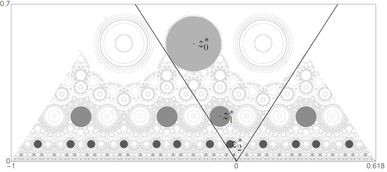
In this section we prove Theorems C and D. We begin by proving Theorem 7.1, which states that periodic points of a TCE are contained in periodically coded islands formed by unions of invariant circles.
We introduce reflective interval exchange transformations, relate them to TCEs and prove Theorem 7.4 which shows that for a family of TCEs for every such that belongs to a certain interval there is a horizontal periodic orbit for the TCE.
The final part of the section contains the proof of Theorems C and D.
We define the itinerary of a point , under , to be , with
for . Given , denote by , the circle of radius centered at . Let be the number of s in the -th first symbols of the itinerary of , for . In the next theorem we prove that for irrational, every periodic orbit that does not fall on the boundary of the partition must have a family of invariant manifolds. These are unions of circles centered on the periodic point parametrized by their radii.
Theorem 7.1.
Let be a periodic point of of period . Assume . There exists such that for all the union is an invariant set for . The orbit of any is dense on this set if and only if .
Proof.
We begin by showing that the itinerary of contains at least one symbol in . Assume by contradiction that is a periodic sequence of s and s. It is clear that
Since is a periodic point of of period we have . Therefore we get that , contradicting the assumption that is irrational.
Hence we can assume without loss of generality, since we can choose to start the periodic orbit at the first iterate that falls in for some . Since , then belongs to some open cell in the -th refinement of the partition. Since all points in this cell will share the first addresses in the itinerary, we have for . Therefore is such that
for some functions and . Since we have
From this it is easy to check that we can rewrite
and we get
| (7.1) |
This implies that is invariant in the largest circle with center contained in .
Take such that . We now see that for we have .
From (7.1) we have which implies that . Therefore . This implies that for all , we have , hence we also have for that . Therefore every has the same itinerary of . It follows that is also an invariant set for , since we can repeat the above argument for and conclude .
For any we know that if and only if for some . Since , we have . Therefore , since the reverse inclusion is clear. We can repeat this argument for and conclude that is an invariant set for . Therefore is an invariant set for .
Finally we prove that the orbit of any is dense on this set if and only if . Note that
We also have that acts as a rotation by an angle in , so the orbit of is dense if and only if . The statement for follows by . ∎
Recall the definition of interval exchange transformation (IET) in the Introduction. Given , , we say an IET is reflective if there is a point such that . Where denotes the norm of .
Recall, from the Introduction, that denotes the parameter region of all such that for some we have (1.6). The following lemma gives an alternative characterization of this set.
Lemma 7.2.
Let and . Then is reflective if and only if .
Proof.
Consider the map such that , for . By definition of this property, is reflective if and only if has a fixed point. Note that for all the restriction of to is an orientation reversing continuous bijection, hence has a fixed point if and only if there is a such that . It is simple to see that this condition is satisfied if and only if (1.6) holds. Thus is reflective if and only if as desired. ∎
Recall, from the Introduction, that given , is the set of all such that (1.6) holds, for some .
Given and set
| (7.2) |
We omit, for simplicity, the arguments of when this does not cause ambiguity.
Lemma 7.3.
Let , , and as in (7.2). We have and for all we have .
Proof.
We begin by showing that there is a and a such that
| (7.3) |
with as in (1.1). Since we have that is a reflective IET, hence there is a and a such that . Since , by taking we get (7.3). We show that for we have . By the definition of the map and by (1.2), for we have
| (7.4) |
In particular for , by the definition of , (7.3) and (7.4) we have
From (7.4) it follows that . We now prove that . By comparing the two identities above we get
Therefore, by (7.4) the slope of is equal to which coincides with . Thus , which completes the proof. ∎
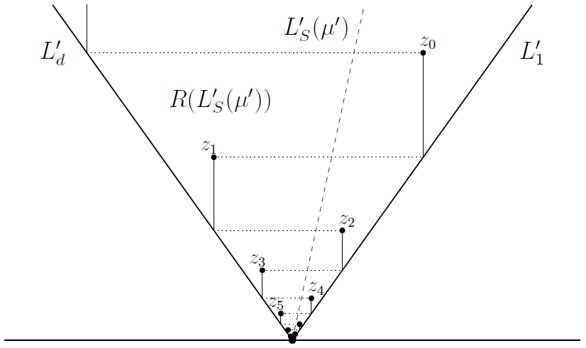
Given and such , let
Define the interval as
The following theorem shows that a simple condition for the existence of a horizontal periodic island, as defined in the Introduction, for a TCE. A visual depiction of this can be seen in Figure 3.
Theorem 7.4.
Let , , and as in (7.2). For every such that , has a horizontal periodic orbit at height , for a certain . If , then has an horizontal periodic island.
Proof.
Since and , by Lemma 7.3 we have for all that . Recall (6.1). We begin by proving that if for some we have , then . By the definition of and from (6.1) we have
From this, we have if and only if we have
By (4.2)
it is direct to see that these inequalities are satisfied if and only if .
We now prove that if , there is an satisfying
| (7.5) |
such that is a horizontal periodic orbit of at height .
We split the proof in two cases and , but omit the case as it is analogous to the other case.
Assume . As for , we have , moreover as we have and hence . Since this shows that
As and we have , hence by Theorem 5.2 we get that . As we get
By Theorem 5.2, is an affine map for and the map is also affine, in particular both maps are continuous for . Therefore by the two inequalities above, there must be a satisfying (7.5) such that
As , by Lemma 7.3 we have that
By Theorem 5.2, , hence by the two identities above we get that . Thus by the definition of , is a periodic orbit for .
Moreover by Lemma 2.1 we have that the imaginary part of remains constant, and equal to , throughout its orbit, hence it is an horizontal periodic orbit for .
Finally we show that if , then has a periodic island that contains this periodic orbit. Since and we can apply Theorem 7.1 which shows that this orbit shadows a periodic island which is formed by the union of infinitely many invariant circles. ∎
7.1. Proof of Theorem C
We divide the proof in two cases (resp. ) and prove that there is a non-empty open set (resp. ) such that for all (resp. ), has infinitely many horizontal periodic islands accumulating on the origin. Having proved this, taking gives the desired result.
We begin by considering the case . Given , consider the set
Since , we can take such that and take .
Let be as in (7.2). Consider the set of all , such that:
| (7.6) |
We now show that if , there is a such that for , we have (7.6).
Since the map is continuous for all and zero for , there is an , such that for all such that if:
| (7.7) |
then we have (7.6). By (7.2) we have
Using linearity of and simple trigonometric identities, from the above identity, we get
Since is independent of and we have , the map is continuous and therefore there is a such that for , we have (7.7) and thus (7.6).
We now show that there is a nonempty open set . To do this we construct an open set such that for we have . By (1.2) and (1.6), it suffices to show there is an such that we have
| (7.8) |
| (7.9) |
Since the above inequalities are strict, we have that there is a neighbourhood of , such that both inequalities are true for all .
We now prove there is satisfying (7.8) and (7.9). Assume first that and take such that and . Since , we have and , we have and , hence
thus (7.8) holds. We also have
hence, since , we get (7.9) as well.
Now assume and set , where
| (7.10) |
We show that (7.8) is true for . Since we have
By (7.10) we have , hence by the inequality above we have
which is equivalent to (7.8).
We now show that (7.9) is true for . Since for we have and we have
By (7.10) we have and hence by the inequality above we have that (7.9) is true for .
We now prove that for , has infinitely many horizontal periodic orbits accumulating on the origin. By Theorem 7.4 it suffices to show that for infinitely many we have . Note that we have
hence since we have
| (7.11) |
Assume first that , with . Using Hölder conjugacy of and it can be seen that (7.11) is equivalent to
By Theorem 4.3 (4.8), for all we have that , hence by the inequality above we get for infinitely many . Now assume . It can be seen that (7.11) is equivalent to:
By Theorem 4.3 (4.6), for all even we have that , hence by the inequality above we get for infinitely many .
We now show that there is a non-empty open set such that for all , has infinitely many horizontal periodic islands accumulating on the origin. By Theorem 7.4 it suffices to show that there is a non-empty open set such that for all we have .
Consider the sets
for . Note that we have if for some we have
By (7.2) and the two identities above it follows that we have if and only if for some .
Set . Since are codimension 1 closed subsets of , we have that is a non-empty open set and since for we have , has infinitely many horizontal periodic islands accumulating on the origin.
We now consider the case . This case is mostly analogous to the previous one, so for brevity we will only streamline the proof.
Given , consider the set
Take such that and take .
Consider the set , of all , such that:
By a similar argument to the previous case, if , there is a such that for , the expression above is satisfied.
To find a nonempty open set by (1.2) and (1.6), it suffices to show there is an such that we have (7.9) and:
Indeed it can be seen that both this inequality and (7.9) hold for the same choice of of the previous case.
We prove that for , has infinitely many horizontal periodic orbits accumulating on the origin. By Theorem 7.4 it suffices to show that for infinitely many we have . Note that we have
hence since we have
| (7.12) |
Assume first that . It can be seen that (7.12) is equivalent to
By Theorem 4.3 (4.7), for all odd we have that , hence by the inequality above we get for infinitely many . Now assume . It can be seen that (7.12) is equivalent to:
By Theorem 4.3 (4.9), for all we have that , hence by the inequality above we get for all .
Setting , we get that for we have , hence by Theorem 7.4 has infinitely many horizontal periodic islands at heights which converge to , hence accumulating on the real line.
7.2. Proof of Theorem D
Let be an invariant set for that contains a neighbourhood of the origin. By Theorem C it contains infinitely many periodic islands. Suppose there is a point with a dense orbit in . Then can get arbitrarily close to a periodic point , this implies that for some , is contained in a periodic island. Hence its orbit is contained in a circle thus contradicting the hypothesis that the orbit of is dense in .
References
- [1] Adler, R., Kitchens, B., Tresser, C. (2001). Dynamics of non-ergodic piecewise affine maps of the torus. Ergodic Theory and Dynamical Systems 21, 959-999.
- [2] Adler, R., Kitchens, B., Martens, M., Tresser, C., Wu, C.W., (2003). The mathematics of halftoning. IBM J. Res. Develop., 47, 5-15.
- [3] Alevy, I., Kenyon, R., Yi, R., (2018). A family of minimal and renormalizable rectangle exchange maps. arXiv:1803.06369
- [4] Ashwin, P., Chambers, W., Petrov, G., (1997). Lossless digital filter overflow oscillations; approximation of invariant fractals. Internat. J. Bifurcation Appl. Eng. 7 , no. 11, 2603–2610.
- [5] Ashwin, P. , Goetz, A. (2006). Polygonal invariant curves for a planar piecewise isometry. Trans. Amer. Math. Soc. 358 no. 1, 373-390.
- [6] Ashwin, P., Goetz, A. (2010). Cone exchange transformations and boundedness of orbits. Cambridge University Press, 30(5), 1311-1330.
- [7] Ashwin, P., Goetz, A., Peres, P. , Rodrigues, A. (2018). Embeddings of Interval Exchange Transformations in Planar Piecewise Isometries. arXiv:1805.00245.
- [8] Avila, A., Forni, G. (2007) Weak mixing for interval exchange transformations and translation flows, Ann. of Math. (2) , 165(2), 637-664.
- [9] Cornfeld, I. P. , Fomin, S. V., Sinai, Ya G. (1982) Ergodic Theory Grundlehren der Mathematisches Wissenschaften, 245, Springer-Verlag.
- [10] Davies, A. C., (1995). Nonlinear oscillations and chaos from digital filters overflow, Phil. Trans. Roy. Soc. A, 353, 85-99.
- [11] Deane, Jonathan H. B. (2006). Piecewise isometries: applications in engineering. Meccanica, 41, no. 3, 241-252.
- [12] Goetz, A. (2000). Dynamics of piecewise isometries. Illinois journal of mathematics, 44, 465 – 478, (2000).
- [13] Goetz, A., Dynamics of piecewise isometries. Thesis (Ph.D.) University of Illinois at Chicago. 1996.
- [14] Hooper, W. Patrick (2013) Renormalization of polygon exchange maps arising from corner percolation. Inventiones mathematicae, 191(2), 255-320.
- [15] Keane, M. S., (1975) Interval exchange transformations, Math. Z. 141, 25-31.
- [16] Kocarev, Lj. , Wu, C. W., Chua, L. O., (1996). IEEE Trans. Circuits Systems II, 43 , no. 3, 234246.
- [17] A. Ya. Khinchin, Continued Fractions. Translated from the third Russian edition (Moscow, 1961) by Scripta Technica. University of Chicago Press, Chicago, 1964. xii.
- [18] Lowenstein, John H., Vivaldi, Franco, Renormalization of a one-parameter family of piecewise isometries arXiv:1406.6910
- [19] Scott, A. J., (2003). Hamiltonian mappings and circle packing phase spaces: Numerical investigations. Phys. D, 181, 45-52.
- [20] Schwartz, R., (2007). Unbounded orbits for outer billiards. J. Modern Dynam. 3, 371 – 424.
- [21] Scott, A. J., Holmes, C.A., Milburn, G. (2001). Hamiltonian mappings and circle packing phase spaces. Phys. D, 155, 34-50.
- [22] Sturman, R., Meier, S., Ottino, J., Wiggins, S. (2008). Linked twist map formalism in two and three dimensions applied to mixing in tumbled granular flows. Journal of Fluid Mechanics, 602, 129-174.