Challenges to miniaturizing cold atom technology for deployable vacuum metrology

Abstract

Cold atoms are excellent metrological tools; they currently realize SI time and, soon, SI pressure in the ultra-high (UHV) and extreme high vacuum (XHV) regimes. The development of primary, vacuum metrology based on cold atoms currently falls under the purview of national metrology institutes. Under the emerging paradigm of the “quantum-SI”, these technologies become deployable (relatively easy-to-use sensors that integrate with other vacuum chambers), providing a primary realization of the pascal in the UHV and XHV for the end-user. Here, we discuss the challenges that this goal presents. We investigate, for two different modes of operation, the expected corrections to the ideal cold-atom vacuum gauge and estimate the associated uncertainties. Finally, we discuss the appropriate choice of sensor atom, the light Li atom rather than the heavier Rb.

1 Introduction

The emerging paradigm of the Quantum-SI focuses on building devices that obey three basic “laws”: (1) the sensor must be primary, (2) the sensor must report the correct quantity or no quantity at all, and (3) the uncertainties must be quantified and fit for purpose. Cold atoms represent a useful tool in developing Quantum-SI-based devices because they can be exquisitely manipulated and controlled. Deployable cold-atom sensors have the potential to revolutionize many types of Quantum-SI based measurements such as time, inertial navigation, and magnetometry. Here, we focus on the difficulties of miniaturization of cold-atom technologies for the purposes of vacuum metrology in the ultra-high vacuum (UHV, $p<10^{-6}$ Pa) to extreme high vacuum (XHV, $p<10^{-10}$ Pa) regimes.

A cold-atom vacuum gauge is based on the observation that the main source of atom loss from a cold-atom trap is collisions with background gas [1, 2, 3, 4, 5, 6, 7, 8, 9]. Because cold-atom traps tend to be shallow ($W/k_{B}\lesssim 1$ K, where $W$ is the trap depth and $k_{B}$ is Boltzmann’s constant) compared to room temperature, the vast majority of such collisions cause ejection of cold atoms from the trap. This random loss is well-characterized by an exponential decay of the trapped atom number with time. We are currently developing a laboratory-based cold-atom vacuum standard (CAVS) that will represent a primary standard for the pascal in the UHV and XHV ranges. This device will be capable of cooling and trapping different sensor atoms, including ⁶Li, ⁷Li, ⁸⁵Rb, and ⁸⁷Rb.

The dominant background gas in vacuum chambers operating in the UHV and XHV regimes is H₂. The determination of the loss rate coefficient for ⁶Li+H₂ is, in principle, a tractable calculation, and therefore establishes the primary nature of the CAVS. Extension to other background and process gases and to other sensor atoms will be accomplished by measurement of relative gas sensitivity coefficients (ratios of loss rate coefficients) [10].

The laboratory-scale CAVS currently in development at NIST is not deployable; it is neither portable, small, nor easy to use. It currently occupies an optical table with roughly 2 m² of area. A large experiment is required because of the large number of components needed to laser cool and trap atoms. First, atoms can only be trapped in UHV environments, generally requiring a large vacuum chamber with ion or getter pumps. Second, the workhorse of laser cooling, the three-dimensional magneto-optical trap (3D-MOT), requires optical access from six directions along three spatial axes. Third, generally good magnetic field stability is required, typically obtained by using large coils that cancel local magnetic fields and gradients. Shrinking the CAVS to something deployable thus represents an impressive challenge. Despite the difficulties, mobile cold atom systems have been constructed (e.g., an atom-based accelerometer [11]), and miniaturization continues to be an active area of research (for example, a proposal to construct a fully integrated chip-scale device [12]).

Presently, the most-widely-used gauge in the UHV and XHV regimes is the non-primary Bayard-Alpert ionization gauge [13, 14, 15], which requires $30$ cm³ and is controlled using a 2-U standard size rack-mountable controller. Thus, to make a deployable, cold-atom based gauge, we tailor our design to occupy a similar vacuum footprint.

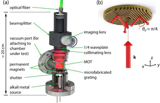
Figure 1: (a) Concept of the p-CAVS, a cold atom-based vacuum sensor that has the same vacuum footprint as a typical ion or extractor gauge. (b) Geometry of our grating MOT. A single laser beam (large, red arrow) traveling along $\hat{z}$ is diffracted into six different beams (small, red arrows) by three reflective, gold diffraction gratings whose lines form superimposed triangles and diffract light at $\theta_{d}=\pi/4$ with respect to the normal of the grating ($-\hat{z}$). The lines of the diffraction grating are not to scale.

Our current design for a portable CAVS (herein referred to as p-CAVS), shown in Fig. 1, is under active development. Currently, many of its individual components are being tested separately, and, as such, the final design is still in flux. At its core, it uses a micro-fabricated diffraction grating that generates the necessary spatial beams for laser cooling and trapping [16, 17]. This planar MOT is a variant of previously developed non-planar MOTs like tetrahedral [18] and pyramidal MOTs [19]. The p-CAVS can create both a magneto-optical trap and a quadrupole magnetic trap, yielding two possible modes of operation. In this paper, we focus on the physical principles for its operation and the associated uncertainties (Sec. 2). Secondly, we describe some of the technical design features and their motivation. These choices depend on the requirements for a deployable vacuum gauge, including how it will be used and treated in the field (Sec. 3). We conclude by motivating our choice of atomic species (Sec. 4). We include a short appendix describing the atomic physics used within this paper. Throughout the paper, we focus primarily on type-B uncertainties and assume $k=1$. Type-A uncertainties are briefly discussed in Sec. 2.3.

2 Principle of operation and associated uncertainties

The number of cold atoms $N(t)$ in a trap decays exponentially due to collisions with background gas molecules, i.e. $N(t)=N_{0}e^{-\Gamma t}$, where $\Gamma=n\langle K\rangle$ is the loss rate, $K=v\sigma$ is the loss rate coefficient, $n$ is the number density of the background gas, $\sigma(E)$ is the total cross section for a relative collision energy $E=\mu v^{2}/2$ and relative velocity $v$. Here, $\mu$ is the reduced mass, $N_{0}$ is the initial number of trapped cold atoms, and $\langle\cdots\rangle$ represents thermal averaging. In the XHV and UHV regimes, the ideal gas law is an excellent equation of state of the background gas, and thus we can relate the loss rate to the pressure through

$$p=\frac{\Gamma}{\left<K\right>}k_{B}T,$$ (1)

where $T$ is the temperature of the background gas. Equation 1 represents the ideal operation of the CAVS and p-CAVS.

Perhaps the most crucial quantity in Eq. 1 is $\left<K\right>$. We described the techniques for determining this quantity in a previous work [10]. We intend to calculate a priori the collision cross section for ⁶Li+H₂. For other gases, we plan to measure the ratio of loss rate coefficients to that of ⁶Li+H₂. In the present work, we will assume the uncertainty in $\left<K\right>$ to be $5$ %, an estimate based on the expected results of a laboratory-scale CAVS. Both theoretical scattering calculations and experimental work are ongoing.

	Li (2S)	Li∗ (2P)	Rb (5S)	Rb∗ (5P)
H2 [20]	83		160
He [21, 22]	23		45
H2O	150	100	280	280
N2	180	130	350	350
O2	160	120	310	310
Ar [21, 22]	180		340
CO2	270	190	520	510

Table 1: Estimated $C_{6}$ coefficients in atomic units. Entries without references were calculated using the Casimir-Polder integral, for which we estimate a 10 % uncertainty for the values. The coefficients do not depend on isotope to the accuracy given.

Ab initio quantum-mechanical scattering calculations are difficult, but we can estimate the cross section using semiclassical theory [23, 24] for a cold, sensor atom of mass $m_{c}$ and a (relatively-hot) room-temperature background-gas atom or molecule of mass $m_{h}$. In this theory, the isotropic, long-range attractive part of the inter-molecular potential fully determines the total elastic cross section. This part of the potential is dominated by a van der Waals interaction $-C_{6}/r^{6}$, where $C_{6}$ is the dispersion coefficient and $r$ is the separation between the cold atom and the background gas molecule. Table 1 lists $C_{6}$ for various combinations of cold atoms (both ground S and first excited P states) and background gases as calculated using the Casimir-Polder relationship,

$$C_{6}=\frac{3}{\pi}\int_{0}^{\infty}\alpha_{A}(i\omega)\alpha_{B}(i\omega)\ d\omega$$ (2)

for species $A$ and $B$. Accurate dynamic polarizabilities $\alpha(\omega)$ as a function of frequency $\omega$ exist for each alkali atoms’ ground state [25]. The dynamic polarizability of the excited state has been calculated for Li (2P_3/2) [26] and can be inferred from transition frequencies and matrix elements for Rb (5P_3/2) [27]. For common background gases, we use dynamic polarizabilities found in the literature for water [28], nitrogen [29], oxygen [30], and carbon dioxide [30]. For Li, the dispersion coefficient is a factor of two smaller than Rb for the same background molecule. Coincidentally, there appears to be little to no difference in the $C_{6}$ coefficients for the 2P and 2S states of Rb.

Within the semiclassical theory [23, 24], we calculate both the differential and total cross sections from the semiclassical phase shift for partial wave $\ell$,

$$\eta_{\ell}(E)=\frac{32\pi}{3}\frac{(E/E_{6})^{2}}{\ell^{5}},$$ (3)

where $E_{6}=\hbar^{2}/(2\mu x_{6}^{2})$ is the van der Waals energy, $x_{6}=(2\mu C_{6}/\hbar^{2})^{1/4}$ is the van der Waals length, and $\hbar$ is the reduced Planck constant [24]. This leads to a total elastic cross section $\sigma(E)=\sigma_{0}(E/E_{6})^{3/10}x_{6}^{2}$, where $\sigma_{0}=5/2\cdot 3^{2/5}(1+\sqrt{5})\pi^{7/5}\Gamma(3/5)/(10\cdot 2^{3/5})=6.125\cdots$. We thermally average the loss rate coefficient by assuming that the cold atoms (typically with temperatures $\lesssim 1$ mK) are stationary relative to the room temperature gas. The result is

$$\langle K\rangle = \frac{1}{\mathcal{Z}}\int d^{3}p_{h}e^{-p_{h}^{2}/(2m_{h}k_{B}T)}K(E)$$ (4)

$$= \kappa\left(\frac{\mu}{m_{h}}\frac{k_{B}T}{E_{6}}\right)^{3/10}x_{6}^{3}\frac{E_{6}}{\hbar}\propto\frac{(k_{B}T)^{3/10}}{m_{h}^{3/10}}C_{6}^{2/5},$$ (5)

where $\mathbf{p}_{h}$ is the initial momentum of the background gas molecule, $E=(m_{c}/M)[p_{h}^{2}/(2m_{h})]$, $M=m_{c}+m_{h}$, $\kappa=4\Gamma(9/5)\sigma_{0}/\sqrt{\pi}=12.88\cdots$, and $\mathcal{Z}$ is the partition function for the background gas. In general, $E_{6}/k_{B}\approx 1$ mK and $k_{B}T/E_{6}\gg 1$. The last proportionality shows the dependence on $C_{6}$, $m_{h}$, and $T$; surprisingly, it does not depend on $m_{c}$.

The largest correction to Eq. 1 is the lack of a one-to-one correspondence between a collision and the ejection of a cold atom from its trap [31, 32]. To eject an atom, the final kinetic energy of the initially cold atom must be at least $W$, the depth of a trap that is equally deep in any direction. Atoms are not ejected for scattering angles $\theta_{r}$ less than the critical angle $\theta_{c}$, defined by

$$\cos\theta_{c}=1-\frac{1}{2}\frac{m_{c}}{\mu}\frac{W}{E},$$ (6)

as follows from energy and momentum conservation assuming a cold atom initially at rest. The loss rate coefficient for such glancing collisions with an isotropic potential is

$$K_{\rm gl}(W,E)=2\pi\int_{0}^{\theta_{c}(W)}v\frac{d\sigma(E,\theta_{r})}{d\Omega_{r}}\ \sin\theta_{r}d\theta_{r},$$ (7)

where $d\sigma/d\Omega_{r}$ is the differential cross section, where $\theta_{c}(W)$ is given by Eq. 6. In the semiclassical theory, the thermally-averaged result to first order in trap depth $W$ is

$$\langle K_{\rm gl}(W)\rangle = \frac{1}{\mathcal{Z}}\int d^{3}p_{h}e^{-p_{h}^{2}/(2m_{h}k_{B}T)}K_{\rm gl}(W,E)$$ (8)

$$\approx \kappa\zeta\frac{m_{c}}{\mu}\frac{W}{E_{6}}\left(\frac{\mu}{m_{h}}\frac{k_{B}T}{E_{6}}\right)^{-1/10}x_{6}^{3}\frac{E_{6}}{\hbar},$$ (9)

where $\zeta=25\pi^{13/10}[\Gamma(8/5)]^{3}/(4\cdot 6^{6/5}\sigma_{0})=0.3755\cdots$. We find the higher order corrections numerically by integrating

$$\frac{d\sigma}{d\Omega_{r}}=\left|\frac{1}{2i(E/E_{6})^{1/2}}\sum_{\ell=0}^{\infty}(2\ell+1)P_{\ell}(\cos\theta_{r})\left(e^{2i\eta_{\ell}(E)}-1\right)\right|^{2}x_{6}^{2},$$ (10)

where $P_{\ell}(x)$ are the Legendre polynomials and $\eta_{\ell}(E)$ is given by Eq. 3.

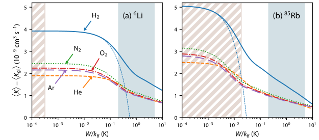
Figure 2: (Color online) Glancing-collision-corrected loss rate coefficient for ground-state ⁶Li(²S), panel (a), and ⁸⁵Rb(²S), panel (b), as a function of trap depth for various background gases at $T=293$ K. For H₂, the thin-dashed curve shows the first-order result in $W$, Eq. 7. The red-striped (blue) shaded regions highlight the accessible range of trap depths with a magnetic (magneto-optical) trap. Note that for magnetic trapping, we assume that cold atoms are in the $F=I-1/2$ hyperfine state, which leads to different maximum trap depths for Li and Rb.

These glancing collisions change the ideal CAVS operation (Eq. 1) to

$$p=\frac{\Gamma}{\left<K\right>-\left<K_{\rm gl}(W)\right>}k_{B}T.$$ (11)

Figure 2 shows the CAVS loss rate coefficient with glancing collisions, $\left<K\right>-\left<K_{\rm gl}(W)\right>$, for several cold atomic species and room-temperature background gases as a function of trap depth based on the numerical integration of Eq. 10. This plot has several interesting features. First, for the same background gas, Rb, with its larger van-der-Waals coefficients, has a larger loss rate coefficient than Li. Second, $\langle K\rangle$ for H₂ collisions is twice as large as for other gases, due primarily to its smaller mass. Third, the first order behavior, Eq. 7, is an excellent approximation until $[\langle K\rangle-\langle K_{\rm gl}(W)\rangle]/\langle K\rangle\approx 0.9$. At this point, the linear behavior starts to give way to a logarithmic dependence on $W$. This appears as a straight line on the log-linear scale. In fact, $\langle K_{\rm gl}(W)\rangle/\langle K\rangle\approx 0.1$ defines a crossover trap depth, $W_{c}$, which scales as

$$W_{c}\propto\frac{m_{h}^{1/10}}{m_{c}^{1/2}(m_{c}+m_{h})^{1/2}}\frac{1}{C_{6}^{3/10}}.$$ (12)

Thus, for the same background gas, Rb, which is both more massive than Li and has larger $C_{6}$ coefficients, has a smaller $W_{c}$. As shown in Fig. 2, the transition in the $\langle K\rangle-\langle K_{\rm gl}(W)\rangle$ behavior occurs at higher $W$ for Li ($W_{c}/k_{B}\approx 0.5$ K) compared to Rb ($W_{c}/k_{B}\approx 20$ mK).

There are two traps that are easy to realize in the p-CAVS given our design constraints: a MOT and a quadrupole magnetic trap. Each has a different trap depth and, consequently, different fractions of glancing collisions. MOTs generally have depths ranging from 200 mK to 5 K depending on their parameters, as shown in Fig. 2, where glancing collisions reduce the losses by over one-half. Quadrupole magnetic traps have depths of the order of 100 mK or lower, determined by the atomic state. As a result, the uncertainty budgets associated with operating these two types of traps are different.

The determination of $\Gamma$ from atoms contained within the traps is also different. In a MOT, the measurement proceeds by loading the trap and observing the loss of atoms from the trap by continuously monitoring their fluorescence. Thus, making a single MOT yields many points on the $N(t)$ curve. This is in contrast to operation with a quadrupole magnetic trap, which first requires loading atoms into a MOT followed by optical pumping into the magnetically-trapped atomic state. After free evolution, the atoms in the magnetic trap are recaptured into the MOT and counted by measuring the fluorescence. In this operation, a single load of the magnetic trap yields a single point on the $N(t)$ curve. Constructing a decay curve with a reasonable signal to noise thus requires loading and measuring multiple times. Thus, this mode of operation is significantly slower than that of the MOT; however, as we shall see, it is more accurate.

2.1 Fast operation of p-CAVS: magneto-optical trap

Operating the MOT as a pressure sensor presents several type-B (systematic) uncertainties, some of which were anticipated in Ref. [5]. Glancing collisions are the dominant correction to the ideal CAVS operation in a MOT. Translating the loss rate of atoms from the MOT into a pressure therefore requires knowledge of its trap depth. Two trap-depth-measurement techniques have been employed: inducing two-body loss with a known, final kinetic energy with a catalyst laser [33] and comparing the background-gas induced MOT loss rates to a magnetic trap with known depth [34]. These two methods have been shown to yield identical results [34]. Given their complexity, however, it is not clear whether such measurements could be implemented in a sensor.

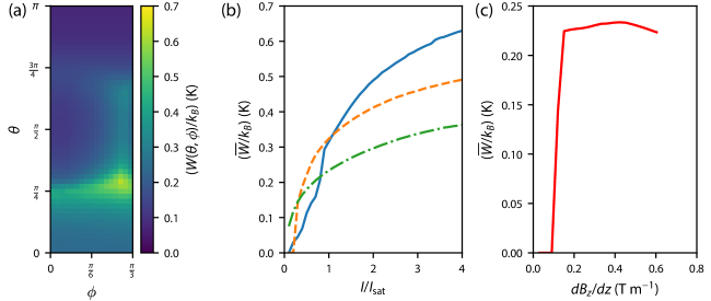
Figure 3: Trap depth $W$ for a typical, three beam grating MOT for Li. (a) Angularly-resolved $W(\theta,\phi)$ for an incident beam with $I/I_{\rm sat}=1$, $\Delta/\gamma=-1$, and $dB_{z}/dz=0.5$ T m^-1. (b) Average trap depth as a function of incident beam intensity for detunings $\Delta/\gamma=-3.0$ (solid blue), $-2.0$ (dashed orange), and $-1.0$ (dashed-dot green) with $dB_{z}/dz=0.5$ T m^-1. (c) Average trap depth as a function of magnetic field gradient for $I/I_{\rm sat}=1$ and $\Delta/\gamma=-1$.

Models of the trap depth of a MOT have been developed and find quantitative agreement with measurements of two-body collisions between cold atoms [35]. The models assume an atom with an optical cycling transition between a ground state with electronic orbital angular momentum $L=0$ (S) and an excited state with $L=1$ (P). (Here, we ignore effects due to spin-orbit coupling and hyperfine structure.) The non-conservative force on an atom in a MOT results from the interplay of a spatially-varying magnetic field $\mathbf{B}(\mathbf{r})$ and multiple laser beams $i$ with the same frequency detuning $\Delta$ with respect to the atomic transition but different wavevectors $\mathbf{k}_{i}$ and circular polarizations $\epsilon_{i}=\pm 1$. The resulting force on the atom with position $\mathbf{r}$ and velocity $\mathbf{v}$ is

$$\mathbf{F}(\mathbf{r},\mathbf{v}) = \sum_{i}\sum_{m=-1}^{1}P_{i}(m)$$ (13)

$$\times\frac{\hbar\mathbf{k}_{i}\Gamma}{2}\frac{s_{i}}{1+\sum_{j}s_{j}+4[\Delta-\mathbf{k}_{i}\cdot\mathbf{v}-(m\mu_{B}|\mathbf{B}(\mathbf{r})|/\hbar)]^{2}/\gamma^{2}},$$

where $s_{i}=I_{i}/I_{\rm sat}$ is the saturation parameter of beam $i$ with intensity $I_{i}$. Here, the saturation intensity $I_{\rm sat}$ and linewidth $\gamma$ are properties of the atom and $\mu_{B}$ is the Bohr magneton. The probability of making a transition to an excited angular momentum projection $m$ is

$$P_{i}(m)=|d^{1}_{\epsilon_{i}m}(\pi/2-\xi_{i})|^{2}=\left\{\begin{array}[]{ll}\left(1-\epsilon_{i}\sin\xi_{i}\right)^{2}/4,&m=\pm 1\\ (\cos^{2}\xi_{i})/2,&m=0\end{array}\right.,$$ (14)

where $\xi_{i}$ is the angle between $\mathbf{k}_{i}$ and $\mathbf{B}(\mathbf{r})$ and $d^{j}_{mm^{\prime}}(\theta)$ is a Wigner rotation matrix.

We model the MOT trap depth for the p-CAVS using Eqs. 13–14 with the beam geometries, polarizations, and magnetic field specific for our device as shown in Fig. 1b. We use the magnetic field gradient

$$\mathbf{B}(\mathbf{r})=\frac{dB_{z}}{dz}\left[z\hat{z}-\frac{1}{2}\rho\hat{\rho}\right]$$ (15)

in cylindrical coordinates $\mathbf{r}=(\rho,\phi,z)$ with parameter $dB_{z}/dz$. The magnetic field is zero at $\mathbf{r}=0$. The diffraction grating shown is positioned at $z_{g}=+5$ mm and is illuminated with a $\epsilon=+1$ polarized Gaussian beam traveling along the $+\hat{z}$ direction. The beam’s $1/e^{2}$ radius is 15 mm. The diffraction grating lines are made from superimposed equilateral triangles. The triangles continue outwards until clipped by a circle with diameter 22 mm. A central, triangle-shaped through-hole, fitting an inscribed circle of radius 2.5 mm, produces a vacuum connection to the rest of the chamber. The three sides of the triangles form three grating sections that each produce two beams with angle $\theta_{d}=\pi/4$ with respect to the normal of the grating ($-\hat{z}$), one points toward the central axis of the MOT and the other outwards. Only the inward beams contribute to forming the MOT. The polarizations of these reflected beams is $\sigma^{-}$; their intensity profile is assumed to be the same as the incident beam, but clipped according to the area of the grating section and translated along its $\mathbf{k}_{i}$ vector. The grating produces no zero-order reflection and equal $\pm 1$ diffraction orders with efficiency $\eta=1/3$ and absorbs $1/3$ of the incident intensity. The resulting ratio of the reflected beam intensity to that of the incident is $\eta/\cos\theta_{d}$, where the cosine describes the decrease in the beam’s cross section.

The magnetic field zero does not specify the center of the trap for a grating MOT. Unlike a standard 3D-MOT [36] where $P_{i}(m=0)=0$ along $\rho=0$, $P_{i}(m=0)$ is larger than $P_{i}(m=\pm 1)$ for the beams reflected from the grating, producing a position-independent force from these beams [37]. We find the trap center $\mathbf{r}_{0}=(0,0,z_{0})$ by placing an atom at rest at $\mathbf{r}=0$, integrating the equations of motion (including the shape of the beams) and following its damped motion to the center. For alkali-metal atoms, MOTs are either overdamped or slightly underdamped. For our parameters, $z_{0}>0$.

The temperature of the cold-atom cloud is small compared to the trap depth; therefore, the atoms are initially concentrated near the center of the trap. After a collision with a background particle, they acquire momentum $\mathbf{q}_{c}$ directed at azimuthal angle $\phi$ and polar angle $\theta$ in the laboratory frame. To determine the trap depth $W$, we can numerically integrate the equations of motion starting from the center of the trap. For each pair of ($\theta,\phi$), the trap depth $W(\theta,\phi)$ is given by the initial kinetic energy $q_{e}^{2}/(2m_{c})$, where $v_{e}=q_{e}/m_{c}$ is the escape velocity.

Figure 3a shows $W(\theta,\phi)$ for a Li grating MOT with $\Delta/\gamma=-1$, $dB_{z}/dz=0.5$ T m^-1, and the saturation parameter $s=1$ for the incident beam. We observe significant anisotropy in the trap depth, varying from 0.1 K to 0.7 K (only azimuthal angles of $0<\phi<\pi/3$ are shown because of the three-fold symmetry of the grating MOT). This is possible because MOTs are overdamped: an atom launched from the center of the trap with $q_{c}<q_{e}$ does not move chaotically through the trap, but instead quickly returns to the center. The polar angle at which the trap depth is largest is $\theta=\pi/4$, corresponding an atom moving directly into the reflected beams. The azimuthal angle that maximizes the depth is $\phi=\pi/3$, where two reflected beams both apply equal force. Finally, the shallowest direction corresponds to $\theta=\pi$, or into the incoming laser beam.

The anisotropy of $W(\theta,\phi)$ complicates the calculation of $\langle K_{\rm gl}(W)\rangle$. The thermally averaged loss coefficient in this case becomes

$$\overline{\langle K_{\rm gl}(W)\rangle}=\frac{1}{\mathcal{Z}}\int d^{3}p_{h}e^{-p_{h}^{2}/(2m_{h}k_{B}T)}\int d\Omega_{r}\ v\frac{d\sigma}{d\Omega_{r}}\ H\left(W(\theta,\phi)-\frac{q_{c}^{2}}{2m_{c}}\right),$$ (16)

where $H(x)$ is the Heaviside step function, $d\Omega_{r}=\sin\theta_{r}d\theta_{r}d\phi_{r}$, and $\theta_{r}$ and $\phi_{r}$ are the scattering angles. Realizing that the angle between the initial $\mathbf{p}_{h}$ and final $\mathbf{q}_{c}$ is uniquely determined by $\theta_{r}$, we interchange variables and find

$$\overline{\langle K_{\rm gl}(W)\rangle}=\frac{1}{4\pi}\int d\Omega\ \langle K_{\rm gl}(W(\theta,\phi))\rangle,$$ (17)

where $d\Omega=\sin\theta d\theta d\phi$. We compute an angle dependent $\overline{\langle K_{\rm gl}(W)\rangle}$ using $W(\theta,\phi)$ and Eq. 10 for each $(\theta,\phi)$ and average over all angles. For the present work, we use the approximation $\overline{\langle K_{\rm gl}(W)\rangle}\approx\langle K_{\rm gl}(\overline{W(\theta,\phi)})\rangle$, where $\overline{W}=\int d\Omega\ W(\theta,\phi)/(4\pi)$, which is accurate within the currently known MOT uncertainties (see below).

We have studied the angularly-averaged trap depth $\overline{W}$ for a Li grating MOT to investigate the dependence on detuning $\Delta$, intensity of the incident beam $I$, and magnetic field gradient. The results are shown in Fig. 3. As with a standard six-beam MOT, the trap depth increases with increasing $s$ for a given $|\Delta/\gamma|$, shown in Fig. 3b. For small $s$, the large $P_{i}(m=0)$ component of the reflected beams creates a complicated dependence on $|\Delta/\gamma|$. It also causes a sudden breakdown of the trap for magnetic field gradients $<0.1$ T m^-1, shown in Fig. 3c. This “critical” magnetic field gradient is the gradient required to balance the force toward the grating from the magnetic-field sensitive $m=+1$ component with the force away from the grating from the magnetic-field insensitive $m=0$ component.

The uncertainty in the pressure due to uncertainty in the MOT’s trap depth is suppressed. In particular, the fractional uncertainty in the measured pressure is $\delta p/p=\delta\overline{W}/\overline{W}\log(\overline{W}/W_{0})|$, based on Eq. 11 and $\langle K\rangle-\langle K_{\rm gl}(\overline{W})\rangle\propto-A\log(\overline{W}/W_{0})$ for MOTs, where $A$ and $W_{0}$ are constants that depend on the background gas and sensor atom. For Rb, $W_{0}/k_{B}\approx 300$ K for most collisions other than H₂; for Li, $W_{0}\approx 1000$ K for collisions other than H₂. For example, consider an uncertainty $\delta\overline{W}/\overline{W}\approx 20$ % and $\overline{W}/k_{B}\approx 1$ K; here, $\delta p/p\approx 8$ % for Rb and $7$ % for Li. The actual uncertainty $\delta\overline{W}$ is currently difficult to establish. We have tested our model against the published data in Ref. [34], and find agreement to within the experimental error bars for the smallest trap depths. Based on this comparison, we currently estimate the fractional uncertainty $\delta\overline{W}/\overline{W}$ of the order of tens of per cent. It is our intent to further improve the accuracy and uncertainty of these models.

The second correction to the measured pressure by a MOT comes from the fact that a non-negligible fraction of atoms are in the excited P state, which has different $C_{6}$ coefficients compared to the ground S state (see Tab. 1). With this correction, Eq. 11 becomes

$$p=\frac{\Gamma}{(1-P_{\rm ex})\left<K-K_{\rm gl}(W)\right>_{\rm ground}+P_{\rm ex}\left<K-K_{\rm gl}(W)\right>_{\rm excited}}k_{B}T,$$ (18)

where $P_{\rm ex}$ is the probability of an atom to be in the excited state. For grating MOTs, $\mu_{B}|B(\mathbf{r}_{0})|/\hbar\ll\Delta$, and

$$P_{\rm ex}=\frac{1}{2}\sum_{i}\frac{s_{i}}{1+\sum_{j}s_{j}+4(\Delta/\gamma)^{2}}\ .$$ (19)

Typically, $s_{i}\approx 1$ and $\Delta/\gamma\approx-1$, making $P_{\rm ex}\approx 25$ %. The uncertainty in $P_{\rm ex}$ is dominated by that of $s_{j}$, which at best has $\delta s_{j}/s_{j}\approx 5$ %, leading to $\delta P_{\rm ex}/P_{\rm ex}\approx 12$ %. From our numerical results, $\left<K-K_{\rm gl}(W)\right>\propto(C_{6})^{0.35}$ in the MOT regime, and $\left<K-K_{\rm gl}(W)\right>_{\rm excited}/\left<K-K_{\rm gl}(W)\right>_{\rm ground}\approx(C_{6,{\rm P}}/C_{\rm 6,{\rm S}})^{0.35}$. We estimate an uncertainty in the ratio of 14 % based on our uncertainty in $C_{6}$. For a typical MOT, the fractional uncertainty in the measured pressure is relatively small: $3$ % for both Li and Rb. Note that in this analysis we neglect the possibility of inelastic collisions with atoms in the excited state, which change the internal state of the cold atom. These effects will need to be further studied.

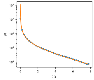
Figure 4: Number of ⁷Li atoms as a function of time, blue points, in a standard six-beam MOT showing light-assisted two-body loss at early times ($t<1$ s) and exponential decay at longer times ($t>2$ s). The orange curve shows a fit to Eq. 20. The statistical uncertainty in the data is comparable to the size of the points.

Finally, another complication with using a MOT to measure pressure is the presence of light-assisted collisions between cold atoms [38, 39, 40, 41]. With these collisions, the number of atoms in the trap $N$ obey

$$\frac{dN}{dt}=-\Gamma N-K_{2}N^{2}-K_{3}N^{3}-\cdots,$$ (20)

where $K_{n}$ is an $n$-body loss parameter that depends on the intensity and detuning of the MOT light. Figure 4 shows such a decay curve with large two-body loss measured in a standard, six-beam MOT of ⁷Li atoms. The curvature observed at early times indicates the presence of two-body collisions. One can fit the data to Eq. 20 to accurately separate $n$-body loss from the exponential loss due to background gas collisions. No evidence of three- or higher-body loss was found in the data in Fig. 4. For these data, the MOT light is red-detuned to the $F=2\rightarrow F^{\prime}=3$ transition with $\Delta/\gamma=-2.0(1)$ and $dB/dz\approx 0.5$ T/m. Each of the six Gaussian beams has an intensity of 7.4(4) mW/cm² with a $1/e^{2}$ diameter of 1.42(7) cm. Repump light is provided by the $+1$ sideband of an electro-optic-modulator operating at 813 MHz. Apporoximately 55 % of the power remains in the carrier (red detuned with respect to $F=2\rightarrow F^{\prime}=3$) and $\approx 22$ % of the power is in the repump (tuned to resonance with the $F=1\rightarrow F^{\prime}=2$ transition).

2.2 Accurate operation: Quadrupole magnetic trap

Unlike MOTs, magnetic traps are conservative traps: an atom’s kinetic energy must decrease by the same amount as its internal energy increases. In free space, Maxwell’s equations only allow minima in $|\mathbf{B}(\mathbf{r})|$ (Earnshaw’s theorem). Therefore, only states whose internal energy $\mathcal{E}$ increases with $|\mathbf{B}(\mathbf{r})|$, i.e. $d\mathcal{E}/dB>0$, can be trapped. In this section, we consider the quadrupole trap generated by the MOT magnetic field given by Eq. 15. This trap has its center at $\mathbf{r}=0\neq\mathbf{r}_{0}$.

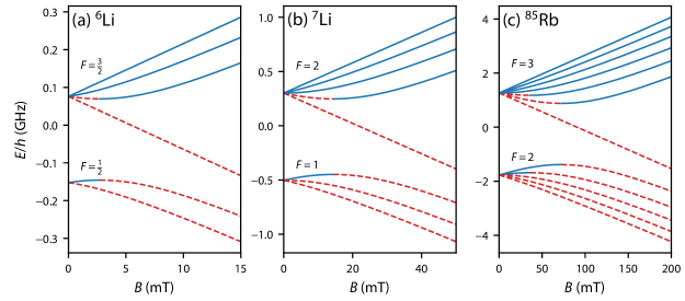
Figure 5: Energy of the magnetic sublevels as a function of magnetic field for (a) ⁶Li, (b) ⁷Li, and (c) ⁸⁵Rb. Blue, solid curves (red, dashed) correspond to states that are (are not) magnetically trappable. Note the different scales.

The energy of the internal states of ⁶Li(²S), ⁷Li(²S), and ⁸⁵Rb(²S) are shown in Fig. 5. Here, we include the hyperfine and Zeeman interactions. The former gives rise to two non-degenerate states at $\mathbf{B}=0$, denoted by $F=I\pm 1/2$, where $I$ is the nuclear spin. For ⁶Li, ⁷Li, and ⁸⁵Rb, $I=1$, $3/2$, and $5/2$ respectively. For non-zero $B$, the levels split according to projection $m_{F}=-F,-F+1,\cdots,F$.

Magnetic traps in the limit $B\rightarrow\infty$ have infinite trap depth for states with $F=I+1/2$ for these three atoms. Hence, these states are impractical for CAVS operation. Instead, we focus on the state $\left|F=I-1/2,m_{F}=-(I-1/2)\right>$, which has an energy

$$\mathcal{E}=-\frac{\Delta_{\rm HF}}{2(2I+1)}+g_{I}m_{F}\mu_{B}B-\frac{\Delta_{\rm HF}}{2}\left[1+\frac{4}{2I+1}\frac{gm_{F}\mu_{B}B}{\Delta_{\rm HF}}+\left(\frac{g\mu_{B}B}{\Delta_{\rm HF}}\right)^{2}\right]^{1/2}$$ (21)

where $g=g_{I}-g_{J}$, $g_{I}$ and $g_{J}$ are the nuclear and electronic gyromagnetic ratio respectively, and $\Delta_{\rm HF}$ is the zero-field energy splitting. This state has a maximum energy at a finite $B_{\rm max}$ and trap depth $W_{\rm max}=E(B_{\rm max})-E(B=0)$. Neglecting the $g_{I}m_{F}\mu_{B}B$ term in Eq. 21 yields

$$B_{\rm max}\approx\frac{2I-1}{2I+1}\frac{\Delta_{\rm HF}}{g\mu_{B}}$$ (22)

and

$$W_{\rm max}\approx\Delta_{\rm HF}\left(\frac{1}{2}-\sqrt{\frac{2I-1}{2(2I+1)^{2}}}\right).$$ (23)

Table 2 lists $B_{\rm max}$ and $W_{\rm max}$ for Li and Rb isotopes. The uncertainty $B_{\rm max}$ and $W_{\rm max}$ is set by the uncertainty in the atomic physics parameters, which are known to better than 1 ppm.

Species	$B_{\rm max}$ (mT)	$W_{\rm max}/k_{B}$ (mK)	$dB_{z}/dz$ (T m-1)	$z_{T}$ (mm)
6Li	2.7168	0.31409	0.50	5
7Li	14.357	2.5946	0.50	30
85Rb	72.251	18.578	0.15	480
87Rb	244.30	62.971	0.15	1600

Table 2: Energy-maximizing magnetic fields $B_{\rm max}$, resulting trap depths $W_{\rm max}$, typical magnetic field gradients used in a magneto-optical trap $dB_{z}/dz$, and resulting trap size $z_{T}=B_{\rm max}/(dB_{z}/dz)$ for various species. Note that $B_{\rm max}$ and $W_{\rm max}$ are typically known to within a ppm, while $dB_{z}/dz$ and $z_{T}$ are estimates.

Using the $dB_{z}/dz$ for a MOT sets the characteristic size of the magnetic trap through $z_{T}=B_{\rm max}/(dB_{z}/dz)$. Table 2 lists both $dB_{z}/dz$ and $z_{T}$. The size of initial cold atom does not equal $z_{T}$, but is set by its temperature out of the MOT, $\lesssim 1$ mK. One then expects from the virial theorem a cloud size $z_{c}\approx 5$ mm for Li and $z_{c}\approx 20$ mm for Rb. For ⁶Li, with $z_{c}>z_{T}$, this causes some loss of atoms when transferred from the MOT to the magnetic trap. For Rb, with $z_{c}>z_{g}$, the cloud will expand into the grating, which is the closest in-vacuum component. This may require increasing the magnetic field gradient to reduce the size of the initial cold-atom cloud.

The grating decreases the trap depth when $z_{T}>z_{g}$, as higher-energy atoms eventually collide with and, most likely, stick to the grating. (The classical orbits in a quadrupole trap are not closed.) The trap depth is then determined by geometry, i.e., $W=|gm_{F}\mu_{B}(dB_{z}/dz)z_{g}|$; its fractional uncertainty is set by $\delta z_{g}/z_{g}$ and $\delta(dB_{z}/dz)/(dB_{z}/dz)$. For Rb with $z_{g}=5(1)$ mm and $dB_{z}/dz=0.15(2)$ T m^-1, $W=1$ mK and $\delta W/W\approx 25$ %. In a magnetic trap, Eq. 8 is an excellent approximation and thus the fractional uncertainty in the glancing collision fraction is also 25 %.

Glancing collisions in a magnetic trap can still lead to loss of atoms from the trap. The average energy deposited by a glancing collision is $Q=W/2$. Moreover, the average amount of energy necessary to cause ejection is $\approx W-k_{B}T_{c}$, where $T_{c}$ is the temperature of the cold atoms. Consequently, starting in the limit where $k_{B}T_{c}\ll W$, glancing collisions only heat the gas and the loss rate is given by $\Gamma=n(\langle K\rangle-\langle K_{\rm gl}(W)\rangle)$. As the trapped gas warms and $k_{B}T_{c}\gtrsim W/2$, more of the glancing collisions start contributing to the loss and $\Gamma$ approaches $n\langle K\rangle$. Because $\Gamma$ depends on $T_{c}$ and time, we expect that this will cause non-exponential decay and thus may be separable in a manner similar to the $n$-body loss of Eq. 20. This heating through glancing collisions is a problem that we also anticipate with the laboratory-scale CAVS and are currently performing Monte-Carlo studies to understand. For the present analysis, however, we take the measured pressure with these glancing collisions to be the mean of the two limits,

$$p=\frac{\Gamma}{\left<K\right>-\left<K_{\rm gl}(W)\right>/2}k_{B}T,$$ (24)

with a fractional uncertainty $\delta p/p\approx\langle K_{\rm gl}(W)\rangle/(2\langle K\rangle$).

Majorana spin-flip losses also contribute to the loss in a quadrupole trap . Because the trap has a location where $B=0$, atoms that pass sufficiently close to the center can undergo a diabatic transition into the untrapped spin state. Reference [42] estimates the decay rate to be

$$\Gamma_{\rm Majorana}\approx\frac{\hbar}{m_{c}z_{c}^{2}}\ .$$ (25)

This estimate was found to be about a factor of 5 too small for the experimental data in Ref. [42]. For ⁷Li, $\hbar/m_{c}\approx 9\times 10^{-3}$ mm² s^-1 and $\Gamma_{\rm Majorana}\approx 10^{-3}$ s^-1; for ⁸⁵Rb, $\hbar/m_{c}\approx 7\times 10^{-4}$ mm² s^-1 and $\Gamma_{\rm Majorana}\approx 10^{-5}$ s^-1. These loss rates could be mistaken as N₂ pressures of approximately $10^{-9}$ Pa and $10^{-11}$ Pa, respectively. It is, however, possible that the Majorana loss is not exponential and could be separated out by fitting, much like with two body loss in a MOT.

2.3 Summary of uncertainties

	MOT (fast)		Magnetic trap (slow)
Effect	Li	Rb	6Li	7Li	85Rb
Glancing collisions	$7$ %	$8$ %	$10^{-4}$	$10^{-3}$	2 %
Excited state fraction	3 %	3 %	n/a
Majoranna losses	n/a		5 %	5 %	0.05 %
Loss rate coefficient	5 %	5 %	5 %	5 %	5 %
Total	9 %	10 %	7 %	7 %	5.5 %

Table 3: Estimated uncertainty in the pressure from various effects associated with the p-CAVS operating at $10^{-7}$ Pa using a magneto-optical trap (MOT, left) and quadrupole magnetic trap (right). Note that loss rate coefficient here refers to the ground-state loss rate coefficient. Totals are quadrature sums. See text for details.

Table 3 shows the estimated type-B uncertainties in a p-CAVS device. The uncertainties are roughly equal for Li and Rb. Table 3 does not include any uncertainties due to the background gas composition; the composition is assumed to be known. Additional requirements for a vacuum gauge, explored in the next section, therefore will dictate our choice of sensor atom.

While we have focused thusfar on type-B uncertainties, it is important to note there are type-A uncertainties as well. In particular, we anticipate the dominant type-A uncertainty to be statistical noise in the atom counting. The fit shown in Fig. 4 has a relative uncertainty $\lesssim 1$ % with approximately 10 s of data. Translated into a pressure sensitivity (assuming N₂ as the background gas, $W=0$, and room temperature), this corresponds to $\approx 10^{-8}$ Pa/$\sqrt{\mbox{Hz}}$.

3 Details of the planned device

In addition to the Quantum-SI requirements of being primary and having uncertainties that are fit for purpose, a deployable vacuum gauge should satisfy the following requirements:

1. It must be able to withstand heating, in vacuum, to temperatures approaching 150 C to remove water from the surfaces and minimize outgassing of the metal components. After such a heat treatment, the predominant outgassing component will be hydrogen gas trapped within the bulk of the stainless steel, which can only be removed by heat treatment at temperatures exceeding 400 C.

2. It must not affect the background gas pressure it is attempting to measure, or the extent to which it does must be quantified and treated as a type-B uncertainty.

3. It must minimize its long-term impact on the vacuum chamber to which it is coupled.

The design shown in Fig. 1 incorporates these additional requirements, as detailed below.

3.1 Sensor atom

By far, the most commonly laser cooled atomic species is Rb, which offers easily accessible wavelengths for diode lasers and easy production inside vacuum chambers. As a result, much work has focused on miniaturizing Rb-based cold atom technology. On the other hand, Rb has a high saturated vapor pressure of $2\times 10^{-5}$ Pa [43] at room temperature, which threatens to contaminate the vacuum it is attempting to measure. Second, Rb precludes baking a vacuum chamber, because its vapor pressure of $3\times 10^{-1}$ Pa at 150 ^∘C may cause any small, open source of Rb to be depleted during a bake.

Lithium, on the other hand, has a saturated vapor pressure of $10^{-17}$ Pa [44] at room temperature, the lowest of all the alkali-metal atoms. This limits its contamination of the vacuum chamber. At 150 ^∘C, the saturated vapor pressure is approximately $10^{-9}$ Pa, low enough to allow the vacuum chamber to be baked.

3.2 The trap

The magneto-optical trap itself is a novel design, and its features and performance will be detailed elsewhere. In short, a collimated, circular-polarized beam reflects from a nanofabricated triangular diffraction grating to produce three additional inward-going beams, the minimum needed for trapping. To generate the quadrupole magnetic field for the MOT, we intend to use neodymium rare-earth magnets mounted ex-vacuo. They are removable during baking, so as to not change their remnant magnetization.

An aperture in the chip allows light and atoms to pass through the chip. The source is positioned behind the chip and the thermal atoms are directed toward the aperture. Light passing through the aperture can slow the atoms emerging from the source. We tailor the magnetic field profile along the vertical axis such that it starts linearly near the center of the MOT and smoothly transforms into a $\sqrt{z}$ behavior near the atomic source. This creates an integrated Zeeman slower that enhances the loading rate of the MOT. Finally, the aperture acts as a differential pumping tube, limiting the flow of gas from the source region to the trapping region of the device.

3.3 Beam shaping and detection

Laser light is delivered into the p-CAVS using a polarization-maintaining optical fiber with a lens for collimation and a quarter-waveplate for generating circular polarization. These components are maintained ex-vacuo and can be removed during installation to prevent breakage and baking to prevent misalignment. The light travels through a fused-silica viewport on the top of the vacuum portion of the device.

Detection of the atoms can be accomplished through the same viewport, using a beamsplitting cube to separate the incoming light from the fluorescence light returning from the atoms in the MOT. An apertured photodiode (not shown) with an appropriate imaging lens will be used to detect the fluorescence.

3.4 Atomic Source

One problem that must be overcome with Li is building a thermal source that is UHV or XHV compatible. Heating the source to the necessary 350 ^∘C to produce Li vapor while maintaining a low outgassing rate is a challenge.

We recently demonstrated a low-outgassing alkali-metal dispenser made from 3D-printed titanium [45]. The measured outgassing level, $5(2)\times 10^{-7}$ Pa l s^-1, would establish the low-pressure limit of the gauge. For example, an effective pumping speed of 25 l/s between the pCAVS and the chamber to which it is attached will produce a constant pressure offset of approximately $10^{-8}$ Pa relative to the pressure in the chamber under test. One can decrease this offset by adding pumps to the source portion of the pCAVS. As currently envisioned, the titanium dispenser will be surrounded by a non-evaporable getter pump, created by depositing a thin layer of Ti-Zr-V onto a formed piece of metal. Assuming roughly 100 cm² of active area, this translates to an approximate pumping speed of 100 L/s [46] with a capacity of the order of $0.1$ Pa l [47]. Such a pump will reduce the pressure offset to $10^{-11}$ Pa and have an estimated lifetime of $10^{8}$ s, comparable to the lifetime of the dispenser. Further improvements can be made by minimizing the creation of other lithium compounds when loading the lithium into the dispenser [45].

For the p-CAVS to be accurate, the flow of alkali-metal atoms must be turned off while measuring the lifetime of the cold atoms in the trap. Otherwise, collisions between hot atoms from the source and cold, trapped atoms will cause unwanted ejections. These collisions have a loss rate coefficient that is almost an order of magnitude larger than those due to other gasses. To stop the flow of atoms, our current design incorporates a mechanical shutter.

We are also considering other more speculative sources of lithium. Lithium, like other alkali-metal atoms, can be desorbed from surfaces using UV light [48]. However, UV light also desorbs other, unwanted species from surfaces, such as water and oxygen [49, 50, 51], increasing their background gas pressures. In a recent experiment [48], we observed that the increase in pressure due to unwanted gasses is significantly smaller than our low-outgasssing lithium dispensor. In addition, light-assisted desorption should be nearly instantaneous with application of the light, eliminating the need for a mechanical shutter. The combination of low-outgassing and instantaneous response make light assisted desportion an attractive source for the p-CAVS. Finally, a source based on electrically-controlled chemical reactions, like those in a battery, may also work as a nearly instantaneous source of lithium with low outgassing [52].

4 Conclusion

Our group is currently in the process of building a portable cold-atom vacuum standard, the p-CAVS. This gauge will be based on recent advances in grating MOT technology and fit in a footprint equal to that of commonly used gauges for this vacuum regime like Bayard-Alpert ionization and extractor gauges. As part of the emerging Quantum-SI paradigm, our device is primary (traceable to the second and the kelvin) and has errors that are well-characterized and fit for purpose.

There are two atom traps that we can operate with this gauge, each offering different performance but also different speed. The estimated uncertainties discussed in the previous sections are summarized in Tab. 3. We find that the pressure uncertainty from the MOT is only slightly worse than the magnetic trap. These estimates, however, depend on the accuracy of the semiclassical model of $\langle K\rangle$ and $\langle K_{\rm gl}(W)\rangle$ and are subject to change. In a parallel effort, we are constructing a laboratory-scale standard in which we intend to measure both $\langle K\rangle$ and $\langle K_{\rm gl}(W)\rangle$ to better than 5 % accuracy.

Appendix A Atom trapping: a short introduction

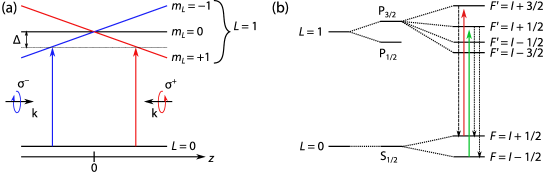
Figure 6: (a) Schematic for a one-dimensional MOT. Two beams with opposite circular polarizations (measured along $\hat{z}$) and zero-field detuning $\Delta$ are incident upon atoms in a magnetic field gradient (i.e, Eq. 15). The field is zero at $z=0$. This gradient splits the magnetic sublevels of the upper orbital angular momentum state into three. (b) Hierarchy of splittings of a realistic alkali-metal atom. The orbital angular momentum states $L=0$ (S) and $L=1$ (P) used in (a) are first split into states denoted by $L_{J}$ by spin-orbit interactions with total electronic angular momentum $J$. These levels are again split when the nuclear spin $I$ is coupled in via the hyperfine interaction to $J$, creating states of total atomic angular momentum $F$. One typically operates the MOT on the $F=I+1/2$ to $F^{\prime}=I+3/2$ transition (red arrow); however, because of off-resonant transitions between $F=I+1/2$ to $F^{\prime}=I+1/2$, a “repump” laser is added (green arrow). The dashed arrows show possible decay channels from excited states to the ground state manifold by spontaneous emission.

Here, we provide a brief explanation of magnetic-optical trapping and magnetic trapping, with a particular focus on the loading of atoms from one to the other. For a more thorough introduction, the interested reader can consult Refs. [36, 53].

MOTs cool and trap atoms by a combination of the Doppler effect and spatially varying light forces. The forces arise from light pressure: when an atom scatters a photon from a laser with wavevector $\mathbf{k}$, it receives a momentum kick $\hbar\mathbf{k}$. The characteristic timescale for this process is the excited state lifetime $1/\gamma$.

The typical MOT is depicted in Fig. 6a in one dimension for an atom with electronic orbital angular momentum $L=0$ in the ground state and $L^{\prime}=1$ in the excited state and projections $m_{L}$ of that angular momentum along this direction. First, consider an atom at some distance $+z$ with zero velocity. With the appropriately chosen polarizations, the right- (left-) going beam couples the $m_{L}=0$ to $m_{L}^{\prime}=+1$ ($m_{L}=0$ to $m_{L}^{\prime}=-1$), as indicated by the colors. The Zeeman effect due to the magnetic field gradient shifts the $m_{L}=0$ to $m_{L}^{\prime}=+1$ transition into resonance with the leftward going laser, while the rightward-going laser is shifted out of resonance with $m_{L}=0$ to $m_{L}^{\prime}=-1$ transition. This causes the atom to scatter photons from the leftward going beam and be pushed back toward the origin. The two laser beams interchange their roles for an atom placed at $-z$, causing the atom to be again pushed toward the origin. Second, consider the center of the trap where the magnetic field is zero and the $m^{\prime}_{L}$ levels are degenerate. (Figure 6a depicts a stationary atom.) If the atom is moving with velocity $+v$ ($-v$), the Doppler effect will shift the left (right) moving beam into resonance and the atom will scatter photons and be slowed. This is the slowing or cooling force of a MOT.

This picture is further complicated by the presence of additional angular momentum states in the atom, as shown in Fig. 6b. All alkali-metal-atom MOTs operate on an electron orbital angular momentum $L=0$ (S) to $L=1$ (P) transition. However, the atom also has an electron spin $S=1/2$, and the total electronic angular momentum is $\mathbf{J}=\mathbf{L}+\mathbf{S}$. This results in a single ground state with $J=1/2$ and two excited states with $J^{\prime}=1/2$ and $J^{\prime}=3/2$. The degeneracy of the two excited states is broken by spin-orbit coupling. This presents us a choice of whether to operate a MOT on the P_1/2 state (the D1 line) or P_3/2 state (the D2 line). In general, one wants the transitions driven in laser cooling to be “cycling” transitions: the excited state only decays back to the original ground state. This condition is most easily achieved on the $J=1/2$ to $J^{\prime}=3/2$ transition and, therefore, most MOTs operate on the D2 line.

This picture must also include the nuclear spin, which adds to $J$ to make a total angular momentum $\mathbf{F}=\mathbf{I}+\mathbf{J}$. For the ground state with $J=1/2$, this makes two states $F=I\pm 1/2$ (for $I>1/2$) that are split by the hyperfine interaction. For the excited $J^{\prime}=3/2$, it creates four states. The cycling transition is once again found on the $F=I+1/2$ to $F^{\prime}=I+3/2$ transition, which can only decay back to $F=I+1/2$ (see the dashed decay paths in Fig. 6b).

The hyperfine splitting in the excited state, however, is not sufficiently large compared to the excited state lifetime to completely prevent transitions between $F=I+1/2$ to $F^{\prime}=I+1/2$. If an atom is driven to this excited state, it can decay by spontaneous emission into either of the $F=I\pm 1/2$ ground states. Typically, as depicted in Fig. 6b, one must apply a second laser to “repump” the atoms out from $F=I-1/2$ back to $F=I+1/2$.

The repump laser can also be used to transfer atoms into a magnetic trap in a simple way. By merely turning off the repump laser, all atoms will eventually find themselves in the $F=I-1/2$ ground state. After this occurs, all lasers can be turned off and the atoms that happened to be pumped into the $m_{F}=-(I-1/2)$ state are magnetically trapped. This is the simplest means to load a magnetic trap from a MOT. By re-applying both lasers, the atoms trapped in the magnetic trap can be brought back into the MOT and counted.

References

References

- [1] Migdall A L, Prodan J V, Phillips W D, Bergeman T H and Metcalf H J 1985 Phys. Rev. Lett. 54 2596
- [2] Bjorkholm J E 1988 Phys. Rev. A 38 1599
- [3] Willems P A and Libbrecht K G 1995 Phys. Rev. A 51 1403
- [4] O’Hara K M, Granade S R, Gehm M E, Savard T A, Bali S, Freed C and Thomas J E 1999 Phys. Rev. Lett. 82 4204
- [5] Arpornthip T, Sackett C A and Hughes K J 2012 Phys. Rev. A 85 033420
- [6] Yuan J P, Ji Z H, Zhao Y T, Chang X F, Xiao L T and Jia S T 2013 Appl. Opt. 52 6195
- [7] Booth J L, Fagnan D E, Klappauf B G, Madison K W and Wang J 2014 US Patent 8803072B2
- [8] Moore R W G, Lee L A, Findlay E A, Torralbo-Campo L, Bruce G D and Cassettari D 2015 Rev. Sci. Instrum. 86 093108
- [9] Makhalov V B, Martiyanov K A and Turlapov A V 2016 Metrologia 53 1287
- [10] Scherschligt J, Fedchak J A, Barker D S, Eckel S, Klimov N, Makrides C and Tiesinga E 2017 Metrologia 54 S125
- [11] Hauth M, Freier C, Schkolnik V, Senger A, Schmidt M and Peters A 2013 Appl. Phys. B 113 49
- [12] Rushton J A, Aldous M and Himsworth M D 2014 Rev. Sci. Instrum. 85 121501
- [13] Bayard R T and Alpert D 1950 Rev. Sci. Instrum. 21 571
- [14] Redhead P A 1966 J. Vac. Sci. and Technol. 3 173
- [15] Arnold P C, Bills D G, Borenstein M D and Borichevsky S C 1994 J. Vac. Sci. and Technol. A 12 580
- [16] Lee J, Grover J A, Orozco L A and Rolston S L 2013 J. Opt. Soc. Am. B 30 2869
- [17] Nshii C C, Vangeleyn M, Cotter J P, Griffin P F, Hinds E A, Ironside C N, See P, Sinclair A G, Riis E and Arnold A S 2013 Nat. Nanotechnol. 8 321
- [18] Vangeleyn M, Griffin P F, Riis E and Arnold A S 2009 Opt. Express 17 13601
- [19] Lee K I, Kim J a, Noh H R and Jhe W 1996 Opt. Lett. 21 1177
- [20] Zhu C, Dalgarno A and Derevianko A 2002 Phys. Rev. A 65 034708
- [21] Jiang J, Mitroy J, Cheng Y and Bromley M W 2015 At. Data Nucl. Data Tables 101 158
- [22] Tao J, Perdew J P and Ruzsinszky A 2012 Proc. Natl. Acad. Sci. 109 18
- [23] Child M 2014 Molecular Collision Theory Dover Books on Chemistry (New York: Dover)
- [24] Landau L and Lifshitz E 2013 Quantum Mechanics: Non-Relativistic Theory Course of Theoretical Physics (Amsterdam: Elsevier)
- [25] Derevianko A, Porsev S G and Babb J F 2010 At. Data Nucl. Data Tables 96 323
- [26] Tang L Y, Yan Z C, Shi T Y and Mitroy J 2010 Phys. Rev. A 81 042521
- [27] Safronova M S and Safronova U I 2011 Phys. Rev. A 83 052508
- [28] Mata R A, Cabral B J C, Millot C, Coutinho K and Canuto S 2009 J. Chem. Phys. 130 014505
- [29] Oddershede J and Svendsen E 1982 Chem. Phys. 64 359
- [30] Hohm U 1994 Chem. Phys. 179 533
- [31] Bali S, O’Hara K M, Gehm M E, Granade S R and Thomas J E 1999 Phys. Rev. A 60 R29
- [32] Fagnan D E, Wang J, Zhu C, Djuricanin P, Klappauf B G, Booth J L and Madison K W 2009 Phys. Rev. A 80 022712
- [33] Hoffmann D, Bali S and Walker T 1996 Phys. Rev. A 54 R1030
- [34] Van Dongen J, Zhu C, Clement D, Dufour G, Booth J L and Madison K W 2011 Phys. Rev. A 84 022708
- [35] Ritchie N W M, Abraham E R I and Hulet R G 1994 Laser Phys. 4 1066
- [36] Foot C 2005 Atomic Physics Oxford Master Series in Physics (Oxford: Oxford University Press)
- [37] Vangeleyn M 2011 Atom trapping in non-trivial geometries for micro-fabrication applications Ph.D. thesis University of Strathclyde
- [38] Gallagher A and Pritchard D E 1989 Phys. Rev. Lett. 63 957
- [39] Sesko D, Walker T, Monroe C, Gallagher A and Wieman C 1989 Phys. Rev. Lett. 63 961
- [40] Kawanaka J, Shimizu K, Takuma H and Shimizu F 1993 Phys. Rev. A 48 R883
- [41] Browaeys A, Poupard J, Robert A, Nowak S, Rooijakkers W, Arimondo E, Marcassa L, Boiron D, Westbrook C I and Aspect A 2000 Eur. Phys. J. D 8 199
- [42] Petrich W, Anderson M H, Ensher J R and Cornell E A 1995 Phys. Rev. Lett. 74 3352
- [43] Alcock C B, Itkin V P and Horrigan M K 1984 Can. Metall. Q. 23 309
- [44] Haynes W M 2016 CRC handbook of chemistry and physics: a ready-reference book of chemical and physical data 97th ed (Boca Rotan: CRC Press)
- [45] Norrgard E B, Barker D S, Fedchak J A, Klimov N, Scherschligt J and Eckel S 2018 Rev. Sci. Instrum. 89 056101
- [46] Erjavec B and Setina J 2011 J. Vac. Sci. Technolog. A 29 051602
- [47] Bansod T, Sindal B K, Kumar K and Shukla S K 1998 J. Phys.: Conf. Ser. 390 012023
- [48] Barker D S, Norrgard E B, Scherschligt J, Fedchak J A and Eckel S 2018 [arXiv:1805.09862]
- [49] Halama H J and Foerster C L 1991 Vacuum 42 185
- [50] Herbeaux C, Marin P, Baglin V and Gröbner O 1999 J. Vac. Sci. Technolog. A 17 635
- [51] Koebley S R, Outlaw R A and Dellwo R R 2012 J. Vac. Sci. Technolog. A 30 060601
- [52] Kang S, Mott R P, Gilmore K A, Sorenson L D, Rakher M T, Donley E A, Kitching J o and Roper C S 2017 App. Phys. Lett. 110 244101
- [53] Metcalf H and van der Straten P 2012 Laser Cooling and Trapping Graduate Texts in Contemporary Physics (New York: Springer)