Non-Gibbs states on a Bose-Hubbard lattice

Abstract

We study the equilibrium properties of the repulsive quantum Bose-Hubbard model at high temperatures in arbitrary dimensions, with and without disorder. In its microcanonical setting the model conserves energy and particle number. The microcanonical dynamics is characterized by a pair of two densities: energy density $\varepsilon$ and particle number density $n$. The macrocanonical Gibbs distribution also depends on two parameters: the inverse nonnegative temperature $\beta$ and the chemical potential $\mu$. We prove the existence of non-Gibbs states, that is, pairs $(\varepsilon,n)$ which cannot be mapped onto $(\beta,\mu)$. The separation line in the density control parameter space between Gibbs and non-Gibbs states $\varepsilon\sim n^{2}$ corresponds to infinite temperature $\beta=0$. The non-Gibbs phase cannot be cured into a Gibbs one within the standard Gibbs formalism using negative temperatures.

I Introduction

Equipartition, ergodicity, and thermalization are essential properties, which an isolated many-body system has to have in order to qualify for the applicability of fundamental laws of statistical mechanics. Violation of the former, on the other side, could preserve coherence and might be of interest for, e.g., efficient information processing on classical and quantum levels. Surprising indications of transitions from ergodic to nonergodic dynamics have been reported in models of Josephson junction chains Pino et al. (2016) and Bose-Einstein condensates of ultracold atoms on optical lattices Mithun et al. (2018) upon “heating” the systems, i.e., upon increasing the average unbounded energy density.

For a macroscopic system with the energy being the only relevant conserved quantity — as in the case of the Josephson junction network Pino et al. (2016) — the canonical distribution function allows us to map any average energy density $\varepsilon$ into a positive inverse temperature $\beta$ of the canonical distribution .

In the presence of a second conserved quantity (e.g., the particle number) the situation changes. The additional constraint unfolds the existence of a non-Gibbs statistics of the one-dimensional Gross-Pitaevskii (GP) lattice also known as the discrete nonlinear Schrödinger equation with Hamiltonian

$$H=\sum_{l}-J\left(\psi_{l}^{*}\psi_{l+1}+\mathrm{c.c.}\right)+\frac{U}{2}|\psi_{l}|^{4}$$ (1)

and the Hamiltonian equations of motion $i\dot{\psi}_{l}=\partial H/\partial\psi_{l}^{*}$, as obtained in Ref. Rasmussen et al. (2000). The GP dynamics preserves the energy $H$ and the total norm $N=\sum_{l}|\psi_{l}|^{2}$. The microcanonical dynamics at equilibrium — if existent — is defined by the two densities $\varepsilon=H/M$ and $n=N/M$, where $M$ is the number of lattice sites not . In the macroscopic limit $M\rightarrow\infty$ it follows that the Gibbs grand-canonical formalism becomes only applicable to the microcanonical dynamics for energy densities $\varepsilon\leqslant Un^{2}$, despite the fact that the microcanonical dynamics can address states with $\varepsilon>Un^{2}$. These states are therefore called non-Gibbs states Rasmussen et al. (2000). Subsequent studies addressed the question whether the microcanonical GP dynamics in the non-Gibbs phase is nonergodic Rumpf and Newell (2001); Rumpf (2004, 2007, 2008, 2009); Buonsante et al. (2017). Recent data Mithun et al. (2018) show that the dynamics stays ergodic; however, relaxation times quickly grow deep in the non-Gibbs phase, turning the system into a dynamical glass, which becomes quickly nonergodic for any practical purpose. The microscopic mechanism is related to the excitation of long-lived discrete breathers Flach and Willis (1998); Flach and Gorbach (2008). These discrete breathers become precise single-action excitations of the system in the infinite density limit, where the GP system turns into an integrable set of uncoupled anharmonic oscillators. The anomalously growing lifetime of these objects is the reason for the growth of relaxation times Mithun et al. (2018).

In this work we consider the corresponding quantum model, the Bose-Hubbard model on lattices with arbitrary dimension $d$ (note that the particular choice of lattice symmetry will not be of importance) Fisher et al. (1989). For simplicity we only show here its direct one-dimensional nearest-neighbour counterpart of the GP lattice (1):

$$\hat{H}=\sum_{l}-J\left(\hat{a}_{l}^{\dagger}\hat{a}_{l+1}+\mathrm{H.c.}\right)+\frac{U}{2}\hat{n}_{l}\left(\hat{n}_{l}-1\right).$$ (2)

Here, $\hat{a}_{l}^{\dagger}$ and $\hat{a}_{l}$ are the bosonic creation and annihilation operators on the $l$th lattice site with the commutation relations $[\hat{a}_{i},\hat{a}_{j}^{{\dagger}}]=\delta_{ij}$, and $\hat{n}_{l}=\hat{a}_{l}^{\dagger}\hat{a}_{l}$ is the site occupation number. The GP Hamiltonian (1) is the classical limit of the Bose-Hubbard (BH) Hamiltonian (2) for large occupation numbers $n_{l}\gg 1$, since quantum operators can be replaced by $c$-numbers: $\hat{a}_{i}\to\psi_{i}$, $\hat{a}_{i}^{{\dagger}}\to\psi_{i}^{*}$.

We will show that the non-Gibbs phase exists in the full quantum BH lattice model as well for energy densities $\varepsilon>Un^{2}$ in the $n$-$\varepsilon$ plane, where $n=N/M$ and $\varepsilon=E/M$ are the average occupation number (filling factor) and energy per site, respectively, and $U\geqslant 0$ is the on-site repulsion energy of the BH lattice Hamiltonian Fisher et al. (1989). We will also generalize to disorder potentials. Our general proof of the existence of nonthermal non-Gibbs states is relevant for a variety of experimental setups of Bose-Einstein condensates of ultracold atomic gases in optical lattice potentials, which are often used to study fundamental properties of matter Bloch et al. (2008).

This paper is organized as follows: in Sec. II, we obtain the line of infinite temperatures and, by means of the method of cumulant expansions, the thermodynamic susceptibilities for the Bose-Hubbard model. In the next section, we generalize these results to the Bose-Hubbard model with disorder (Sec. III.1) and with arbitrary local interactions (Sec. III.4). We consider the density of states of the system near the infinite temperature line and discuss the important role of boundedness of the single-particle spectrum. In the Conclusions, we review the obtained results and discuss possible applications and prospects.

II Main results

II.1 The method

The limiting line $\varepsilon=Un^{2}$, found in Ref. Rasmussen et al. (2000), corresponds to infinite temperatures of the canonical Gibbs ensemble. However, the non-Gibbs region above the line in the $n$-$\varepsilon$ parameter space is experimentally (numerically) accessible, since it is possible to initialize the lattice at any energy and total number of particles Rasmussen et al. (2000); Flach and Gorbach (2008). For instance, putting all $N$ bosons onto one site gives the energy per site $\varepsilon\sim N\sim M$, which is infinitely large in the thermodynamic limit. Dissipative boundaries were also proposed in order to drive the system into a non-Gibbs region Livi et al. (2006); Iubini et al. (2013). Here we address the question whether the limiting line also exists in the quantum Bose-Hubbard model and which equation it obeys.

In order to answer this question, we calculate the average energy in the canonical ensemble, that is, the internal energy as a function of the temperature, total number of particles, and the number of lattice sites, $E=\langle\hat{H}\rangle=E\left(T,N,M\right)=M\varepsilon\left(T,n\right)$. The last equality is valid in the thermodynamic limit, because the internal energy and total number of particles are extensive properties of the system. The Gibbs canonical ensemble is, conceptually, the most convenient one to study this problem, because we know the full range of values of thermodynamic variables $T$ and $n$. For a given density $n$ and for $0\leqslant T<\infty$, the line $\varepsilon\left(T,n\right)$ goes through all possible values of $\varepsilon$ in the $n$-$\varepsilon$ plane. The capacity

$$\left(\partial E/\partial T\right)_{N,M}=M\left(\partial\varepsilon/\partial T\right)_{n}$$ (3)

is positive, which implies that the energy reaches its maximum for $T\to+\infty$, and, therefore, $\varepsilon(n)=\lim_{T\to+\infty}\varepsilon\left(T,n\right)$ is the upper bound for the Gibbs region in the $n$-$\varepsilon$ plane, provided the limit exists.

The grand canonical potential is defined as $\Omega=\Omega\left(T,\mu,M\right)=E-TS-\mu N$ with $S$ being the entropy, and $\mu=\left(\partial E/\partial N\right)_{T,M}=\left(\partial\varepsilon/\partial n\right)_{T}$ is the chemical potential. Below we use two independent variables $\beta\equiv 1/T$ and $\alpha\equiv-\beta\mu$ instead of $T$ and $\mu$ to simplify calculations. For the grand canonical Gibbs ensemble, the partition function $Z\left(\beta,\alpha,M\right)=\exp\left(-\beta\Omega\right)$ is given by

$$Z\left(\beta,\alpha,M\right)=\mathop{\mathrm{Tr}}\exp\left(-\beta\hat{H}-\alpha\hat{N}\right).$$ (4)

Then the internal energy and total number of particles per site take the form

$$\varepsilon\left(\beta,\alpha\right) =-\frac{1}{M}\frac{\partial\ln Z\left(\beta,\alpha,M\right)}{\partial\beta},$$ (5)

$$n\left(\beta,\alpha\right) =-\frac{1}{M}\frac{\partial\ln Z\left(\beta,\alpha,M\right)}{\partial\alpha}.$$ (6)

The grand canonical ensemble is equivalent to the canonical one only for nonzero susceptibility $\left(\partial N/\partial\mu\right)_{\beta}$, since otherwise the chemical potential is not a well-defined function of $n$. The susceptibility vanishes at low temperatures for the Bose Hubbard model when the on-site repulsion $U/J$ is sufficiently large Fisher et al. (1989). As a consequence the system becomes a Mott insulator with zero compressibility. However, at high temperatures, the susceptibility is not zero, as shown below.

Excluding the variable $\alpha$ from Eqs. (5) and (6) yields $\varepsilon$ as a function of temperature and filling factor and hence the particular case $\varepsilon=\varepsilon(n)$ at $\beta=0$, which we are interested in.

II.2 Perturbation series at high temperatures

For the GP lattice, the value $\alpha\left(\beta,n\right)=-\beta\mu\left(\beta,n\right)$ is shown to be finite and positive in the limit $\beta\to 0$  Rasmussen et al. (2000). We assume that this property is also valid for the BH model and then show the consistency of the assumption. Thus, the fugacity $z={e}^{\beta\mu}={e}^{-\alpha}$ (see, e.g., Ref. Huang (1987)) will tend to a constant value less than one in the same limit.

In order to obtain a perturbation series at high temperatures for the grand partition function, one can use the commutativity $\hat{H}$ and $\hat{N}=\sum_{i}\hat{n}_{i}$ and expand $\exp\left(-\beta\hat{H}\right)$ in a power series in the inverse temperature

$$Z(\beta,\alpha, M)=\mathop{\mathrm{Tr}}\left[\left(1-\beta\hat{H}+\beta^{2}\hat{H}^{2}/2+\cdots\right)\exp\left(-\alpha\hat{N}\right)\right]$$

$$=Z_{0}\left(\alpha,M\right)\left(1-\beta\big{\langle}\hat{H}\big{\rangle}_{0}+\beta^{2}\big{\langle}\hat{H}^{2}\big{\rangle}_{0}/2+\cdots\right)$$ (7)

thus arriving at the expansion with the statistical moments $\mu_{m}\equiv\big{\langle}\hat{H}^{m}\big{\rangle}_{0}$. Here we denote $Z_{0}\left(\alpha,M\right)=\mathop{\mathrm{Tr}}\exp\left(-\alpha\hat{N}\right)$ and the brackets $\big{\langle}\cdots\big{\rangle}_{0}=\mathop{\mathrm{Tr}}\left(\cdots\hat{\rho}_{0}\right)$ stand for the average over the density matrix in the zero-order approximation

$$\hat{\rho}_{0}=\frac{\exp\left(-\alpha\sum_{i}\hat{n}_{i}\right)}{Z_{0}\left(\alpha,M\right)}.$$ (8)

The usage of the moment expansion is not convenient, since $\ln Z\left(\beta,\alpha,M\right)$ should be proportional to $M$ in the thermodynamic limit, while the moment $\mu_{m}$ is proportional to $M^{m}$. In order to solve this problem, we reexpand $\ln\left(1-\beta\mu_{1}+\beta^{2}\mu_{2}/2!-\beta^{3}\mu_{3}/3!+\cdots\right)$ in powers of $\beta$ thus arriving at the cumulant expansion with respect to $-\beta$ Rushbrooke et al. (1974)

$$\ln Z\left(\beta,\alpha,M\right)=\lambda_{0}-\beta\frac{\lambda_{1}}{1!}+\beta^{2}\frac{\lambda_{2}}{2!}-\beta^{3}\frac{\lambda_{3}}{3!}+\cdots$$ (9)

where each cumulant $\lambda_{i}$ depends on $\alpha$ and $M$, and $\lambda_{0}=\ln Z_{0}\left(\alpha,M\right)$. Cumulants can be obtained from the moments

$$\lambda_{1}=\mu_{1},\ \lambda_{2}=\mu_{2}-\mu_{1}^{2},\ \lambda_{3}=\mu_{3}-3\mu_{1}\mu_{2}+2\mu_{1}^{3},$$ (10)

and so on. Since $\ln Z$ and all its derivatives with respect to $\beta$ are proportional to $M$ in the thermodynamic limit, the terms of order $M^{2}$ and higher cancel each other, and each cumulant turns out to be proportional to $M$.

When calculating the energy per site at infinite temperatures, it is sufficient to restrict ourselves to the first cumulant. For obtaining the capacity (3), we need the second order expansion

$$\ln Z\left(\beta,\alpha,M\right)= \ln Z_{0}\left(\alpha,M\right)-\beta\big{\langle}\hat{H}\big{\rangle}_{0}$$

$$+\beta^{2}\left(\big{\langle}\hat{H}^{2}\big{\rangle}_{0}-\big{\langle}\hat{H}\big{\rangle}_{0}^{2}\right)/2+\cdots.$$ (11)

II.3 The high-temperature expansion for the Bose-Hubbard model

We calculate the partition function in the zero-order approximation in the Fock basis $\Ket{\ldots,n_{i},\ldots}$ for the operators $\hat{a}_{i}$ and $\hat{a}_{i}^{{\dagger}}$, where the density matrix is diagonal,

$$Z_{0}\left(\alpha,M\right)=\left[\sum_{n_{i}=0}^{\infty}\exp\left(-\alpha n_{i}\right)\right]^{M}=\frac{1}{\left(1-{e}^{-\alpha}\right)^{M}}.$$ (12)

Since the density matrix (8) is the exponential of a quadratic form of the bosonic operators $\hat{a}_{i}^{{\dagger}}$ and $\hat{a}_{i}$, the Wick-Bloch-De Dominicis theorem Bloch and Dominicis (1958) can be applied for calculating the average of a product of an arbitrary number of bosonic operators. According to the theorem, this average is given by the complete sum of all possible products of elementary binary averages (contractions)

$$\langle\hat{a}_{i}^{\dagger}\hat{a}_{j}\rangle_{0} =\delta_{ij}n_{0}.$$ (13)

Here $n_{0}$ is the mean occupation number per site (lattice filling factor) at $\beta=0$,

$$n_{0}=\langle\hat{a}_{i}^{\dagger}\hat{a}_{i}\rangle_{0}=\left(1-{e}^{-\alpha}\right)\sum_{k=0}^{\infty}k\,{e}^{-\alpha k}=\frac{1}{{e}^{\alpha}-1},$$ (14)

and the “nondiagonal” values are zero, since the average $\Braket{\ldots,n_{k},\ldots}{\hat{a}_{j}^{\dagger}\hat{a}_{i}}{\ldots,n_{k},\ldots}$ vanishes for $i\neq{}j$.

The mean value of the energy (2) at $\beta=0$ is obtained as follows. The hopping terms in $\big{\langle}\hat{H}\big{\rangle}_{0}$ vanish, since they include only nondiagonal binary terms. We are left only with the interaction energy terms, for which in accordance with the Wick–Bloch–De Dominicis theorem, $\langle\hat{a}_{i}^{\dagger 2}\hat{a}_{i}^{2}\rangle_{0}=2\langle\hat{a}_{i}^{\dagger}\hat{a}_{i}\rangle_{0}^{2}=2n_{0}^{2}$. Thus

$$\big{\langle}\hat{H}\big{\rangle}_{0}={MU}n_{0}^{2}.$$ (15)

We substitute Eqs. (12) and (15) into Eq. (11) and use Eqs. (5) and (6) to derive

$$\varepsilon ={U}{n_{0}^{2}}+{O}\left(\beta\right),$$ (16)

$$n =n_{0}[1-2\beta Un_{0}(n_{0}+1)]+{O}\left(\beta^{2}\right).$$ (17)

Here the symbol ${O}\left(x\right)$ denotes terms of order $x$ and higher.

This system of equations allows us to obtain the upper border for the Gibbs region in the $n$-$\varepsilon$ plane. For infinite temperatures, we have $n=n_{0}$ and

$$\varepsilon=Un^{2},$$ (18)

which is the main result of this work. It coincides with the Gibbs–non-Gibbs border for the discrete nonlinear Schrödinger equation Rasmussen et al. (2000).

In the limit of infinite temperatures, the average energy per particle (18) is finite at fixed particle density. In the same limit, the density matrix (8) is independent of the energy, which makes all energies equiprobable at a fixed particle density. On the other hand, the upper bound of the spectrum of the Bose-Hubbard Hamiltonian grows as $M^{2}$, which seemingly leads to a divergence of the average energy in the thermodynamic limit. The resolution of this apparent paradox is that the density of states decreases rapidly at high energies.

Equations (14) and (17) yield the parameter $\alpha$ up to the first-order term proportional to $\beta$:

$$\mu=-\frac{1}{\beta}\ln\left(1+1/n\right)+2Un+{O}\left(\beta\right)$$ (19)

which leads to

$$\left(\frac{\partial\mu}{\partial n}\right)_{\beta}=\frac{1}{\beta n\left(n+1\right)}+2U+{O}\left(\beta\right).$$ (20)

The quantity (20) is directly related to the fluctuations of the total number of particles in the grand canonical ensemble, which remain finite in the limit of infinite temperatures,

$$\frac{\big{\langle}\hat{N}^{2}\big{\rangle}-\big{\langle}\hat{N}\big{\rangle}^{2}}{\big{\langle}\hat{N}\big{\rangle}}= \frac{1}{\beta n}\left(\frac{\partial n}{\partial\mu}\right)_{\beta}=(n+1)$$

$$\times\left[1-2\beta n(n+1)U+O(\beta^{2})\right].$$ (21)

In order to obtain the capacity (3), we have to consider the second-order terms in Eq. (11). In the same manner as for Eq. (15), we derive

$$\big{\langle}\hat{H}^{2}\big{\rangle}_{0}-\big{\langle}\hat{H}\big{\rangle}_{0}^{2}=Mn_{0}\left(n_{0}+1\right)\left[2J^{2}d+U^{2}n_{0}\left(5n_{0}+1\right)\right],$$ (22)

where $d$ is the dimension of the lattice. We rewrite the capacity per site in the more convenient form

$$\left(\frac{\partial\varepsilon}{\partial T}\right)_{n}=-\beta^{2}\left(\frac{\partial\varepsilon}{\partial\beta}\right)_{n}=-\frac{\beta^{2}}{\left(\frac{\partial n}{\partial\alpha}\right)_{\beta}}\frac{\partial\left(\varepsilon,n\right)}{\partial\left(\beta,\alpha\right)},$$ (23)

where we use the standard thermodynamic notation for the Jacobian determinant. By means of Eqs. (11)–(15) and (22), we arrive at the capacity per site in the lowest order in $\beta$

$$\left(\frac{\partial\varepsilon}{\partial T}\right)_{n}=\beta^{2}n\left(n+1\right)\left[2J^{2}d+U^{2}n\left(n+1\right)\right]+{O}\left(\beta^{3}\right),$$ (24)

which is positive for any nonzero $\beta$ and turns zero at infinite temperature.

The positiveness of the expressions (21) and (24) implies that the system is stable at high temperatures.

The classical limit of the BH model, that is, the classical GP lattice can be evaluated in a similar manner for arbitrary lattice dimension by replacing sums by corresponding integrals. However, it is simpler to find the thermodynamic relations by considering the classical limit $n\gg 1$ in the obtained quantum system equations. For instance, Eq. (14) becomes in this limit $n_{0}=1/\alpha$, and therefore, $n=1/\alpha$ at infinite temperatures in the classical case (see the discussion in Sec. III.4.2 below). Similarly we can replace $n(n+1)$ by $n^{2}$ in the equations for the susceptibility (20) and capacity (24), in order to find their classical limits. We note that the thermodynamic relations of the quantum and classical cases differ significantly for small particle densities.

Let us emphasize that the classical limit is not realized by a quantum system at infinite temperatures. Even on the infinite temperature line, the relation between the density of particles and fugacity ($z={e}^{-\alpha}$) varies: in the quantum model $n=z/(1-z)$, while in the classical one, $n=-1/\ln z$. This is because the energy remains finite in the limit of infinite temperatures at a given particle density. Note that the classical case can be obtained from the quantum one in the limit $n\gg 1$, but an inverse scheme does not exist.

III Generalizations

III.1 Adding disorder

Let us consider the Bose-Hubbard model with disorder by adding to the Hamiltonian (2) a disorder potential $\hat{H}_{\mathrm{dis}}=\sum_{i}\epsilon_{i}\hat{a}_{i}^{\dagger}\hat{a}_{i}$ with random on-site energies $\epsilon_{i}$, obeying some probability density distribution (see, e.g., Ref. Flach (2016)). Their average value $\overline{\epsilon}=\lim_{M\to\infty}M^{-1}\sum_{i}\epsilon_{i}$ is assumed to be zero, while the variance $\sigma_{\epsilon}$ is finite.

The disorder potential does not change the upper bound for the Gibbs region (18). Its contribution to the energy per site is equal to zero in the limit of infinite temperatures: $\big{\langle}\hat{H}_{\mathrm{dis}}\big{\rangle}_{0}=n_{0}M^{-1}\sum_{i}\epsilon_{i}=0$. However, the presence of disorder influences the second-order term in the high temperature expansion (11) into

$$\big{\langle}\hat{H}^{2}\big{\rangle}_{0}-\big{\langle}\hat{H}\big{\rangle}_{0}^{2}= Mn_{0}\left(n_{0}+1\right)$$

$$\times\left[\sigma_{\epsilon}+2J^{2}d+U^{2}n_{0}\left(5n_{0}+1\right)\right],$$ (25)

and, hence, the capacity per site

$$\left(\frac{\partial\varepsilon}{\partial T}\right)_{n}\!\!=\beta^{2}f(n)+{O}\left(\beta^{3}\right),$$ (26)

where we use the notation

$$f(n)=n\left(n+1\right)\left[\sigma_{\epsilon}+2J^{2}d+U^{2}n\left(n+1\right)\right].$$ (27)

The border of the Gibbs region and the capacity at high temperatures are independent of the correlations in disorder $\big{\langle}\epsilon_{i}\epsilon_{i+m}\big{\rangle}=\lim_{M\to\infty}M^{-1}\sum_{i}\epsilon_{i}\epsilon_{i+m}$ for $m\neq 0$. Therefore uncorrelated disorder with finite variance will result in the same border between the Gibbs and the non-Gibbs regime given by (LABEL:enborder). This result holds independent of the dimensionality of the lattice, and generalizes the previously obtained consideration of a one-dimensional disordered GP lattice Flach (2016).

III.2 The density of states in the vicinity of the Gibbs - non-Gibbs separation line

Let us calculate the density of states in the vicinity of the border separating the Gibbs and non-Gibbs states. Instead of following the route by calculating the entropy near $\beta=0$ by means of the grand canonical potential: $S(T,\mu,M)=-(\partial\Omega/\partial T)_{\mu,M}$, we use Eq. (26) for the capacity, since entropy and capacity per site are related by the equation $(\partial\varepsilon/\partial T)_{n}=T(\partial s/\partial T)_{n}$. Then the expression (26) leads to $(\partial s/\partial\beta)_{n}=-\beta f(n)$ and after integration over $\beta$ to

$$s=s_{0}(n)-\frac{\beta^{2}}{2}f(n)+{O}\left(\beta^{3}\right)$$ (28)

with $s_{0}(n)$ being the entropy per site at infinite temperature

$$s_{0}(n)=(n+1)\ln(n+1)-n\ln n.$$ (29)

The last equation can be obtained directly from the density matrix (8) using the well-known relation for the entropy, $S_{0}=-\mathop{\mathrm{Tr}}\hat{\rho}_{0}\ln\hat{\rho}_{0}$.

In the same manner, we derive from Eqs. (18) and (26)

$$\varepsilon=Un^{2}-\beta f(n)+{O}\left(\beta^{2}\right).$$ (30)

Excluding the inverse temperature from Eqs. (28) and (30) yields

$$s=(n+1)\ln(n+1)-n\ln n-\frac{\big{(}\varepsilon-Un^{2}\big{)}^{2}}{2f(n)},$$ (31)

where $f(n)$ is given by Eq. (27). By using the relation $W={e}^{S}={e}^{sM}$, we arrive at the density of states in the microcanonical ensemble near the Gibbs - non-Gibbs border

$$W(E,N,M)=\frac{(M+N)^{M+N}}{N^{N}M^{M}}\exp\left[-\frac{M\big{(}\varepsilon-Un^{2}\big{)}^{2}}{2f(n)}\right],$$ (32)

where $n=N/M$ and $\varepsilon=E/M$. This is the main contribution to the asymptotics of the density of states in the thermodynamic limit $N/M=\mathrm{const}$, $M\to\infty$. The density of states reaches its maximum precisely at the border $\varepsilon=Un^{2}$.

The density of states for the discrete GP Hamiltonian (1)

$$W_{\mathrm{cl}}(E,N,M)=\left(\frac{N{e}}{M}\right)^{M}\exp\left[-\frac{M\big{(}\varepsilon-Un^{2}\big{)}^{2}}{2f_{\mathrm{cl}}(n)}\right],$$ (33)

can be inferred from Eq. (32) in the classical limit $n\gg 1$, where $f_{\mathrm{cl}}(n)=n^{2}\left(\sigma_{\epsilon}+2J^{2}d+U^{2}n^{2}\right)$. In the particular case $U=0$ (the ideal Bose gas), the parabolic dependence of the entropy on the energy in the microcanonical ensemble was obtained up to a coefficient in Ref. Buonsante et al. (2017) by another method.

Note that for both quantum and classical cases, the entropy is monotonously increasing with $n$ at fixed $\varepsilon$, while it is nonmonotonous for increasing $\varepsilon$ at fixed $n$. This result is analogous to the one obtained in Ref. Rumpf (2004) for the one-dimensional classical GP lattice.

III.3 Bounded single particle spectra and non-Gibbs states

The Gibbs - non-Gibbs separation line (18) exists due to the single-particle dispersion being bounded, e.g., as $-2J\cos q$ for the one-band Bose-Hubbard model, (LABEL:BH). Note that generalizations to a finite number of bands generated by more complex lattice structures are straightforward. At variance, an infinite number of bands or the single-particle dispersion, or simply the case of free particle $q^{2}/2m$, leads to unbounded spectra. As a consequence non-Gibbs states are renormalized to infinite values in the $n$-$\varepsilon$ plane and vanish from any consideration. Indeed, in the particular case $U=0$, we have in general an ideal Bose gas with the dispersion $J_{\lambda}(q)$ with $\lambda$ being the band number. Then the total number of particles is given by the standard expression

$$N=\sum_{q,\lambda}1/\left[\exp\left(\beta J_{\lambda}(q)+\alpha\right)-1\right],$$ (34)

where the quasimomentum $q$ runs over $M$ uniformly distributed points in the Brillouin zone. In the case of a one-band structure, only one band, say, $\lambda=1$ contributes to the sum in (LABEL:multband). Then the limit $\beta\to 0$ yields $N=M/\left({e}^{\alpha}-1\right)$ which allows for a solution of $\alpha$ as a function of $n=N/M$. However, for an infinite number of bands, $\sum_{\lambda=1}^{\infty}1/\left({e}^{\alpha}-1\right)$ diverges. Therefore the assumption about the finiteness of $\alpha=-\beta\mu$ when $\beta\to 0$ is not applicable anymore.

III.4 Further extensions

Non-Gibbs states can be obtained as well for the following generalized Bose-Hubbard models

$$\hat{H}=\sum_{i\neq j}J\left(i-j\right)\hat{a}_{i}^{\dagger}\hat{a}_{j}+\sum_{i}u\left(\hat{n}_{i}\right).$$ (35)

The sum in the hopping term includes all sites, and the single particle dispersion $J\left(q\right)=\sum_{m}J\left(m\right){e}^{iqm}$ is assumed to be bounded. The standard Bose-Hubbard Hamiltonian (2) is a particular case of Eq. (35) with $J(m)=-J(\delta_{m,1}+\delta_{m,-1})$ and $u(x)=Ux(x-1)/2$.

If the condition

$$\lim_{x\rightarrow+\infty}\frac{u\left(x\right)}{x}\rightarrow+\infty$$ (36)

is satisfied, then a non-Gibbs phase with anomalous scaling properties of the energy will emerge. This phase cannot be described by a grand partition function with negative temperature due to the divergence of the former. If on the other side Eq.(36) is not satisfied, i.e., $\lim_{x\rightarrow\infty}u(x)/x\rightarrow C$ with $0\leqslant C<\infty$, then the line $\varepsilon\left(n,\beta=0\right)$ becomes the border between Gibbs states with positive and negative temperatures (see also Refs. Samuelsen et al. (2013); Buonsante et al. (2017)).

III.4.1 The Gibbs–non-Gibbs transition line for the generalized Bose-Hubbard model

By complete analogy with Sec. II.3, one can show that at infinite temperatures the hopping terms do not contribute to the average energy. Its value is determined by the interaction terms and calculated with the density matrix (8)

$$\varepsilon=(1-{e}^{-\alpha})\sum_{m=0}^{+\infty}u(m){e}^{-\alpha m}.$$ (37)

The density of particles is still given by Eq. (14). Substituting the exponential ${e}^{\alpha}=1+1/n$ into Eq. (37), we arrive at the curve of the energy density in the $\varepsilon$-$n$ plane

$$\varepsilon(n)=\frac{1}{n+1}\sum_{m=0}^{+\infty}u(m)\bigg{(}\frac{n}{n+1}\bigg{)}^{m},$$ (38)

above which non-Gibbs states for the Hamiltonian (35) emerge.

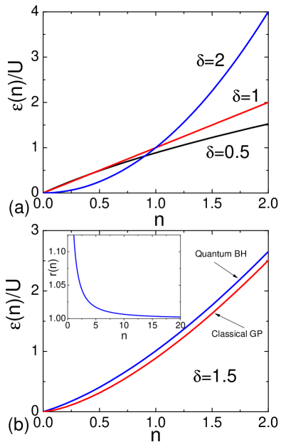
Figure 1: (Color online) (a) The infinite temperature line (40) in the $\varepsilon$-$n$ plane for the generalized Bose-Hubbard model (35) with the local potential of the power-law type (39) for different values of the exponent $\delta$. Here $\varepsilon$ and $n$ are the energy and particle densities, respectively. Non-Gibbs states are located above the line if $\delta>1$. At variance, for $\delta\leqslant 1$ the line separates states with positive and negative temperatures. Note that the case $\delta<1$ corresponds to a class of Bose systems with saturable interactions satisfying $u(x)\to\infty$ and $\partial u(x)/\partial x\to 0$ for $x\to\infty$. (b) The infinite temperature lines $\varepsilon_{q,c}(n)$ for the quantum (39) and classical (44) Bose-Hubbard and Gross-Pitaevskii models, respectively, as follows from Eqs. (40) and (41). The interaction potential is chosen with noninteger parameter $\delta=3/2$. Both lines differ at small densities, while their asymptotics for large $n$ coincides. Inset: The ratio $r(n)=\varepsilon_{q}(n)/\varepsilon_{c}(n)$ of the quantum versus classical critical energy density as a function of particle density.

As an example, we calculate the transition line for the local interaction energy

$$u(x)=\frac{U}{\delta}\bigg{[}\frac{\Gamma(x+1)}{\Gamma(x+1-\delta)}-\frac{1}{\Gamma(1-\delta)}\bigg{]}$$ (39)

with $\Gamma(x)$ being Euler’s gamma function. This form of the potential generalizes the power-law interaction $U\hat{a}^{\dagger m}\hat{a}^{m}/m$ on each site with a positive integer exponent $m$, for which $u(x)=Ux(x-1)\cdots(x-m+1)=\Gamma(x+1)/\Gamma(x+1-m)/m$. The last term in the right-hand side brackets in Eq. (39) is needed to enforce the condition $u(0)=0$, which the potential should satisfy for any positive $\delta$. The long-range asymptotics of that potential is given by $u(x)=Ux^{\delta}/\delta[1+O(1/x)]$. The line of infinite temperatures is calculated by means of Eq. (38), which yields

$$\varepsilon(n)=\frac{U}{\delta\Gamma(1-\delta)}\bigg{[}\frac{{}_{2}F_{1}(1,1;1-\delta;\frac{n}{n+1})}{n+1}-1\bigg{]},$$ (40)

where ${}_{2}F_{1}(a,b;c;z)$ is the hypergeometric function Abramowitz and Stegun (1974). As discussed above, this line separates the Gibbs and non-Gibbs phases when $\delta>1$. For positive integer exponent $\delta=1,2,\cdots$, Eq. (40) is simplified

$$\varepsilon(n)=U\Gamma(\delta)n^{\delta}.$$ (41)

This equation also gives the main term of the long-range asymptotics of Eq. (40) for arbitrary positive $\delta$. For the standard Bose-Hubbard model with two-body interactions, we have $\delta=2$ and arrive at Eq. (18) (see blue line in Fig. 1). For $\delta=1$ the impact of the potential is reduced to a renormalization of the chemical potential of a noninteracting ideal Bose gas (see red line in Fig. 1). As a result, this case separates the appearance of non-Gibbs phases for $\delta>1$ from cases with $\delta<1$, where the infinite temperature line separates Gibbs states with positive and negative temperatures (see black line in Fig. 1).

It is straightforward to extend the hopping network between sites. For instance, for binary interactions a one-band Hamiltonian takes the form

$$\hat{H}=\sum_{i\neq j}J\left(i-j\right)\hat{a}_{i}^{\dagger}\hat{a}_{j}+\frac{1}{2}\sum_{i,j}U\left(i-j\right)\hat{a}_{i}^{\dagger}\hat{a}_{j}^{\dagger}\hat{a}_{j}\hat{a}_{i}.$$ (42)

Using the same method as in Sec. II, we arrive at non-Gibbs states above the line $\varepsilon=U_{0}n^{2}$ with $U_{0}\equiv U(0)+\frac{1}{2}\sum_{j\not=0}U\left(j\right)$, which is assumed to be finite and positive.

Similar to Sec. III.1, we can show that the disorder does not modify the border line between Gibbs and non-Gibbs states for the both models, Eqs. (35) and (42).

III.4.2 The Gibbs–non-Gibbs transition line for the discrete nonlinear Schrödinger equation

We also consider the generalizations of the GP lattice (1), whose Hamiltonian is given by Eq. (35) with the replacement $\hat{a}_{i}\to\psi_{i}$, $\hat{a}_{i}^{{\dagger}}\to\psi_{i}^{*}$. One can calculate the Gibbs–non-Gibbs transition line in the same way as in Sec. II. However, the easiest way is to obtain it in the limit of large occupation numbers, when the quantum model approaches the classical one. Then the density of particles in Eq. (14) is $n=1/\alpha$ and the sum in Eq. (37) tends to the integral $\int_{0}^{\infty}\mathrm{d}xu(x)\exp(-\alpha x)/\alpha$. We finally obtain

$$\varepsilon(n)=\frac{1}{n}\int_{0}^{\infty}u\left(x\right){e}^{-x/n}\mathrm{d}x.$$ (43)

We observe that the line of infinite temperatures $\varepsilon(n)$ is given by the Laplace transform $F(s)$ of the interaction potential $u(x)$ through $\varepsilon(n)=sF(s)|_{s=1/n}$. Similar to the quantum case, non-Gibbs states for the Hamiltonian (35) emerge for energy densities $\varepsilon>\varepsilon(n)$ if the condition (36) is satisfied.

The classical analog of the potential (39) in the Bose-Hubbard model is

$$u(x)=Ux^{\delta}/\delta.$$ (44)

Using Eq. (43), we find the Gibbs–non-Gibbs separation line given by Eq. (41). Thus, for an integer exponent $\delta$, the infinite temperature line for the quantum and classical models is identical, but for noninteger $\delta$ it is not, see Fig. 1b.

One can see that for the interaction $\sum_{i}:\!u\left(\hat{n}_{i}\right)\!:$ with $u(x)$ being an entire function of $x$, the line $\beta=0$ matches Eq. (43). Here the symbols $:\!\cdots\!:$ stand for the normal ordering of the Bose operators $\hat{a}_{i}$ and $\hat{a}_{i}^{\dagger}$. In order to prove this equation, it is sufficient to expand an arbitrary function $u\left(x\right)$ in a Taylor series and show the equation validity for each term of the series. Thus, we consider the particular case $u\left(x\right)=x^{m}$ for any nonnegative integer $m$, for which $:\!\hat{n}^{m}\!:=\hat{a}^{\dagger m}\hat{a}^{m}$ (here we omit the lattice site index $i$ for simplicity). By applying the methods of Sec. II and using the Wick-Bloch-De Dominicis theorem, we arrive at $\varepsilon=\big{\langle}\hat{a}^{\dagger m}\hat{a}^{m}\big{\rangle}_{0}=m!n_{0}^{m}=m!n^{m}$. The last equality is valid in zeroth order in $\beta$. This coincides with the relation $\varepsilon=m!n^{m}$ given by Eq. (43).

Samuelsen et al. Samuelsen et al. (2013) considered a one-dimensional chain with the saturable nonlinear potential $u\left(x\right)=\nu\ln\left(1+x\right)$ (with negative $\nu<0$), and obtained the line of infinite temperatures using a transfer integral approach:

$$\varepsilon=\nu\exp\left(1/n\right)E_{1}\left(1/n\right),$$ (45)

where $E_{1}\left(z\right)=\int_{z}^{\infty}\mathrm{d}t\,{e}^{-t}/t$ is the exponential integral Abramowitz and Stegun (1974). We note that our method is generating and therefore confirming that result using the above relation (43). We also note that our approach allows one to generalize the result (45) to arbitrary lattice dimensions.

III.5 The absence of the Gibbs–non-Gibbs transition line in a Josephson junction array model

Let us discuss why the Gibbs–non-Gibbs transition line is absent in a Josephson junction array

$$\hat{H}=\sum_{i}\frac{E_{\mathrm{C}}}{2}\hat{q}_{i}^{2}-E_{\mathrm{J}}\cos(\hat{\varphi}_{i}-\hat{\varphi}_{i+1}).$$ (46)

This is a simple model describing the Josephson junction network of weakly coupled superconducting islands with the Josephson $E_{\mathrm{J}}$ and charging $E_{\mathrm{C}}$ energies (see, e.g., Ref. Pino et al. (2016)). The operators of phase $\hat{\varphi}_{i}$ and charge $\hat{q}_{i}$ of the superconducting islands obey the commutation relations $[\hat{q}_{i},{e}^{i\hat{\varphi}_{j}}]=\delta_{ij}{e}^{i\hat{\varphi}_{j}}$. They can be considered as the $z$-component of momentum operators $\hat{q}_{i}\rightarrow\hat{l}_{zi}=-i\frac{\partial}{\partial\varphi_{i}}$ and $\hat{\varphi}_{i}\rightarrow\varphi_{i}$ on the ring of unit radius.

The Hamiltonian (46) is derived from the Bose-Hubbard model (2) in the limit of infinite densities Bruder et al. (2005). In the polar representation, the bosonic operators follow as

$$\hat{a}_{i}={e}^{-i\hat{\varphi}_{i}}\sqrt{n+\delta\hat{n}_{i}},\quad\hat{a}^{\dagger}_{i}=\sqrt{n+\delta\hat{n}_{i}}{e}^{i\hat{\varphi}_{i}}$$ (47)

with $\delta\hat{n}_{i}$ being the operator of deviation from the average occupation number per site. Since the density is assumed to be large, the operator $\delta\hat{n}_{i}$ takes now all integer values. The operators $\delta\hat{n}_{i}$ and $\hat{\varphi}_{i}$ obeys the same commutation relations as $\hat{q}_{i}$ and $\hat{\varphi}_{i}$.

Substituting the operators (47) into Eq. (2) yields

$$\hat{H}= \sum_{i}\frac{U}{2}{\delta\hat{n}}_{i}^{2}-2Jn\cos(\hat{\varphi}_{i}-\hat{\varphi}_{i+1})+\frac{U}{2}(2n-1){\delta\hat{n}}_{i}$$

$$+M\frac{U}{2}(n^{2}-n).$$ (48)

Here we neglect the operator $\delta\hat{n}_{i}$ in the hopping terms, because $\sqrt{n+\delta\hat{n}_{i}}\simeq\sqrt{n}+{\delta\hat{n}_{i}}/{(2\sqrt{n})}\simeq\sqrt{n}$. The operator $\sum_{i}\delta\hat{n}_{i}$ still commutes with the Hamiltonian (48). The substitution $\delta\hat{n}_{i}=\hat{q}_{i}$, $U=E_{\mathrm{C}}$ and $2Jn=E_{\mathrm{J}}$ yields the Josephson junction array Hamiltonian (46) up to additive renormalizations of the energy and chemical potential, which do not influence the physical properties of the model. Note that we can relax the constraint $\sum_{i}\hat{q}_{i}=Q=0$ and consider an arbitrary value of the charge $Q$, which is a conserved quantity.

Thus the model has two integrals of motion but lacks a line of infinite temperatures in the energy-charge plane. If we suppose that the infinite temperature line exists and try to construct the density matrix $\hat{\rho}_{0}\sim\exp\big{(}-\alpha\sum_{i}\hat{q}_{i}\big{)}$ by analogy with Sec. II.2, we will obtain a divergence in the partition function $Z_{0}=\mathop{\mathrm{Tr}}\exp\big{(}-\alpha\sum_{i}\hat{q}_{i}\big{)}$, because $q_{i}$ takes all integer values in the Fock basis. The derivation of the model (48) from the Bose-Hubbard model reveals the reason why: the operators of local charge $\hat{q}_{i}=\delta\hat{n}_{i}$ are supposed to be unbounded from below, while they should actually obey the inequality $-n\leqslant\delta\hat{n}_{i}$.

IV Conclusions

In this work we studied the equilibrium properties of the repulsive quantum Bose-Hubbard model in arbitrary lattice dimensions, with and without disorder. For the classical limit of a Gross-Pitaevskii lattice in one dimension, the existence of a non-Gibbs phase was proven for two-body interactions Rasmussen et al. (2000), and for a case with saturable nonlinearity Samuelsen et al. (2013). We extend these results to the full many-body quantum domain including its classical limit, and to arbitrary lattice dimensions, and to a generalized set of lattice couplings and interaction functions. We proved the existence of non-Gibbs states in the particle number and energy density control parameter space. The separation line in the density control parameter space between Gibbs and non-Gibbs states $\varepsilon=Un^{2}$ corresponds to the infinite temperature line where $\beta=0$. We substantially extend these results both for the quantum and classical cases [see Eqs. (38) and (43) respectively] for a much wider class of interactions obeying asymptotic functional dependence on the particle density (36). This dependence tells us that the upper bound of the Hamiltonian spectrum at given particle density grows faster that the system size in the thermodynamic limit. For this reason, the non-Gibbs phase cannot be cured into a Gibbs one within the standard Gibbs formalism using negative temperatures (see Sec. III.4).

The existence of a non-Gibbs phase needs an infinite temperature line at finite densities in the density control parameter space in the first place. A prerequisite of such a line is the existence of a density control parameter space, which is at least two-dimensional. Then there needs to be at least one more conserved quantity in addition to the energy (since we consider Hamiltonian systems). The particle number in the Bose-Hubbard system is precisely the second integral of motion we need. Once the infinite temperature line is obtained, a second condition to be satisfied in order for a non-Gibbs phase to exist is the nonsaturability of the interaction potential (36). This property will apparently lead to a modification of finite-size scalings of energy and entropy densities. How precisely, remains to be addressed in future work.

From a practical perspective, the Bose-Hubbard lattice is a projection of an infinite band system with unbounded spectrum onto one (or a few) band(s) in the tight-binding approximation. The obtained results can be applied to a realistic system with a periodic potential with some caveats. In the case of one band, the limit of high temperatures actually means that $k_{\mathrm{B}}T\gg J,U$ but $k_{\mathrm{B}}T\ll\Delta$, where $\Delta$ is the gap between the lowest bands and $k_{\mathrm{B}}$ is the Boltzmann constant. On the other hand, the chemical potential should be restricted as well: $|\mu|\ll\Delta$. Then we arrive at the reliable temperature range

$$\alpha/\Delta\ll\beta\ll\alpha/J,\ \alpha/U,$$ (49)

where the parameter $\alpha$ is directly related to the lattice filling factor: $\alpha\simeq\ln\left(1+1/n\right)$.

A natural question is about the impact of non-Gibbs states on the dynamics of the system. For the classical GP lattice case, the non-Gibbs states correlate with an entering of the system into a dynamical glass phase, in which relaxations of local fluctuations of the particle density are slowing down in a dramatic way Mithun et al. (2018). This happens despite the fact that the system shows nicely ergodic (chaotic) spots. It turns out that these spots are however strongly diluted, and the final time to reach ergodicity is much larger than a typical inverse Lyapunov exponent Kantz et al. (1994). In Ref. Pino et al. (2016) a similar scenario for a Josephson junction network is expected to lead to the celebrated many-body localization in the quantum case, which is a kind of Anderson localization in the Fock space. We therefore expect that the Bose-Hubbard model could also show a transition into a many-body localized regime, particularly, in the non-Gibbs phase.

V Acknowledgement

This work was supported by the Institute for Basic Science, Project Code IBS-R024-D1. T.E. acknowledges financial support by the Alexander-von-Humboldt foundation through the Feodor-Lynen Research Fellowship Program No. NZL-1007394-FLF-P. A.Yu.Ch. thanks the hospitality of the IBS Center for Theoretical Physics of Complex Systems, where most of the work was conducted, and acknowledges support from the JINR–IFIN-HH projects.

References

- Pino et al. (2016) Manuel Pino, Lev B. Ioffe, and Boris L. Altshuler, “Nonergodic metallic and insulating phases of Josephson junction chains,” PNAS 113, 536–541 (2016).
- Mithun et al. (2018) Thudiyangal Mithun, Yagmur Kati, Carlo Danieli, and Sergej Flach, “Weakly nonergodic dynamics in the gross-pitaevskii lattice,” Phys. Rev. Lett. 120, 184101 (2018).
- Note (1) Note that this will hold independently of whether the microcanonical dynamics is ergodic (thermalizing) or nonergodic (nonthermalizing).
- Rasmussen et al. (2000) K. Ø. Rasmussen, T. Cretegny, P. G. Kevrekidis, and Niels Grønbech-Jensen, “Statistical mechanics of a discrete nonlinear system,” Phys. Rev. Lett. 84, 3740–3743 (2000).
- (5) In the literature about the discrete nonlinear Schrödinger equation, the notations , , , and are usually used.
- Rumpf and Newell (2001) Benno Rumpf and Alan C. Newell, “Coherent structures and entropy in constrained, modulationally unstable, nonintegrable systems,” Phys. Rev. Lett. 87, 054102 (2001).
- Rumpf (2004) Benno Rumpf, “Simple statistical explanation for the localization of energy in nonlinear lattices with two conserved quantities,” Phys. Rev. E 69, 016618 (2004).
- Rumpf (2007) B Rumpf, “Growth and erosion of a discrete breather interacting with Rayleigh-Jeans distributed phonons,” Europhys. Lett. 78, 26001 (2007).
- Rumpf (2008) Benno Rumpf, “Transition behavior of the discrete nonlinear Schrödinger equation,” Phys. Rev. E 77, 036606 (2008).
- Rumpf (2009) Benno Rumpf, “Stable and metastable states and the formation and destruction of breathers in the discrete nonlinear Schrödinger equation,” Physica D 238, 2067 – 2077 (2009).
- Buonsante et al. (2017) P. Buonsante, R. Franzosi, and A. Smerzi, “Phase transitions at high energy vindicate negative microcanonical temperature,” Phys. Rev. E 95, 052135 (2017).
- Flach and Willis (1998) S. Flach and C.R. Willis, “Discrete breathers,” Phys. Rep. 295, 181 – 264 (1998).
- Flach and Gorbach (2008) Sergej Flach and Andrey V. Gorbach, “Discrete breathers — advances in theory and applications,” Phys. Rep. 467, 1 – 116 (2008).
- Fisher et al. (1989) Matthew P. A. Fisher, Peter B. Weichman, G. Grinstein, and Daniel S. Fisher, “Boson localization and the superfluid-insulator transition,” Phys. Rev. B 40, 546–570 (1989).
- Bloch et al. (2008) Immanuel Bloch, Jean Dalibard, and Wilhelm Zwerger, “Many-body physics with ultracold gases,” Rev. Mod. Phys. 80, 885–964 (2008).
- Livi et al. (2006) Roberto Livi, Roberto Franzosi, and Gian-Luca Oppo, “Self-localization of bose-einstein condensates in optical lattices via boundary dissipation,” Phys. Rev. Lett. 97, 060401 (2006).
- Iubini et al. (2013) S Iubini, R Franzosi, R Livi, G-L Oppo, and A Politi, “Discrete breathers and negative-temperature states,” New Journal of Physics 15, 023032 (2013).
- Huang (1987) K. Huang, Statistical mechanics (Wiley, 1987).
- Rushbrooke et al. (1974) G. S. Rushbrooke, G. A. Baker, Jr., and P. J. Wood, Phase Transitions and Critical Phenomena, edited by C.M. Domb and M.S. Green, V. 3 (Academic Press, New York, 1974) Chap. 5.
- Bloch and Dominicis (1958) Claude Bloch and Cyrano De Dominicis, “Un développement du potentiel de gibbs d’un système quantique composé d’un grand nombre de particules,” Nuclear Physics 7, 459 – 479 (1958).
- Flach (2016) Sergej Flach, “Spreading, nonergodicity, and selftrapping: A puzzle of interacting disordered lattice waves,” in Nonlinear Dynamics: Materials, Theory and Experiments: Selected Lectures, 3rd Dynamics Days South America, Valparaiso 3-7 November 2014, edited by Mustapha Tlidi and Marcel. G. Clerc (Springer International Publishing, Cham, 2016) pp. 45–57.
- Samuelsen et al. (2013) Mogens R. Samuelsen, Avinash Khare, Avadh Saxena, and Kim Ø. Rasmussen, “Statistical mechanics of a discrete Schrödinger equation with saturable nonlinearity,” Phys. Rev. E 87, 044901 (2013).
- Abramowitz and Stegun (1974) Milton Abramowitz and Irene A. Stegun, Handbook of Mathematical Functions, With Formulas, Graphs, and Mathematical Tables, (Dover Publications, Incorporated, 1974).
- Bruder et al. (2005) C. Bruder, R. Fazio, and G. Schön, “The Bose-Hubbard model: from Josephson junction arrays to optical lattices,” Ann. Phys. (Leipzig) 14, 566–577 (2005).
- Kantz et al. (1994) H. Kantz, R. Livi, and S. Ruffo, “Equipartition thresholds in chains of anharmonic oscillators,” Journal of Statistical Physics 76, 627–643 (1994).