Derivation of fluctuating hydrodynamics and crossover from diffusive to anomalous transport in a hard-particle gas

Abstract

A recently developed non-linear fluctuating hydrodynamics theory has been quite successful in describing various features of anomalous energy transport. However the diffusion and the noise terms present in this theory are not derived from microscopic descriptions but rather added phenomenologically. We here derive these hydrodynamic equations with explicit calculation of the diffusion and noise terms in a one-dimensional model. We show that in this model the energy current scales anomalously with system size $L$ as $\sim L^{-2/3}$ in the leading order with a diffusive correction of order $\sim L^{-1}$. The crossover length $\ell_{c}$ from diffusive to anomalous transport is expressed in terms of microscopic parameters. Our theoretical predictions are verified numerically.

I Introduction

Often it is observed in many one dimensional systems that energy transport is not described by Fourier’s law, i.e the stationary current $J_{e}$ does not decay as $J_{e}\propto-\frac{\Delta T}{L}$ for large system size $L$ and small temperature difference $\Delta T$ Narayan and Ramaswamy (2002); Lepri et al. (2009); Dhar (2008); Lepri et al. (2003a, 1998); Wang and Li (2004); Lepri et al. (2003b); Lepri (2016). This phenomenon is manifested by an anomalous asymptotic scaling of the stationary current $J_{e}\propto-\frac{\Delta T}{L^{1-\alpha}}$ where $0<\alpha\leq 1$, power-law decay of the equilibrium current-current auto-correlations, super-diffusive spreading of local energy perturbations and non-linear temperature profiles Lepri (2016).

Recent progress, referred to as non-linear fluctuating hydrodynamics (NFH) Spohn (2014); van Beijeren (2012); Spohn (2016); Mendl and Spohn (2015), provides a rather successful theoretical framework for understanding various aspects of anomalous transport and related phenomena. This theory describes the dynamics of fluctuations about the equilibrium state at a nonlinear level, formulated in terms of hydrodynamic (HD) equations for the conserved fields. In this theory one starts with Euler equations for the conserved fields into which diffusion and noise terms, satisfying a fluctuation-dissipation relation (FDR), are added phenomenologically. While noise and diffusion terms are crucial for deriving the leading anomalous behavior, remarkably, their explicit values do not affect the leading anomalous energy current. On the other hand, they do enter into the next-to-leading contribution which controls the crossover behavior from finite $L$ to the asymptotic regime. Thus, knowing the diffusion coefficient is important for reliably analyzing heat transport data in experiments Chang et al. (2008); Hsiao et al. (2013) and in numerical simulations where it is often hard to reach the asymptotic regime Mai (2007). It would thus be of great interest to derive explicit expressions for the diffusion and noise terms in the NFH equations, starting from a microscopic description.

In this paper, we derive the noise and diffusion terms and study the crossover behavior in the context of a one-dimensional stochastic gas model. The model consists of $N$ unit-mass point-particles inside an interval of size $L$, attached to two Maxwell thermostats Dhar (2008) of temperatures $T_{0}\pm\frac{\Delta T}{2}$ at its ends (see fig. 1). The particles undergo stochastic collisions at a constant rate while evolving ballistically in between collisions. In order to allow for mixing among the momenta, we consider momentum and energy conserving collisions involving three neighboring particles. Hereafter, we refer to this system as the three particle collision (TPC) model. Such three particle collisions have been considered in several other contexts Ma (1983); Basile et al. (2006); Iubini et al. (2014); Szavits-Nossan et al. (2014).

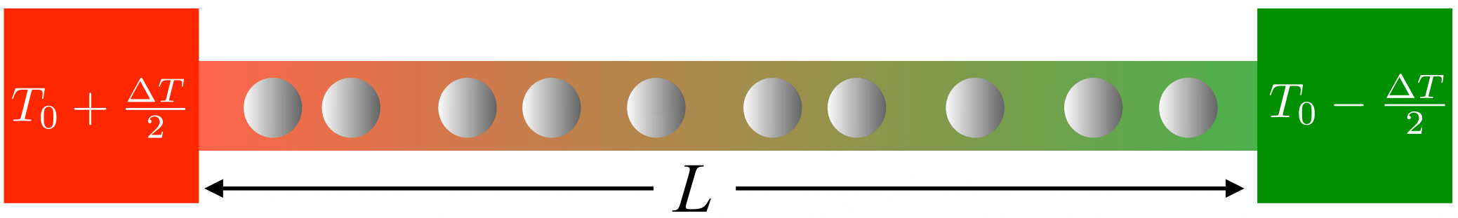
Figure 1: A gas of unit-mass particles undergoing TPCs, attached to hot and cold Maxwell heat baths at its two ends.

II Main results

Starting from the appropriate master equation, we obtain a “noisy” Boltzmann equation, which is then used to derive the NFH equations for the conserved fields with explicit expressions of the diffusion and the noise terms. The TPC model has three conserved fields, namely the particle density $\rho(x,t)$, the momentum density $\rho u$ and the energy density $\rho e$ where $u(x,t)$ and $e(x,t)$ are the average momentum and energy per particle, respectively. Applying the NFH framework to these equations, one finds that the stationary energy current asymptotically decays as $L^{-2/3}$. However, the fact that the diffusion constant can be explicitly computed for the TPC model makes it particularly appealing for studying the diffusive corrections to the leading anomalous behavior. Thus, accounting for both leading and diffusive contributions enables one to observe a crossover from one regime to the other upon varying $L$.

We find that for small $\Delta T$, the stationary energy current $J_{e}$ can be written as the sum of a diffusive (normal) part $J_{e}^{N}\sim L^{-1}$ and an anomalous part $J_{e}^{A}\sim L^{-2/3}$ :

$$J_{e}=J_{e}^{N}+J_{e}^{A}=-D\left(1+\left(\frac{L}{\ell_{c}}\right)^{1/3}\right)\frac{\Delta T}{L}$$ (1)

where $D$ is the energy diffusion coefficient and $\ell_{c}$ is the length-scale at which the crossover from diffusive to anomalous transport takes place. Explicit expressions of $D$ and $\ell_{c}$ are given in terms of the model parameters in (7) and (42) respectively. It is evident from the expression of $J_{e}$ in (1) that for $L\ll\ell_{c}$ the transport is diffusive whereas for $L\gg\ell_{c}$ it is anomalous. In fig. 2, $J_{e}$ is plotted against $L$ for a given set of the model parameters which determine the value of $D$ and $\ell_{c}$, supporting Eq (1). A collapse of the properly scaled $L$ dependence of the current curve for a large number of sets of model parameters is found in fig. 3. In this figure, it is demonstrated that for different sets of model parameters the current scaling falls either in the normal regime or in the anomalous regime. However, finding a single set of model parameters for which the crossover is evident proved to be numerically difficult.

The paper is organised as follows: We proceed by first deriving a stochastic Langevin-Boltzmann (LB) equation in Sec. III for the empirical density $f(x,p,t)$ which counts the number of particles per unit volume of the phase space around the point $(x,p)$. In the next section IV, we make an ansatz for the solution of the LB equation, which is then used to derive the stochastic hydrodynamic equations for the conserved density, momentum and energy fields. Our final aim is to compute the system size dependence of the current in NESS with the diffusive correction added to the leading anomalous contribution. This is achieved in Sec. V where, starting from the Fokker-Plank equation of the microscopic $N$ particle distribution, we establish a novel linear response theory which expresses the current in NESS as the time integral of the equilibrium current-current correlations through Green-Kubo formula. These correlations among the currents are, in turn, related to the correlations among the conserved field densities. Finally, these conserved field correlations are evaluated by using the stochastic hydrodynamic equations and extending the mode-coupling procedure to include the desired diffusive correction. As mentioned earlier, this diffusive correction allows us to study a crossover from normal to anomalous transport with increasing system size. We verify and establish this crossover through extensive numerical simulation. In Sec. VI we provide the details of our simulation procedure which is followed by our conclusion in Sec. VII.

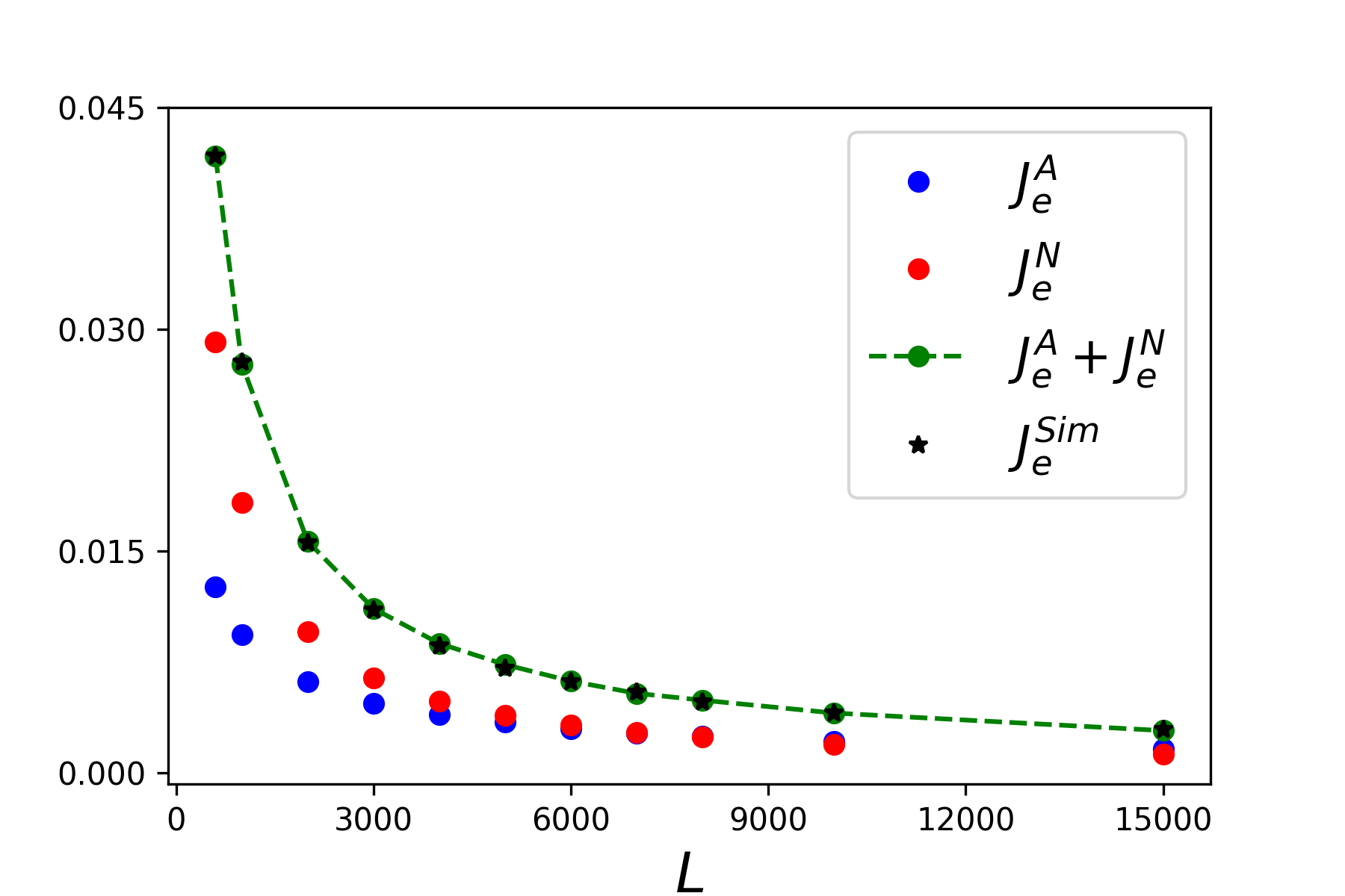
Figure 2: The stationary current $J_{e}$ as a function of system size $L$ for parameters $\rho_{0}=0.5$, $T_{0}=10$ and $\nu_{0}=0.79$. The black stars ($J_{sim}^{e}$) are direct simulation results, the blue and red points are the theoretical normal ($J_{e}^{N}\sim L^{-1}$) and anomalous ($J_{e}^{A}\sim L^{-2/3}$) currents appearing in $\left(1\right)$ and the dashed green line is their sum. We note that the temperature difference $\Delta T$ used to compute $J_{e}^{N}$ and $J_{e}^{A}$ is the bulk temperature difference, determined by taking a linear fit of the bulk temperature profile, extrapolating the linear temperature profile to the boundaries of the system and computing the difference.

III Derivation of the Langevin-Boltzmann Equation

We start by deriving the noisy Langevin-Boltzmann equation for the empirical density $f(x,p,t)$ at the phase space point $(x,p)$. This derivation follows the procedure given in Brenig and Van den Broeck (1980). We first divide the full one particle phase space $(x,p)$ into a large number of non-overlapping phase-space cells $[x,x+\text{d}x]\times[p,p+\text{d}p]$. As the particles in the TPC gas are evolving with time, the particles in neighboring phase-space cells get exchanged stochastically and thus changing the number $N_{(x,p)}(t)=f(x,p,t)\text{d}x\text{d}p$ of particles in these cells. The state of the system at time $t$ is completely specified by the set $\left\{N_{x,p}\left(t\right)\right\}$ and its evolution is described by a master equation for the joint probability distribution $P\left(\left\{N_{x,p}\right\};t\right)$

$$\partial_{t}P\left(\left\{N_{x,p}\right\};t\right)=\sum_{\left\{N^{\prime}_{x,p}\right\}}W_{\left(\left\{N^{\prime}_{x,p}\right\}\to\left\{N_{x,p}\right\}\right)}P\left(\left\{N^{\prime}_{x,p}\right\}\right)$$ (2)

where $W_{\left(\left\{N^{\prime}_{x,p}\right\}\to\left\{N_{x,p}\right\}\right)}$ is the transition rate from the state $\left\{N^{\prime}_{x,p}\right\}$ to the state $\left\{N_{x,p}\right\}$. The transition rate $W_{\left(\left\{N^{\prime}_{x,p}\right\}\to\left\{N_{x,p}\right\}\right)}$ is composed of two contributions: the first describes the drift of particles along the $x$ axis between adjacent phase-space cells, i.e $N_{x,p},N_{x+\mathbf{d}x,p}\rightarrow N_{x,p}-1,N_{x+\mathbf{d}x,p}+1$, and the second describes momenta-mixing collisions between triplets of particles occupying the same $x$ cell, i.e $N_{x,p},N_{x,p^{\prime}},N_{x,p^{\prime\prime}},N_{x,q},N_{x,q^{\prime}},N_{x,q^{\prime\prime}}\rightarrow N_{x,p}+1,N_{x,p^{\prime}}+1,N_{x,p^{\prime\prime}}+1,N_{x,q}-1,N_{x,q^{\prime}}-1,N_{x,q^{\prime\prime}}-1$. One can rewrite the above master equation as

$$\partial_{t}P\left(\left\{N_{x,p}\right\};t\right)=\left(K^{Drift}+K^{Coll}\right)P\left(\left\{N_{x,p}\right\};t\right).$$ (3)

Explicit expressions of the drift term $K^{Drift}P\left(\left\{N_{x,p}\right\}\right)$ and the collision term $K^{Coll}P\left(\left\{N_{x,p}\right\}\right)$ are given in (45) and (46) respectively. From this master equation under diffusion approximation and in the continuum limit, one obtains a Fokker-Plank equation for the empirical densities $f(x,p,t)$, which corresponds to the following Langevin-Boltzmann equation (see Appendix-A for the derivation)

$$\partial_{t}f+p\partial_{x}f=(\partial_{t}f)_{c}+\chi,$$ (4)

where $\chi\left(x,p,t\right)$ is a zero-mean Gaussian noise satisfying

$$\left\langle\chi\left(x,p,t\right)\chi\left(x^{\prime},p^{\prime},t^{\prime}\right)\right\rangle=\overline{C}\left(p,p^{\prime};f\right)\delta(x-x^{\prime})\delta(t-t^{\prime}).$$

and is detailed for the present model in Appendix-A.3. Here $\overline{C}\left(p,p^{\prime};f\right)$ is a functional of $f(x,p,t)$ and is provided explicitly in Eq. (62). Note that the noise-free part of (4) is the Boltzmann equation which provides the regular evolution of $f(x,p,t)$ whereas the noise term $\chi\left(x,p,t\right)$ describes fluctuations around this regular evolution. The collision term $(\partial_{t}f)_{c}$ on the right hand side of (4) describes three particle collisions occurring at position $x$ and is given by

$$(\partial_{t}f)_{c}=\int dp^{\prime}dp^{\prime\prime}dqdq^{\prime}dq^{\prime\prime}R({\bf p}|{\bf q})(f_{q}f_{q^{\prime}}f_{q^{\prime\prime}}-f_{p}f_{p^{\prime}}f_{p^{\prime\prime}})$$

$$\text{where},~{}~{}~{}R\left(\boldsymbol{p}|\boldsymbol{q}\right)=\gamma\delta\left(P-Q\right)\delta\left(E_{\boldsymbol{p}}-E_{\boldsymbol{q}}\right),$$ (5)

and $\gamma$ is a constant. Here, $\boldsymbol{p}\equiv\left(p,p^{\prime},p^{\prime\prime}\right)$, $f_{p}\equiv f(x,p,t)$, $P=p+p^{\prime}+p^{\prime\prime}$, $Q=q+q^{\prime}+q^{\prime\prime}$, $E_{\boldsymbol{p}}=\frac{1}{2}\left(p^{2}+p^{\prime 2}+p^{\prime\prime 2}\right)$ and similarly $E_{\boldsymbol{q}}$. The $\delta$-functions appearing in the collision kernel $R\left(\boldsymbol{p}|\boldsymbol{q}\right)$ ensure momentum and energy conservation at each collision. At this point, one needs to solve (4) for $f(x,p,t)$ along with the noise. However, this task is not straightforward as Eq. (4) is nonlinear.

IV Derivation of the stochastic hydrodynamic equations

Let us first consider the significantly simpler linearized, noise-free version of (4). This is done in a non-equilibrium setting characterized by temperature and density profiles $T\left(x\right)$ and $\rho\left(x\right)$ respectively, at constant pressure $P=\rho\left(x\right)$T$\left(x\right)$. Expanding around the local equilibrium (LE) state, Ma Ma (1983) computed the stationary $f\left(x,p\right)$, to linear order in $\partial_{x}T$, as

$$f\left(x,p\right)=\frac{\rho_{0}e^{-\frac{p^{2}}{2T_{0}}}}{\sqrt{2\pi T_{0}}}\left(1-\frac{9\sqrt{3}}{2\nu_{0}\sqrt{2T_{0}}}\varphi\left(\frac{p}{\sqrt{T_{0}}}\right)\partial_{x}T\right),$$ (6)

where $\nu_{0}=\frac{2\pi}{\sqrt{3}}\gamma\rho{}_{0}^{2}$ is the collision rate, $\rho_{0}=\frac{N}{L}$ is the average density and $\varphi\left(p\right)=\frac{p\left(p^{2}-3\right)}{\sqrt{6}}$. Using the above distribution, one finds a normal current

$$J_{e}^{N}=-D\frac{\Delta T}{L},\text{ }\text{where, }D=\frac{27\rho_{0}T_{0}}{4\nu_{0}}.$$ (7)

Note that the energy current (7) derived from the noise-free problem above does not contain the expected anomalous contribution mentioned in Eq. (1). To go beyond this simple approach, one must study the stochastic evolution of the conserved fields: $\rho\left(x,t\right)$, $\rho\left(x,t\right)u\left(x,t\right)$ and $\rho\left(x,t\right)e\left(x,t\right)$ which can be obtained from the Langevin-Boltzmann Eq (4). Assuming that the noisy evolution of the system in the non-stationary regime can be described as an evolving LE picture at HD length and time scales, we make the following ansatz for the solution of (4)

$$f\left(x,p,t\right)=\frac{\rho}{\sqrt{2\pi T}}e^{-\frac{\left(p-u\right)^{2}}{2T}}\left(1+\psi\text{ }\varphi\left(\frac{p-u}{\sqrt{T}}\right)\right)$$ (8)

where now the fields $\rho=\rho\left(x,t\right)$, $u=u\left(x,t\right)$, $T=T\left(x,t\right)$ and $\psi=\psi\left(x,t\right)$ fluctuate in time and space due to the noise $\chi$ in Eq (4). These four fields are related to the four (empirical) moments $\mu_{n}\left(x,t\right)=\int\text{d}pp^{n}f(x,p,t)$ for $n=0,1,2,3$. The evolution equations for $\mu_{n}\left(x,t\right)$ are next derived from Eqs (4) and (8), yielding the following HD equations for the three conserved fields $\rho(x,t)$, $\rho(x,t)u(x,t)$, $\rho(x,t)e(x,t)$:

$$\partial_{t}\rho+\partial_{x}\left(\rho u\right)=0$$

$$\partial_{t}\left(\rho u\right)+2\partial_{x}\left(\rho e\right)=0$$ (9)

$$\partial_{t}\left(\rho e\right)+\partial_{x}\left(\sqrt{\frac{3}{2}}\rho\psi\left(2e-u^{2}\right)^{\frac{3}{2}}+\rho u\left(3e-u^{2}\right)\right)=0,$$

and an equation for the non-conserved field $\psi(x,t)$

$$\begin{split}&\partial_{t}\rho\left(\sqrt{6}\psi g_{-}^{\frac{3}{2}}+2u\left(e+g_{-}\right)\right)+\partial_{x}\left(\sqrt{96}\rho ug_{-}^{\frac{3}{2}}\psi\right)\\ &=-2\partial_{x}\rho\left(g_{+}g_{-}+2e^{2}\right)-\frac{2\sqrt{2}\nu_{0}\rho g_{-}^{\frac{3}{2}}}{3\sqrt{3}}\psi+\sqrt{\sigma}\xi.\end{split}$$ (10)

Here $T=2e-u^{2},\text{ }g_{\pm}=2e\pm u^{2}$ and the noise term is $\xi=\int\text{d}p\text{ }p^{3}\chi(x,p,t)$ with $\sigma=8\nu_{0}\rho_{0}T_{0}^{3}/3$ (see Eq. (63)). The equations for the three conserved fields have the expected continuity form, whereas the equation for $\psi(x,t)$ does not. Also note that the currents $J_{\rho}=\rho u$ and $J_{\rho u}=\rho e$, associated with the fields $\rho$ and $\rho u$ respectively, are themselves conserved. Hence, they do not contain explicit noise terms. On the other hand, the current in the $\rho e$ equation does contain noise and dissipation terms through $\psi(x,t)$.

To proceed, we expand the fields in small fluctuations around their global equilibrium values: $\rho(x,t)\to\rho_{0}+\rho(x,t)$, $u(x,t)\to 0+u(x,t)$, $e(x,t)\to e_{0}+e(x,t)$ and $\psi(x,t)\to 0+\psi(x,t)$ (denoting the fluctuations by the same symbols) and keep only terms of linear order in fluctuations, obtaining linear fluctuating HD equations. Since the field $\psi(x,t)$ is not conserved, it evolves on a time scale of order $\sim\nu_{0}^{-1}$, much shorter than the HD time scale $\mathcal{O}(L)$ over which the conserved quantities evolve. This implies $\partial_{t}\psi=\mathcal{O}(\nu_{0}^{-2})$ and so

$$\psi\left(x,t\right)=\frac{3\sqrt{3\sigma}}{8\nu_{0}\rho_{0}\sqrt{e_{0}^{3}}}\xi-\frac{9\sqrt{3}}{2\nu_{0}\sqrt{e_{0}}}\partial_{x}e+O(\nu_{0}^{-2}),$$ (11)

where $\xi\left(x,t\right)$ is a zero-mean Gaussian white noise with $\left\langle\xi\left(x,t\right)\xi\left(x^{\prime},t^{\prime}\right)\right\rangle=\delta\left(x-x^{\prime}\right)\delta\left(t-t^{\prime}\right)$. Substituting (11) into the linearized equation for $e\left(x,t\right)$ yields

$$\rho_{0}\partial_{t}e+\partial_{x}\left(2\rho_{0}e_{0}u-2D\partial_{x}e+\sqrt{\Sigma}\xi\right)\simeq 0$$ (12)

where $\Sigma=81\sigma/(16\nu_{0}^{2})$. Note that the diffusion and the noise terms in Eq (12) satisfy the FDR

$$\frac{\Sigma}{4D}\equiv\text{var}\left[e(x,t)\right]=2e_{0}^{2}.$$ (13)

Once the diffusion and noise terms in the linearized HD equations are obtained, the NFH equations are constructed by reintroducing the previously neglected second-order conserved field fluctuations (see Eq. (68).

In the NFH theory Spohn (2014, 2016), the HD equations are written in the Lagrangian frame in which the conserved quantities are the stretch field $\ell=\rho^{-1}$, the momentum field $u$ and the energy field $e$. On the other hand, the HD equations we have derived in (9) are expressed in the Eulerian frame. By making a coordinate transformation from the Eulerian coordinates $(x,t)$ to the Lagrangian coordinates $(y,t)$ we get (see Appendix-B).

$$\partial_{t}\ell-\partial_{y}u=0$$

$$\partial_{t}u+2\partial_{y}\left(\frac{e}{\ell_{0}}-\frac{e_{0}}{\ell_{0}^{2}}\ell-\frac{e}{\ell_{0}^{2}}\ell-\frac{u^{2}}{2\ell_{0}}\right)=0$$ (14)

$$\partial_{t}e-\partial_{y}\left(\frac{2D}{\ell_{0}^{2}}\partial_{y}e-\frac{2e_{0}u}{\ell_{0}}+\frac{2u}{\ell_{0}^{2}}\left(e_{0}\ell-e\ell_{0}\right)+\sqrt{\bar{\Sigma}}\bar{\xi}\right)=0$$

where $\bar{\Sigma}=\rho_{0}\Sigma$ and $\bar{\xi}(y,t)=\xi/\sqrt{\rho_{0}}$ has zero mean and variance $\left\langle\bar{\xi}\left(y,t\right)\bar{\xi}\left(y^{\prime},t^{\prime}\right)\right\rangle=\delta\left(y-y^{\prime}\right)\delta\left(t-t^{\prime}\right)$. As before, the diffusion and noise terms are related via FDR in Eq. (13). Equations (14) are the starting-point of the NFH theory Spohn (2014, 2016). We stress that, unlike the phenomenological approach taken in the derivation of the NFH theory, the noise and diffusion terms in (14) are derived from a microscopic description of the TPC model. These equations constitute a significant part of our results.

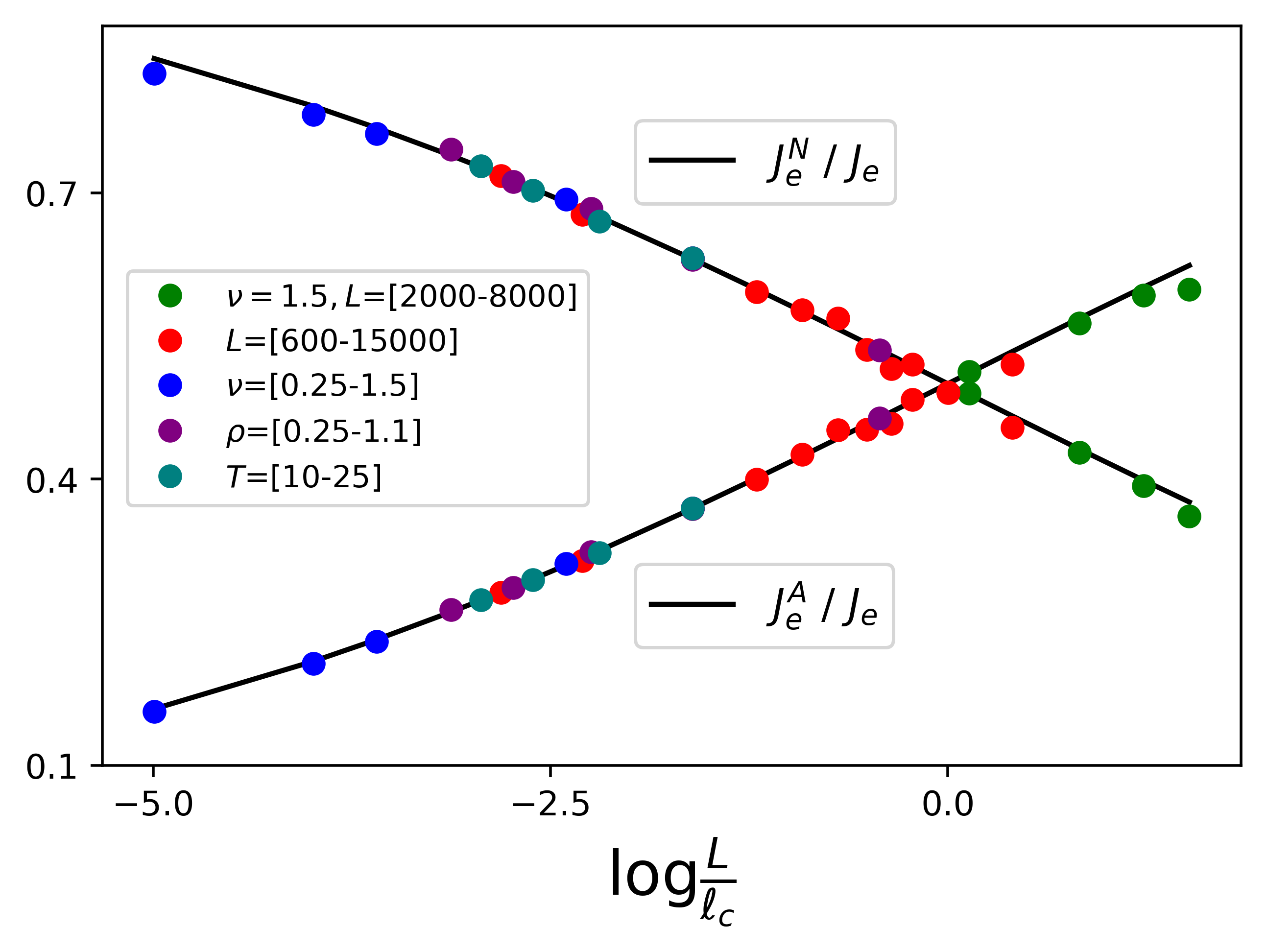
Figure 3: Data collapse of the ratios $J_{e}^{N}/J_{e}$ and $J_{e}^{A}/J_{e}$ against $u=\log\frac{L}{\ell_{c}}$ for various microscopic parameters and comparison with the collapse functions $J_{e}^{N}/J_{e}=(1+\exp(u/3))$ and $J_{e}^{A}/J_{e}=(1+\exp(-u/3))$. From (1), (7) and (42) one finds $J_{e}$ is a function of various parameters $\rho_{0}$, $T_{0}$, $\nu_{0}$, $\Delta T$ and $L$. Data points (squares and circles) are simulated by varying one parameter, keeping others fixed.

V Linear response theory

Our final aim is to obtain the $L$ dependence of the stationary energy current $J_{e}$. We start from the Fokker-Planck equation describing the evolution of the $N$-particle distribution function $P\left(\Gamma;t\right)$

$$\partial_{t}P\left(\Gamma;t\right)=\L P\left(\Gamma;t\right)$$ (15)

where the set of particle positions and momenta is denoted by $\Gamma=\left\{x_{\ell},p_{\ell}\right\}_{\ell=1}^{N}$. The FP operator $\L$ is defined by its action on a test function $g\left(\Gamma\right)$ as

$$\L g\left(\Gamma\right)=\left[-\sum_{i=1}^{N}p_{i}\partial_{x_{i}}+\L_{coll}\right]g\left(\Gamma\right)$$ (16)

with $\L_{coll}$ denoting the three-particle collision operator which conserves momentum and energy. Here, we would like to emphasise that the FP equation (15) is different from the master equation (3). The Eq. (15) describes the evolution of the joint distribution of the particles in phase space whereas the Eq. (3) describes the evolution of the probability of the occupation in regions of phase space. In this sense the Eq. (15) is a complete microscopic description whereas the Eq. (3) provides a coarse grained description which is in principle obtained from the former.

The system is driven out of equilibrium at time $t=0$ by a small temperature difference. The solution of Eq. (15) can be written as

$$P\left(\Gamma;t\right)=P_{LE}\left(\Gamma\right)+P_{dev}\left(\Gamma;t\right)$$ (17)

where $P_{LE}\left(\Gamma\right)$ is the local equilibrium distribution and $P_{dev}\left(\Gamma;t\right)$ is a deviation from it. The explicit expression for $P_{LE}\left(\Gamma\right)$ is given by

$$P_{LE}\left(\Gamma\right)=\prod_{\ell=1}^{N}\frac{\rho\left(x_{\ell}\right)}{N\sqrt{2\pi T\left(x_{\ell}\right)}}e^{-\frac{p_{\ell}^{2}}{2T\left(x_{\ell}\right)}}.$$ (18)

Substituting Eq. (17) into Eq. (15) yields

$$\partial_{t}P_{dev}\left(\Gamma;t\right)-\L P_{dev}\left(\Gamma;t\right)=\L P_{LE}\left(\Gamma\right),$$ (19)

whose formal solution is

$$P_{dev}\left(\Gamma;t\right)=\int_{0}^{t}\mathbf{d}t^{\prime}e^{\L\left(t-t^{\prime}\right)}\L P_{LE}\left(\Gamma\right),$$ (20)

with an explicit expression of $\L P_{LE}\left(\Gamma\right)$ given by.

$$\L P_{LE}\left(\Gamma\right)=-P_{LE}\left(\Gamma\right) \sum_{i=1}^{N}\left[\frac{\left(p_{i}^{3}-p_{i}T\left(x_{i}\right)\right)}{2T\left(x_{i}\right)^{2}}\right.$$

$$\left.\times\partial_{x_{i}}T\left(x_{i}\right)+p_{i}\frac{\partial_{x_{i}}\rho\left(x_{i}\right)}{\rho(x_{i})}\right].$$ (21)

It is often convenient to express the deviation $P_{dev}$ in terms of the currents generated due to the drive. For the TPC gas, one can easily define the instantaneous particle and energy density currents at position $x$ and time $t$ as

$$\begin{cases}j_{\rho}\left(x,t\right)\equiv\sum_{\ell=1}^{N}\delta\left(x_{\ell}-x\right)p_{\ell}\\ j_{e}\left(x,t\right)\equiv\sum_{\ell=1}^{N}\delta\left(x_{\ell}-x\right)\frac{p_{\ell}^{3}}{2}\end{cases}.$$ (22)

Using (22) and the gas equation of state $P=\rho\left(x\right)T\left(x\right)$ (with constant pressure $P$) in (21) gives

$$\begin{split}\L P_{LE}\left(\Gamma\right)=-&P_{LE}\left(\Gamma\right)\int_{0}^{L}\mathbf{d}x^{\prime}\frac{\partial_{x^{\prime}}T\left(x^{\prime}\right)}{T\left(x^{\prime}\right)^{2}}\\ &\times\left[j_{e}\left(x^{\prime},t\right)-\frac{3}{2}T\left(x^{\prime}\right)j_{\rho}\left(x^{\prime},t\right)\right]\end{split}$$ (23)

where the $\Gamma$ dependence of the currents is implicit in Eq. (23). Substituting Eq. (23) into Eq. (20) yields the deviation from the local-equilibrium state

$$P_{dev}\left(\Gamma;t\right)= -\int_{0}^{t}\mathbf{d}t^{\prime}e^{\L\left(t-t^{\prime}\right)}P_{LE}\left(\Gamma\right)\int_{0}^{L}\mathbf{d}x^{\prime}\frac{\partial_{x^{\prime}}T\left(x^{\prime}\right)}{T\left(x^{\prime}\right)^{2}}$$

$$\times\left[j_{\rho e}\left(x^{\prime},t^{\prime}\right)-\frac{3}{2}T\left(x^{\prime}\right)j_{\rho}\left(x^{\prime},t^{\prime}\right)\right].$$ (24)

We are now in a position to compute the deviation of the average of any observable from its value in LE. As we are interested in currents, we compute the (non-equilibrium) average particle density current and the energy density current, $J_{\rho}$ and $J_{e}$ respectively,

$$\begin{split}J_{\rho}\left(x,t\right)=&\int\text{d}\Gamma P_{dev}\left(\Gamma,t\right)j_{\rho}\left(x,t\right)\\ J_{e}\left(x,t\right)=&\int\text{d}\Gamma P_{dev}\left(\Gamma,t\right)j_{e}\left(x,t\right),\end{split}$$ (25)

in the long time limit $t\rightarrow\infty$ gives

$$J_{\rho}(x)= -\int_{0}^{t}\mathbf{d}t\int_{0}^{L}\mathbf{d}x^{\prime}\left[\left\langle j_{\rho}\left(x,t\right)j_{e}\left(x^{\prime},0\right)\right\rangle_{eq}\right.$$

$$\left.-\frac{3}{2}T\left(x^{\prime}\right)\left\langle j_{\rho}\left(x,t\right)j_{\rho}\left(x^{\prime},0\right)\right\rangle_{eq}\right]\frac{\partial_{x^{\prime}}T\left(x^{\prime}\right)}{T\left(x^{\prime}\right)^{2}}$$ (26)

$$J_{e}(x)= -\int_{0}^{\infty}\mathbf{d}t\int_{0}^{L}\mathbf{d}x^{\prime}\left[\left\langle j_{e}\left(x,t\right)j_{e}\left(x^{\prime},0\right)\right\rangle_{eq}\right.$$

$$\left.-\frac{3}{2}T\left(x^{\prime}\right)\left\langle j_{e}\left(x,t\right)j_{\rho}\left(x^{\prime},0\right)\right\rangle_{eq}\right]\frac{\partial_{x^{\prime}}T\left(x^{\prime}\right)}{T\left(x^{\prime}\right)^{2}}$$ (27)

where $\left\langle\cdot\right\rangle_{eq}$ denotes an average with respect to the local-equilibrium distribution (18).

The baths at the boundaries of our TPC gas do not allow for particle current exchange, we do not have any particle current in the steady state. Hence $J_{\rho}=0$ and applying this in (27) yields the relation

$$\int_{0}^{\infty}\mathbf{d}t\int_{0}^{L}\mathbf{d}x^{\prime}\left\langle j_{\rho}\left(x,t\right)j_{e}\left(x^{\prime},0\right)\right\rangle_{eq}\frac{\partial_{x^{\prime}}T\left(x^{\prime}\right)}{T\left(x^{\prime}\right)^{2}}$$

$$=\frac{3}{2}\int_{0}^{\infty}\mathbf{d}t\int_{0}^{L}\mathbf{d}x^{\prime}\left\langle j_{\rho}\left(x,t\right)j_{\rho}\left(x^{\prime},0\right)\right\rangle_{eq}\frac{\partial_{x^{\prime}}T\left(x^{\prime}\right)}{T\left(x^{\prime}\right)}.$$ (28)

Simplifying the expression of $J_{e}(x)$ in Eq. (27) with help of Eq. (28) gives

$$J_{e}(x)=-\int_{0}^{\infty}\mathbf{d}t\int_{0}^{L}\mathbf{d}x^{\prime}\left[\frac{1}{T\left(x^{\prime}\right)^{2}}\left\langle j_{e}\left(x,t\right)j_{e}\left(x^{\prime},0\right)\right\rangle_{eq}\right.$$

$$\left.-\frac{9}{4}\left\langle j_{\rho}\left(x,t\right)j_{\rho}\left(x^{\prime},0\right)\right\rangle_{eq}\right]\partial_{x^{\prime}}T\left(x^{\prime}\right).$$ (29)

In this context, we are only interested in the linear response thus only the leading contribution in $\partial_{x}T(x)$ is kept and $J_{e}(x)$ becomes

$$J_{e}(x)=-\frac{1}{T_{0}^{2}}\int_{0}^{\infty}\mathbf{d}t\int_{0}^{L}\mathbf{d}x^{\prime}\left[\left\langle j_{e}\left(x,t\right)j_{e}\left(x^{\prime},0\right)\right\rangle_{eq}\right.$$

$$~{}~{}~{}~{}~{}~{}~{}~{}~{}~{}~{}~{}~{}~{}\left.-\frac{9T_{0}^{2}}{4}\left\langle j_{\rho}\left(x,t\right)j_{\rho}\left(x^{\prime},0\right)\right\rangle_{eq}\right]\partial_{x^{\prime}}T\left(x^{\prime}\right).$$ (30)

To proceed, we relate the correlation functions of the currents to correlation functions of the fields. We apply the second moment sum rule for a general conserved field $a\left(x,t\right)$ and a general scaling function $g\left(x/L\right)$

$$\int dx~{}g\left(x/L\right)x^{2}\partial_{t}^{2}\langle a\left(x,t\right)a\left(0,0\right)\rangle_{eq}$$

$$~{}~{}~{}~{}\approx 2\int dx~{}g\left(x/L\right)\langle j_{a}\left(x,t\right)j_{a}\left(0,0\right)\rangle_{eq}$$ (31)

where the current $j_{a}\left(x,t\right)$ satisfies the continuity equation $\partial_{t}a\left(x,t\right)=-\partial_{x}j_{a}\left(x,t\right)$. This equation is valid in the large $L$ limit, as we have neglected terms smaller than $\mathcal{O}\left(L^{-1}\right)$. Using this relation in Eq. (30) we get

$$J_{e}\left(x\right)=-\frac{1}{T_{0}^{2}}\int_{0}^{\infty}\mathbf{d}t~{}\partial_{t}^{2}\int_{0}^{L}\mathbf{d}x^{\prime}\frac{\left(x-x^{\prime}\right)^{2}}{2}\partial_{x^{\prime}}T\left(x^{\prime}\right)$$ (32)

$$~{}~{}~{}\times\left[\left\langle\rho e\left(x,t\right)\rho e\left(x^{\prime},0\right)\right\rangle_{eq}\right.\left.-\frac{9T_{0}^{2}}{4}\left\langle\rho\left(x,t\right)\rho\left(x^{\prime},0\right)\right\rangle_{eq}\right].$$

Note that equation (32) is written in real space where $j_{e}$ is the conserved current of the energy density $\rho e$. We are interested in expressing our results in the language of the NFH theory, in which the correlation functions are derived in label space with $y\in\left[0,N\right]$. The transformation from $(x,t)$ to $(y,t)$ is given in Eq. (65)in which the fields transform as $\rho(x,t)\to\frac{1}{\ell(y,t)}$, $u(x,t)\to u(y,t)$ and $e(x,t)\to e(y,t)$. Hence, Eq. (32) in label space reads

$$J_{e}(y)=-\frac{\ell_{0}^{2}}{T_{0}^{2}}\int_{0}^{\infty}\mathbf{d}t~{}\partial_{t}^{2}\int_{0}^{N}\mathbf{d}y^{\prime}\frac{(y-y^{\prime})^{2}}{2}\partial_{y^{\prime}}T\left(y^{\prime}\right)$$ (33)

$$~{}~{}~{}\times\left[\left\langle\frac{e(y,t)}{\ell(y,t)}\frac{e(y^{\prime},0)}{\ell(y^{\prime},0)}\right\rangle_{eq}-\frac{9T_{0}^{2}}{4}\left\langle\frac{1}{\ell(y,t)}\frac{1}{\ell(y^{\prime},0)}\right\rangle_{eq}\right].$$

We now expand the fields in fluctuations around their global equilibrium values: $\ell\to\ell_{0}+\delta\ell$, $u\to 0+\delta u$ and $e\to e_{0}+\delta e$. Keeping terms up to $\mathcal{O}\left(\delta^{2}\right)$ in Eq. (33), one finds

$$\begin{split}J_{e}(y)=-&\int_{0}^{\infty}\mathbf{d}t~{}\partial_{t}^{2}\int_{0}^{N}\mathbf{d}y^{\prime}\frac{(y-y^{\prime})^{2}}{2}\partial_{y^{\prime}}T\left(y^{\prime}\right)\\ &\times\left[\frac{1}{T_{0}^{2}}\left\langle\delta e(y,t)\delta e(y^{\prime},0)\right\rangle_{eq}\right.\\ &~{}~{}~{}~{}~{}~{}-\frac{1}{\ell_{0}T_{0}}\left\langle\delta\ell(y,t)\delta e(y^{\prime},0)\right\rangle_{eq}\\ &~{}~{}~{}~{}~{}~{}~{}~{}~{}~{}\left.-\frac{2}{\ell_{0}^{2}}\left\langle\delta\ell(y,t)\delta\ell(y^{\prime},0)\right\rangle_{eq}\right].\end{split}$$ (34)

To arrive at the above expression we have used $e_{0}=T_{0}/2$ and the following properties $\langle\delta e\rangle_{eq}=\langle\delta\ell\rangle_{eq}=0$, $\langle\delta e(y,t)\delta\ell(y,t)\rangle_{eq}=\langle\delta e(y,0)\delta\ell(y,0)\rangle_{eq}=\delta(y-y^{\prime})$, $\langle\delta e(y,t)\delta\ell(y,0)\rangle_{eq}=\langle\delta\ell(y,t)\delta e(y,0)\rangle_{eq}$ and the fact that $\langle\delta e(y,t)^{2}\rangle_{eq}$ and $\langle\delta\ell(y,t)^{2}\rangle_{eq}$ are independent of $t$.

Next we compute these correlations among the conserved fields that appear in the above Eq. (34) using the evolution equations for the HD fields given in Eq. (69). In order to do so, we, at this stage, connect to the theory of NFH Spohn (2014) in which linearized evolution equations for the conserved fields $\ell\left(y,t\right),u\left(y,t\right)$ and $e\left(y,t\right)$ are first decoupled by a transformation to the eigenbasis. The eigenmodes $\phi_{\alpha}\left(y,t\right)$ ($\alpha=\pm 1,0$) are linear combinations of the fields where $\phi_{\pm 1}\left(y,t\right)$ describe two counter-propagating “sound modes” whereas $\phi_{0}\left(y,t\right)$ describes the non-propagating “heat mode”. In NFH the coupling between the sound and heat modes leads to the super-diffusive scaling of their correlation functions $f_{\alpha}\left(y,t\right)\equiv\left\langle\phi_{\alpha}\left(y,t\right)\phi_{\alpha}\left(0,0\right)\right\rangle_{eq}$ Spohn (2016, 2014) where only diagonal correlators (i.e $\left\langle\phi_{\alpha}\phi_{\beta}\right\rangle$ with $\alpha=\beta$) are observed to prevail in the long time limit $t\rightarrow\infty$. The evolution equations of these correlators are solved in the mode-coupling approximation for asymptotically long time and large distance regime, revealing their scaling form. In the TPC model, the set of $f_{\alpha}\left(y,t\right)$ are related to the conserved field correlators by

$$\begin{split}\left\langle\delta\ell\left(y,t\right)\delta\ell\left(y^{\prime},0\right)\right\rangle_{eq}=\frac{\ell_{0}^{2}}{6}&\left(f_{-1}\left(y-y^{\prime},t\right)+4f_{0}\left(y-y^{\prime},t\right)\right.\\ &~{}~{}~{}\left.+f_{+1}\left(y-y^{\prime},t\right)\right)\\ \left\langle\delta\ell\left(y,t\right)\delta e\left(y^{\prime},0\right)\right\rangle_{eq}=\frac{\ell_{0}T_{0}}{6}&\left(f_{-1}\left(y-y^{\prime},t\right)-2f_{0}\left(y-y^{\prime},t\right)\right.\\ &~{}~{}~{}\left.+f_{+1}\left(y-y^{\prime},t\right)\right)\\ \left\langle\delta e\left(y,t\right)\delta e\left(y^{\prime},0\right)\right\rangle_{eq}=\frac{T_{0}^{2}}{6}&\left(f_{-1}\left(y-y^{\prime},t\right)+f_{0}\left(y-y^{\prime},t\right)\right.\\ &~{}~{}~{}\left.+f_{+1}\left(y-y^{\prime},t\right)\right)\end{split}.$$ (35)

Note that in the above equations, the correlations among the conserved fields are calculated in global equilibrium characterised by $T_{0}$, $\ell_{0}$ and zero average momentum density, while in Eq. (34), these correlations are evaluated at local equilibrium. Since we are interested in leading orders of $\partial_{y}T(y)$, it is justified to neglect any corrections of order $\partial_{y}T(y)$ in density correlation that may be present when computed in actual local equilibrium state.

Using the correlation in Eq. (35), in Eq. (34) and simplifying one obtains

$$J_{\rho e}(y)=\frac{3}{2}\int_{0}^{\infty}\mathbf{d}t~{}\partial_{t}^{2} \int_{0}^{N}\mathbf{d}y^{\prime}\frac{\left(y-y^{\prime}\right)^{2}}{2}$$

$$\times f_{0}\left(y-y^{\prime},t\right)\partial_{y^{\prime}}T\left(y^{\prime}\right).$$ (36)

where the heat-mode correlator $f_{0}(y,t)$ is given by its Fourier transform $f_{0}(y,t)=\int\text{d}k~{}e^{2\pi iky}\hat{f}_{0}(k,t)$. The leading asymptotic scaling form

$$\hat{f}_{0}\left(k,t\right)\approx e^{-\lambda_{h}\left|k\right|^{5/3}t}$$ (37)

was obtained in Spohn (2016, 2014) with $\lambda_{h}\approx 0.3898\frac{20\pi^{8/3}}{3^{5/3}\gamma[2/3]}c$ where $c=\rho_{0}\sqrt{3T_{0}}$ is the sound velocity in the TPC model and $\gamma[x]$ denotes the Gamma function. Since the objective in Spohn (2016, 2014) was to study the leading anomalous behavior, the sub-leading diffusive contribution to (37) was not considered. Here, we are interested in the correction coming from the diffusion term. It is easy to show that by keeping the diffusive term in the mode-coupling equation for $\hat{f}_{0}\left(k,t\right)$ in Spohn (2016, 2014), the asymptotic form of $\hat{f}_{0}(k,t)$ becomes

$$\hat{f}_{0}\left(k,t\right)=e^{-t\left(\lambda_{h}\left|k\right|^{5/3}+\frac{2}{3}D\rho_{0}\left(2\pi k\right)^{2}\right)},$$ (38)

where $D=\frac{27\rho_{0}T_{0}}{4\nu_{0}}$. Inserting this form of $\hat{f}_{0}(k,t)$ into Eq. (36) and performing the remaining integrals gives

$$J_{e}\left(y\right)=\frac{3}{2} \int_{0}^{N}\mathbf{d}y^{\prime}\frac{\left(y-y^{\prime}\right)^{2}}{2}\partial_{y^{\prime}}T\left(y^{\prime}\right)\int\text{d}ke^{-2\pi ik(y-y^{\prime})}$$

$$\int_{0}^{\infty}\mathbf{d}t~{}\partial_{t}^{2}e^{-t\left(\lambda_{h}\left|k\right|^{5/3}+\frac{2}{3}D\rho_{0}\left(2\pi k\right)^{2}\right)}.$$ (39)

Using the relation $\int\text{d}k~{}e^{2\pi ik\left(y-y^{\prime}\right)}|k|^{5/3}=-\frac{\Gamma\left(\frac{8}{3}\right)}{\left(2\pi\right)^{8/3}}\left|y-y^{\prime}\right|^{-8/3}$ and simplifying, the stationary current becomes

$$J_{e}(z)=-\frac{\rho_{0}^{1/3}\sqrt{T_{0}}}{\tilde{C}L^{2/3}}\int_{0}^{1}\mathbf{d}z^{\prime}\frac{\partial_{z^{\prime}}T\left(z^{\prime}\right)}{\left|z-z^{\prime}\right|^{2/3}}-\frac{D}{L}\partial_{z}T\left(z\right)$$ (40)

where $z=y/N$, $\tilde{C}^{-1}\approx 2.75013$. Since Eq. (40) is an equation for the stationary average energy current $J_{e}(z)$, which must be independent of $z$, one can verify that there exists a temperature profile $T\left(z\right)$ such that the right hand side is also independent of $z$. Using this fact, one may integrate both sides of (40), replace the temperature profile by the scaling function $T\left(z\right)=T_{0}+\Delta T\text{ }h\left(z\right)$ and finally obtain the announced expression for the stationary energy current (Eq. (1))

$$J_{e}= -\frac{\rho_{0}^{1/3}\sqrt{T_{0}}}{C}\frac{\Delta T}{L^{2/3}}-\frac{D\Delta T}{L}$$

$$\equiv -D\left(1+\left(\frac{L}{\ell_{c}}\right)^{1/3}\right)\frac{\Delta T}{L},$$ (41)

with the crossover length $\ell_{c}$ given by

$$\ell_{c}=\left(27C\sqrt{T_{0}}/(4\nu_{0})\right)^{3}\rho_{0}^{2}.$$ (42)

and the constant $C$ by

$$\frac{1}{C}=\frac{3}{\tilde{C}}\int_{0}^{1}\mathbf{d}z^{\prime}\left[z^{\prime 1/3}+(1-z^{\prime})^{1/3}\right]\partial_{z^{\prime}}h\left(z^{\prime}\right).$$ (43)

From Eqs. (1), (7) and (42), we see that $J_{e}$ depends explicitly on the system parameters $\rho_{0}$, $T_{0}$, $\nu_{0}$, $\Delta T$ and $L$. In order to verify the theoretical expressions for $J_{e}^{A}$,$J_{e}^{N}$ and $\ell_{c}$ numerically, we plot the ratios $J_{e}^{N}/J_{e}$ and $J_{e}^{A}/J_{e}$ as a function of $u=\log(L/\ell_{c})$ where $J_{e}^{A}=J_{e}-J_{e}^{N}$ and $J_{e}^{N}$ are obtained from Eqs. (1) and (7). It is clear from (1), (7) that $J_{e}^{N}/J_{e}=(1+\exp(u/3))$ and $J_{e}^{A}/J_{e}=(1+\exp(-u/3))$. In fig. 3 we indeed see that the data for different set of parameters collapse on these scaling curves. In order to get the best collapse and matching, we have fitted the free parameter $C$ that appears in (42). Our fitted value for $C=0.83$.

VI Discussion on the simulation method

We now briefly discuss our simulation procedure. In simulations it is impossible to implement three particle collisions at a point. Instead we consider collisions between neighboring particle triplets at a constant rate $\nu_{0}$, which at high average density $\rho_{0}$ are in close proximity to each other. Consequently, momentum and energy are exchanged by particles located at different positions. This procedure introduces corrections to the diffusion and noise terms appearing in the HD equations (9) which, in turn, contributes to $J_{e}$. The correction to $J_{e}$ due to this exchange, denoted by $J_{e}^{x}$, is estimated to be $J_{e}^{x}=\frac{2\nu_{0}}{3\rho_{0}}\left(\frac{\Delta T}{L}\right)$ (see Kundu et al. (2016)). In order to minimize the contribution of exchange in the TPC model simulations, we have carefully selected parameters such that $J_{e}^{x}/J_{e}\sim 10^{-2}$, making $J_{e}^{x}$ effectively negligible. For this reason, $J_{e}^{x}$ is absent from the results shown in fig. 2 and fig. 3.

VII Conclusions

In conclusion, we have studied a one-dimensional stochastic gas model whose simple (three particle) collision mechanism conserves momentum and energy, and breaks integrability while still allowing for analytical treatment. Starting from a microscopic description, we have derived a Langevin-Boltzmann equation with a noise term describing our model and used it to derive NFH equations in which both diffusion coefficient and noise amplitude are clearly related to the microscopic model parameters and satisfy FDR. After establishing a novel linear response theory, we compute the current in NESS using the tools of mode-coupling theory. We provide an expression for the stationary energy current of the model which contains the expected leading anomalous contribution but also a normal correction to it. The crossover between normal and anomalous transport involves a typical length-scale $\ell_{c}$ of which we provide an explicit expression in terms of the microscopic parameter except for a fitting constant. We verify this crossover through extensive numerical simulations. In the present study, we consider reservoirs which prohibit a stationary particle current. Considering reservoirs which allow both particle and energy transfer could result in two stationary currents which is an interesting setup to explore. In general, boundary conditions are observed to have a noticeable effect in systems featuring anomalous transport Cividini et al. (2017); Delfini et al. (2010); Lepri and Politi (2011); Lepri et al. (2009). However, the precise effect of the boundaries in the TPC model is still unclear. Moreover, it would also be interesting to extend the present study to other models, for which the diffusion and the noise terms could be obtained.

VIII Acknowledgement

We thank H. Posch, H. van-Beijern, H. Spohn, A. Dhar and S. N. Majumdar for useful discussions. AK and JC thank the Weizmann institute of science for the hospitality received during their visit. AK also acknowledges support from DST grant under project No. ECR/2017/000634 and the support form the project 5604-2 of the Indo-French Centre for the Promotion of Advanced Research (IFCPAR).

Appendix A Derivation of the Langevin-Boltzmann equation (4)

We start from the master equation (3)

$$\partial_{t}P\left(\left\{N_{x,p}\right\};t\right)=\left(K^{Drift}+K^{Coll}\right)P\left(\left\{N_{x,p}\right\};t\right),$$ (44)

the drift term is given by

$$K^{Drift}P\left(\left\{N_{x,p}\right\}\right)=\sum_{x^{\prime},p^{\prime}}\left|p^{\prime}\right|\left[E_{x^{\prime},p^{\prime}}^{+}E_{x^{\prime}+\text{sgn}\left[p^{\prime}\right]\Delta x,p^{\prime}}^{-}-1\right]\frac{N_{x^{\prime},p^{\prime}}}{\Delta x}P\left(\left\{N_{x,p}\right\}\right)$$ (45)

and the collision term is given by

$$K^{Coll}P\left(\left\{N_{x,p}\right\}\right)=\frac{1}{3}\sum_{x}\sum_{\boldsymbol{q},\boldsymbol{p}}\tilde{\gamma}\tilde{R}_{q,q^{\prime},q^{\prime\prime}\to p,p^{\prime},p^{\prime\prime}}\left[E_{x,q}^{+}E_{x,q^{\prime}}^{+}E_{x,q^{\prime\prime}}^{+}E_{x,p}^{-}E_{x,p^{\prime}}^{-}E_{x,p^{\prime\prime}}^{-}-1\right]N_{x,q}N_{x,q^{\prime}}N_{x,q^{\prime\prime}}P\left(\left\{N_{x,p}\right\}\right)$$ (46)

where $\tilde{\gamma}$ has dimension (time)^-1 and the step operator $E_{x,p}^{\pm}$ creates/annihilates a particle at the box labeled $\left(x,p\right)$, i.e

$$E_{x,p}^{\pm 1}P\left(...,N_{x,p},...\right)=P\left(...,N_{x,p}\pm 1,...\right).$$ (47)

The notation $\sum_{\boldsymbol{q},\boldsymbol{p}}$ denotes the sums over the vectors ${\bf q}=(q,q^{\prime},q^{\prime\prime})$ and ${\bf p}=(p,p^{\prime},p^{\prime\prime})$ where the momentum components lie $\in\left(-\infty,\infty\right)$ and the kernel $\tilde{R}$ is given by

$$\tilde{R}_{q,q^{\prime},q^{\prime\prime}\to p,p^{\prime},p^{\prime\prime}}=\tilde{R}_{{\bf q}\to{\bf p}}=\delta_{p+p^{\prime}+p^{\prime\prime}-q-q^{\prime}-q^{\prime\prime}}\delta_{\frac{p^{2}+p^{\prime 2}+p^{\prime\prime 2}}{2}-\frac{q^{2}+q^{\prime 2}+q^{\prime\prime 2}}{2}}.$$ (48)

Here the $\delta$’s are Kronecker deltas. The 1/3 factor in the definition of $\overline{\gamma}$ is taken so that the resulting collision rate of the collision term in the Langevin-Boltzmann equation $\left(19\right)$ coincides with the collision rate $\gamma$, as defined in equation $\left(4\right)$.

Following Brenig and Van den Broeck (1980), we next simplify (2) by taking the continuum limit. We consider the regime where $\Delta x\Delta p$ is large enough such that there are many particles in each phase-space cell while the spatial size $\Delta x$ of each cell is much smaller than the system size $L$. Accordingly, we define the phase-space density $f_{x,p}\left(t\right)\equiv\frac{N_{x,p}\left(t\right)}{\Delta x\Delta p}$ and formulate an evolution equation for it. In this regime the step operators $E_{x,p}^{\pm}$ can be expressed by

$$E_{x,p}^{\pm}=\exp\left[\pm\frac{\partial}{\partial N_{x,p}\left(t\right)}\right]=\exp\left[\pm\frac{1}{\Delta x\Delta p}\frac{\partial}{\partial f_{x,p}\left(t\right)}\right].$$ (49)

The continuum limit is obtained by taking the cell size $\Delta x$ and $\Delta p$ to zero. In order to get the desired limit, we use the following prescriptions:

$$\begin{split}&\Delta x\sum_{x}\to\int dx,~{}~{}\Delta p\sum_{p}\to\int dp\\ &\delta_{x,y}\to\Delta x~{}\delta(x-y),~{}~{}\delta_{p,q}\to\Delta p~{}\delta(p-q)\\ &f_{x,p}\to f(x,p),~{}~{}\frac{\partial}{\partial f_{x,p}}\to\Delta x\Delta p~{}\frac{\delta}{\delta f(x,p)},\\ &\text{and},~{}~{}\tilde{R}_{{\bf q}\to{\bf p}}\to\Delta p^{3}~{}\bar{R}({\bf q}\to{\bf p}),\end{split}$$ (50)

where $f(x,p)$ is now the density function of continuous variables $x,p$. Similarly, $\bar{R}({\bf q}\to{\bf p})$ is now the collision kernel of the continuous momenta ${\bf q}$ and ${\bf p}$. In the continuum limit, the derivative $\frac{\partial}{\partial f_{x,p}}$ becomes a functional derivative $\frac{\delta}{\delta f(x,p)}$ with respect to the function $f(x,p)$.

A.1 Continuum limit of the drift term in (3)

From (45) and (49), we have

$$K^{Drift} P\left(\left\{N_{x,p}\right\}\right)$$ (51)

$$=\sum_{x^{\prime},p^{\prime}}\left|p^{\prime}\right|\Delta p~{}f_{x^{\prime},p^{\prime}}\left[\exp\left(\frac{1}{\Delta x\Delta p}\sum_{y}(\delta_{y,x^{\prime}}-\delta_{y,x^{\prime}+sgn[p^{\prime}]\Delta x^{\prime}})\frac{\partial}{\partial f_{y,p^{\prime}}}\right)-1\right]P\left(\left\{f_{x,p}\right\};t\right)$$

$$=\sum_{x^{\prime},p^{\prime}}\left|p^{\prime}\right|\Delta p~{}f_{x^{\prime},p^{\prime}}\left[\exp\left(\int dy(\delta(y-x^{\prime})-\delta(y-x^{\prime}-sgn[p^{\prime}]\Delta x^{\prime}))\frac{\delta}{\delta f(y,p^{\prime})}\right)-1\right]P\left[f(x,p);t\right]$$ (52)

$$=\int dp^{\prime}~{}p^{\prime}~{}\int dy\int dx^{\prime}\left(\frac{\partial}{\partial y}\delta(x^{\prime}-y)\right)f(x^{\prime},p^{\prime})\frac{\delta P\left[f(x,p),t\right]}{\delta f(y,p^{\prime})}+O(\Delta x)$$ (53)

$$=-\int dx\int dp\frac{\delta}{\delta f(x,p)}\left(A_{1}^{(1)}(x,p)~{}P[f(x,p);t]\right),~{}~{}\text{where}~{}~{}A_{1}^{(1)}(x,p)=-p\frac{\partial}{\partial x}f(x,p).$$ (54)

A.2 Continuum limit of the collision term in (3)

We now derive the continuum limit of the collision term. Starting from (45) and using the definition of the step operators in (49), the collision rate is expanded to second order is $\left(\Delta x\Delta p\right)^{-1}$

$$K^{Coll}P =\frac{1}{3}\sum_{x}\sum_{{\bf q},{\bf p}}\tilde{\gamma}\tilde{R}_{{\bf q}\to{\bf p}}\Delta x^{3}\Delta p^{3}f_{x,q}f_{x,q^{\prime}}f_{x,q^{\prime\prime}}$$

$$~{}~{}~{}~{}~{}~{}~{}~{}~{}~{}~{}~{}~{}\times\left[\exp\left(\frac{1}{\Delta x\Delta p}\sum_{r}\left(\delta_{r,q}+\delta_{r,q^{\prime}}+\delta_{r,q^{\prime\prime}}-\delta_{r,p}-\delta_{r,p^{\prime}}-\delta_{r,p^{\prime\prime}}\right)\frac{\partial}{\partial f_{x,r}}\right)-1\right]P(\{f_{x,p}\};t).$$ (55)

$$=\frac{1}{3}(\tilde{\gamma}\Delta x^{2})\int dx\int d{\bf q}\int d{\bf p}~{}\bar{R}({\bf q}\to{\bf p})~{}f(x,q)f(x,q^{\prime})f(x,q^{\prime\prime})\left[\exp\left(\int dr~{}\Delta(r,{\bf q,p})\frac{\delta}{\delta f(x,r)}\right)-1\right]P[f(x,p);t],$$

where

$$\Delta(r,{\bf q,p})=\delta(r-q)+\delta(r-q^{\prime})+\delta(r-q^{\prime\prime})-\delta(r-p)-\delta(r-p^{\prime})-\delta(r-p^{\prime\prime}).$$ (56)

In the $\tilde{\gamma}\to\infty$ and $\Delta x^{2}\to 0$ limit we keep $\tilde{\gamma}\Delta x^{2}=\gamma$ finite. Note that $\gamma$ has the dimension (time $\times$ density²)^-1, as in the Ma’s paper Ma (1983). Following Brenig et al. Brenig and Van den Broeck (1980), we make the diffusion approximation which amounts to expanding the exponential term in upto second order. Finally we get

$$K^{Coll}P =\frac{1}{3}\int dx\int d{\bf q}\int d{\bf p}~{}\gamma~{}\bar{R}({\bf q}\to{\bf p})~{}f(x,q)f(x,q^{\prime})f(x,q^{\prime\prime})\left[\int dr\Delta(r,{\bf q,p})\frac{\delta}{\delta f(x,r)}\right.$$

$$~{}~{}~{}~{}~{}~{}~{}~{}~{}~{}~{}~{}~{}~{}~{}~{}~{}~{}~{}~{}~{}~{}~{}\left.+\frac{1}{2}\int dr\int dr^{\prime}\Delta(r,{\bf q,p})\Delta(r^{\prime},{\bf q,p})\frac{\delta^{2}}{\delta f(x,r)\delta f(x,r^{\prime})}\right]P[f(x,p);t],$$

$$=-\int dx\int dp\frac{\delta}{\delta f(x,p)}\left(A_{1}^{(2)}(x,p)P[f(x,p);t]\right)$$

$$~{}~{}~{}~{}~{}~{}~{}~{}~{}~{}~{}~{}~{}+\frac{1}{2}\int dx\int dx^{\prime}\int dr\int dr^{\prime}\frac{\delta^{2}}{\delta f(x,r)\delta f(x,r^{\prime})}\left(A^{(2)}(x,r,x^{\prime},r^{\prime})P[f(x,p);t]\right),$$ (57)

where

$$A_{1}^{(2)}(x,p) =\int dp^{\prime}\int dp^{\prime\prime}\int dq\int dq^{\prime}\int dq^{\prime\prime}\gamma~{}\bar{R}({\bf q\to p})~{}[f(x,q)f(x,q^{\prime})f(x,q^{\prime\prime})-f(x,p)f(x,p^{\prime})f(x,p^{\prime\prime})],$$

$$A^{(2)}(x,r,x^{\prime},r^{\prime}) =\frac{\delta(x-x^{\prime})}{3}\int dp^{\prime}\int dp^{\prime\prime}\int dq\int dq^{\prime}\int dq^{\prime\prime}~{}\gamma~{}\bar{R}({\bf q\to p})f(x,q)f(x,q^{\prime})f(x,q^{\prime\prime})$$

$$~{}~{}~{}~{}~{}~{}\times\left[\delta\left(q-r\right)+\delta\left(q^{\prime}-r\right)+\delta\left(q^{\prime\prime}-r\right)-\delta\left(p-r\right)-\delta\left(p^{\prime}-r\right)-\delta\left(p^{\prime\prime}-r\right)\right]$$

$$~{}~{}~{}~{}~{}~{}\times\left[\delta\left(q-r^{\prime}\right)+\delta\left(q^{\prime}-r^{\prime}\right)+\delta\left(q^{\prime\prime}-r^{\prime}\right)-\delta\left(p-r^{\prime}\right)-\delta\left(p^{\prime}-r^{\prime}\right)-\delta\left(p^{\prime\prime}-r^{\prime}\right)\right].$$ (58)

A.3 Fokker-Plank equation for the density function $f(x,p)$

Combining the terms in equations (54) and (57), we get the following Fokker-Planck equation as the continuum limit of the master equation (3)

$$\partial_{t}P\left[\left\{f\left(x,p\right)\right\},t\right] =-\int\text{d}x\int\text{d}p\frac{\delta}{\delta f\left(x,p\right)}\left(A_{1}(x,p)P[f(x,p);t]\right)$$

$$~{}~{}~{}~{}~{}~{}~{}~{}~{}~{}~{}~{}+\frac{1}{2}\int\text{d}x\int\text{d}p\int\mathbf{d}x^{\prime}\int\text{d}p^{\prime}\frac{\delta^{2}}{\delta f\left(x,p\right)\delta f\left(x^{\prime},p^{\prime}\right)}\left(A_{2}(x,p,x^{\prime},p^{\prime})P[f(x,p);t]\right)$$ (59)

where $A_{1}(x,p)=A_{1}^{(1)}(x,p)+A_{1}^{(2)}(x,p)$ and given explicitly by

$$A_{1}(x,p)=-p\frac{\partial}{\partial x}f(x,p)+\int dp^{\prime}\int dp^{\prime\prime}\int dq\int dq^{\prime}\int dq^{\prime\prime}~{}R({\bf q\to p})~{}[f(x,q)f(x,q^{\prime})f(x,q^{\prime\prime})-f(x,p)f(x,p^{\prime})f(x,p^{\prime\prime})].$$ (60)

Here $R({\bf q\to p})\equiv R({\bf q|p})=\gamma\bar{R}({\bf q\to p})$ and $A_{2}(x,p,x^{\prime},p^{\prime})$ is given in (58). Note that the second term on the right hand side of (60) is equal to $\left(\partial_{t}f\right)_{c}$ in equation (5). The Langevin-Boltzmann equation corresponding to the Fokker Planck equation (59) can be identified and it is given by

$$\partial_{t}f\left(x,p,t\right)=-p\partial_{x}f\left(x,p,t\right)+\left(\partial_{t}f\right)_{c}\left(x,p,t\right)+\chi\left(x,p,t\right),$$ (61)

where $\chi\left(x,p,t\right)$ is a mean zero Gaussian white noise whose properties are determined by $A_{2}(x,p,x^{\prime},p^{\prime})$:

$$\langle\chi\left(x,p,t\right)\chi\left(x^{\prime},p^{\prime},t^{\prime}\right)\rangle = \delta\left(t-t^{\prime}\right)\delta\left(x-x^{\prime}\right)A_{2}(x,p,x^{\prime},p^{\prime})$$ (62)

$$= \frac{1}{3}\delta\left(t-t^{\prime}\right)\delta\left(x-x^{\prime}\right)\int\mathbf{d}p_{1}\mathbf{d}p_{2}\mathbf{d}p_{3}\mathbf{d}q_{1}\mathbf{d}q_{2}\mathbf{d}q_{3}R\left(q_{1},q_{2},q_{3}\to p_{1},p_{2},p_{3}\right)f\left(x^{\prime},q_{1}\right)f\left(x^{\prime},q_{2}\right)f\left(x^{\prime},q_{3}\right)$$

$$\times\left[\delta\left(q_{1}-p\right)+\delta\left(q_{2}-p\right)+\delta\left(q_{3}-p\right)-\delta\left(p_{1}-p\right)-\delta\left(p_{2}-p\right)-\delta\left(p_{3}-p\right)\right]$$

$$\times\left[\delta\left(q_{1}-p^{\prime}\right)+\delta\left(q_{2}-p^{\prime}\right)+\delta\left(q_{3}-p^{\prime}\right)-\delta\left(p_{1}-p^{\prime}\right)-\delta\left(p_{2}-p^{\prime}\right)-\delta\left(p_{3}-p^{\prime}\right)\right].$$

In the main text we have used this Langevin-Boltzmann equation (61) to derive equations for the first four moments (Eqs. (9) and (10) of the main text), with the noise $\chi$ appearing only in last equation as $\sqrt{\sigma}\xi\left(x,t\right)=\int\mathbf{d}pp^{3}\chi\left(x,p,t\right)$. These equations are linearized by expanding the fields in small fluctuations around their global equilibrium values. In the $\nu_{0}\gg 1$ limit, we derive Eq. (11) of the main text for $\psi\left(x,t\right)$. To compute the leading approximation of the noise amplitude $\sigma\left\langle\xi\left(x,t\right)\xi\left(x^{\prime},t\right)\right\rangle=\delta(t-t)\int\mathbf{d}pp^{3}\int\mathbf{d}p^{\prime}p^{\prime 3}A_{2}(x,p,x^{\prime},p^{\prime})$ in this limit, we replace $f\left(x,p,t\right)$ appearing in $A_{2}(x,p,x^{\prime},p^{\prime})$ by the global equilibrium one-particle distribution $f_{\mathrm{0}}\left(p\right)=\frac{\rho_{0}}{\sqrt{2\pi T_{0}}}e^{-\frac{p^{2}}{2T_{0}}}$. We denote the corresponding variance by $\sigma\left\langle\xi\left(x,t\right)\xi\left(x^{\prime},t\right)\right\rangle_{0}$ which reads

$$\sigma\langle\xi\left(x,t\right)\xi\left(x^{\prime},t^{\prime}\right)\rangle_{\mathrm{0}} = \delta\left(t-t^{\prime}\right)\delta\left(x-x^{\prime}\right)\frac{2\rho_{0}^{3}T_{0}^{3}\gamma}{\left(2\pi\right)^{3/2}}\int\mathbf{d}u\mathbf{d}u^{\prime}\mathbf{d}u^{\prime\prime}\mathbf{d}v\mathbf{d}v^{\prime}\mathbf{d}v^{\prime\prime}e^{-\frac{v^{2}+v^{\prime 2}+v^{\prime\prime 2}}{2}}$$ (63)

$$\times\delta(u+u^{\prime}+u^{\prime\prime}-v-v^{\prime}-v^{\prime\prime})\delta\left(\frac{1}{2}(u^{2}+u^{\prime 2}+u^{\prime\prime 2}-v^{2}-v^{\prime 2}-v^{\prime\prime 2})\right)\left[u^{6}+2u^{3}u^{\prime 3}-3u^{3}v^{3}\right]$$

$$= \frac{2\rho{}_{0}^{3}T{}_{0}^{3}\gamma}{3\left(2\pi\right)^{3/2}}\delta\left(t-t^{\prime}\right)\delta\left(x-x^{\prime}\right)\int_{P=-\infty}^{\infty}\text{d}P\int_{r=0}^{\infty}r\text{d}re^{-\frac{P^{2}}{6}-\frac{r^{2}}{2}}\frac{\pi^{2}r^{6}}{9}$$

$$= \frac{16\pi\gamma\rho{}_{0}^{3}T{}_{0}^{3}}{3\sqrt{3}}\delta\left(t-t^{\prime}\right)\delta\left(x-x^{\prime}\right)=\frac{8\nu_{0}\rho_{0}T_{0}^{3}}{3}\delta(t-t)\delta(x-x^{\prime}),$$

where we have used the variables defined in Ma (1983) to carry out integration. From Eq. (63) we identify the noise amplitude $\sigma\equiv\frac{8}{3}\nu_{0}\rho_{0}T_{0}^{3}$ appearing in equation (10) in the main text.

From the linearized equation for the energy density $\rho e$ in which the noise amplitude becomes $\Sigma=\left(\frac{9}{4\nu_{0}}\right)^{2}\sigma$ (see Eq. (12) of the main text), one can easily verify that the fluctuation dissipation relation is indeed satisfied. This is done by computing the variance of the energy $e=\frac{p^{2}}{2}$ using the equilibrium distribution $f_{\mathrm{0}}\left(p\right)$ which yields $\mbox{var}\left[e\right]=2e^{2}$. Since one independently has $\frac{\Sigma}{4D}=2e_{0}^{2}$, the expected result is obtained

$$\frac{\Sigma}{4D}=\mbox{var}\left[e_{0}\right]=2e_{0}^{2}.$$ (64)

Appendix B Transformation Between Eulerian (real space) to Lagrangian (label space) Coordinates

To easily apply the results of the NFH theory Spohn (2014), we change our reference frame from the “real-space” coordinates $(x,t)$, where $x\in\left[0,L\right]$, to the “label-space” coordinates $(y,t)$ in which $y\in\left[0,N\right]$ is the continuous particle label. The transformation between frames is given explicitly in Appendix 5 of Spohn (2014) as

$$\int^{x}dx^{\prime}\rho(x^{\prime},t)=y(x,t),~{}~{}\int^{y}dy^{\prime}\ell(y^{\prime},t)=x(y,t),$$ (65)

which is equivalent to

$$\begin{cases}\partial_{x}\rightarrow\frac{1}{\ell}\partial_{y}\\ \partial_{t}\rightarrow\partial_{t}-\frac{u}{\ell}\partial_{y}\end{cases},$$ (66)

where $\rho_{0}=N/L$ and the HD fields transform as

$$\begin{cases}\rho(x,t)\to\frac{1}{\ell(y,t)}\\ u(x,t)\to u(y,t)\\ e(x,t)\to e(y,t)\end{cases}$$ . (67)

Applying this transformation to the real-space HD equations (Eq. (9) in the main text with $\psi$ replaced by its linearized form $\left(10\right)$)

$$\partial_{t}\rho+\partial_{x}\left(\rho u\right)=0$$

$$\partial_{t}\left(\rho u\right)+2\partial_{x}\left(\rho e\right)=0$$ (68)

$$\partial_{t}\left(\rho e\right)+\partial_{x}\left(\rho u\left(3e-u^{2}\right)-2D\partial_{x}e+\sqrt{\Sigma}\xi\right)=0,$$

we find

$$\partial_{t}\ell-\partial_{y}u=0$$

$$\partial_{t}u+\partial_{y}\left(\frac{2e-u^{2}}{\ell}\right)=0$$ (69)

$$\partial_{t}e+\partial_{y}\left(\frac{u}{\ell}\left(2e-u^{2}\right)-\frac{2D}{\ell^{2}}\partial_{y}e+\sqrt{\overline{\Sigma}}\overline{\xi}\right)=0,$$

where $\overline{\Sigma}=\left(\frac{9}{4\nu_{0}}\right)^{2}\rho_{0}\sigma$ and the Gaussian white noise $\bar{\xi}(y,t)$ satisfies

$$\begin{cases}\langle\bar{\xi}(y,t)\rangle=0\\ \langle\bar{\xi}(y_{1},t_{1})\bar{\xi}(y_{2},t_{2})\rangle=\delta(y_{1}-y_{2})\delta(t_{1}-t_{2})\end{cases}.$$ (70)

Expanding the currents in Eqs. (69) to second order in fluctuations of the conserved fields, we obtain Eqs. (14) of the main text.

References

- Narayan and Ramaswamy (2002) O. Narayan and S. Ramaswamy, Phys. Rev. Lett. 89, 200601 (2002).
- Lepri et al. (2009) S. Lepri, C. Mejia-Monasterio, and A. Politi, Journal of Physics A: Mathematical and Theoretical 42, 025001 (2009).
- Dhar (2008) A. Dhar, Advances in Physics 57, 457 (2008).
- Lepri et al. (2003a) S. Lepri, R. Livi, and A. Politi, Physics Reports 377, 1 (2003a).
- Lepri et al. (1998) S. Lepri, R. Livi, and A. Politi, EPL (Europhysics Letters) 43, 271 (1998).
- Wang and Li (2004) J.-S. Wang and B. Li, Phys. Rev. Lett. 92, 074302 (2004).
- Lepri et al. (2003b) S. Lepri, R. Livi, and A. Politi, Phys. Rev. E 68, 067102 (2003b).
- Lepri (2016) S. Lepri, “Heat transport in low dimensions: Introduction and phenomenology,” in Thermal Transport in Low Dimensions: From Statistical Physics to Nanoscale Heat Transfer (Springer International Publishing, 2016) pp. 1–37.
- Spohn (2014) H. Spohn, Journal of Statistical Physics 154, 1191 (2014).
- van Beijeren (2012) H. van Beijeren, Physical review letters 108, 180601 (2012).
- Spohn (2016) H. Spohn, “Fluctuating hydrodynamics approach to equilibrium time correlations for anharmonic chains,” in Thermal Transport in Low Dimensions: From Statistical Physics to Nanoscale Heat Transfer (Springer International Publishing, Cham, 2016) pp. 107–158.
- Mendl and Spohn (2015) C. B. Mendl and H. Spohn, Journal of Statistical Mechanics: Theory and Experiment 2015, P03007 (2015).
- Chang et al. (2008) C. W. Chang, D. Okawa, H. Garcia, A. Majumdar, and A. Zettl, Phys. Rev. Lett. 101, 075903 (2008).
- Hsiao et al. (2013) T.-K. Hsiao, H.-K. Chang, S.-C. Liou, M.-W. Chu, S.-C. Lee, and C.-W. Chang, Nature nanotechnology 8, 534 (2013).
- Mai (2007) T. Mai, Phys. Rev. Lett. 98, 184301 (2007).
- Ma (1983) S. k. Ma, Journal of Statistical Physics 31, 107 (1983).
- Basile et al. (2006) G. Basile, C. Bernardin, and S. Olla, Physical review letters 96, 204303 (2006).
- Iubini et al. (2014) S. Iubini, A. Politi, and P. Politi, Journal of Statistical Physics 154, 1057 (2014).
- Szavits-Nossan et al. (2014) J. Szavits-Nossan, M. R. Evans, and S. N. Majumdar, Physical review letters 112, 020602 (2014).
- Brenig and Van den Broeck (1980) L. Brenig and C. Van den Broeck, Phys. Rev. A 21, 1039 (1980).
- Kundu et al. (2016) A. Kundu, O. Hirschberg, and D. Mukamel, Journal of Statistical Mechanics: Theory and Experiment 2016, 033108 (2016).
- Cividini et al. (2017) J. Cividini, A. Kundu, A. Miron, and D. Mukamel, Journal of Statistical Mechanics: Theory and Experiment 2017, 013203 (2017).
- Delfini et al. (2010) L. Delfini, S. Lepri, R. Livi, C. Mejia-Monasterio, and A. Politi, Journal of Physics A: Mathematical and Theoretical 43, 145001 (2010).
- Lepri and Politi (2011) S. Lepri and A. Politi, Physical Review E 83, 030107 (2011).