On Plans With Loops and Noise

Abstract.

In an influential paper, Levesque proposed a formal specification for analysing the correctness of program-like plans, such as conditional plans, iterative plans, and knowledge-based plans. He motivated a logical characterisation within the situation calculus that included binary sensing actions. While the characterisation does not immediately yield a practical algorithm, the specification serves as a general skeleton to explore the synthesis of program-like plans for reasonable, tractable fragments.

Increasingly, classical plan structures are being applied to stochastic environments such as robotics applications. This raises the question as to what the specification for correctness should look like, since Levesque’s account makes the assumption that sensing is exact and actions are deterministic. Building on a situation calculus theory for reasoning about degrees of belief and noise, we revisit the execution semantics of generalised plans. The specification is then used to analyse the correctness of example plans.

1. Introduction

In an influential paper, Levesque DBLP:conf/aaai/Levesque96 proposed a formal specification for analysing the correctness of program-like plans, such as conditional plans, iterative plans, and knowledge-based plans. The problem setting is this: in a world where the agent can affect changes by acting and learn about the truth of fluent values by sensing, what should a plan look like and how should we verify that it is correct? As a simple example, consider the problem of chopping down a tree of unknown thickness using a chop action that reduces its thickness by a unit. Clearly, no fixed sequence of chops would work; however, if one is able to check after each chop whether the tree still stands, then a simple iterative plan like in Figure 1 achieves the desired outcome. To analyse such plans, Levesque motivated an epistemic characterisation within the logical language of the situation calculus that included binary sensing actions. In that account, the planning task is to find a structure such that for every situation (that is, world state) considered initially possible, it leads to a final situation where the goal holds. While the characterisation does not immediately yield a practical algorithm, the specification serves as a general skeleton to explore the synthesis of program-like plans for reasonable, tractable fragments Cimatti200335 ; DBLP:conf/aips/BonetPG09 ; DBLP:conf/aips/HuG13 ; srivastava2015tractability . Moreover, recent advances in multi-agent epistemic planning DBLP:conf/aips/KominisG15 ; muise-aaai-15 are encouraging, and a formal characterisation like the one by Levesque can help relate that work to generalised planning.

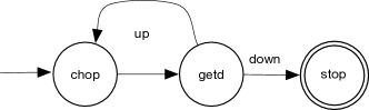
Figure 1. controller for chopping a tree of unknown non-zero thickness $d$, by means of a binary sensing action $getd$

Increasingly, classical plan structures are being applied to stochastic environments such as robotics applications mataric2007robotics . Indeed, uncertainty in the initial parameters of the planning problem is equivalent to reasoning about belief states, so robotics has long served as a motivation for generalised planning algorithms DBLP:conf/aips/BonetPG09 . Approaches such as srivastava2015tractability further allow a degree of nondeterminism in the effects of actions. This raises the question as to what the specification for correctness should look like in general, since Levesque’s account makes the assumption that sensing is exact and actions are deterministic. In fact, Levesque concludes his paper with:

“But suppose that sensing involves reading from a noisy sensor $\ldots$ how robot programs or planning could be defined in terms of this account still remains to be seen.”

To the best of our knowledge, no attempt has been made to address the issue at the level of generality of the original paper, and this is precisely our aim here. Building on a situation calculus theory for reasoning about degrees of belief and noise, our main contribution is to revisit the execution semantics of generalised plans. Concretely, beginning with the established case of exact sensing and deterministic acting, we turn to the case of exact sensing but noisy acting. We then motivate the case where both acting and sensing is noisy. We formally establish some compatibility theorems between these accounts. Finally, the specification is then used to analyse the correctness of example plans.

We reiterate that the technical thrust of this paper is limited to formal characterisations: at no point will we concern ourselves with algorithmic ideas or plan heuristics. We will mainly show how the account correctly handles changes to the state of the world as a result of noisy actions, as well as the changes to the beliefs of an agent after noisy sensing.

In this paper, there is a natural evolution of theory and formulation when compared to Levesque’s account. The original account was based on the situation calculus extended for knowledge and sensing citeulike:528170 derived from classical epistemic logic reasoning:about:knowledge . Our account is based on the situation calculus extended for probabilistic belief and noise bacchus1999171 derived from probabilistic epistemic logic bacchus1990representing ; 174658 . In principle, of course, any logical language for reasoning about actions and probabilities could have been used for the formalisation, e.g. kooi2003probabilistic . But by using the situation calculus, we can clearly explicate the generalisation from Levesque’s account, but also benefit from its first-order expressiveness, at least for axiomatising the planning domain. Moreover, to logically characterise unbounded iteration and transitive closure, we use second-order logic, as would Levesque.

Its worth remarking that while this logical machinery makes the account more involved than (say) POMDP specifications Kaelbling199899 , having a more general language is useful for contextualising involved extensions such as the handling of non-unique prior distributions. For example, in DBLP:journals/ijrr/KaelblingL13 , it is argued that when planning in highly stochastic and unknown environments, it is useful to allow a margin of error in what the values of fluents will be. This means that the planning system has to reason about multiple distributions satisfying such constraints, and as in DBLP:journals/ijrr/KaelblingL13 , the use of logical connectives allows us to express such scenarios effortlessly.

2. A Theory of Knowledge and Action

We will not go over the language ${\mathcal{L}}$ of the situation calculus in detail McCarthy:69 ; reiter2001knowledge , but simply note that it is a many-sorted dialect of predicate calculus, with sorts for actions, situations, denoting a (possibly) empty sequence of actions, and objects, for everything else. A special constant ${S_{0}}$ denotes the real world initially, and the term $do(a,s)$ denotes the situation obtained on doing $a$ in $s.$ Fluents, whose last argument is always a situation, can be used to capture changing properties. Following reiter2001knowledge , application domains are axiomatised as basic action theories, which stipulate the conditions under which actions are executable, and their affects on fluents, while embodying a monotonic solution to the frame problem. For example, for the tree chop problem, using the functional fluent $d$ to mean the thickness of the tree, we may have:

$\begin{array}[]{l}\textit{Poss}(chop(x),s)\equiv d(s)\geq x.\\[8.61108pt] d(do(a,s))=u\leavevmode\nobreak\ \equiv\\ \quad\quad\quad\quad\quad\quad\quad\quad(a=chop(x)\land d(s)=u+x)\leavevmode\nobreak\ \lor\\ \quad\quad\quad\quad\quad\quad\quad\quad(a\neq chop(x)\land d(s)=u).\end{array}$

We let $chop$ be an abbreviation for $chop(1)$. These axioms say that $chop$ is only possible when the tree’s thickness is non-zero, and that the current value of $d$ is $u$ if and only if its previous value was also $u$ and no $chop$ action occurred, or its previous value was $u+1$ and a single $chop$ action was executed.

A special binary fluent $K(s^{\prime},s)$ denotes that $s^{\prime}$ is a possible world when the agent is at $s.$ As usual, knowledge is defined as truth at accessible worlds:

$${\it Know}(\phi,s)\doteq\forall s^{\prime}.\leavevmode\nobreak\ K(s^{\prime},s)\supset\phi[s^{\prime}].$$

A modeler axiomatises the initial beliefs of the agent:

$$K({\iota},{S_{0}})\supset(1\leq d({\iota})\leq 10).$$ (1)

This is equivalently written using ${\it Know}$ and a special term $now$ to denote the current situation as:

$${\it Know}(d(now)=1\lor\ldots\lor d(now)=10,{S_{0}}).$$

The observations obtained by the agent are described using a special function ${\it SF}.$ In the tree chop problem, we may have:

$${\it SF}(a,s)=\begin{cases}{\it down}&a=getd\land d(s)=0\\ {\it up}&a=getd\land d(s)\neq 0\\ {\it 0}&\textrm{otherwise}\end{cases}$$ (2)

which says that on doing the sensing action $getd$, if the tree is still standing, the sensor returns $up$, else it would return $down.$

A fixed successor state axiom for $K$ then determines how the agent’s knowledge changes over actions:

$$\begin{array}[]{l}K(s^{\prime},do(a,s))\equiv\exists s^{\prime\prime}[K(s^{\prime\prime},s)\land s^{\prime}=do(a,s^{\prime\prime})\land Poss(a,s^{\prime\prime})\\ \hskip 71.13188pt\leavevmode\nobreak\ \land({\it SF}(a,s^{\prime\prime})={\it SF}(a,s)))]\end{array}$$

which has the effect of eliminating worlds that disagree with truth at the real world, leading to knowledge expansion.

Plans with loops

We will be interested in computable program-like plans. We consider finite state controllers, which are fairly common in the literature DBLP:conf/aips/BonetPG09 ; DBLP:conf/aips/HuG13 ; DBLP:conf/ijcai/HuL11 .

Definition .

Suppose ${\cal A}$ is a finite set of (parameterless) action terms, and ${\cal O}$ a finite set of objects, denoting observations. A finite memoryless plan ${\cal X}$ is a tuple $\la{\cal Q},{Q_{0}},{Q_{F}},\gamma,\delta\rangle$:

• ${\cal Q}$ is a finite set of control states;

• ${Q_{0}}\in{\cal Q}$ is the initial state, and ${Q_{F}}\in{\cal Q}$ the final one;

• $\gamma\in[{\cal Q}^{-}\rightarrow{\cal A}]$ is a labelling function for ${\cal Q}^{-}={\cal Q}-\left\{{Q_{F}}\right\}$;

• $\delta\in[{\cal Q}^{-}\times{\cal O}\rightarrow{\cal Q}]$ is a transition function.

Example

For Figure 1, we might have ${\cal Q}=\{{Q_{0}},Q,{Q_{F}}\},$ $\gamma({Q_{0}})=chop,\gamma(Q)=getd,\delta(Q,up)={Q_{0}},$ $\delta(Q,down)={Q_{F}},$ and $\delta({Q_{0}},1)=Q.$

Informally, we may think of applying these plans in an environment as follows: starting from ${Q_{0}}$ that advises the action $\gamma({Q_{0}})$, the environment executes that action and changes externally to return $o\in{\cal O}$. Then, internally, we reach the control state $\delta({Q_{0}},o)$ and so on, until ${Q_{F}}$. To reason about these plans in an environment enabled in the situation calculus, we need to encode the plan structure as a ${\cal L}$-sentence, and axiomatise the execution semantics over situations, for which we follow DBLP:conf/ijcai/HuL11 and define:

Definition .

Let $\mathit{\Sigma}$ be the union of the following axioms for:

1. domain closure for the control states: $(\forall q)\leavevmode\nobreak\ \{q={Q_{0}}\lor q=Q_{1}\lor\ldots\lor q=Q_{n}\lor q={Q_{F}}\};$

2. unique names axiom for the control states: $Q_{i}\neq Q_{j}\text{ \leavevmode\nobreak\ for\leavevmode\nobreak\ }i\neq j;$

3. action association: $\forall Q\in{\cal Q}^{-}$ of the form $\gamma(Q)=a$;

4. transitions: $\forall Q\in{\cal Q}^{-}$ of the form $\delta(Q,o)=Q^{\prime}$.

Definition .

We use $T^{*}(q,s,q^{\prime},s^{\prime})$ as abbreviation for $\forall T[\ldots\supset T(q,s,q^{\prime},s^{\prime})]$, where the ellipsis is the conjunction of the universal closure of:

• $T(q,s,q,s)$

• $T(q,s,q^{\prime\prime},s^{\prime\prime})\land T(q^{\prime\prime},s^{\prime\prime},q^{\prime},s^{\prime})\supset T(q,s,q^{\prime},s^{\prime})$

• $\gamma(q)=a\land Poss(a,s)\land{\it SF}(a,s)=o$
    $\land\leavevmode\nobreak\ \delta(q,o)=q^{\prime}\supset T(q,s,q^{\prime},do(a,s))$.

In English: $T^{*}$ is the reflexive transitive closure of the one-step transitions in the plan.

We are now prepared to reason about plan correctness:

Definition .

For any goal formula $\phi\in{\cal L},$ basic action theory ${\cal D},$ plan ${\cal X}$ and its encoding $\mathit{\Sigma},$ we say ${\cal X}$ is correct for $\phi$ iff

$${\cal D}\cup\mathit{\Sigma}\models\forall s.\leavevmode\nobreak\ K(s,{S_{0}})\supset\exists s^{\prime}[T^{*}({Q_{0}},s,{Q_{F}},s^{\prime})\land\phi(s^{\prime})].$$

Example

Let ${\cal D}_{dyn}$ denote the tree chop axioms, and then it is easy to see that ${\cal D}_{dyn}\cup\left\{\eqref{eq:knowledge thickness discrete},\eqref{eq exact sensing tree chop}\right\}\cup\mathit{\Sigma}$, where $\mathit{\Sigma}$ represents the encoding of Figure 1, is correct for the goal $d=0.$

3. A Theory of Probabilistic Beliefs

Our objective now is to generalise the above well-understood framework on knowledge and loopy plans to a stochastic setting. The account of knowledge, deterministic acting and exact sensing was extended by Bacchus, Halpern, and Levesque bacchus1999171 – BHL henceforth – to deal with degrees of belief in formulas, and in particular, with how degrees of belief should evolve in the presence of noisy sensing and acting, in accordance with Bayesian conditioning. The main advantage of a logical account like BHL is that it allows a specification of belief that can be partial or incomplete, in keeping with whatever information is available about the application domain. The account is based on 3 distinguished fluents: $p,l$ and $alt$. The $p$ fluent here is a numeric analogue to $K$ in that $p(s^{\prime},s)$ denotes the weight (or density) accorded to $s^{\prime}$ when the agent is at $s.$ Initial constraints about what is known can be provided as usual. For example:

$$p({\iota},{S_{0}})=\begin{cases}.1&\textrm{if }(1\leq d({\iota})\leq 10)\\ 0&\textrm{otherwise}\end{cases}$$ (3)

is saying that the tree’s thickness $d$ takes a value that is uniformly drawn from $\{1,\ldots,10\}$. We provide a definition for a belief modality ${\it Bel}$ shortly, but the above constraint can be equivalently written as:

$${\it Bel}(d(now)=1,{S_{0}})=.1$$

and so on for the other values. As argued earlier, the logical account also allows for uncertainty about the prior distribution – as needed, for example, in DBLP:journals/ijrr/KaelblingL13 – by means of expressions such as:

$${\it Bel}(d(now)=1,{S_{0}})\geq.05$$

which says that any distribution where $d$ takes a value of $1$ with a probability greater than or equal to $.05$ is a permissible one.

The $l$ fluent is used to express the likelihoods of outcomes. For example, suppose we had a sensor that would inform the agent about the numeric value of the $d$ fluent in a situation. Then an axiom of the form:

$$l(getd(z),s)={\cal N}(z;d(s),.25)$$ (4)

says that the observed value on the sensor is normally distributed around the true value, with a variance of .25. In robotics terminology thrun2005probabilistic , the sensor is said to have a Gaussian error profile.

To handle noisy actions, the idea is that if $chop(x)$ represents a chop that decrement’s the tree’s thickness by $x$ units, assume a new action type $chop(x,y)$ in that $x$ is the intended argument and $y$ is taken to be what actually happens. These are chosen by nature, and as such, out of the agent’s control. These action types are retrofitted in successor state axioms:

$$\begin{array}[]{l}d(do(a,s))=u\equiv(a=chop(x,y)\land u=d(s)-y)\leavevmode\nobreak\ \lor\\ \quad\quad\quad\quad\quad\quad\quad\quad\quad\quad(a\neq chop(x,y)\land u=d(s))\end{array}$$ (5)

says that $d$ is actually affected by the second argument.

Since the agent is assumed to not control $y,$ we use $alt$ to model the possible alternatives to an intended action:

$$alt(chop(x,y),a^{\prime},z)\equiv a^{\prime}=chop(x,z)$$ (6)

says that, for example, $chop(1,2)$ is indistinguishable from $chop(1,3)$. To suggest that some alternatives are more likely than others, an axiom like

$$l(chop(x,y),s)={\cal N}(y;x,.25)$$ (7)

then says that the actual value is normally distributed around the intended value, with a variance of .25. In robotics terminology, this is the equivalent to an action having additive Gaussian noise.

Likelihoods and alt-axioms determine the probability of successors, enabled by the following successor state axiom:

$$\begin{array}[]{l}p(s^{\prime},do(a,s))=u\,\,\equiv\\ \quad\quad\exists a^{\prime},z,s^{\prime\prime}\leavevmode\nobreak\ [\textit{alt}(a,a^{\prime},z)\land s^{\prime}=do(a^{\prime},s^{\prime\prime})\land\textit{Poss}(a^{\prime},s^{\prime\prime})\,\land\\ \quad\quad\quad\quad\quad\quad\quad\quad u=p(s^{\prime\prime},s)\times l(a^{\prime},s^{\prime\prime})]\\ \lor\,\,\lnot\exists a^{\prime},z,s^{\prime\prime}\\ \quad\quad\leavevmode\nobreak\ [\textit{alt}(a,a^{\prime},z)\land s^{\prime}=do(a^{\prime},s^{\prime\prime})\land\textit{Poss}(a^{\prime},s^{\prime\prime})\land u=0]\end{array}$$

which essentially says that if two situations $s$ and $s^{\prime}$ are considered epistemically possible, on doing $a$ at $s$, $do(a,s)$ and $do(b,s^{\prime})$ will also be considered epistemically possible, where $b$ is any $alt$-related action to $a$. Moreover, the $p$-value of $do(b,s^{\prime})$ is that of $s^{\prime}$ multiplied by the likelihood of the outcome $b$.

Putting all this together, the degree of belief in $\phi$ at $s$ is defined as the weight of worlds where $\phi$ is true:

$${\it Bel}(\phi,s)\doteq\sum_{\left\{s^{\prime}\colon\phi(s^{\prime})\right\}}p(s^{\prime},s)\leavevmode\nobreak\ \leavevmode\nobreak\ \bigg{/}\leavevmode\nobreak\ \leavevmode\nobreak\ \sum_{s^{\prime}}p(s^{\prime},s)$$

We write $K(s^{\prime},s)$ to mean $p(s^{\prime},s)>0,$ and ${\it Know}(\phi,s)\doteq{\it Bel}(\phi,s)=1.$ Finally, note that when the likelihood models are trivial, that is: $\forall a,s.\leavevmode\nobreak\ l(a,s)=1$, we are in the setting of nondeterministic but non-probabilistic acting and sensing.

4. Controllers With Noisy Acting

Our first objective will be to motivate a definition for analysing the correctness of plan structures when actions are noisy (that is, they are non-deterministic, and the actual outcome is not directly observable). We assume, for now, that sensing is exact. This then also handles the case where actions are non-deterministic but observable immediately after, by way of a sensing action to inform the planner about the outcome. As far as the syntax of the plan structure goes, we will not want it to be any different than Definition 2; however, we will need to revisit Definition 2 to internalise the noisy aspects of acting by using $alt$.

Definition .

We use $U^{*}(q,s,q^{\prime},s^{\prime})$ as abbreviation for $\forall U[\ldots\supset U(q,s,q^{\prime},s^{\prime})]$, where the ellipsis is the conjunction of the universal closure of:

• $U(q,s,q,s)$

• $U(q,s,q^{\prime\prime},s^{\prime\prime})\land U(q^{\prime\prime},s^{\prime\prime},q^{\prime},s^{\prime})\supset U(q,s,q^{\prime},s^{\prime})$

• $\gamma(q)=a\land\exists b,z\leavevmode\nobreak\ (\textit{alt}(a,b,z)\land Poss(b,s)\land{\it SF}(b,s)=o\land\delta(q,o)=q^{\prime})\supset U(q,s,q^{\prime},do(b,s))$.

The main new ingredient here over $T^{*}$, of course, is how control states transition from a situation to a successor. The reflexive transitive closure of $U$ basically says that if the controller advises $a$ and $b$ is any action that is alt-related to $a,$ we consider the transition wrt the executability and the sensing outcome of the action $b.$ The idea, then, is allow $U^{*}$ to capture the least set that accounts for all the successors of a situation where a noisy action is performed. We define:

Definition .

For any goal formula $\phi\in{\cal L},$ basic action theory ${\cal D},$ plan ${\cal X}$ and its encoding $\mathit{\Sigma},$ we say ${\cal X}$ is correct for $\phi$ iff

$${\cal D}\cup\mathit{\Sigma}\models\forall s.\leavevmode\nobreak\ K(s,{S_{0}})\supset\exists s^{\prime}[U^{*}({Q_{0}},s,{Q_{F}},s^{\prime})\land\phi(s^{\prime})].$$

It can be shown that the new semantics coincides with Levesque’s account when the action theory is noise-free: that is, alt-axioms are trivial $\forall z(\textit{alt}(a,a^{\prime},z)\equiv a=a^{\prime})$, and $l$ mimics the behavior of ${\it SF}$ in assigning 1 to situations that agree with the sensing outcome and 0 to those that disagree. Then: Suppose ${\cal D}$ is a noise-free action theory, ${\cal X}$ and $\mathit{\Sigma}$ are as above, and $\phi$ is any situation-suppressed formula not mentioning the fluent $K.$ Then, ${\cal X}$ is correct for $\phi$ in the sense of Definition 2 iff ${\cal X}$ is correct in the sense of Definition 4.

Proof.

${U^{*}}$ differs from   is only one aspect, that of alt-related actions governing the transition to a successor situation. By assumption, $\forall z(\textit{alt}(a,a^{\prime},z)\equiv a=a^{\prime})$; so Definition 2’s constraint on   coincides with Definition 4’s constraint on ${U^{*}}$.

Definition 4 only tests for a single goal-satisfying path, which is often referred to as a weak plan Cimatti200335 . A property like termination could be formalised using:

$$\begin{array}[]{l}{\cal D}\cup\mathit{\Sigma}\models\forall s.\leavevmode\nobreak\ K(s,{S_{0}})\leavevmode\nobreak\ \supset\\ \hskip 14.22636pt\forall s^{\prime}\leavevmode\nobreak\ [{U^{*}}({Q_{0}},s,q,s^{\prime})\supset\exists s^{\prime\prime}\leavevmode\nobreak\ ({U^{*}}(q,s^{\prime},{Q_{F}},s^{\prime\prime}))].\end{array}$$ (8)

It is well-known Cimatti200335 that in the absence of nondeterminism, termination is implied by the existence of a goal-satisfying path:

Proposition

Suppose ${\cal D},{\cal X}$ and $\phi$ are as above. If ${\cal X}$ is correct for $\phi$ in the sense of Definition 2 then (8) holds.

Example

Imagine a tree chop problem with noise-free sensing (i.e., let ${\it SF}$ work as in (2)), but with noisy actions. Let $chop\in{\cal A}$ correspond to the ${\cal L}$-action $chop(1,1)$, with

$$l(chop(x,y),s)=\begin{cases}.9&\textrm{if }x=y\\ .1&\textrm{if }y=0\\ 0&\textrm{otherwise}\end{cases}$$ (9)

That is, the chop action does nothing with a small probability. Letting the initial theory be a $p$-based axiom for (1), we see that the plan from Figure 1 is correct in the sense of Definition 4, and it is also a terminating plan, because regardless of how many times the action fails, there is clearly one execution path, that of the appropriate number of chops always succeeding, which stops after enabling the goal.

While Definition 4 looks at every non-zero initial world, weaker specifications are possibile still. For example:

$${\cal D}\cup\mathit{\Sigma}\models\forall s.\leavevmode\nobreak\ p(s,{S_{0}})>\kappa\supset\exists s^{\prime}[U^{*}({Q_{0}},s,{Q_{F}},s^{\prime})\land\phi(s^{\prime})]$$ (‡)

looks at worlds with weights $>\kappa$ whereas

$${\cal D}\cup\mathit{\Sigma}\models{\it Bel}(\exists s^{\prime}[U^{*}({Q_{0}},now,{Q_{F}},s^{\prime})\land\phi(s^{\prime})],{S_{0}})\geq\kappa \sharp$$ ()

says that the sum (or integral) of initial worlds where there is a weak plan is $\geq\kappa.$ Of course, since $K(s^{\prime},s)$ is an abbreviation for $p(s^{\prime},s)>0$, and ${\it Know}(\phi,s)\doteq{\it Bel}(\phi,s)=1$, we have:

Proposition

Definition 4 is equivalent to (${\ddagger}$) for $\kappa=0$, and it is equivalent to ($\sharp$) for $\kappa=1$.

Example

Imagine a tree chop problem with two types of trees, wooden ones and metal ones; the chop action has no effect on a metal tree DBLP:conf/kr/SardinaGLL06 . Suppose we have 3 worlds: the first with a wooden tree of thickness 1 and weight .4, the second with a wooden tree of thickness 2 and weight .4, and the third with a metal tree of arbitrary non-zero thickness with weight .2. If the goal is $d=0,$ and the plan is the one from Figure 1, then $({\ddagger})$ holds for (say) $\kappa=.3$ and $(\sharp)$ holds for (say) $\kappa=.7.$

We do not think that there is one preferred definition for correctness. While Definition 4 attempts correctness in the sense of Cimatti200335 , planning for likely states, as in $({\ddagger})$, is very common in robotics when exploring large biased search spaces doi:10.1177/0278364904045471 ; Knepper2017 .

5. Incorporating Noisy Sensors

Accounts like Definition 4 and ($\sharp$) capture nondeterministic acting when the outcome of the action is immediately observable. In applications such as robotics, sensing is often noisy. Similar to contingent planning DBLP:conf/aips/BonetG00 ; petrick2004extending ; muise-aaai-15 , we will now motivate a semantics of plan execution over belief states.

To review the setting informally, consider a noise-free tree chop problem instantiated by (1). Although the agent believes that $d\in\left\{1,\ldots,10\right\}$, in the real world ${S_{0}},$ the tree has a fixed thickness, say 2. In this case, the controller discussed previously will advise two chop actions, which will be executed in each of the possible worlds, including ${S_{0}}.$ At this point, a noise-free sensor returns $down,$ and so, the agent will come to believe that the tree is down. Implicitly, all the worlds other than ${S_{0}}$ considered possible initially will be discarded, as they are no longer compatible with the sensing results. (For example, the world in which $d=1$ will be discarded after the sensor says that the tree is still standing on doing a chop action, because that is clearly not possible in such a world.) However, a noisy sensor might return a $down$ despite the tree still standing. The point, then, is that the sensor’s error profile will inform the agent how likely it is that a $down$ is observed when the tree still stands, and based on that, subsequent actions can be taken until it is believed that the tree is no longer standing.

To formalise this intuition, we will need to address two technical issues. First, observe that the account of ${\it Bel}$ from BHL bacchus1999171 makes no mention of sensing functions, and in this sense, the language is only geared for projection. That is, we can infer the value of ${\it Bel}(d\leq 4,do(getd(3),{S_{0}}))$ where we explicitly provide the sensor reading, but it is ill-formed in the language to reason about beliefs after $getd$ sans argument that is determined only at run time. Moreover, as discussed above, the external feedback (e.g. number reported on a sensor) will only be an estimate of the true property when we turn to noisy sensors.

The solution to this issue by BHL was to define programs for sensing actions: for example, a sensor was defined as $\pi y.\leavevmode\nobreak\ getd(y)$, the latter being a GOLOG program reiter2001knowledge that non-deterministically chooses the argument for the sensing action. In Belle:2015ab , a slightly simpler technical device was introduced where $getd$ also stood for a program, but the semantics of program execution, which is defined over action sequences, incorporates run-time sensor readings. Neither of these solutions is appropriate for us, because: (a) we would like to avoid the complexity of defining GOLOG programs; and (b) we would like the new definition to be compatible with our previous accounts of plan execution, enabled via the ${\it SF}$ function. We achieve this by considering a runtime sensing outcome function $\Pi\colon{\cal A}^{*}\rightarrow{\cal O}$. Recall that in the situation calculus, situations are not states, and the initial situation corresponds to the setting where the agent has not executed any action. In a way, $\Pi$ is an analogue to usual definitions of observation functions that map states to observations in that it responds to an action history. Then, we use ${\it SF}$ to refer to runtime readings as follows:

$$\begin{array}[]{l}{\it SF}(a,do(a_{k},do(\ldots,do(a_{1},{\iota})\ldots)))=\Pi(a_{1},\ldots,a_{k},a).\end{array}$$

With this machinery, we can use ${\it SF}$ as usual in the plan execution semantics. We can then introduce parameterless sensing actions like $getd$ whose likelihood is now defined to mimic (4) as follows:

$$l(getd,s)={\cal N}({\it SF}(getd,s);d(s),1).$$ (10)

The second technical issue is to interpret execution paths over belief states, but while referencing the real world to test for sensing outcomes. That is, starting from a control state (from the plan structure) and the agent’s beliefs, we will need to define how a new control state is reached with an updated set of beliefs. So, we will need to “reify” beliefs in formulas: for any ground situation term $s$, we introduce a new term $\overline{s}$ to be used with formulas in that we write $\phi(\overline{s})$ to mean $\forall s^{\prime}.\leavevmode\nobreak\ K(s^{\prime},s)\supset\phi(s^{\prime}).$ We will often use two such terms in a predicate for one-step transitions: $V(t,\overline{s},t^{\prime},\overline{s}^{\prime})$ can be first expanded to $\forall s^{*}.\leavevmode\nobreak\ K(s^{*},s)\supset V(t,s^{*},t^{\prime},\overline{s}^{\prime})$, which then expands to $\forall s^{*},s^{+}.\leavevmode\nobreak\ [K(s^{*},s)\land K(s^{+},s^{\prime})]\supset V(t,s^{*},t^{\prime},s^{+})$. Recall that the $K$ fluent was assumed to be an equivalence relation, and so, roughly speaking, $V(t,\overline{s},t^{\prime},\overline{do(a,s)})$ can be seen as saying that starting from $t$ and the belief state given by the situation $s$ (that is, all $K$-related situations from $s$), we perform a transition to $t^{\prime}$ and the belief state given by $do(a,s)$. Formally, we define:

Definition .

We use $V^{*}(q,\overline{s},q^{\prime},\overline{s^{\prime}})$ as abbreviation for $\forall V[\ldots\supset V(q,\overline{s},q^{\prime},\overline{s^{\prime}})]$, where the ellipsis is the conjunction of the universal closure of:

• $V(q,\overline{s},q,\overline{s})$

• $V(q,\overline{s},q^{\prime\prime},\overline{s^{\prime\prime}})\land V(q^{\prime\prime},\overline{s^{\prime\prime}},q^{\prime},\overline{s^{\prime}})\supset V(q,\overline{s},q^{\prime},\overline{s^{\prime}})$

• $\gamma(q)=a\land Poss(a,\overline{s})\land{\it SF}(a,s)=o$
    $\land\leavevmode\nobreak\ \delta(q,o)=q^{\prime}\supset V(q,\overline{s},q^{\prime},\overline{do(a,s)})$.

The one-step transition is based on the controller advising $a,$ this action being executable at all accessible worlds, and the sensing function returning $o$ for $a$ at $s$, which is taken to be the real world. Most significantly, observe that $\phi(\overline{do(a,s)})$, by means of $p$’s successor state axiom, would implicitly account for all the alt-related actions to $a.$

With this, we are prepared to reason about correctness:

Definition .

For any goal formula $\phi\in{\cal L},$ ${\cal D},$ ${\cal X}$ and its encoding $\mathit{\Sigma},$ we say ${\cal X}$ is epistemically correct for $\phi$ iff

$${\cal D}\cup\mathit{\Sigma}\models\forall s.\leavevmode\nobreak\ K(s,{S_{0}})\supset\exists s^{\prime}\leavevmode\nobreak\ [V^{*}({Q_{0}},\overline{s},{Q_{F}},\overline{s^{\prime}})\land\phi(\overline{s^{\prime}})]$$

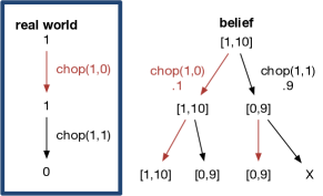
Figure 2. execution path for the tree chop problem with exact sensors against the controller from Figure 1

Before turning to the case of noisy sensors, let us revisit the tree chop problem with noisy acting and exact sensing to better understand how belief state transitions work.

Example

Let ${\cal D}$ be an action theory built from (3), (6), and the likelihood axiom (9). Suppose the sensor works as follows:

$$l(getd,s)=\begin{cases}1&{\it SF}(getd,s)=down\land d=0\\ 1&{\it SF}(getd,s)=up\land d>0\\ 0&\textrm{otherwise}\end{cases}$$ (11)

It is noise-free. Finally, suppose our goal is ${\it Bel}(d<10,now)>.9$.

A plan that is epistemically correct for this goal is given in Figure 2. We only argue for the initial world ${S_{0}}.$ It also depicts a possible execution path of the plan using $V^{*}$. Let us suppose $d({S_{0}})=1.$ The first action advised by the controller is $chop,$ and suppose the action instantiates as $chop(1,0)$. Then $d(do(chop(1,0),{S_{0}}))=1;$ so its still standing, and also, the agent accords a belief of .9 to $[0,9]$ that corresponds to a successful move, and a belief of .1 to its failure. The noise-free sensor naturally returns up. The controller advises $chop$ again, and suppose this time, the action instantiates as $chop(1,1)$.

Incidentally, even without a sensor reading, the degree of belief in $d<10$ is $>.9$ because the only branch that still entertains $d$ retaining a value of 10 is that of both chop actions failing, with a likelihood of $.1\times.1$. In any case, the controller advises a sensing action, which would return down, and so the plan terminates for $\alpha=[chop(1,0)\cdot getd\cdot chop(1,1)\cdot getd]$ with ${\it Know}({\it Bel}(d<10,now)>.9,do(\alpha,{S_{0}})).$

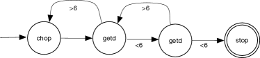
Figure 3. a controller for chopping the tree with noisy sensing

Example

Consider the tree chop problem with noisy sensors and effectors. Suppose the initial theory and alt-axioms are (3) and (6) as before, but the likelihoods for the effector is given by (7) and that for the sensor is given by (4). Finally, suppose our goal is ${\it Bel}(d\leq 5,now)>.8$.

A plan that is epistemically correct for the goal is given in Figure 3 wrt observed values of 5.5, 4.5 and 3.9. We only argue for ${S_{0}}$. Assume also that $\{<6,>6\}\in{\cal O}$ and that the numeric values obtained from the sensor map to these binary outcomes.

Here, the controller advises $chop$, after which the belief in $\psi=d\leq 5$ is $>.5.$ This is because the likelihood of the action succeeding is more than it failing, and given the prior in $d\leq 5$ is .5, the posterior should be clearly greater than $.5$. Suppose now the sensed value is 5.5. The belief in $\psi$ drops to $<.5$. The controller advises another $chop$, at which point the belief in $\psi$ increases to $>.5.$ Next, we observe a reading of 4.5 followed by 3.9. The controller terminates. On termination, it can be verified that the robot knows that the degree of belief in $\psi$ is $>.8$.

In a noise-free setting, our definition of an epistemically correct plan is downward compatible with Definition 2 (and thus, Definition 4):

Suppose ${\cal D}$ is a noise-free action theory, ${\cal X},\mathit{\Sigma}$ as above, and $\phi$ is any formula not mentioning $K.$ If ${\cal X}$ is epistemically correct for $\phi,$ then it is correct for $\phi$ in the sense of Definition 2.

Proof.

Suppose ${\cal X}$ is epistemically correct but not correct. Then there is some $s$ such that $K(s,{S_{0}})$ and $\neg\exists s^{\prime\prime}\thinspace({Q_{0}},s,{Q_{F}},s^{\prime\prime})\land\phi(s^{\prime\prime}).$ By assumption, ${V^{*}}({Q_{0}},\overline{s},{Q_{F}},\overline{s^{\prime}})\land\phi(\overline{s^{\prime}})$ for some $s^{\prime}$. Thinking of $\langle$control states, situations$\rangle$ are “nodes” in an execution path, the definition of ${V^{*}}$ is the least set of pairs of nodes containing: $\langle{Q_{0}},t\rangle$ for all situation terms $t$ such that $K(t,s)$, which includes $s$ because $K$ is assumed to be an equivalence relation; $\la q,do(a_{1},t)\rangle$ for all situation terms $t$ such that $K(t,s)$ provided ${Q_{0}}$ advises $a_{1}$, it is executable at every $t$ and the sensing function returns $o$ for $a_{1}$ at $s$ and $\delta({Q_{0}},o)=q$; and so on. By assumption, ${V^{*}}$ contains as node $\la{Q_{F}},s^{\prime}\rangle$ for $s^{\prime}=do(a_{1}\cdots a_{k},s)$. But, by the definition of $\thinspace,$ it follows that $\thinspace({Q_{0}},s,{Q_{F}},s^{\prime}).$ Moreover, since $\phi(\overline{s^{\prime}})$ and $K$ is reflexive, $\phi(s^{\prime})$. Contradiction.

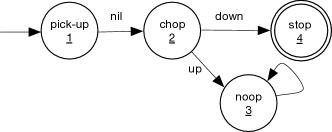
Figure 4. a problematic controller

In general, in the presence of noise, as one would expect, epistemic correctness diverges from correctness criteria based on plan evaluation at initial worlds. For example, we have:

Suppose ${\cal D}$ is any action theory, ${\cal X},\mathit{\Sigma}$ as above, and $\phi$ is any formula not mentioning $K.$ If ${\cal X}$ is epistemically correct for $\phi,$ then it does not follow that ${\cal X}$ satisfies (8).

Proof.

To prove this result, it suffices to provide a (possibly unwise) controller that is epistemically correct, but does not satisfy (8). Consider the tree chop problem for a tree of unit thickness, but with an additional action for picking up a saw. Suppose there is only a single initial world ${S_{0}},$ and $\forall a,s(Poss(a,s)\equiv\mbox{{\it true}}).$ Suppose the pick-up can fail, that is, suppose $alt(pickup,b,z)\equiv b=noop$, where $noop$ is the action of doing nothing. Suppose neither of these actions provide the agent with any meaningful sensing result: that is, $\forall s\leavevmode\nobreak\ {\it SF}(pickup,s)={\it SF}(noop,s)=nil$. Imagine a controller like in Figure 4, where the control states are designated by numbers. (That is, $q_{1}$ is the control state advising $pickup$ and $q_{4}$ is terminating state.) Initially, the controller advises $pickup$, leading to two successor situations: $do(pickup,{S_{0}})$ and $do(noop,{S_{0}})$. By way of the definition of ${\it SF}$ and $Poss$ for these actions, we have ${V^{*}}(q_{1},\overline{{S_{0}}},q_{2},\overline{do(pickup,{S_{0}})})$, ${U^{*}}(q_{1},{S_{0}},q_{2},do(pickup,{S_{0}}))$ and ${U^{*}}(q_{1},{S_{0}},q_{2},do(noop,{S_{0}}))$. Suppose now ${\it SF}(chop,do(pickup,{S_{0}}))=down$ and so we have
${V^{*}}(q_{1},\overline{{S_{0}}},q_{4},\overline{do(pickup\cdot chop,{S_{0}})})$, and by construction, $[d(now)=0](\overline{do(pickup\cdot chop,{S_{0}})}).$ However, suppose ${\it SF}(chop,do(noop,{S_{0}}))=up.$ Then we have ${U^{*}}(q_{1},{S_{0}},q_{3},do(noop\cdot chop,{S_{0}}))$, which will not terminate.

The intuitive reason is that the termination conditions defined over ${U^{*}}$ respond to sensing results along every execution path, whereas ${V^{*}}$ only responds to the sensing outcomes for the path of advised actions from an initial world and how belief changes with it. This can be seen to be not surprising: among other things, the much stronger (8) is not needed because incompatible worlds will get discarded after sensing.

Let us conclude the section with two remarks. First, as mentioned earlier, the definition of $V^{*}$ does not look very different from the semantics of noise-free belief-based planning, and this is good news: if the space of belief states is designed carefully to account for noise, algorithms for noise-free generalised planning may carry over to the stochastic case. Second, note that $V^{*}$ was defined to include an explicit reference to sensing outcomes from the environment, which is external to the agent. A result in DBLP:conf/kr/SardinaGLL06 shows that it is not possible to realise that we are making progress towards the goal without such a construction in belief-based planning.

6. Discussion and Conclusions

Generalising plans has been of interest since the early days of planning fikes1972learning . Algorithmic proposals to synthesise plans that generalise varied widely in methodology, ranging from interactive theorem proving DBLP:conf/aips/StephanB96 to learning from examples winner07_loop . The convergence of these approaches to synthesise plans that solve multiple problem instances is a recent effort DBLP:conf/aaai/BonetPG10 ; siddthesis ; levesque2005planning ; DBLP:conf/ijcai/HuL11 ; DBLP:conf/aips/HuG13 . We refer interested readers to siddthesis for a comprehensive list of references, and srivastava2015tractability ; DBLP:conf/ijcai/BonetGGR17 for recent advances on handling nondeterminism. Outside of Levesque’s account on the correctness of program-like plans as an epistemic formulation, there are numerous variants DBLP:journals/ai/LinD98 ; Cimatti200335 ; Belle:2016ab ; srivastava2015tractability ; DBLP:conf/ijcai/BonetGGR17 . The semantics $U^{*}$ extended Levesque’s $T^{*}$ to handle noisy acting, and $V^{*}$ further extends that to noisy sensing, thereby obtaining a full generalisation of the formulation to handle nondeterminism.

Belief-based planning, which we touch upon, is widely studied, e.g., DBLP:conf/aips/BonetG00 , and the usual approach is to formulate a nondeterministic (conformant) planning problem that treats belief states as first-class citizens. Our definition of ${V^{*}}$ can be seen as a formalisation of this semantics against a logic of probabilistic belief and action. In that regard, the motivation behind this work is close in spirit to knowledge-based programs DBLP:journals/tocl/Reiter01 ; DBLP:journals/sLogica/LesperanceLLS00 and its stochastic extension Belle:2015ab . These are formulated using the situation calculus and the high-level programming language GOLOG, but, of course, variant languages are also popular for developing such planning accounts thielscher:ICAART10 . At the outset, there are significant reasons to develop a semantics customised to memoryless plans, as we argue below. Moreover, since there are a number of generalised planning algorithms that synthesise loopy plans DBLP:conf/aips/HuG13 , an execution semantics tailored to that representation is useful to understand how those algorithms can be applied to domains with noise.

Let us begin by observing that memoryless plans can be easily encoded as GOLOG programs consisting of atomic physical actions and branches based on sensing outcomes. In general, given a program $\delta$, one is interested in showing that

$${\cal D}\cup\Theta\models Do(\delta,{S_{0}},do(\sigma,{S_{0}}))$$

where $\Theta$ encodes the single-step transition semantics of $\delta$, and $\sigma$ is a ground sequence of actions such that $\delta$ terminates in $do(\sigma,{S_{0}})$. The key feature of knowledge-based programs is that $\delta$ can mention ${\it Know}$, and the probabilistic belief operator ${\it Bel}$ in Belle:2015ab . Nonetheless, note that if $\delta$ does not mention ${\it Bel}$, the entailment criteria above is weaker than Definition 2 as it only looks at ${S_{0}}$. But if it mentions the ${\it Bel}$ operator, then it seems closer to Definition 5, but at the cost of a more cumbersome plan structure: $\delta$ can have unbounded memory (via while loops), can refer to complicated state properties, and is subjective, whereas Definition 5 is defined for memoryless plans built purely from a finite set of atomic actions.

So, in the current paper, the end result is an account of correctness with widely-studied loopy plan structures, which eschews the complications of GOLOG but is able to achieve almost as much. Naturally, then, relating knowledge-based programs and loopy plans (in belief-based settings) is likely to be of considerable theoretical interest, as would a closer study of the two execution semantics. (Cf. also DBLP:journals/ai/LinD98 on memoryless structures being effective, and DBLP:journals/sLogica/LesperanceLLS00 on knowing how to execute GOLOG programs.)

Despite focusing on probabilities and nondeterminism, this paper has established no connection to the large body of work on Markov decision processes puterman . Mostly, decision-theoretic planning frameworks are characterised in terms of optimality criteria against expected rewards, often enabled via dynamic programming, while we have treated goals as arbitrary formulas that are to be satisfied, as would symbolic planning frameworks such as Cimatti200335 . Nonetheless, one can imagine ways of recasting expected rewards in terms of goal satisfaction or vice versa series/synthesis/2013Geffner , and that is arguably worth doing in the context of this paper so as to relate to efforts such as poupart2004bounded . Interestingly, recent robotics planners such as DBLP:journals/ijrr/KaelblingL13 eschews a planning paradigm that advises actions for every belief state, as one would in partially observable Markov decision processes, and instead resorts to a scheme that computes plans for a designated initial belief state, as in belief-based planning. Moreover, as mentioned before, ultimately the goal here was to generalise Levesque’s account and to provide a rigorous foundation for extensions such as the handling of non-unique prior distributions.

As a final remark, like in Levesque’s original formulation, one can motivate a generic planning procedure as follows:

• input: $\phi,$ $E^{*}\in\left\{\thinspace,{U^{*}},{V^{*}}\right\},\Delta$ is a correctness criteria

• repeat with ${\cal X}\in$ FINITE STATE CONTROLLERS

• if ${\cal D}\cup\mathit{\Sigma}\models\forall s.\leavevmode\nobreak\ K(s,{S_{0}})\supset\Delta(E^{*},\phi,s)$ then return ${\cal X}$

Naturally, we do not expect to use a full-blown logical framework for planning, nor do we expect planners to actually use such a procedure in practise. Languages like the ones in Sanner:2010fk ; DBLP:journals/ijrr/KaelblingL13 seem entirely reasonable. It is also conceivable that existing algorithms for generalised planning, such as bounded AND/OR searches, can be adapted for stochastic settings, as argued earlier, possibly by leveraging abstraction techniques srivastava2015tractability ; DBLP:conf/ijcai/BonetGGR17 . We hope this paper is also useful for approaching and resolving that line of inquiry.

References

- [1] H. J. Levesque. What is planning in the presence of sensing? In Proc. AAAI / IAAI, pages 1139–1146, 1996.
- [2] A. Cimatti, M. Pistore, M. Roveri, and P. Traverso. Weak, strong, and strong cyclic planning via symbolic model checking. Artificial Intelligence, 147(1–2):35 – 84, 2003.
- [3] B. Bonet, H. Palacios, and H. Geffner. Automatic derivation of memoryless policies and finite-state controllers using classical planners. In ICAPS, 2009.
- [4] Y. Hu and G. De Giacomo. A generic technique for synthesizing bounded finite-state controllers. In ICAPS, 2013.
- [5] S. Srivastava, S. Zilberstein, A. Gupta, P. Abbeel, and S. Russell. Tractability of planning with loops. In AAAI, 2015.
- [6] F. Kominis and H. Geffner. Beliefs in multiagent planning: From one agent to many. In ICAPS, pages 147–155, 2015.
- [7] C. Muise, V. Belle, P. Felli, S. McIlraith, T. Miller, A. Pearce, and L. Sonenberg. Planning over multi-agent epistemic states: A classical planning approach. In Proc. AAAI, 2015.
- [8] M. J. Matarić. The robotics primer. Mit Press, 2007.
- [9] R. B. Scherl and H. J. Levesque. Knowledge, action, and the frame problem. Artificial Intelligence, 144(1-2):1–39, 2003.
- [10] R. Fagin, J. Y. Halpern, Y. Moses, and M. Y. Vardi. Reasoning About Knowledge. MIT Press, 1995.
- [11] F. Bacchus, J. Y. Halpern, and H. J. Levesque. Reasoning about noisy sensors and effectors in the situation calculus. Artificial Intelligence, 111(1–2):171 – 208, 1999.
- [12] F. Bacchus. Representing and Reasoning with Probabilistic Knowledge. MIT Press, 1990.
- [13] R. Fagin and J. Y. Halpern. Reasoning about knowledge and probability. J. ACM, 41(2):340–367, 1994.
- [14] B.P. Kooi. Probabilistic dynamic epistemic logic. Journal of Logic, Language and Information, 12(4):381–408, 2003.
- [15] L. P. Kaelbling, M. L. Littman, and A. R. Cassandra. Planning and acting in partially observable stochastic domains. Artificial Intelligence, 101(1–2):99 – 134, 1998.
- [16] L. P. Kaelbling and T. Lozano-Pérez. Integrated task and motion planning in belief space. I. J. Robotic Res., 32(9-10):1194–1227, 2013.
- [17] J. McCarthy and P. J. Hayes. Some philosophical problems from the standpoint of artificial intelligence. In Machine Intelligence, pages 463–502, 1969.
- [18] R. Reiter. Knowledge in action: logical foundations for specifying and implementing dynamical systems. MIT Press, 2001.
- [19] Y. Hu and H. J. Levesque. A correctness result for reasoning about one-dimensional planning problems. In IJCAI, pages 2638–2643, 2011.
- [20] S. Thrun, W. Burgard, and D. Fox. Probabilistic Robotics. MIT Press, 2005.
- [21] S. Sardiña, G. De Giacomo, Y. Lespérance, and H. J. Levesque. On the limits of planning over belief states under strict uncertainty. In KR, pages 463–471, 2006.
- [22] T. Siméon, J. Laumond, J. Cortés, and A. Sahbani. Manipulation planning with probabilistic roadmaps. The International Journal of Robotics Research, 23(7-8):729–746, 2004.
- [23] R. A. Knepper and M. T. Mason. Realtime Informed Path Sampling for Motion Planning Search, pages 401–417. Springer International Publishing, Cham, 2017.
- [24] B. Bonet and H. Geffner. Planning with incomplete information as heuristic search in belief space. In AIPS, pages 52–61, 2000.
- [25] R.P.A. Petrick and F. Bacchus. Extending the knowledge-based approach to planning with incomplete information and sensing. In Proc. ICAPS, pages 2–11, 2004.
- [26] V. Belle and H. J. Levesque. Allegro: Belief-based programming in stochastic dynamical domains. In IJCAI, 2015.
- [27] R.E. Fikes, P.E. Hart, and N.J. Nilsson. Learning and executing generalized robot plans. Artificial intelligence, 3:251–288, 1972.
- [28] W. Stephan and S. Biundo. Deduction-based refinement planning. In AIPS, pages 213–220, 1996.
- [29] E. Winner and M. M. Veloso. LoopDISTILL: Learning domain-specific planners from example plans. In Workshop on AI Planning and Learning, ICAPS, 2007.
- [30] B. Bonet, H. Palacios, and H. Geffner. Automatic derivation of finite-state machines for behavior control. In AAAI, 2010.
- [31] S. Srivastava. Foundations and Applications of Generalized Planning. PhD thesis, Department of Computer Science, University of Massachusetts Amherst, 2010.
- [32] H.J. Levesque. Planning with loops. In Proc. IJCAI, pages 509–515, 2005.
- [33] B. Bonet, G. De Giacomo, H. Geffner, and S. Rubin. Generalized planning: Non-deterministic abstractions and trajectory constraints. In IJCAI, pages 873–879, 2017.
- [34] F. Lin and H. J. Levesque. What robots can do: Robot programs and effective achievability. Artif. Intell., 101(1-2):201–226, 1998.
- [35] V. Belle and H. Levesque. Foundations for generalized planning in unbounded stochastic domains. In KR, 2016.
- [36] R. Reiter. On knowledge-based programming with sensing in the situation calculus. ACM Trans. Comput. Log., 2(4):433–457, 2001.
- [37] Y. Lespérance, H. J. Levesque, F. Lin, and R. B. Scherl. Ability and knowing how in the situation calculus. Studia Logica, 66(1):165–186, 2000.
- [38] Y. Martin and M. Thielscher. Integrating reasoning about actions and Bayesian networks. In International Conference on Agents and Artificial Intelligence, Valencia, Spain, January 2009.
- [39] M. L. Puterman. Markov Decision Processes: Discrete Stochastic Dynamic Programming. John Wiley & Sons, Inc., New York, NY, USA, 1st edition, 1994.
- [40] H. Geffner and B. Bonet. A Concise Introduction to Models and Methods for Automated Planning. Morgan and Claypool Publishers, 2013.
- [41] P. Poupart and C. Boutilier. Bounded finite state controllers. In NIPS, pages 823–830, 2004.
- [42] S. Sanner and K. Kersting. Symbolic dynamic programming for first-order pomdps. In Proc. AAAI, pages 1140–1146, 2010.