On the prevalence of elliptic and genus one fibrations among toric hypersurface Calabi-Yau threefolds

Abstract

We systematically analyze the fibration structure of toric hypersurface Calabi-Yau threefolds with large and small Hodge numbers. We show that there are only four such Calabi-Yau threefolds with $h^{1,1}\geq 140$ or $h^{2,1}\geq 140$ that do not have manifest elliptic or genus one fibers arising from a fibration of the associated 4D polytope. There is a genus one fibration whenever either Hodge number is 150 or greater, and an elliptic fibration when either Hodge number is 228 or greater. We find that for small $h^{1,1}$ the fraction of polytopes in the KS database that do not have a genus one or elliptic fibration drops exponentially as $h^{1,1}$ increases. We also consider the different toric fiber types that arise in the polytopes of elliptic Calabi-Yau threefolds.

1 Introduction

Calabi-Yau manifolds play a central role in string theory; these geometric spaces can describe extra dimensions of space-time in supersymmetric “compactifications” of the theory. The analysis of Calabi-Yau manifolds has been a major focus of the work of mathematicians and physicists since this connection was first understood [1]. Nonetheless, it is still not known whether the number of distinct topological types of Calabi-Yau threefolds is finite or infinite. A large class of Calabi-Yau threefolds can be described as hypersurfaces in toric varieties; these were systematically classified by Kreuzer and Skarke [2, 3] and represent most of the explicitly known Calabi-Yau threefolds at large Hodge numbers.

A specific class of Calabi-Yau manifolds that are of particular mathematical and physical interest are those that admit a genus one or elliptic fibration (an elliptic fibration is a genus one fibration with a global section). Elliptically fibered Calabi-Yau manifolds have additional structure that makes them easier to understand mathematically, and they play a central role in the approach to string theory known as “F-theory” [4, 5]. Genus one fibrations are also relevant in F-theory in the context of discrete gauge groups, as described in e.g. [6, 7, 8, 9, 10]; see [11, 12] for further background and references on this and other F-theory-related issues. Unlike the general class of Calabi-Yau threefolds, it is known that the number of distinct topological types of elliptic and genus one Calabi-Yau threefolds is finite [13] (See also [14] for earlier work that laid the foundation for this proof, and [15] for a more constructive and explicit argument for finiteness). In recent years, an increasing body of circumstantial evidence has suggested that in fact a large fraction of the known Calabi-Yau manifolds admit an elliptic or genus one fibration. A direct analysis of the related structure of K3 fibrations for many of the toric hypersurface constructions in the Kreuzer-Skarke database was carried out in [16], demonstrating directly the prevalence of fibrations by smaller-dimensional Calabi-Yau fibers among known Calabi-Yau threefolds. The study of F-theory has led to a systematic methodology for constructing and classifying elliptic Calabi-Yau threefolds [17, 18, 19, 20, 21, 22]. Comparing the structure of geometries constructed in this way to the Kreuzer-Skarke database shows that at large Hodge numbers, virtually all Calabi-Yau threefolds that are known are in fact elliptic. In a companion paper to this one [23], we use this approach to show that all Hodge numbers with $h^{1,1}$ or $h^{2,1}$ greater or equal to 240 that arise in the Kreuzer-Skarke database are realized explicitly by elliptic fibration constructions over toric or related base surfaces. Finally, from a somewhat different point of view the analysis of complete intersection Calabi-Yau manifolds and generalizations thereof has shown that these classes of Calabi-Yau threefolds and fourfolds are also overwhelmingly dominated by elliptic and genus one fibrations [24, 25, 26, 27, 28, 29].

In this paper we carry out a direct analysis of the toric hypersurface Calabi-Yau manifolds in the Kreuzer-Skarke database. There are 16 reflexive 2D polytopes that can act as fibers of a 4D polytope describing a Calabi-Yau threefold; the presence of any of these fibers in the 4D polytope indicates that the corresponding Calabi-Yau threefold hypersurface is genus one or elliptically fibered. We systematically consider all polytopes in the Kreuzer-Skarke database that are associated with Calabi-Yau threefolds with one or both Hodge numbers at least 140. We show that with only four exceptions these Calabi-Yau threefolds all admit an explicit elliptic or more general genus one fibration that can be seen from the toric structure of the polytope. We furthermore find that for toric hypersurface Calabi-Yau threefolds with small $h^{1,1}$, the fraction that lack a genus one or elliptic fibration decreases roughly exponentially with $h^{1,1}$. Together these results strongly support the notion that genus one and elliptic fibrations are quite generic among Calabi-Yau threefolds.

The outline of this paper is as follows: In Section 2 we describe the 16 types of toric fibers of the polytope that can lead to a genus one or elliptic fibration of the hypersurface Calabi-Yau and our methodology for analyzing the fibration structure of the polytopes. In Section 3, we give our results on those Calabi-Yau threefolds with the largest Hodge numbers that do not admit an explicit elliptic or genus one fibration in the polytope description, as well as some results on the distribution of fiber types and multiple fibrations. In Section 4 we discuss some simple aspects of the likelihood of the existence of fibrations and compare to the observed frequency of fibrations in the KS database at small $h^{1,1}$. Section 5 contains some concluding remarks.

Along with this paper, we are making the results of the fiber analysis of polytopes in the Kreuzer-Skarke database associated with Calabi-Yau threefolds having Hodge numbers $h^{1,1}\geq 140$ or $h^{2,1}\geq 140$ available in Mathematica form [30].

2 Identifying toric fibers

A fairly comprehensive introductory review of the toric hypersurface construction and how elliptic fibrations are described in this context is given in the companion paper [23], in which we describe in much more detail the structure of the elliptic fibrations for Calabi-Yau threefolds $X$ with very large Hodge numbers ($h^{1,1}(X)\geq 240$ or $h^{2,1}(X)\geq 240$). Here we give only a very brief summary of the essential points.

2.1 Toric hypersurfaces and the 16 reflexive 2D fibers

The basic framework for understanding Calabi-Yau manifolds through hypersurfaces in toric varieties was developed by Batyrev [31]. A lattice polytope $\nabla$ is defined to be the set of lattice points in $N=\mathbb{Z}^{n}$ that are contained within the convex hull of a finite set of vertices $v_{i}\in N$. The dual of a polytope $\nabla$ is defined to be

$$\nabla^{*}=\{u\in M_{\mathbb{R}}=M\otimes\mathbb{R}:\langle u,v\rangle\geq-1,\forall v\in\nabla\},$$ (1)

where $M=N^{*}=\operatorname{Hom}(N,\mathbb{Z})$ is the dual lattice. A lattice polytope $\nabla\subset N$ containing the origin is reflexive if its dual polytope is also a lattice polytope. When $\nabla$ is reflexive, we denote the dual polytope by $\Delta=\nabla^{*}$. The elements of the dual polytope $\Delta$ can be associated with monomials in a section of the anti-canonical bundle of a toric variety associated to $\nabla$. A section of this bundle defines a hypersurface in $\nabla$ that is a Calabi-Yau manifold of dimension $n-1$.

When the polytope $\nabla$ has a 2D subpolytope $\nabla_{2}$ that is also reflexive, the associated Calabi-Yau manifold has a genus one fibration. There are 16 distinct reflexive 2D polytopes, listed in Appendix A. These fibers are analyzed in the language of polytope “tops” [32] in [33]. The structure of the genus one and elliptic fibrations associated with each of these 16 fibers is studied in some detail in the F-theory context in [34, 35, 36].

Of the 16 reflexive 2D polytopes listed in Appendix A, 13 are always associated with elliptic fibrations. This can be seen, following [35], by observing that the anticanonical class $-K_{2}$ of the toric 2D variety associated with a given $\nabla_{2}$ is $\sum C_{i}$ where $C_{i}$ are the toric curves associated with rays in a toric fan for $\nabla_{2}$. The intersection of the curve $C_{i}$ with the genus one fiber associated with the vanishing locus of a section of $-K_{2}$ is thus $C_{i}\cdot(-K_{2})=2+C_{i}\cdot C_{i}$, so $C_{i}$ defines a section associated with a single point on a generic fiber only for a curve of self-intersection $C_{i}\cdot C_{i}=-1$. The three fibers $F_{1},F_{2},F_{4}$ are associated with the weak Fano surfaces $\mathbb{P}^{2},\mathbb{F}_{0}=\mathbb{P}^{1}\times\mathbb{P}^{1}$, and $\mathbb{F}_{2}=\mathbb{P}^{2}[1,1,2]$, which have no $-1$ curves, while the other 13 fibers $F_{i}$ all have $-1$ curves. Thus, polytopes $\nabla$ with any fiber $\nabla_{2}$ that is $F_{n},n\notin\{1,2,4\}$ give CY3s with elliptic fibrations, while those $\nabla$ with only fibers of types $F_{1},F_{2},F_{4}$ are genus one fibered but may not be elliptically fibered.

The basic goal of this paper is a systematic scan through the Kreuzer-Skarke database to determine which reflexive polytopes associated with Calabi-Yau threefolds that have large Hodge numbers or small $h^{1,1}$ have toric reflexive 2D fibers that indicate the existence of an elliptic or genus one fibration for the associated Calabi-Yau threefold. Note that this analysis only identifies elliptic and genus one fibrations that are manifest in the polytope structure. As discussed further in §4, a more comprehensive analysis of the fibration structure of a given Calabi-Yau threefold can be carried out using methods analogous to those used in [29].

2.2 Algorithm for checking a polytope for fibrations

We use a similar algorithm to that we used in [23] to check for reflexive 2D fibers of a 4D reflexive polytope. Except for a small tweak to optimize efficiency, this is essentially the approach outlined in [35]. The basic idea is to check a given polytope for each of the possible 16 reflexive subpolytopes. For a given polytope $\nabla$ and potential fiber polytope $\nabla_{2}$, we proceed in the following two steps:

1. To increase the efficiency of the analysis we start by determining the subset $S$ of the lattice points in $\nabla$ that could possibly be contained in a fiber of the form $\nabla_{2}$, using a simple criterion. For each fixed fiber type $\nabla_{2}$, there is a maximum possible value $I_{\rm max}$ of the inner product $v^{(F)}\cdot m$ for any $v^{(F)}\in\nabla_{2},m\in\Delta_{2}$. For example, for the 2D $\mathbb{P}^{2,3,1}$ polytope $(F_{10})$, $I_{\text{max}}=5$. The values of $I_{\text{max}}$ for each of the reflexive 2D polytopes $\nabla_{2}$ are listed in Appendix A. When $\nabla_{2}$ is a fiber of $\nabla$, which implies that there is a projection from $\Delta$ to $\Delta_{2}$, $I_{\rm max}$ is also the maximum possible value of the inner product $v^{(F)}\cdot m$ for any $m\in\Delta$. Thus, we define the set $S$ to be the set of lattice points $v\in\nabla$ such that $v\cdot m\leq I_{\text{max}}$ for all vertices $m$ of $\Delta$. Particularly for polytopes $\nabla$ that contain many lattice points, generally associated with Calabi-Yau threefolds with large $h^{1,1}$, this step significantly decreases the time needed for the algorithm.

2. We then consider each pair of vectors $v,w$ in $S$ and check if the intersection of $\nabla$ with the plane spanned by $v,w$ consists of precisely a set of lattice points that define the 2D polytope $\nabla_{2}$. If such a pair of vectors exists then $\nabla$ has a fiber $\nabla_{2}$ and the associated Calabi-Yau threefold has an elliptic fibration structure defined by this fiber type.

In practice, we implement these steps directly only to check for the presence of the minimal 2D subpolytopes $F_{1},F_{2},F_{4}$ within a 2D plane; all the other 2D reflexive polytopes contain the points of $F_{1}$ as a subset (in some basis). These three cases use the values $I_{\rm max}=2,1,3$ respectively as shown in Appendix A. The three minimal 2D polytopes do not contain any other 2D reflexive polytopes, and it requires a minimal number of linear equivalence relations among the toric divisors to check if these minimal polytopes are present as a subset of the points in $\nabla$ that are in a plane defined by a non-colinear pair $v,w\in S$:

• $F_{1}$: $-(v+w)\in S$

• $F_{2}$: $-v,-w\in S$

• $F_{4}$: $-(v+w)/2\in S$

We could in principle use this kind of direct check to determine the presence of the larger subpolytopes as well, though this becomes more complicated for the other fibers and we proceed slightly more indirectly. After identifying all the 2D planes that are spanned by non-colinear pairs $v,w$ and contain one of the three minimal 2D subpolytopes, we calculate the intersection of the 4D polytope with the 2D plane to obtain the full subpolytope that contains the minimal 2D subpolytope. This intersection can be determined by identifying all lattice points $x\in\nabla$ that give rise to a $4\times 4$ matrix of rank two with another three non-colinear vectors in the 2D plane. Note that this intersection must give a 2D reflexive polytope, since there can only be one interior point in the 2D fiber polytope as any other interior point besides the origin would also be an interior point of the full 4D polytope, which is not possible if the 4D polytope is reflexive.

Let us call the sets of subpolytopes containing $F_{1},F_{2}$, and $F_{4}$ respectively ${\cal S}_{1},{\cal S}_{2}$, and ${\cal S}_{4}$. We can then efficiently determine which fiber type arises in each case by some simple checks. Observing that all the 2D polytopes other than the three minimal ones contain the $F_{1}$ polytope, we immediately have

• $\{\nabla_{2}^{F_{2}}\}={\cal S}_{2}\setminus{\cal S}_{1}$,

• $\{\nabla_{2}^{F_{4}}\}={\cal S}_{4}\setminus{\cal S}_{1}$.

Then we group the fibers associated with the rest of the 2D polytopes, which are all in ${\cal S}_{1}$, by the number of lattice points:

• 5 points: $F_{3}$

• 6 points: $F_{5},F_{6}$

• 7 points: $F_{7},F_{8},F_{9},F_{10}$

• 8 points: $F_{11},F_{12}$

• 9 points: $F_{13},F_{14},F_{15}$

• 10 points: $F_{16}$

This immediately fixes the fibers $F_{3}$ and $F_{16}$. To distinguish the specific fiber types for the remaining four groups a number of approaches could be used. We have simply used a projection to compute the self-intersections of each curve in a given fiber and the sequence of these self-intersections. (Note that in a toric surface, the self intersection of the curve associated with the vector $v_{i}$ is $m$, where $v_{i-1}+v_{i+1}=-mv_{i}$.) By simply counting the numbers of $-2$ curves we can identify $F_{5-13}$. Finally, $F_{14},F_{15}$ have the same numbers of curves of each self-intersection, so we use the order of the self-intersections of the curves in the projection to distinguish these two subpolytopes.

2.3 Stacked fibrations and negative self-intersection curves in the base

$C^{2}$	ord $\sigma_{n=1,2,3,4,(5),6}$	1	2	3	4	5	6	7	8	9	10	11	12	13	14	15	16
$-3$	$\{1,1,1,2,(2),2\}$	3	4	4	3	5	4	6	4	5	3	4	5	3	4	4	3
$-4$	$\{1,1,2,2,(3),3\}$	3	4	4	3	5	4	6	4	5	3	4	5	3	4	4	3
$-5$	$\{1,2,2,3,(3),4\}$	3		2	2	1	3		1	2	2	2	1	2	2		3
$-6$	$\{1,2,2,3,(4),4\}$	3		2	2	1	3		1	2	2	2	1	2	2		3
$-7$	$\{1,2,3,3,(4),5\}$				2		1		1		1	1		2
$-8$	$\{1,2,3,3,(4),5\}$				2		1		1		1	1		2
$-9$	$\{1,2,3,4,(4),5\}$										1
$-10$	$\{1,2,3,4,(4),5\}$										1
$-11$	$\{1,2,3,4,(5),5\}$										1
$-12$	$\{1,2,3,4,(5),5\}$										1
$-13$	$\{1,2,3,4,(5),6\}$

Table 1: Curves $C$ with self-intersection $C\cdot C$ that are allowed in the base of a stacked $F$-fibered polytope for the 16 fiber types $F$. The numbers below the labels of the 16 fiber types count the numbers of the vertices of $F$ that give vertex stacked-form fibrations where the corresponding curve can appear in the base. (Note that $-3$ and $-4$ curves are allowed in all cases, so the first and second rows give the total number of the vertices of a given fiber, and the most negative curve that can occur for a given fiber corresponds to the position of the last non-empty entry in the column.) The second column gives the orders of vanishing of $\sigma_{n}\in\mathcal{O}(-nK)$ along $C$, $n=1,2,3,4,(5),6$ (none of the fibered polytopes has $\mathcal{O}(-nK)$ for either $n\geq 7$ or $n=5$). A $(4,6)$ singularity arises along the whole curve unless there exists a section $\sigma_{n}\in\mathcal{O}(-nK)$ such that ord${}_{C}(\sigma_{n})<n$. The existence of such a section depends on the fiber type and the specified vertex of the base used for the stacking. Curves with $-13\leq C\cdot C\leq-3$ are considered (while curves $C^{2}\geq-2$ are always allowed since $\{\text{ord}_{C}(\sigma_{n})\rvert n=1,2,3,4,(5),6\}=\{0,0,0,0,(0),0\}$, there is always a (4,6) singularity along the whole curve when $C^{2}\leq-13$ since ord${}_{C}(\sigma_{n})=n$ for all $n=1,2,3,4,5,6$).

$m$	$-3$	$-4$	$-5$	$-6$	$-7$	$-8$	$-9$	$-10$	$-11$	$-12$	$-13$
min($n$)	2	2	3	3	4	4	6	6	6	6	-

Table 2: For each $m$, the minimal value of $n$ such that a section $\sigma_{n}\in\mathcal{O}(-nK_{B})$ exists preventing $(4,6)$ points over a curve of self-intersection $m$. Note that since there are no $\sigma_{5}$s in any cases (see the third column in Table 8), min($n$) jumps from $4$ to $6$ between $m=-8$ and $m=-9$.

In the companion paper [23], we have found that at large Hodge numbers many of the polytopes in the KS database belong to a particular “standard stacking” class of $\mathbb{P}^{2,3,1}$ fiber type ($F_{10}$) fibrations over toric base surfaces, which are $F_{10}$ fibrations where all rays in the base are stacked over a specific vertex $v_{s}$ of $F_{10}$. This simple class of fibrations corresponds naturally to Tate-form Weierstrass models over the given base, which take the form $y^{2}+a_{1}yx+a_{3}y=x^{3}+a_{2}x^{2}+a_{4}x+a_{6}$. In this paper we systematically consider the distribution of different fiber types, and also analyze which of the $\mathbb{P}^{2,3,1}$ fibrations are of the “standard stacking” type. As background for these analyses, we describe in this section the more general “stacked” form of polytope fibrations and perform some further analysis of which stacked fibration types can occur over bases with curves of given-intersection; since certain fibers cannot arise in fibrations over bases with extremely negative self-intersection curves (at least in simple stacking fibrations), this helps to explain the dominance of $\mathbb{P}^{2,3,1}$ fibers at large $h^{1,1}$.

2.3.1 Stacked fibrations

As discussed in more detail in [37, 23], the presence of a reflexive fiber $F=\nabla_{2}\subset\nabla$ gives rise to a projection map $\pi:\nabla\rightarrow\mathbb{Z}^{2}$, where $\pi(F)=0$, associated with a genus one or elliptic fibration of the Calabi-Yau hypersurface $X$ over a toric complex surface base $B$. The “stacked” form of a fibration refers to a polytope in which the rays of the base all have pre-images under $\pi$ that lie in a plane in $\nabla$ passing through one of the points in the fiber polytope $\nabla_{2}$. Specifically, a polytope $\nabla$ that is in the stacked form can always be put into coordinates so that the lattice points in $\nabla$ contain a subset

$$\{(v^{(B)}_{i})_{1,2};(v^{(F)}_{s})_{1,2})\rvert v_{i}^{(B)}\in\{\text{vertex rays in }\Sigma_{B}\}\}\cup\{(0,0,(v^{(F)}_{i})_{1,2})\rvert v^{(F)}_{i}\in\{\text{vertices of $\nabla_{2}$\}}\},$$ (2)

where $\Sigma_{B}$ is the toric fan of the base $B$ and $v^{(F)}_{s}$ is a specified point of the fiber subpolytope $\nabla_{2}$. We refer to such polytopes as $v^{(F)}_{s}$ stacked $F$-fibered polytopes.

In some contexts it may be useful to focus attention on the stacked fibrations where the point $v^{(F)}_{s}$ is a vertex of $\nabla_{2}$, as these represent the extreme cases of stacked fibrations, and have some particularly simple properties. We can refer to these as “vertex stacked” fibrations. The standard $\mathbb{P}^{2,3,1}$ fibrations discussed in [23] (sometimes there called “standard stacking” fibrations) refer to the cases of stacked fibrations where the fiber is $F_{10}$ and the specified stacking point is the vertex $v_{s}^{(F)}=(-3,-2)$. These are based on a standard type of construction in the toric hypersurface literature (see e.g. [38]). As described in detail in [23], in the case of a standard stacking, the monomials in $\Delta$ match naturally with the set of monomials in the Tate-form Weierstrass model. Generalizing this analysis gives bounds on what kinds of curves can be present in the base supporting a stacked fibration with different fiber types.

2.3.2 Negative curve bounds

For any stacked fibration with a given fiber type $F$ and specified point $v_{s}^{(F)}$ for the stacking, the monomials in the dual polytope $\Delta$ are sections of various line bundles ${\cal O}(-nK_{B})$. By systematically analyzing the possibilities we see that many fibers cannot be realized in stacked fibrations over bases with curves of very negative self-intersection without giving rise to singularities in the fibration over these curves that go outside the Kodaira classification and have no Calabi-Yau resolution.

We analyze this explicitly as follows. To begin with, the lattice points of the dual polytope $\Delta$ of an $F$-fibered polytope $\nabla$ are of the form

$$\{((m^{(2)})_{1,2};(m^{(F)}_{j})_{1,2})\rvert m^{(F)}_{j}\in\Delta^{(F)}_{2};(m^{(2)})_{1},(m^{(2)})_{2}\in\mathbb{Z}\}\,,$$ (3)

where $\Delta_{2}^{(F)}$ is one of the 16 dual subpolytopes that are given in detail in Appendix B. For a given base $B$, we have the condition

$$m^{(2)}\cdot v^{(B)}_{i}\geq-n,\forall i\Leftrightarrow m^{(2)}\text{ gives a section in }\mathcal{O}(-nK_{B})\,.$$ (4)

$v^{(F)}_{s}=(1,0)$	$v^{(F)}_{s}=(0,1)$	$v^{(F)}_{s}=(-3,-2)$
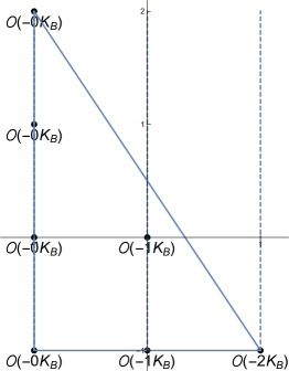
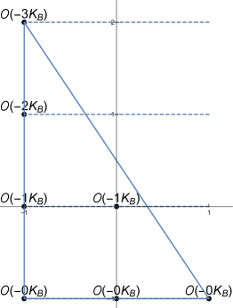
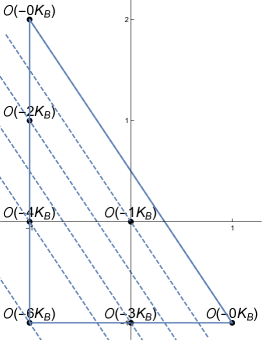
(a)	(b)	(c)

Figure 1: Different choices of the point $v^{(F)}_{s}$ used to specify a stacking construction are associated with different “twists” of the $F$-fiber bundle over the base $B$. The different choices of $v^{(F)}_{s}$ for a given fiber type give rise to monomials in the dual polytope that are sections of different line bundles over the base, illustrated here for three different choices of $v^{(F)}_{s}$ as vertices of the fiber $F_{10}=\mathbb{P}^{2,3,1}$. In the stacking construction, each lattice point in $\Delta_{2}$ is associated with a line bundle $\mathcal{O}(-(v^{(F)}_{s}\cdot m^{(F)}_{j}+1)K_{B}),m^{(F)}_{j}\in\Delta_{2}$. The dashed lines are normal to the corresponding $v^{(F)}_{s}$. The lattice points in $\Delta_{2}$ on the same dashed line are associated with sections of the same line bundle over the base. (cf. the $F_{10}$ data in Table 1 and Table 8.)

Given that $((v^{(B)}_{i})_{1,2},(v^{(F)}_{s})_{1,2})\in\nabla$ for all $i$ in a fibration that has the “stacked” form (2), the reflexive condition $m\cdot v\geq-1,m\in\Delta,v\in\nabla$ implies that a lattice point $m=((m^{(2)})_{1,2},(m^{(F)}_{j})_{1,2})\in\Delta$ gives a section in $\mathcal{O}(-(v^{(F)}_{s}\cdot m^{(F)}_{j}+1)K_{B})$. (See Figure 1 for examples with the $F_{10}$ fiber type, using the three different vertices $v^{(F)}_{s}$ of $\nabla_{2}$ as the specified points for three different stackings, including the “standard stacking” in which the monomials over the different lattice points in $\Delta_{2}$ correspond to sections $a_{n}$ of different line bundles in the Tate-form Weierstrass model.) Note that the lattice points in $\Delta$ that project to the same lattice point in $\Delta_{2}$ always give sections that belong to the same line bundle, since the line bundle depends only on $m^{(F)}_{j}$.

This shows that the allowed monomials in any polytope dual to a stacked fibration construction over a base $B$ take values as sections of various line bundles ${\cal O}(-nK_{B})$. For each vertex $v^{(F)}_{s}$ of the 2D polytope $\nabla_{2}$, and for each fiber type $F$, the number of lattice points in $\Delta_{2}$ corresponding to the resulting line bundle $\mathcal{O}(-nK)$ is listed in the third column in Table 8. For points $v^{(F)}_{s}$ in $\nabla_{2}$ that are not vertices, the numbers of such points will interpolate between the vertex values; the largest values of $n$ are found from vertex stackings.

The line bundles in which the monomials take sections place constraints on the structure of the base. The order of vanishing of a section $\sigma_{n}\in\mathcal{O}(-nK_{B})$ over a generic point in a rational curve $C$ with self-intersection $m=C\cdot C\leq-3$ is

$$\text{ord}_{C}(\sigma_{n})=\left\lceil\frac{n(m+2)}{m}\right\rceil.$$ (5)

The orders of vanishing $\{\text{ord}_{C}(\sigma_{n})\rvert n=1,2,3,4,(5),6\}$ for each $m$, $-3\geq m\geq-13$, are listed in the second column in Table 1. Note that none of the 16 fiber types gives a section of $\mathcal{O}(-5K_{B})$ (see the third column in Table 8).

For a Weierstrass model, where the coefficients $f,g$ are sections of the line bundles ${\cal O}(-4K_{B})$ and ${\cal O}(-6K_{B})$, the Kodaira condition that a singularity have a Calabi-Yau resolution is that $f,g$ cannot vanish to orders 4 and 6. For the more general class of fibrations we are considering here, the necessary condition is that at least one section $\sigma_{n=1,2,3,4,(5),6}$ exists with $\text{ord}_{C}(\sigma_{n})<n$. This condition is necessary so that when the sections are combined to make a Weierstrass form, the resulting $f,g$ give either a section in $\mathcal{O}(-4K_{B})$ or a section in $\mathcal{O}(-6K_{B})$, respectively, whose order of vanishing does not exceed $4$ or $6$. Note that as the absolute value $|m|$ of the self-intersection of the curve $C$ increases, the minimal $n$ that satisfies $\text{ord}_{C}(\sigma_{n})<n$ is non-decreasing. The minimum value min($n$) so that this condition is satisfied is listed for each $m$ in Table 2. Therefore, given a fiber type $F$ with a specified point $v^{(F)}_{s}$, the allowed negative curves in the base that are allowed for a stacking construction using the point $v^{(F)}_{s}$ that gives a resolvable Calabi-Yau construction are such that the following two conditions are satisfied: the existence of a section $\sigma_{n=1,2,3,4,\text{ or }6}$ such that (1) $\sigma_{n}\in\mathcal{O}(-(v^{(F)}_{s}\cdot m^{(F)}_{j}+1)K_{B})$ and (2) ord${}_{C}(\sigma_{n})<n$. For each fiber type $\nabla_{2}$, we have considered the stacking constructions over each vertex. The most negative self-intersection curve that is allowed in the base for each fiber type is tabulated in the last non-empty entry in the corresponding column in Table 1, and a $v^{(F)}_{s}$ that gives rise to stacked fibrations in which the most negative curve is allowed, and the corresponding line bundles associated with lattice points in $\Delta_{2}$ are given in Appendix B. Note that since for any lattice point in $\Delta_{2}$, the largest value of $n$ such that for any choice of stacking point $v^{(F)}_{s}$ the corresponding points in $\Delta$ are sections of ${\cal O}(-nK_{B})$ arises from a vertex, it is sufficient to consider the maximum $n$ across the possible choices of vertices $v^{(F)}_{s}$.

This analysis shows that any polytope that has the stacked form with a given fiber type $F$ gives a genus one fibration over a base $B$ in which the self-intersection of the curves has a lower bound given by the last nonempty entry in the corresponding column of Table 1. For the fiber $F_{10}$, this bound is more general. It is not possible to find any elliptic fibration with a smooth Calabi-Yau resolution over a base that contains curves of self-intersection $C\cdot C<-12$. While we have not proven it for polytopes that do not have the stacking form described here, it seems plausible to conjecture that the bounds on curves in the base for each fiber type given in Table 1 will also hold for arbitrary fibrations (i.e. for general “twists” of the fibration that do not have the stacking type). We have not encountered any cases in our analysis that would violate this conjecture. And it is straightforward to see using the analysis done here already that these curve bounds will still hold when there is a coordinate system where each ray of the base has a pre-image living over some ray $v_{F}\in\nabla_{2}$, even when these rays are not all the same $v^{(F)}_{s}$ as in the stacking case, since the bound applying for each curve will match that of some choice of $v^{(F)}_{s}$. If the more general conjecture is correct, then, for example, it would follow in general that any reflexive polytope with a fiber $F_{4}$ can only have curves in the base of self-intersection $\geq-8$, those with a fiber $F_{1}$ can only have curves in the base of self-intersection $\geq-6$, etc. We leave, however, a general proof of this assertion to further work.

2.4 Explicit construction of reflexive polytopes from stackings

In [23], we showed that the standard stacking construction with the fiber $\mathbb{P}^{2,3,1}$, combined with a large class of Tate-form Weierstrass tunings, can be used to explicitly construct a large fraction of the reflexive polytopes in the Kreuzer-Skarke database at large Hodge numbers. The stacking construction with other fibers can be used similarly to construct other reflexive polytopes in the KS database.

Explicitly, given the negative curve bounds on the base determined above, we can construct a stacked $F$-fibered polytope over $B$ as follows, following a parallel procedure to that described in [23] for the $\mathbb{P}^{2,3,1}$-fibered standard stackings: Given a fiber $F$ with a specified ray $v^{(F)}_{s}$, and a smooth 2D toric base $B$ in which the self-intersections of all curves are not lower than the negative curve bound associated with $v^{(F)}_{s}$, we start with the minimal fibered polytope $\tilde{\nabla}\subset N$ (which may not be reflexive) that is the convex hull of the set in equation (2). If $\tilde{\nabla}$ is reflexive, then we are done; otherwise we adopt the “dual of the dual” procedure used in [23] to resolve $\tilde{\nabla}$: define $\Delta^{\circ}=\text{ convex hull}((\tilde{\nabla})^{*}\cap M)$. As long as the negative curve bound is satisfied (no $(4,6)$ curves), $\Delta^{\circ}$ is a reflexive polytope, and the resolved polytope in $N$ is $\nabla\equiv(\Delta^{\circ})^{*}$.

Explicit examples of $F$-fibered polytopes over Hirzebruch surfaces $\mathbb{F}_{m}$ are given in Table 8, for each fiber type $F$. The base $\mathbb{F}_{m}$ is in each case chosen such that $-m$ saturates the negative curve bound associated with the specific vertex $v^{(F)}_{s}$ for a given fiber type (see Appendix B for the possible choices of $v^{(F)}_{s}$ for each fiber type that allow the most negative self-intersection curves in the base). For example, the standard stacked $\mathbb{P}^{2,3,1}$-fibered polytopes considered in [23] have bases stacked over the vertex $(-3,-2)$ of the fiber $F_{10}$ in Appendix A, and there exist sections in $\mathcal{O}(-nK_{B})$ for $n=1,2,3,4,6$ (see Figure (c) in Table 1), so models in this class correspond naturally to the Tate-form Weierstrass models where $a_{n}=\sigma_{n}$, and the negative curve bound is $-12$. The model listed in Table 8 is the generic elliptically fibered CY over $\mathbb{F}_{12}$.

The construction just described above gives the minimal reflexive $F$-fibered polytope over $B$ that contains the set in equation (2). While the $F_{10}$ fiber type with $v^{(F)}_{s}=(-3,-2)$ gives the most generic elliptic Calabi-Yau over any given toric base $B$ through this construction, using the other fiber types or the other specified points of $F_{10}$ for stacked stacking polytopes give models with enhanced symmetries (these can include discrete, abelian, and non-abelian symmetries). Further tunings of the polytope analogous to Tate-tunings for the standard $\mathbb{P}^{2,3,1}$ polytope can reduce $\Delta$ and enlarge $\nabla$, giving a much larger class of reflexive polytopes for Calabi-Yau threefolds. The explicit construction of the polytopes corresponding to Tate tuned models via polytope tunings of the standard $F_{10}$-fibered polytope with $v^{(F)}_{s}=(-3,-2)$ were discussed in section 4.3.3 and Appendix A in [23]. We have not attempted systematic polytope tunings for the other fiber types, but in principle one can work out tuning tables analogous to the Tate table for the other fiber types.

3 Results at large Hodge numbers

We have systematically run the algorithm described in Section 2.2 to check for a manifest elliptic or genus one fibration realized through a reflexive 2D fiber for each polytope in the Kreuzer-Skarke database that gives a Calabi-Yau threefold $X$ with $h^{1,1}(X)$ or $h^{2,1}(X)$ greater or equal to 140. The number of polytopes that give rise to Calabi-Yau threefolds with $h^{1,1}\geq 140$ is $248305$. Since the set of reflexive polytopes is mirror symmetric (Hodge numbers $h^{1,1},h^{2,1}$ are exchanged in going from $\nabla\leftrightarrow\Delta$), this is also the number of polytopes with $h^{2,1}\geq 140$. (Note, however, that the mirror of an elliptic Calabi-Yau threefold is not necessarily elliptic.) There are $495515$ polytopes with at least one of the Hodge numbers at least 140, and from these numbers it follows that the number of polytopes with both Hodge numbers at least 140 is $1095$. While as described in Section 2.2, we have made the algorithm reasonably efficient for larger values of $h^{1,1}$, our implementation in this initial investigation was in Mathematica, so a complete analysis of the database using this code was impractical. We anticipate that in the future a complete analysis of the rest of the database can be carried out with a more efficient code, but our focus here is on identifying the largest values of $h^{1,1},h^{2,1}$ that are associated with polytopes that give Calabi-Yau threefolds with no manifest elliptic fiber. In §4 we analyze the distribution of fibrations at small $h^{1,1}$.

3.1 Calabi-Yau threefolds without manifest genus one fibers

Of the 495515 polytopes analyzed at large Hodge numbers, we found that only four lacked a 2D reflexive polytope fiber, and thus the other 495511 polytopes all lead to Calabi-Yau threefolds with a manifest genus one fiber. The Hodge numbers of the four Calabi-Yau threefolds without a manifest genus one fiber are

$$(h^{1,1},h^{2,1})=(1,149),\hskip 7.22743pt(1,145),\hskip 7.22743pt(7,143),\hskip 7.22743pt(140,62)\,.$$ (6)

(See Figure 2.) It is of course natural that any Calabi-Yau threefold with $h^{1,1}=1$ cannot be elliptically fibered; by the Shioda-Tate-Wazir formula [39], any elliptically fibered Calabi-Yau threefold must have at least $h^{1,1}=2$, with one contribution from the fiber and at least one more from $h^{1,1}$ of the base, which must satisfy $h^{1,1}(B)\geq 1$. We also expect that any genus one fibered CY3 will have at least a multi-section [6, 7], so $h^{1,1}\geq 2$ in these cases for similar reasons.

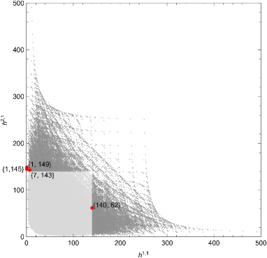
Figure 2: The four Hodge pairs in the region $h^{1,1}\geq 240$ or $h^{2,1}\geq 240$ associated with polytopes without reflexive 2D subpolytopes associated with genus one (including elliptic) fibers.

The examples (1, 145) and (1, 149) are the only Hodge numbers from polytopes in the Kreuzer-Skarke database with $h^{1,1}=1,h^{2,1}\geq 140$. Note that the quintic, with Hodge numbers (1, 101), is another example of a Calabi-Yau threefold with $h^{1,1}=1$ that has no elliptic or genus one fibration.

We list here the polytope structure of the two examples from (6) that have $h^{1,1}>1$, in the form given in the Kreuzer-Skarke database. M refers to the numbers of lattice points and vertices of the dual polytope $\Delta$, while N refers to the numbers of lattice points and vertices of the polytope $\nabla$, and H refers to the Hodge numbers $h^{1,1}$ and $h^{2,1}$. The vectors listed are the vertices of the polytope in the $N$ lattice. The numbers in parentheses for each polytope refer to the position in the list of polytopes in the Kreuzer-Skarke database that give CY3s with those specific Hodge numbers.

• M:196 5 N:10 5 H:7,143 (1${}^{\text{st}}$/54)

  Vertices of $\nabla$: $\{(-1,4,-1,-2),(-1,-1,1,1),(1,-1,0,0),(-1,-1,0,1),(-1,-1,0,3)\}$

• M:88 8 N:193 9 H:140,62 (6${}^{\text{th}}$/255)

  Vertices of $\nabla$: {$(-1,2,-1,4),(-1,0,4,-1),(1,-1,-1,-1),(-1,-1,-1,19),$

  $(-1,-1,5,1),(-1,1,0,-1),(-1,1,-1,-1),(-1,-1,-1,-1),(-1,-1,5,-1)$}

Note that we have not proven that these Calabi-Yau threefolds do not have elliptic or genus one fibers, we have just found that such fibers do not appear in a manifest form from the structure of the polytope. We leave for further work the question of analyzing non-toric elliptic or genus one fibration structure of these examples, or others with smaller Hodge numbers that also lack a manifest genus one fiber; such an analysis might be carried out using methods similar to those of [29].

3.2 Calabi-Yau threefolds without manifest elliptic fibers

Of the 495515 polytopes analyzed, only 384 had fibers of only types $F_{1},F_{2},F_{4}$. These cases are associated with genus one fibered Calabi-Yau threefolds that have no manifest toric section, and therefore are not necessarily elliptically fibered. Note that we have not proven that these Calabi-Yau threefolds do not have elliptic fibers; in fact, many toric hypersurface Calabi-Yau threefolds have been found to have non-toric fibrations [35]. It would be interesting to study these examples further for the presence of non-toric sections.

The largest values of $h^{2,1}$ and $h^{1,1}$ for these genus one fibered Calabi-Yau threefolds without a manifest toric section are realized by the examples:

• M:311 5 N:15 5 H:11, 227 (1${}^{\text{st}}$/19)

  Vertices of $\nabla$: $\{(-1,0,4,-3),(-1,2,-1,0),(1,-1,-1,1),(-1,0,-1,1),(-1,0,-1,3)\}$

• M:(80; 81; 81; 82) 8 N:(263; 262; 261; 260) 9 H:194, 56 ((7${}^{\text{th}}$; 8${}^{\text{th}}$; 9${}^{\text{th}}$; 10${}^{\text{th}}$)/52)

  Vertices of $\nabla$:

  • 7${}^{\text{th}}$ $\{(-1,0,4,-1),(-1,2,-1,-1),(1,-1,-1,-1),(-1,-1,-1,-1),(-1,-1,6,-1),\\ (-1,1,0,6),(-1,-1,-1,28),(-1,1,-1,10),(-1,-1,6,0)\}$,
    

  • 8${}^{\text{th}}$ $\{(-1,0,4,-1),(-1,2,-1,-1),(1,-1,-1,-1),(-1,-1,-1,-1),(-1,-1,6,-1),\\ (-1,1,0,6),(-1,-1,-1,28),(-1,0,-1,19),(-1,-1,6,0)\}$,
    

  • 9${}^{\text{th}}$ $\{(-1,0,4,-1),(-1,2,-1,-1),(1,-1,-1,-1),(-1,-1,-1,-1),(-1,-1,5,-1),\\ (-1,1,0,6),(-1,-1,-1,28),(-1,1,-1,10),(-1,-1,5,4)\}$,
    

  • 10${}^{\text{th}}$ $\{(-1,0,4,-1),(-1,2,-1,-1),(1,-1,-1,-1),(-1,-1,-1,-1),(-1,-1,5,-1),\\ (-1,1,0,6),(-1,-1,-1,28),(-1,0,-1,19),(-1,-1,5,4)\}$

The fiber type $F_{4}$ is the only fiber that arises in these five polytopes. In the first case, with Hodge numbers (11, 227), the base of the elliptic fibration is the Hirzebruch surface $\mathbb{F}_{8}$. Analysis of the F-theory physics of the genus one fibration associated with this polytope suggests that there should in fact be an elliptic fiber with a non-toric global section. For further work, it would be nice to prove this and find the non-toric section explicitly. Further analysis of the F-theory physics of the other cases may also be interesting, as well as the question of whether these threefolds admit elliptic fibrations that are not manifest in the toric description.

3.3 Fiber types

The numbers of distinct polytopes in the regions $h^{1,1},h^{2,1}\geq 140$ that have each fiber type (not counting multiplicities) are

$F_{1}$	$F_{2}$	$F_{3}$	$F_{4}$	$F_{5}$	$F_{6}$	$F_{7}$	$F_{8}$
612	1	1279	40218	32	19907	20	8579
$F_{9}$	$F_{10}$	$F_{11}$	$F_{12}$	$F_{13}$	$F_{14}$	$F_{15}$	$F_{16}$
2067	487387	24811	850	27631	2438	273	58

In Appendix C, we have included a set of figures that show the distribution of polytopes containing each fiber type, according to the Hodge numbers of the associated Calabi-Yau threefolds. We have shaded the data points of Hodge pairs varying from light to dark with increasing multiplicities; two factors contribute to the multiplicity in these figures: the multiplicity of the polytopes associated with the same Hodge pair and the multiplicity of fibers of the same type for a given polytope (note that the latter multiplicity is not included in the numbers in the table above). We discuss multiple fibrations in the next subsection.

We can see some interesting patterns in the distribution of polytopes with different fiber types. As discussed in §2.3, at least for polytopes with the stacked fibration form, the only fiber type that can arise over a base with a curve of self-intersection less than $-8$ is the $\mathbb{P}^{2,3,1}$ ($F_{10}$) fiber (see Table 1). From the graphs in Appendix C, it is clear that this fiber dominates at large Hodge numbers. The other fiber types that can arise over a base with a curve of self-intersection less than $-6$ are $F_{4},F_{13}$ (with two possible specified vertices) and $F_{6},F_{8},F_{11}$ (with only one specified vertex). The Hodge numbers of Calabi-Yau threefolds coming from polytopes with fiber types $F_{4},F_{6},F_{8}$ extend to $h^{1,1}=263$, and $F_{11}$ extends to $h^{1,1}=377$; in fact, the right most data point of the fiber types $F_{4},F_{6},F_{8},F_{9},F_{12},F_{15}$ is the same: $\{263,23\}$, and the right most data point of the fiber types $F_{11}$ and $F_{14}$ is the same: $\{377,11\}$. The fiber $F_{13}$ also continues out to the largest values of $h^{1,1}$ as $F_{10}$ does. Since the largest value of $h^{1,1}$ for a generic elliptic fibration over a toric base $B$ containing no curves of self-intersection $<-8$ is 224 [18, 19, 23], these large values of $h^{1,1}$ for fibers other than $F_{10}$ must involve tuning of relatively large gauge groups.

For $h^{1,1}>377$ the only fibers that arise are $F_{10}$ and $F_{13}$. In fact, the Calabi-Yau threefold with the largest $h^{1,1}$, which has Hodge numbers (491, 11), has two distinct fibrations: one has the standard $\mathbb{P}^{2,3,1}$ fiber over the 2D toric base {$-12//-11//-12//-12//-12//-12//-12//-12//-12//-12//-12//-12//-12//-12//-12//-11//-12,0$}, represented by the self-intersection numbers of the toric curves, where // stands for the sequence $-1,-2,-2,-3,-1,-5,-1,-3,-2,-2,-1$; the other fibration has the fiber $F_{13}$ over the base {$-4,-1,-3,-1,-4,-1,-4,-1,-4,0,2$}. We leave a more detailed analysis of the alternative fibration of this Calabi-Yau threefold for future work.

On the other hand, the fiber $F_{2}$, which is most restricted, arises from only one $\nabla$ polytope, with multiplicity one: M:40 6 N:186 6 H:149,29, which also has two different $F_{10}$ subpolytopes.

These observations tell us that, as we might expect, $h^{1,1}$ extends further for the fiber subpolytopes that admit more negative curves in the base. Almost half of the fiber types do not arise for any polytopes at all in the region $h^{2,1}\geq 140$: $F_{2},F_{5},F_{7},F_{12},F_{14},F_{15},$ and $F_{16}$. None of these is allowed over any base with a curve of self-intersection less than $-6$ (at least in the stacking construction of §2.3).

3.4 Multiple fibrations

Another interesting question is the prevalence of multiple fibrations. This question was investigated for complete intersection Calabi-Yau threefolds in [28, 29], where it was shown that many CICY threefolds have a large number of fibrations. In the toric hypersurface context we consider here, a polytope can have both multiple fibrations by different fiber types and by the same fiber type. In this analysis, as in the rest of this paper, we consider only fibrations that are manifest in the toric description. We have found that the total number of (manifest) fibrations in a polytope in the two large Hodge number regions ranges from zero to $58$. The total numbers of fibrations and the number of polytopes that have each number of total fibrations are listed in Table 3.

# fibrations	0	1	2	3	4	5	6
# polytopes	4	327058	113829	34657	11414	4466	1955
	(4)	(327058)	(113829)	(34659)	(11418)	(4465)	(1952)
# fibrations	7	8	9	10	11	12	13
# polytopes	1003	501	251	150	70	42	32
	(1003)	(503)	(251)	(149)	(71)	(42)	(32)
# fibrations	14	15	16	17	18	20	22
# polytopes	31	4	14	6	9	2	6
	(31)	(4)	(14)	(6)	(8)	(2)	(6)
# fibrations	23	25	26	31	34	37	58
# polytopes	2	1	2	1	1	3	1
	(1)	(1)	(2)	(1)	(1)	(2)	(0)

Table 3: Table of the number of polytopes in the large Hodge number regions $h^{1,1},h^{2,1}\geq 140$ that have a given number of distinct (manifest) fibrations. Numbers in parentheses are after modding out by automorphism symmetries (see text, Appendix D).

In some cases the number of fibrations is enhanced by the existence of automorphism symmetries of the polytope. While a generic polytope has no symmetries, some polytopes with large numbers of fibrations also have many symmetries. In such cases the number of inequivalent fibrations can be smaller than the total number of fibrations. This issue is also addressed in [34, 29]. There are 16 polytopes in the region $h^{1,1}\geq 140$ or $h^{2,1}\geq 140$ with a non-trivial action of the automorphism symmetry on the fibers. We list these 16 polytopes in Appendix D.1. For example, the polytope giving a Calabi-Yau with Hodge numbers (149, 1) has an automorphism symmetry of order 24, associated with an arbitrary permutation on 4 of the 5 vertices of the polytope. This automorphism symmetry group is described in detail in Appendix D.2; the number of distinct classes of fibrations modulo automorphisms in this case is reduced to only $8$ instead of 58.

The polytopes that we have found with a large total number of (manifest) fibrations are generally in the large $h^{1,1}$ region; in fact, polytopes in the large $h^{2,1}$ region have at most three fibrations:

# total fibrations	0	1	2	3
# polytopes with large $h^{2,1}$	3	240501	7775	26

The four polytopes with the two largest numbers of total fibrations (58, 37 without modding out by automorphisms) are respectively

$$\{\{7,5,201,5,149,1,296\},\{0,0,12,12,0,0,0,0,0,12,0,0,15,0,3,4\}\}$$

and

$$\{\{7,5,196,5,145,1,288\},\{0,0,0,6,0,6,0,0,0,12,0,0,9,3,0,1\}\}$$

$$\{\{8,6,195,7,144,2,284\},\{0,0,0,6,0,6,0,0,0,12,0,0,9,3,0,1\}\},$$

$$\{\{9,7,192,10,144,4,280\},\{0,0,0,0,0,9,0,0,0,15,3,0,6,3,0,1\}\},$$

where the numbers are in the format

{{# lattice points of $\Delta$, # vertices of $\Delta$, # lattice points of $\nabla$, # vertices of $\nabla$,

$h^{1,1}$, $h^{2,1}$, Euler Number},{#$F_{1}$,#$F_{2}$,$\ldots$,#$F_{16}$}}.

Note that the first two polytopes are, respectively, the mirrors of the first two polytopes (with $h^{1,1}=1$) without any fibrations in equation (6).

We also note that in general, the polytopes with larger numbers of total manifest fibrations fall within a specific range of values of $h^{1,1}$ and $h^{2,1}$ (at least in the ranges we have studied here). The ranges of $h^{1,1}$ and $h^{2,1}$ of the polytopes that have 8 or more fibrations (without considering automorphisms) are listed in Table 4. It may be interesting to note that in a somewhat different context, it was found in [40] that a large multiplicity of elliptically fibered fourfolds arises at a similar locus in the space of Hodge numbers, at intermediate values of $h^{1,1}$ and small values of $h^{3,1}$ (which counts the number of complex structure moduli, as does $h^{2,1}$ for Calabi-Yau threefolds). It would be interesting to understand whether these observations stem from a common origin.

# total fibrations $\geq$	8	9	10	11	12
$h^{1,1}$ range	[140,272]	[140,243]	[140,243]	[140,214]	[140,208]
$h^{2,1}$ range	[1, 19]	[1, 19]	[1, 16]	[1, 16]	[1, 12]
	13	14	15	16	17
	[140, 208]	[140, 208]	[140, 208]	[140, 208]	[141, 173]
	[1, 11]	[1, 9]	[1, 8]	[1, 8]	[1, 7]
	18	20	22	23	25
	[141, 173]	[141, 173]	[141, 173]	[141, 165]	[141, 154]
	[1, 7]	[1, 6]	[1, 6]	[1, 5]	[1, 5]
	26	31	34	37	58
	[141, 149]	[141, 149]	[141, 149]	[144, 149]	[149, 149]
	[1, 5]	[1, 5]	[1, 4]	[1, 4]	[1, 1]

Table 4: Ranges of Hodge numbers in which the polytopes with the largest numbers of fibrations (not including automorphisms) are localized.

It is also interesting to note that while every Calabi-Yau threefold with $h^{1,1}>335$ or $h^{2,1}>256$ has more than one fibration, the polytopes associated with the largest values of $h^{1,1}$ have precisely two manifest fibrations, and the average number of fibrations at large $h^{1,1}$ is close to 2. In Figure 3, we show the average number of fibrations for the polytopes associated with Calabi-Yau threefolds of Hodge numbers $h^{1,1}\geq 140$.

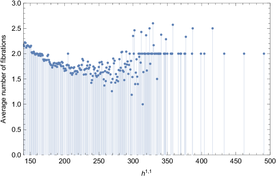
Figure 3: Average number of fibrations for polytopes associated with Calabi-Yau threefolds with $h^{1,1}\geq 140$.

The maximal number of fibrations for each specific fiber type in a polytope is

$F_{1}$	$F_{2}$	$F_{3}$	$F_{4}$	$F_{5}$	$F_{6}$	$F_{7}$	$F_{8}$	$F_{9}$	$F_{10}$	$F_{11}$	$F_{12}$	$F_{13}$	$F_{14}$	$F_{15}$	$F_{16}$
4	1	12	12	2	9	1	4	4	15	4	2	15	6	3	4
(4)	(1)	(6)	(8)	(2)	(9)	(1)	(4)	(4)	(15)	(4)	(2)	(9)	(6)	(3)	(1)

Numbers in parentheses are after modding out by automorphism symmetries; for example, the maximal number of $F_{16}$ fibers, which comes from the polytope associated with the Hodge pair (149,1), reduces from four to one (see the last row of the table in Appendix D.1).

If we count the distinct fiber types in a polytope, we find that the maximum number of fiber types that a polytope in the large Hodge number regions can have is eight. The eight polytopes that have the maximum number of eight distinct fiber types are

$$\{\{11,6,199,6,151,7,288\},\{0,0,2,1,0,0,0,2,0,3,2,0,2,1,1,0\}\},$$

$$\{\{12,7,193,8,146,8,276\},\{0,0,2,1,0,0,0,2,0,3,2,0,2,1,1,0\}\},$$

$$\{\{12,8,201,11,153,6,294\},\{0,0,2,0,0,2,0,0,0,3,2,2,1,1,0,1\}\},$$

$$\{\{13,8,198,10,151,7,288\},\{0,0,1,1,0,0,0,1,0,2,2,1,1,1,0,0\}\},$$

$$\{\{15,8,192,12,143,11,264\},\{0,0,2,2,0,1,0,2,0,3,1,0,1,0,1,0\}\},$$

$$\{\{14,9,184,12,140,8,264\},\{0,0,0,1,0,1,0,1,1,2,1,2,1,0,0,0\}\},$$

$$\{\{14,9,192,12,146,8,276\},\{0,0,1,1,0,0,0,1,0,2,2,1,1,1,0,0\}\},$$

$$\{\{16,9,191,13,143,11,264\},\{0,0,1,1,0,1,0,1,0,2,1,1,1,0,0,0\}\}.$$

In Table 5, we show the distribution of all polytopes, polytopes with large $h^{1,1}$, and polytopes with large $h^{2,1}$ according to the number of distinct fiber types. There are at most three distinct fiber types in the polytopes in $h^{2,1}\geq 140$. While all fiber types occur in the large $h^{1,1}$ region, the only fiber types that occur in the large $h^{2,1}$ region are $F_{1},F_{3},F_{4},F_{6},F_{8},F_{10},F_{11},$ and $F_{13}.$

# distinct fiber types	# polytopes	# polytopes with $h^{1,1}\geq 140$	# polytopes with $h^{2,1}\geq 140$
0	4	1	3
1	393788	153601	229443
2	86008	78995	6460
3	13354	13347	7
4	1755	1755	-
5	469	469	-
6	112	112	-
7	17	17	-
8	8	8	-

Table 5: Distribution of polytopes by number of distinct fiber types

Finally, it is interesting to note that only the plot of $F_{10}$ in Appendix C seems to exhibit mirror symmetry to any noticeable extent. We do not expect elliptic fibrations to respect mirror symmetry, so this may simply arise from a combination of the observation that the total set of hypersurface Calabi-Yau Hodge numbers in the Kreuzer-Skarke database is mirror symmetric and the observation that in the large Hodge number regions that we have considered most of the Calabi-Yau threefolds admit elliptic fibrations described by a $F_{10}$ fibration of the associated polytope.

3.5 Standard vs. non-standard $\mathbb{P}^{2,3,1}$-fibered polytopes

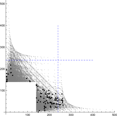
Figure 4: Hodge pairs with only non-standard $F_{10}$-fibered polytopes. The grey dots correspond to all Hodge pairs with $F_{10}$ fibers. The black dots correspond to Hodge pairs with only non-standard $F_{10}$-fibered polytopes. The vertical and horizontal dashed line correspond to $h^{1,1}=240$ and $h^{2,1}=240$, respectively.

In [23], we compared elliptic and toric hypersurface Calabi-Yau threefolds with Hodge numbers $h^{1,1}\geq 240$ or $h^{2,1}\geq 240$. We found that in the large $h^{1,1}$ region, there were eight Hodge pairs in the KS database that were not realized by a simple Tate-tuned model, and do not correspond to a “standard stacking” $\mathbb{P}^{2,3,1}$-fibered polytope. We found, however, that these eight outlying polytopes have a description in terms of a $\mathbb{P}^{2,3,1}$ fiber structure that is not of the standard ($v^{(F)}_{s}=(-3,-2)$) stacking form, and furthermore it can be seen do not respect the stacking framework of §2.3. The Weierstrass models of these Calabi-Yau threefolds all have the novel feature that they can have gauge groups tuned over non-toric curves, which can be of higher genus, in the base. As discussed in [23], the definition of a standard $\mathbb{P}^{2,3,1}$-fibered polytope $\nabla$ (where the base is stacked over the vertex $(-3,-2)$ of the $F_{10}$ fiber) turns out to be equivalent to the condition that the corresponding $\Delta$ has a single lattice point for each of the choices $m^{(F)}_{2}=(1,-1)$ and $m^{(F)}_{3}=(-1,2)$ in equation (3) (where we have numbered the vertex with the largest multiple of $-K_{B}$ as $m^{(F)}_{1}=(-1,-1)$), and there is furthermore a coordinate system in which this lattice point has coordinates $m^{(2)}=(0,0)$ in both cases. We have scanned through the $F_{10}$-fibered polytopes and used this feature to compute the fraction of $F_{10}$-fibered polytopes that have the standard versus non-standard form; the results of this analysis are shown in Table 6.

	total # fibrations	# fibrations in polytopes with $h^{1,1}\geq 140$	# fibrations in polytopes with $h^{2,1}\geq 140$
standard	433827	242562	192218
non-standard	183818	130255	53705
non-standard fraction	0.297611	0.349381	0.218381

Table 6: Fractions of fibrations by the fiber $F_{10}$ that take the “standard stacking” form versus other fibrations.

Of the 488119 $F_{10}$-fibered polytopes, 98758 have more than one $F_{10}$ fiber. Most of these polytopes have both standard and non-standard types of fibrations. There are 103 Hodge pairs that have only the non-standard fibered polytopes. These may give rise to more interesting Weierstrass models, like those we have studied with $h^{1,1}\geq 240$ in section 6.2 of [23]. As a crosscheck to the “sieving” results there, we have confirmed that none of these 103 Hodge pairs are in the region $h^{2,1}\geq 240$, and the 12 Hodge pairs of these 103 pairs that have $h^{1,1}\geq 240$ are exactly the Hodge pairs associated with non-standard $\mathbb{P}^{2,3,1}$-fibered polytopes in Table 17 of [23], together with the four Hodge pairs of Bl${}_{[0,0,1]}\mathbb{P}^{2,3,1}$-fibered polytopes; the latter four polytopes, in other words, happen to also be $F_{11}$-fibered, and can be analyzed as blowups of standard $\mathbb{P}^{2,3,1}$ model (U(1) models). We list the remaining 91 Hodge pairs that only have non-standard $\mathbb{P}^{2,3,1}$ fiber types below (see also Figure 4):

• $140\leq h^{1,1}<240$
  $\{\{149,1\},\{154,7\},\{179,8\},\{177,16\},\{179,22\},\{207,22\},\{235,22\},\{184,23\},\{228,24\}$,
  $\{178,27\},\{206,27\},\{177,28\},\{205,28\},\{211,38\},\{232,38\},\{233,38\},\{182,39\},\{217,39\}$,
  $\{223,40\},\{194,41\},\{221,41\},\{210,43\},\{203,44\},\{174,45\},\{207,45\},\{145,46\},\{193,46\}$,
  $\{205,46\},\{159,48\},\{180,49\},\{187,53\},\{239,53\},\{150,55\},\{231,55\},\{225,57\},\{231,57\},$
  $\{204,63\},\{231,63\},\{175,64\},\{237,65\},\{141,66\},\{208,66\},\{228,66\},\{199,67\},\{211,67\},$
  $\{193,69\},\{201,69\},\{190,70\},\{200,70\},\{161,71\},\{160,73\},\{190,76\},\{214,82\},\{185,83\},$
  $\{198,84\},\{181,85\},\{193,85\},\{229,85\},\{164,86\},\{200,86\},\{160,88\},\{185,93\},\{177,101\}$,
  $\{197,101\},\{148,102\},\{171,105\},\{147,119\},\{141,123\},\{140,126\}\}$

• $140\leq h^{2,1}<240$
  $\{\{3,141\},\{3,165\},\{3,195\},\{4,142\},\{4,148\},\{4,154\},\{4,162\},\{4,166\},\{4,178\},\{5,141\}$,
  $\{5,143\},\{5,149\},\{5,153\},\{11,176\},\{22,217\},\{23,182\},\{23,200\},\{24,183\},\{31,170\}$,
  $\{95,155\},\{110,144\},\{111,141\}\}$.

4 Fibration prevalence as a function of $h^{1,1}(X)$

In this section we consider the fraction of Calabi-Yau threefolds at a given value of the Picard number $h^{1,1}(X)$ that admit a genus one or elliptic fibration. We begin in §4.1 with a summary of some analytic arguments for why we expect that an increasingly small fraction of Calabi-Yau threefolds will fail to have such a fibration as $h^{1,1}$ increases; we then present some preliminary numerical results in §4.2.

4.1 Cubic intersection forms and genus one fibrations

For some years, mathematicians have speculated that the structure of the triple intersection form on a Calabi-Yau threefold may make the existence of a genus one or elliptic fibration increasingly likely as the Picard number $\rho(X)=h^{1,1}(X)$ increases. The rationale for this argument basically boils down to the fact that a cubic in $k$ variables is increasingly likely to have a rational solution as $k$ increases. In this section we give some simple arguments that explain why in the absence of unexpected conspiracies this conclusion is true. If this result could be made rigorous it would be a significant step forwards towards proving the finiteness of the number of distinct topological types of Calabi-Yau threefolds.

As summarized in [28], the following conjecture is due to Kollár [41]:

Conjecture 1.

Given a Calabi-Yau $n$-fold $X$, $X$ is genus one (or elliptically) fibered iff there exists a divisor $D\in H^{2}(X,\mathbb{Q})$ that satisfies $D^{n}=0,D^{n-1}\neq 0$, and $D\cdot C\geq 0$ for all algebraic curves $C\subset X$.

Basically the idea is that $D$ corresponds to the lift $D=\pi^{-1}(D^{(B)})$ of a divisor $D^{(B)}$ on the base of the fibration, where the $(n-1)$-fold self-intersection of $D$ gives a positive multiple of the fiber $F=\pi^{-1}(p)$, with $p$ a point on the base. This conjecture was proven already for $n=3$ by Oguiso and Wilson [42, 43] under the additional assumption that either $D$ is effective or $D\cdot c_{2}(X)\neq 0$. In the remainder of this section, as elsewhere in the paper, we often simply refer to a Calabi-Yau as genus one fibered as a condition that includes both elliptically fibered Calabi-Yau threefolds and more general genus one fibered threefolds.

In the case $n=3$, to show that a Calabi-Yau threefold is genus one fibered, we thus wish to identify an effective divisor $D$ whose triple intersection with itself vanishes. The triple intersection form can be written in a particular basis $D_{i}$ for $H^{2}(X,\mathbb{Z})$ as

$$\langle A,B,C\rangle=\sum_{i,j,k}\kappa_{ijk}a_{i}b_{j}c_{k}\,,$$ (7)

where $A=\sum_{i}a_{i}D_{i}$, etc., and $D_{i}\cap D_{j}\cap D_{k}=\kappa_{ijk}$ The condition that there is a divisor $D=\sum_{i}d_{i}D_{i}$ satisfying $D^{3}=0$ is then the condition that the cubic intersection form on $D$ vanishes

$$D^{3}=\langle D,D,D\rangle=\sum_{i,j,k}\kappa_{ijk}d_{i}d_{j}d_{k}=0\,.$$ (8)

We are thus interested in finding a solution over the rational numbers of a cubic equation in $k=\rho(X)$ variables. The curve condition provides a further constraint that $D$ lies in the positive cone defined by $D\cdot C\geq 0$ for all algebraic curves $C\subset X$. Note that identifying a rational solution $D$ to (8) immediately leads to a solution over the integers $\hat{d}_{i}\in\mathbb{Z}\ \forall i$, simply by multiplying by the LCM of all the denominators of the rational solution $d_{i}$.

There are basically two distinct ways in which the conditions for the existence of a divisor in the positive cone satisfying $D^{3}=0$ can fail. We consider each in turn. Note that even when the condition $D^{3}=0$ is satisfied, the condition for an elliptic fibration can fail if $D^{2}=0$, in which case $D$ itself corresponds to a K3 fiber; this class of fibrations is also interesting to consider but seems statistically likely to become rarer as $\rho$ increases.

4.1.1 Number theoretic obstructions

There can be a number theoretic obstruction to the existence of a solution to a degree $n$ homogeneous equation over the rationals such as (8). For example, there cannot be an integer solution in the variables $x,y,z,w$ of the equation

$$x^{3}+x^{2}y+y^{3}+2z^{3}+4w^{3}=0\,.$$ (9)

This can be seen as follows: if all the variables $x,y,z,w$ are even, we divide by the largest possible power of 2 that leaves them all as integers. Then there must be a solution with at least one variable odd. The variable $x$ cannot be odd, since if $y$ is odd or even the LHS is odd. Similarly, $y$ cannot be odd. So $x,y$ must be even in the minimal solution. But $z$ cannot be odd or the LHS would be congruent to 2 mod 4. And $w$ cannot be odd if the others are even since then the LHS would be congruent to 4 mod 8.

Such number-theoretic obstructions can only arise for small numbers of variables $k$. It was conjectured long ago that for a homogeneous degree $n$ polynomial the maximum number of variables for which such a number-theoretic obstruction can arise is $n^{2}$ [44]. While there is a counterexample known for $n=4$, where there is an obstruction for a quartic with 17 variables, it was proven in [45] that every non-singular cubic form in 10 variables with rational coefficients has a non-trivial rational zero. And the existence of a rational solution has been proven for general (singular or non-singular) cubics in 16 or more variables [46]. Thus, no number-theoretic obstruction to the existence of a solution to $D^{3}=0$ can arise when $\rho(X)=h^{1,1}(X)>15$, and there are also quite likely no obstructions for $\rho(X)>9$ though this stronger bound is not proven as far as the authors are aware.

4.1.2 Cone obstructions

If the coefficients in the cubic conspire in an appropriate way, the cubic can fail to have any solutions in the Kähler cone. We now consider this type of obstruction to the existence of a solution. For example, the cubic

$$\sum_{i}d_{i}^{3}+\sum_{i,j}d_{i}^{2}d_{j}+\sum_{i,j,k}d_{i}d_{j}d_{k}=0$$ (10)

has no nontrivial solutions in the cone $d_{i}\geq 0$ since all coefficients are positive. The absence of solutions in a given cone becomes increasingly unlikely, however, as the number of variables increases (again, in the absence of highly structured cubic coefficients). A somewhat rough and naive approach to understanding this is to consider adding the variables one at a time, assuming that the coefficients are random and independently distributed numbers. In this analysis we do not worry about the existence of rational solutions; in any given region, the existence of a rational solution should depend upon the kind of argument described in the previous subsection. We assume for simplicity that the cone condition states simply that $d_{i}\geq 0\ \forall i$; a more careful analysis would consider cones of different sizes and angles. For two variables $x=d_{1},y=d_{2}$ we have a cubic equation

$$\kappa_{111}x^{3}+3\kappa_{112}x^{2}y+3\kappa_{122}xy^{2}+\kappa_{222}y^{3}\,.$$ (11)

Now assume that $x$ is some fixed value $x\geq 0$. This cubic always has at least one real solution $(x,y)$. If the coefficients in the cubic are randomly distributed, we expect roughly a 1/2 chance that $y\geq 0$ for this real solution. Now add a third variable. If the above procedure gives a solution $(x,y,z=d_{3}=0)$ in the positive cone, we are done. If not, we plug in some fixed positive values $x,y\geq 0$ and the condition becomes a cubic in $z$. Again, there is statistically roughly a 1/2 chance that a given real solution for $z$ is positive. So for 3 variables we expect at most a probability of roughly $1/4$ that there is no solution in the desired cone. Similarly, for $k$ variables, this simple argument suggests that most a fraction of $1/2^{k-1}$ of random cubics will lack a solution in the desired cone.

This is an extremely rough argument, and should not be taken particularly seriously, but hopefully it illustrates the general sense of how it becomes increasingly difficult to construct a cubic that has no solutions in $k$ variables within a desired cone. Interestingly, the rate of decrease found by this simple analysis matches quite closely with what we find in a numerical analysis of the Kreuzer-Skarke data at small $k=\rho(X)=h^{1,1}(X)$.

4.2 Numerical results for Calabi-Yau threefolds at small $h^{1,1}(X)$

We have done some preliminary analysis of the distribution of polytopes without a manifest reflexive 2D fiber for cases giving Calabi-Yau threefolds with small $h^{1,1}$. The results of this are shown in Table 7.

It is interesting to note that the fraction of polytopes without a genus one (or elliptic) fiber that is manifest in the toric geometry decreases roughly exponentially, approximately as $p({\rm no\,fiber})\sim 0.1\times 2^{5-h^{1,1}}$ in the range $h^{1,1}\sim 4$—$7$. Comparing to the total numbers of polytopes in the KS database that lack a manifested genus one fiber, if this fraction continues to exhibit this pattern, the total number of polytopes out of the 400 million in the full KS database would be something like 14,000. (Note, however, that the polytope identified in the database that has no manifest fibration and corresponds to a Calabi-Yau with $h^{1,1}=140$ would be extremely unlikely if this exponential rate of decrease in manifest fibrations continues; this suggests that the tail of the distribution of polytopes lacking a manifest fibration does not decrease quite so quickly at large values of $h^{1,1}$. Because the analytic argument of the previous section involves all fibrations, not just manifest ones, it may be that this asymptotic is still a good estimate of actual fibrations if most of the polytopes at large $h^{1,1}$ that lack manifest fibrations actually have other fibrations that cannot be seen from toric fibers.)

The naive distribution of the estimated number of polytopes from the simple exponentially decreasing estimate is shown in the black dots in Figure 5. Even with some uncertainty about the exact structure of the tail of this distribution, this seems to give good circumstantial evidence that at least among this family of Calabi-Yau threefolds, the vast majority are genus one or elliptically fibered, and that the Calabi-Yau threefolds like the quintic that lack genus one fibration structure are exceptional rare cases, rather than the general rule.

$h^{1,1}$	$2$	$3$	$4$	$5$	$6$	$7$
Total # polytopes	$36$	$244$	$1197$	$4990$	$17101$	$50376$
# without reflexive fiber $\nabla_{2}$	$23$	$91$	$256$	$562$	$872$	$1202$
% without reflexive fiber	$0.639$	$0.373$	$0.214$	$0.113$	$0.051$	$0.024$

Table 7: The numbers of polytopes without a 2D reflexive fiber, corresponding to Calabi-Yau threefolds without a manifest genus one fibration, for small values of $h^{1,1}$

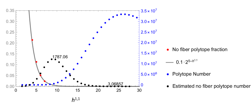
Figure 5: The fraction of polytopes without a manifest reflexive fiber goes roughly as $0.1\times 2^{5-h^{1,1}}$ for small values of $h^{1,1}$. Continuing this estimate to higher values of $h^{1,1}$, the estimated number of polytopes with no fiber has a peak value around $1800$ at $h^{1,1}\sim 9$ and drops below five around $h^{1,1}\sim 24$. The estimated number of total polytopes with no manifest fiber is around $14,000$.

5 Conclusions

The results reported in this paper indicate that most Calabi-Yau threefolds that are realized as hypersurfaces in toric varieties have the form of a genus one fibration. At large Hodge numbers almost all Calabi-Yau threefolds in the Kreuzer Skarke database satisfy the stronger condition that they are elliptically fibered. This contributes to the growing body of evidence that most Calabi-Yau threefolds lie in the finite class of elliptic fibrations. We have shown that all known Calabi-Yau threefolds where at least one of the Hodge numbers is greater than 150 must have a genus one fibration, and all CY3’s with $h^{1,1}\geq 195$ or $h^{2,1}\geq 228$ have an elliptic fibration. We have also shown that the fraction of toric hypersurface Calabi-Yau threefolds that are not manifestly genus one fibered decreases exponentially roughly as $0.1\times 2^{5-h^{1,1}}$ for small values of $h^{1,1}$. These results correspond well with the recent investigations in [28, 29, 47], which showed that over 99% of all complete intersection Calabi-Yau (CICY) threefolds have a genus one fibration (and generally many distinct fibrations), including all CICY threefolds with $h^{1,1}>4$, and that similar results hold for the only substantial known class of non-simply connected Calabi-Yau threefolds.

Taken together, these empirical results, along with the analytic arguments described in §4.1, suggest that it becomes increasingly difficult to form a Calabi-Yau geometry that is not genus one or elliptically fibered as the Hodge number $h^{1,1}$ increases. Proving that any Calabi-Yau with Hodge numbers beyond a certain value must admit an elliptic fibration is a significant challenge for mathematicians; progress in this direction might help begin to place some explicit bounds that would help in proving the finiteness of the complete set of Calabi-Yau threefolds.

There are a number of ways in which the analysis of this paper could be extended. Clearly, it would be desirable to analyze the fibration structure of the full set of polytopes in the Kreuzer-Skarke database, which could be done by implementing the algorithm used in this paper using faster and more powerful computational tools. It is also important to note that while the simple criteria we used here showed already that most known Calabi-Yau threefolds at large Hodge numbers are elliptic or more generally genus one fibered, the cases that are not recognized as fibered by these simple criteria may still have genus one or elliptic fibers. In particular, while we have identified a couple of Calabi-Yau threefolds with $h^{1,1}>1$ and either $h^{1,1}$ or $h^{2,1}$ greater than 140 that do not admit an explicit toric genus one fibration that can be identified by a 2D reflexive fiber in the 4D polytope, it seems quite likely that the Calabi-Yau threefolds associated with these polytopes may have a non-toric genus one or elliptic fibration structure. Such fibrations could be identified by a more extensive analysis along the lines of [29].

For Calabi-Yau threefolds that do not admit any genus one or elliptic fibration, it would be interesting to understand whether there is some underlying structure to the triple intersection numbers that is related to those of elliptically fibered Calabi-Yau manifolds, and whether there are simple general classes of transitions that connect the non-elliptically fibered threefolds to the elliptically fibered CY3’s, which themselves all form a connected set through transitions associated with blow-ups of the base and Higgsing/unHiggsing processes in the corresponding F-theory models. We leave further investigation of these questions for future work.

Finally, it of course would be interesting to extend this kind of analysis to Calabi-Yau fourfolds. An early analysis of the fibration structure of some known toric hypersurface Calabi-Yau fourfolds was carried out in [48]. The analysis of fibration structures of complete intersection Calabi-Yau fourfolds in [25] suggests that again most known constructions should lead predominantly to Calabi-Yau fourfolds that are genus one or elliptically fibered. The classification of hypersurfaces in reflexive 5D polytopes has not been completed, although the complete set of $3.2\times 10^{11}$ associated weight systems has recently been constructed [49]. In fact, recent work on classifying toric threefold bases that can support elliptic Calabi-Yau fourfolds suggests that the number of such distinct bases already reaches enormous cardinality on the order of $10^{3000}$ [50, 40]. Thus, at this point the known set of elliptic Calabi-Yau fourfolds is much larger than any known class of Calabi-Yau fourfolds from any other construction.

Appendix A The 16 reflexive 2D fiber polytopes $\nabla_{2}$

We list here the 16 reflexive 2D polytopes $\nabla_{2}$. The dual polytopes $\Delta_{2}$ are listed in Appendix B. With each polytope we also provide the value $I_{\rm max}$ associated with the maximum possible value of $v\cdot m$ where $v\in\nabla_{2},m\in\Delta_{2}$. As discussed in the main text, the three fibers $F_{1}=\mathbb{P}^{2},F_{2}=\mathbb{P}^{1}\times\mathbb{P}^{1}=\mathbb{F}_{0},F_{4}=\mathbb{F}_{2}$ have no $-1$ curves, associated with divisors that give global sections; all other fibers have $-1$ curves and correspond to elliptic fibers of the Calabi-Yau threefold.

Appendix B The 16 dual polytopes $\Delta_{2}$

The dual polytopes $\Delta_{2}$ for the 16 reflexive 2D fiber polytopes listed in the previous Appendix. For each fiber type $\nabla_{2}$ in Appendix A, a lattice point $v^{(F)}\in\nabla_{2}$ is given such that a fibration built from the stacking construction (§2.3.1) over the point $v^{(F)}$ allows the most negative curve self-intersection in the base among all stackings with that fiber.

Appendix C Distribution of polytopes with each fiber type

The figures in this Appendix depict the distribution of Hodge numbers for the Calabi-Yau threefolds associated with the polytopes that have each type of reflexive 2D fiber. The largest values of $h^{1,1}$ and $h^{2,1}$ for Calabi-Yau threefolds associated with polytopes having each fiber type are shown in the figure. In each figure, the density scale at the right indicates the color coding according to the total number of fibrations at each Hodge number pair, which results both from the multiplicity of the fibers of a given polytope and from the multiplicity of the polytopes at each Hodge number pair.

$F$	$v^{(F)}_{s}$	{#pts${}_{\Delta_{2}}(\mathcal{O}(-nK_{B}))\rvert$ $n=0,1,2,3,4,(5),6$}	fibered-polytope	$B$
$F_{1}$	$(1,0),(0,1),(-1,-1)$	$\{4,3,2,1,0,(0),0\}$	M:171 5 N:11 5 H:11,131	$\mathbb{F}_{6}$
$F_{2}$	$(1,0),(0,1),(0,-1),(-1,0)$	$\{3,3,3,0,0,(0),0\}$	M:117 8 N:11 6 H:9,93	$\mathbb{F}_{4}$
$F_{3}$	$(1,1)$	$\{2,3,4,0,0,(0),0\}$	M:144 8 N:11 6 H:8,110	$\mathbb{F}_{4}$
	$(1,0),(0,1)$	$\{3,3,2,1,0,(0),0\}$	M:170 9 N:14 7 H:11,131	$\mathbb{F}_{6}$
	$(-1,-1)$	$\{4,3,2,0,0,(0),0\}$	M:90 8 N:11 6 H:10,76	$\mathbb{F}_{4}$
$F_{4}$	$(1,0)$	$\{5,3,1,0,0,(0),0\}$	M:63 5 N:11 5 H:11,59	$\mathbb{F}_{4}$
	$(-1,1),(-1,-1)$	$\{3,2,2,1,1,(0),0\}$	M:311 5 N:15 5 H:11,227	$\mathbb{F}_{8}$
$F_{5}$	$(1,0),(0,1)$	$\{3,3,2,0,0,(0),0\}$	M:89 12 N:13 8 H:10,76	$\mathbb{F}_{4}$
	$(0,-1),(-1,0)$	$\{2,3,3,0,0,(0),0\}$	M:116 12 N:13 8 H:9,93	$\mathbb{F}_{4}$
	$(-1,-1)$	$\{2,3,2,1,0,(0),0\}$	M:169 13 N:17 9 H:11,131	$\mathbb{F}_{6}$
$F_{6}$	$(1,0)$	$\{4,3,1,0,0,(0),0\}$	M:62 9 N:13 7 H:11,59	$\mathbb{F}_{4}$
	$(0,1)$	$\{2,3,2,1,0,(0),0\}$	M:169 9 N:19 7 H:14,130	$\mathbb{F}_{6}$
	$(-1,1)$	$\{2,2,2,1,1,(0),0\}$	M:310 9 N:19 7 H:11,227	$\mathbb{F}_{8}$
	$(-1,-1)$	$\{3,2,2,1,0,(0),0\}$	M:158 9 N:16 7 H:11,131	$\mathbb{F}_{6}$
$F_{7}$	$(1,1),(1,0),(0,1),$ $(0,-1),(-1,0),(-1,-1)$	$\{2,3,2,0,0,(0),0\}$	M:88 16 N:15 10 H:10,76[3]	$\mathbb{F}_{4}$
$F_{8}$	$(1,1)$	$\{2,2,3,0,0,(0),0\}$	M:106 8 N:14 6 H:9,93	$\mathbb{F}_{8}$
	$(1,0)$	$\{3,3,1,0,0,(0),0\}$	M:61 9 N:16 7 H:12,58	$\mathbb{F}_{4}$
	$(-1,1)$	$\{2,1,2,1,1,(0),0\}$	M:296 9 N:22 7 H:11,227	$\mathbb{F}_{8}$
	$(-1,-1)$	$\{3,2,2,0,0,(0),0\}$	M:79 8 N:14 6 H:10,76	$\mathbb{F}_{4}$
$F_{9}$	$(1,0)$	$\{3,3,1,0,0,(0),0\}$	M:61 13 N:15 9 H:11,59	$\mathbb{F}_{4}$
	$(0,1),(0,-1)$	$\{2,3,2,0,0,(0),0\}$	M:88 12 N:16 8 H:11,75[2]	$\mathbb{F}_{4}$
	$(-1,1),(-1,-1)$	$\{2,2,2,1,0,(0),0\}$	M:144 14 N:19 10 H:12,120	$\mathbb{F}_{6}$
$F_{10}$	$(1,0)$	$\{4,2,1,0,0,(0),0\}$	M:63 5 N:11 5 H:11,59	$\mathbb{F}_{4}$
	$(0,1)$	$\{3,2,1,1,0,(0),0\}$	M:125 5 N:17 5 H:11,131	$\mathbb{F}_{6}$
	$(-3,-2)$	$\{2,1,1,1,1,(0),1\}$	M:680 5 N:26 5 H:11,491	$\mathbb{F}_{12}$
$F_{11}$	$(1,0)$	$\{3,2,1,0,0,(0),0\}$	M:51 9 N:16 7 H:11,59	$\mathbb{F}_{4}$
	$(-1,2)$	$\{2,1,1,1,1,(0),0\}$	M:257 9 N:24 7 H:11,227	$\mathbb{F}_{8}$
	$(0,-1)$	$\{2,3,1,0,0,(0),0\}$	M:60 9 N:20 7 H:15,57[2]	$\mathbb{F}_{4}$
	$(-1,-1)$	$\{2,2,1,1,0,(0),0\}$	M:124 9 N:20 7 H:11,131	$\mathbb{F}_{6}$
$F_{12}$	$(1,0),(0,1)$	$\{2,3,1,0,0,(0),0\}$	M:60 13 N:18 9 H:12,58	$\mathbb{F}_{4}$
	$(1,-1),(-1,1)$	$\{2,2,2,0,0,(0),0\}$	M:78 12 N:16 8 H:10,76	$\mathbb{F}_{4}$
	$(-1,-1)$	$\{2,1,2,1,0,(0),0\}$	M:145 13 N:21 9 H:11,131	$\mathbb{F}_{6}$
$F_{13}$	$(1,0)$	$\{3,1,1,0,0,(0),0\}$	M:60 13 N:18 9 H:12,58	$\mathbb{F}_{4}$
	$(-1,2),(-1,-2)$	$\{2,1,1,0,1,(0),0\}$	M:181 5 N:25 5 H:11,227	$\mathbb{F}_{8}$
$F_{14}$	$(2,-1),(-1,2)$	$\{2,1,1,1,0,(0),0\}$	M:112 9 N:22 7 H:11,131	$\mathbb{F}_{6}$
	$(0,-1),(-1,0)$	$\{2,2,1,0,0,(0),0\}$	M:50 9 N:19 7 H:12,58	$\mathbb{F}_{4}$
$F_{15}$	$(-1,1),(1,1),(-1,-1),(1,-1)$	$\{2,1,2,0,0,(0),0\}$	M:68 8 N:17 6 H:10,76	$\mathbb{F}_{4}$
$F_{16}$	$(2,-1),(-1,2),(-1,-1)$	$\{2,1,0,1,0,(0),0\}$	M:79 5 N:23 5 H:11,131	$\mathbb{F}_{6}$

Table 8: Line bundles in the $v_{s}$ stacking $F$-fibered construction, with examples over Hirzebruch surfaces $\mathbb{F}_{m}$, where $-m$ saturates the negative curve bound in each case.

Appendix D Automorphism symmetries and fibrations

D.1 Polytopes with non-trivial fibration orbits in the regions $h^{1,1},h^{2,1}\geq 140$

The following table indicates the difference between the total number of fibrations and the number of inequivalent fibration classes under automorphisms in the relevant 16 cases.

polytope data (in the format of the KS database)	# fibrations for each of the 16 fibers # fibrations modulo the automorphism symmetry group
M:12 5 N:348 5 H:251,5 [[492]]	0	0	0	0	0	0	0	0	0	3	0	0	1	0	0	0
	0	0	0	0	0	0	0	0	0	2	0	0	1	0	0	0
M:15 5 N:179 5 H:151,7 [[288]]	0	0	0	2	0	0	0	0	0	1	0	0	1	0	0	0
	0	0	0	1	0	0	0	0	0	1	0	0	1	0	0	0
M:14 5 N:196 5 H:161,5 [[312]]	0	0	0	2	0	0	0	0	0	2	0	0	1	0	0	0
	0	0	0	1	0	0	0	0	0	2	0	0	1	0	0	0
M:15 5 N:311 5 H:227,11 [[432]]	0	0	0	0	0	0	0	0	0	2	0	0	3	0	0	0
	0	0	0	0	0	0	0	0	0	1	0	0	3	0	0	0
M:17 5 N:177 5 H:151,7 [[288]]	0	0	0	2	0	0	0	0	0	3	0	0	0	0	0	0
	0	0	0	2	0	0	0	0	0	2	0	0	0	0	0	0
M:11 5 N:335 5 H:243,3 [[480]]	0	0	0	0	0	0	0	0	0	3	0	0	3	0	0	0
	0	0	0	0	0	0	0	0	0	2	0	0	3	0	0	0
M:13 5 N:117 5 H:148,4 [[288]]	0	0	0	1	0	0	0	0	0	2	0	0	3	0	0	0
	0	0	0	1	0	0	0	0	0	1	0	0	3	0	0	0
M:13 5 N:267 5 H:208,4 [[408]]	0	0	0	2	0	0	0	0	0	3	0	0	1	0	0	0
	0	0	0	1	0	0	0	0	0	2	0	0	1	0	0	0
M:10 5 N:376 5 H:272,2 [[540]]	0	0	0	0	0	0	0	0	0	4	0	0	3	0	0	1
	0	0	0	0	0	0	0	0	0	2	0	0	1	0	0	1
M:12 5 N:131 5 H:165,3 [[324]]	0	0	0	1	0	0	0	0	0	3	0	0	3	0	0	1
	0	0	0	1	0	0	0	0	0	1	0	0	1	0	0	1
M:11 5 N:225 5 H:164,8 [[312]]	0	0	0	2	0	0	0	0	0	5	0	0	3	0	0	0
	0	0	0	1	0	0	0	0	0	4	0	0	3	0	0	0
M:10 5 N:196 5 H:143,7 [[272]]	0	0	0	6	0	0	0	0	0	2	0	0	4	0	1	0
	0	0	0	3	0	0	0	0	0	1	0	0	3	0	1	0
M:9 5 N:201 5 H:148,4 [[288]]	0	0	0	2	0	0	0	0	0	10	0	0	6	0	0	0
	0	0	0	1	0	0	0	0	0	6	0	0	6	0	0	0
M:8 5 N:225 5 H:165,3 [[324]]	0	0	0	0	0	0	0	0	0	15	0	0	7	0	0	1
	0	0	0	0	0	0	0	0	0	4	0	0	3	0	0	1
M:7 5 N:196 5 H:145,1 [[288]]	0	0	0	6	0	6	0	0	0	12	0	0	9	3	0	1
	0	0	0	2	0	1	0	0	0	3	0	0	3	1	0	1
M:7 5 N:201 5 H:149,1 [[296]]	0	0	12	12	0	0	0	0	0	12	0	0	15	0	3	4
	0	0	1	1	0	0	0	0	0	1	0	0	3	0	1	1

D.2 An example: the automorphism group of M:7 5 N:201 5 H:149,1 [[296]]

We give the details of the symmetry and fibration structure for the polytope associated with the Calabi-Yau having Hodge numbers (149, 1). This is the polytope with the largest number of fibrations (including multiplicities in orbits of automorphism symmetries).

The polytope $\nabla$ in question has five vertices:

$$A=(1,-1,-1,-1)$$ (12)

$$B=(-1,-1,-1,-1)$$ (13)

$$C=(-1,-1,-1,7)$$ (14)

$$D=(-1,-1,7,-1)$$ (15)

$$E=(-1,7,-1,-1)\,.$$ (16)

These vertices satisfy the linear condition

$$4A+B+C+D+E=0\,.$$ (17)

The possible symmetries allowed by this equation include all permutations on the vertices $B,C,D,E$. The polytope is clearly symmetric under all permutations on $C,D,E$, as these can be realized by permutations on the axes 2, 3 and 4. One can also check that the polytope is symmetric under the linear transformation that swaps $B$ and $C$ while leaving $D$ and $E$ fixed,

$$T=\left(\begin{array}[]{cccc}1&0&0&-4\\ 0&1&0&-1\\ 0&0&1&-1\\ 0&0&0&-1\end{array}\right)\,.$$ (18)

This matrix in $SL(2,\mathbb{Z})$ satisfies (acting on the right on row vectors)

$$B\cdot T=C,C\cdot T=B,A\cdot T=A,D\cdot T=D,E\cdot T=E\,,$$ (19)

and is thus a symmetry of the polytope. This shows that all 24 permutations on $B,C,D,E$ are symmetries.

Explicitly, let the column vectors $a,b,c,d,e$ be defined as

$$a=(1,0,0,0)^{\rm T}$$ (20)

$$b=(0,1,0,0)^{\rm T}$$ (21)

$$c=(0,0,1,0)^{\rm T}$$ (22)

$$d=(0,0,0,1)^{\rm T}$$ (23)

$$e=(-4,-1,-1,-1)^{\rm T}\,,$$ (24)

which are the five vertices of the $\Delta$ polytope. The 24 linear transformation matrices that leave the $\nabla$ polytope invariant are

$$\{(a,b,c,d),(a,b,c,e),(a,b,e,d),(a,b,d,e),(a,b,e,c),(a,b,d,c),(a,c,b,d),(a,c,b,e),$$

$$(a,e,b,d),(a,d,b,e),(a,e,b,c),(a,d,b,c),(a,c,e,d),(a,c,d,e),(a,e,c,d),(a,d,c,e),$$

$$(a,e,d,c),(a,d,e,c),(a,c,e,b),(a,c,d,b),(a,e,c,b),(a,d,c,b),(a,e,d,b),(a,d,e,b)\}.$$

The different fibrations go into orbits of this 24-element symmetry group. For example, there are 12 $F_{3}$ fibers; one of them is $\{(0,-1,-1,0),(0,-1,1,-1),(0,0,2,-1),(0,1,-1,1)\}$, and all the 12 fibers are generated by

$$\{(a,b,c,d),(a,b,c,e),(a,c,b,d),(a,c,b,e),(a,d,b,c),(a,e,b,c),(a,b,d,c),(a,b,e,c),$$

$$(a,b,e,d),(a,b,d,e),(a,d,b,e),(a,e,b,d)\}.$$

References

- [1] P. Candelas, G. T. Horowitz, A. Strominger and E. Witten, “Vacuum Configurations for Superstrings,” Nucl. Phys. B 258, 46 (1985).
- [2] M. Kreuzer and H. Skarke, “Complete classification of reflexive polyhedra in four-dimensions,” Adv. Theor. Math. Phys. 4, 1209 (2002) hep-th/0002240.
- [3] M. Kreuzer and H. Skarke, http://hep.itp.tuwien.ac.at/~kreuzer/CY.html.
- [4] C. Vafa, “Evidence for F-Theory,” Nucl. Phys. B 469, 403 (1996) arXiv:hep-th/9602022.
- [5] D. R. Morrison and C. Vafa, “Compactifications of F-Theory on Calabi–Yau Threefolds – I,” Nucl. Phys. B 473, 74 (1996) arXiv:hep-th/9602114; D. R. Morrison and C. Vafa, “Compactifications of F-Theory on Calabi–Yau Threefolds – II,” Nucl. Phys. B 476, 437 (1996) arXiv:hep-th/9603161.
- [6] V. Braun and D. R. Morrison, “F-theory on Genus-One Fibrations,” JHEP 1408, 132 (2014) arXiv:1401.7844 [hep-th].
- [7] D. R. Morrison and W. Taylor, “Sections, multisections, and U(1) fields in F-theory,” arXiv:1404.1527 [hep-th].
- [8] L. B. Anderson, I. Garcia-Etxebarria, T. W. Grimm and J. Keitel, “Physics of F-theory compactifications without section,” JHEP 1412, 156 (2014) arXiv:1406.5180 [hep-th].
- [9] C. Mayrhofer, D. R. Morrison, O. Till and T. Weigand, “Mordell-Weil Torsion and the Global Structure of Gauge Groups in F-theory,” JHEP 1410, 16 (2014) arXiv:1405.3656 [hep-th].
- [10] M. Cvetic, R. Donagi, D. Klevers, H. Piragua and M. Poretschkin, “F-theory vacua with gauge symmetry,” Nucl. Phys. B 898, 736 (2015) arXiv:1502.06953 [hep-th]].
- [11] T. Weigand, “TASI Lectures on F-theory,” arXiv:1806.01854 [hep-th].
- [12] M. Cvetic and L. Lin, “TASI Lectures on Abelian and Discrete Symmetries in F-theory,” arXiv:1809.00012 [hep-th].
- [13] M. Gross, “A finiteness theorem for elliptic Calabi–Yau threefolds,” Duke Math. Jour. 74, 271 (1994).
- [14] A. Grassi, “On minimal models of elliptic threefolds,” Math. Ann. 290 (1991) 287–301.
- [15] V. Kumar, D. R. Morrison and W. Taylor, “Global aspects of the space of 6D supergravities,” JHEP 1011, 118 (2010) arXiv:1008.1062 [hep-th].
- [16] P. Candelas, A. Constantin and H. Skarke, “An Abundance of K3 Fibrations from Polyhedra with Interchangeable Parts,” Commun. Math. Phys. 324, 937 (2013) arXiv:1207.4792 [hep-th].
- [17] D. R. Morrison and W. Taylor, “Classifying bases for 6D F-theory models,” Central Eur. J. Phys. 10, 1072 (2012), arXiv:1201.1943 [hep-th].
- [18] D. R. Morrison and W. Taylor, “Toric bases for 6D F-theory models,” Fortsch. Phys. 60, 1187 (2012) arXiv:1204.0283 [hep-th].
- [19] W. Taylor, “On the Hodge structure of elliptically fibered Calabi-Yau threefolds,” JHEP 1208, 032 (2012) arXiv:1205.0952 [hep-th].
- [20] W. Taylor, Y. Wang, “Non-toric bases for elliptic Calabi-Yau Threefolds and 6D F-theory Vacua,” arXiv:1504.07689.
- [21] S. Johnson, W. Taylor, “Calabi-Yau Threefolds with Large ,” JHEP 1410, 23 (2014), arXiv:1406.0514.
- [22] S. B. Johnson and W. Taylor, “Enhanced gauge symmetry in 6D F-theory models and tuned elliptic Calabi-Yau threefolds,” Fortsch. Phys. 64, 581 (2016) arXiv:1605.08052 [hep-th].
- [23] Y. C. Huang and W. Taylor, “Comparing elliptic and toric hypersurface Calabi-Yau threefolds at large Hodge numbers,” arXiv:1805.05907 [hep-th].
- [24] J. Gray, A. S. Haupt and A. Lukas, “All Complete Intersection Calabi-Yau Four-Folds,” JHEP 1307, 070 (2013) arXiv:1303.1832 [hep-th].
- [25] J. Gray, A. S. Haupt and A. Lukas, “Topological Invariants and Fibration Structure of Complete Intersection Calabi-Yau Four-Folds,” JHEP 1409, 093 (2014) arXiv:1405.2073 [hep-th].
- [26] L. B. Anderson, F. Apruzzi, X. Gao, J. Gray and S. J. Lee, “A New Construction of Calabi-Yau Manifolds: Generalized CICYs,” Nucl. Phys. B 906, 441 (2016) arXiv:1507.03235 [hep-th].
- [27] L. B. Anderson, X. Gao, J. Gray and S. J. Lee, “Tools for CICYs in F-theory,” JHEP 1611, 004 (2016) arXiv:1608.07554 [hep-th].
- [28] L. B. Anderson, X. Gao, J. Gray and S. J. Lee, “Multiple Fibrations in Calabi-Yau Geometry and String Dualities,” JHEP 1610, 105 (2016) arXiv:1608.07555 [hep-th].
- [29] L. B. Anderson, X. Gao, J. Gray and S. J. Lee, “Fibrations in CICY Threefolds,” JHEP 1710, 077 (2017) arXiv:1708.07907 [hep-th].
- [30] See http://ctp.lns.mit.edu/wati/data.html
- [31] V. Batyrev, Duke Math. Journ. 69, 349 (1993).
- [32] P. Candelas and A. Font, “Duality between the webs of heterotic and type II vacua,” Nucl. Phys. B 511, 295 (1998) hep-th/9603170.
- [33] V. Bouchard and H. Skarke, “Affine Kac-Moody algebras, CHL strings and the classification of tops,” Adv. Theor. Math. Phys. 7, no. 2, 205 (2003) hep-th/0303218.
- [34] V. Braun, “Toric Elliptic Fibrations and F-Theory Compactifications,” JHEP 1301, 016 (2013) arXiv:1110.4883 [hep-th].
- [35] V. Braun, T. W. Grimm and J. Keitel, “Geometric Engineering in Toric F-Theory and GUTs with U(1) Gauge Factors,” JHEP 1312, 069 (2013) arXiv:1306.0577 [hep-th].
- [36] D. Klevers, D. K. Mayorga Pena, P. K. Oehlmann, H. Piragua and J. Reuter, “F-Theory on all Toric Hypersurface Fibrations and its Higgs Branches,” JHEP 1501, 142 (2015) arXiv:1408.4808 [hep-th].
- [37] M. Kreuzer and H. Skarke, “Calabi-Yau four folds and toric fibrations,” J. Geom. Phys. 26, 272 (1998) hep-th/9701175.
- [38] H. Skarke, “String dualities and toric geometry: An Introduction,” Chaos Solitons Fractals 10, 543 (1999) hep-th/9806059.
- [39] R. Wazir, “Arithmetic on elliptic threefolds,” Compos. Math., 140, pp. 567-580, (2004).
- [40] W. Taylor and Y. N. Wang, “Scanning the skeleton of the 4D F-theory landscape,” JHEP 1801, 111 (2018) arXiv:1710.11235 [hep-th]].
- [41] J. Kollár, “Deformations of elliptic Calabi-Yau manifolds,” arXiv:1206.5721 [math.AG].
- [42] K. Oguiso, “On algebraic fiber space structures on a Calabi-Yau 3-fold,” Internat. J. Math. 4 3, 439-465 (1993). Appendix by N. Nakayama, MR 1228584 (94g:14019).
- [43] P. M. H. Wilson, “The existence of elliptic fibre space structures on Calabi-Yau threefolds,” Math. Ann. 300 4, 693-703 (1994 of). MR 1314743 (96a:14047).
- [44] L. J. Mordell, “A remark on indeterminate forms in several variables,” J. London Math. Soc. 12 127-129 (1937).
- [45] D. R. Heath-Brown, “Cubic forms in ten variables,” Proc. of the London Math. Soc. s3-47 2, 225-257 (1983).
- [46] H. Davenport, “Cubic forms in ten variables,” Proc. Roy. Soc. London Ser. A 272 285-303 (1963).
- [47] L. B. Anderson, J. Gray and B. Hammack, “Fibrations in Non-simply Connected Calabi-Yau Quotients,” arXiv:1805.05497 [hep-th] .
- [48] F. Rohsiepe, “Fibration structures in toric Calabi-Yau fourfolds,” arXiv:hep-th/0502138.
- [49] F. Schoeller and H. Skarke, “All Weight Systems for Calabi-Yau Fourfolds from Reflexive Polyhedra,” arXiv:1808.02422 [hep-th].
- [50] J. Halverson, C. Long and B. Sung, “Algorithmic universality in F-theory compactifications,” Phys. Rev. D 96, no. 12, 126006 (2017) arXiv:1706.02299 [hep-th].