printacmref=true \setcopyrightifaamas \acmDOI \acmISBN \acmConference[AAMAS’19]Proc. of the 18th International Conference on Autonomous Agents and Multiagent Systems (AAMAS 2019)May 13–17, 2019Montreal, CanadaN. Agmon, M. E. Taylor, E. Elkind, M. Veloso (eds.) \acmYear2019 \copyrightyear2019 \acmPrice
University of Liverpool, UK
University of Liverpool, UK
University of Liverpool, UK
Negative Update Intervals in Deep
Multi-Agent Reinforcement Learning
Abstract.
In Multi-Agent Reinforcement Learning (MA-RL), independent cooperative learners must overcome a number of pathologies to learn optimal joint policies. Addressing one pathology often leaves approaches vulnerable towards others. For instance, hysteretic Q-learning Matignon et al. (2007) addresses miscoordination while leaving agents vulnerable towards misleading stochastic rewards. Other methods, such as leniency, have proven more robust when dealing with multiple pathologies simultaneously Wei and Luke (2016). However, leniency has predominately been studied within the context of strategic form games (bimatrix games) and fully observable Markov games consisting of a small number of probabilistic state transitions. This raises the question of whether these findings scale to more complex domains. For this purpose we implement a temporally extend version of the Climb Game Claus and Boutilier (1998), within which agents must overcome multiple pathologies simultaneously, including relative overgeneralisation, stochasticity, the alter-exploration and moving target problems, while learning from a large observation space. We find that existing lenient and hysteretic approaches fail to consistently learn near optimal joint-policies in this environment. To address these pathologies we introduce Negative Update Intervals-DDQN (NUI-DDQN), a Deep MA-RL algorithm which discards episodes yielding cumulative rewards outside the range of expanding intervals. NUI-DDQN consistently gravitates towards optimal joint-policies in our environment, overcoming the outlined pathologies.
Key words and phrases:
Deep Multi-Agent Reinforcement Learning1. Introduction
The Multi-Agent Reinforcement Learning (MA-RL) literature provides a rich taxonomy of learning pathologies that cooperative Independent Learners (ILs) must overcome to converge upon an optimal joint-policy, e.g. stochasticity, the alter-exploration and moving target problems Matignon et al. (2012). While searching for an optimal joint-policy, the actions of ILs influence each others’ search space. This can lead to action shadowing, where miscoordination due to sub-optimal joint-policies results in utility values of optimal actions being underestimated Fulda and Ventura (2007); Panait et al. (2006). In this paper we address the above pathologies and a type of action shadowing called relative overgeneralisation. This pathology can occur when pairing an IL’s available actions with arbitrary actions by the other agents results in a sub-optimal action having the highest utility estimate Wei and Luke (2016). As a result, ILs can be drawn to sub-optimal but wide peaks in the reward search space due to a greater likelihood of achieving collaboration there Panait et al. (2006).
Numerous methods have been proposed in MA-RL literature to help ILs cope with the outlined pathologies. Traditionally methods have been studied within the context of bimatrix games and fully observable Markov games consisting of a small number of probabilistic state transitions. However, finding robust solutions that perform consistently is challenging, even in traditional settings, as solutions to one pathology often leave agents vulnerable towards others Wei and Luke (2016). For approaches that perform consistently, questions remain regarding scalability, i.e., can they overcome the same pathologies in complex domains that suffer from the curse of dimensionality and require reasoning over long time horizons? To answer this question we evaluate the ability of leniency and hysteretic Q-Learning, two decentralized approaches with a strong track record in traditional settings, to overcome the pathologies outlined in a temporally extended, partially observable version of the Climb Game Claus and Boutilier (1998). We call this game the Apprentice Firemen Game (AFG).
Hysteretic Q-Learning is a form of optimistic learning that helps agents overcome miscoordination Matignon et al. (2007). However, this approach can leave agents vulnerable towards misleading stochastic rewards Wei and Luke (2016); Palmer et al. (2018). Lenient learners meanwhile are initially forgiving towards teammates, often ignoring state transitions that would lower a utility value Panait et al. (2006). However, the more often an observation-action pair is encountered, the less likely lenient learners are to be forgiving. Therefore leniency is less vulnerable towards misleading stochastic rewards Wei and Luke (2016). Both approaches have been extended to Deep MA-RL (MA-DRL) Omidshafiei et al. (2017); Palmer et al. (2018). To date the majority of MA-DRL research focuses on stochasticity and mitigating an amplified moving target problem resulting from obsolete state transitions being stored inside Experience Replay Memories (ERM) Foerster et al. (2017); Palmer et al. (2018); Zheng et al. (2018); Omidshafiei et al. (2017). The AFG meanwhile allows us to study the robustness of MA-DRL algorithms simultaneously facing all of the above pathologies in a system suffering from the curse of dimensionality.
Within the AFG agents must make an irrevocable decision that will determine the outcome of an episode. We find that while hysteretic and lenient learners deliver promising performances in layouts where agents can observe each other’s irrevocable decision, both algorithms converge upon sub-optimal joint policies when the same irrevocable decision is made in seclusion. To help ILs overcome the outlined pathologies in this challenging setting, we introduce a novel approach where agents maintain expanding intervals estimating the and of cumulative reward distributions for state-transition trajectories ending without miscoordination. The intervals determine which trajectories are stored and used for sampling, allowing ILs to discard trajectories resulting in miscoordination. This reduces the impact of noisy utility values occurring in cooperative games with high punishment for uncoordinated behavior, increasing the likelihood of average utility values being established for sequences of actions leading to coordinated outcomes. We call this approach NUI-DDQN (Negative Update Intervals Double-DQN).
Our main contributions can be summarized as follows.
1) We design a new environment that simultaneously confronts ILs with all four of the mentioned pathologies. The environment is based on the Climb Game, which has been used to study relative overgeneralisation and stochastic rewards. We embed the Climb Game in a temporally-extended gridworld setting, that we call the Apprentice Firemen Game (AFG), in which two fireman need to coordinate to extinguish a fire. Stochastic transitions can be added through introducing randomly moving civilians who obstruct paths.
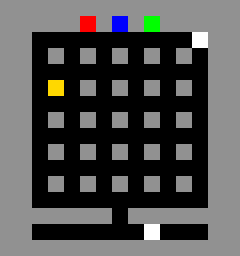
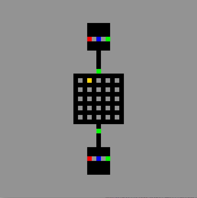
2) We empirically evaluate hysteretic and lenient approaches in two AFG layouts (Figure 2). Layout 1 examines whether the pathologies can be overcome when ILs can observe each other while making an irrevocable choice that determines the outcome of an episode. In contrast layout 2 requires ILs to independently make the same irrevocable decision in seclusion. We find that ILs predominately converge upon superior joint-policies in layout 1, providing evidence that ILs can implicitly learn to avoid miscoordination when able to observe each other during transitions that determine an episode’s outcome. Layout 2 poses a challenge for existing approaches. Lenient learners in particular face the following dilemma: remain lenient and be led astray by misleading stochastic rewards, or estimate average utility values and succumb to relative overgeneralisation due oscillating utility values caused by stochastic transitions.
3) We introduce NUI-DDQN, a MA-DRL algorithm which discards episodes yielding cumulative rewards outside the range of expanding intervals. These intervals are maintained for sequences of transitions (trajectories) equivalent to actions from cooperative games. NUI-DDQN reduces the noise introduced by punishing values resulting from miscoordination to utility estimates, allowing ILs to overcome relative overgeneralisation and the alter-exploration problem. NUI-DDQN consistently converges upon the optimal joint-policy in both layouts for deterministic and stochastic rewards.
2. Definitions and Notations
Below is a summary of the definitions used in this paper. Although many of the concepts discussed are from game theory we shall use the terms agent and player interchangeably. Furthermore, to prevent confusion we refer to actions taken in strategic-form games as while actions in Markov games are denoted as .
Strategic-Form Games. A strategic-form game is defined as a tuple where represents the number of agents, the joint action space , with being the set of actions available to agent , and is the reward function for each agent Bowling and Veloso (2002). In this paper, we focus on strategic-form games with , commonly known as bimatrix games. We note that in strategic-form games players make their choices simultaneously.
Stochastic rewards. Normally in a strategic-form game, all rewards are deterministic (DET). Given that stochasticity (of both rewards and transitions) are a central pathology of MA-RL, in this paper we also consider both partially stochastic (PS) and fully stochastic (FS) rewards. DET and FS reward functions exclusively return deterministic and stochastic rewards respectively for each . Meanwhile for a PS reward function there exists up to joint actions for which a stochastic reward is returned, while the remaining joint actions return deterministic rewards Wei and Luke (2016).
Markov Games. In contrast to strategic-form games where choices are made simultaneously, in a Markov game players make their choices sequentially. The game transitions from state to state, with choices and corresponding rewards collected along the way. Formally, a Markov game has a finite state space , an observation function which returns a -dimensional observation for agent , for each state a joint action space , with being the number of actions available to agent , a transition function , returning the probability of transitioning from a state to given an action profile , and a reward function: for each agent Shapley (1953); Leibo et al. (2017). We allow terminal states at which the game ends. Note that a strategic-form game can be thought of a Markov game with a single terminal state.
Policies. For agent , the policy represents a mapping from the observation space to a probability distribution over actions: , while refers to a joint policy of all agents. Joint policies excluding agent are defined as . The notation refers to a joint policy with agent following while the remaining agents follow .
Trajectories. We call a particular roll-out of a policy , i.e., the sequence of resulting states, actions, and associated rewards, a trajectory and denote it by Sutton et al. (1999).
Expected Gain. Given a joint policy the gain (or expected sum of future rewards) for each agent starting from a state is defined in Equation 1 below, where refers to the reward received by agent at time-step , while is a discount factor Matignon et al. (2012):
| (1) |
Nash Equilibrium. For a Markov game, a joint policy is a Nash equilibrium if and only if no agent can improve it’s gain through unilaterally deviating from Matignon et al. (2012):
| (2) |
Pareto Optimality. From a group perspective Nash equilibria are often sub-optimal. In contrast Pareto-optimality defines a joint policy from which no agent can deviate without making at least one other agent worse off. A joint policy is therefore Pareto-dominated by iff Matignon et al. (2012):
| (3) |
Pareto Dominated Nash Equilibrium. A joint policy is Pareto optimal if it is not Pareto-dominated by any other Matignon et al. (2012).
Team Games. A game, be it a strategic-form or Markov game, is a team game if every player gets the same reward, i.e., . Thus, team games are fully cooperative settings, where players have a shared objective to maximize their common return (see Figure 1) Claus and Boutilier (1998); Buşoniu et al. (2010); Matignon et al. (2012). In the rest of the paper, we only consider team games.
3. Temporally-extended Team Games
We conduct empirical evaluations in temporally-extended versions of team bimatrix games (TEGs). The outcome of these games is determined by joint-trajectories resulting from . The reward function has inequalities mirroring those of the corresponding bimatrix game. Therefore, each belongs to a set of trajectories that implements an action . ILs are tasked with learning a joint policy that results in optimal joint trajectories . Throughout this paper refers to a trajectory that consists of all the state-transition tuples of an individual episode. In Section 7, we introduce a temporally-extended version of the Climb Game, which serves as the basis for our experiments.
4. Pathologies in MA-RL
In this section, we elaborate on the pathologies outlined in the introduction. As mentioned, addressing one pathology often leaves agents vulnerable towards others. We discuss this in detail, while considering the implications of tackling these pathologies in complex environments. To understand the pathologies, we consider two types of ILs attempting to estimate the quality of an action when paired with the actions available to the other agent Wei and Luke (2016):
-
•
Average based learners estimate the quality of based on the average return: .
-
•
Maximum based learners estimate the quality of based on the maximum return observed: .
We now discuss the four pathologies: relative overgeneralisation, stochasticity, the alter-exploration, and moving target problems.
4.1. Relative Overgeneralisation
Relative overgeneralisation is a type of Action Shadowing, occurring in games where a sub-optimal Nash Equilibrium yields a higher payoff on average when each selected action is paired with an arbitrary action chosen by the other player Wei and Luke (2016). A shadowed equilibrium is an equilibrium defined by a policy that is shadowed by a policy in a state , where at least one agent exists who when unilaterally deviating from , will receive a gain less than the minimum gain that can be obtained for deviating from (Equation 4) Matignon et al. (2012). Relative overgeneralisation occurs in games where, as a result of a shadowed equilibrium, the agents converge upon a sub-optimal Nash Equilibrium that is Pareto-dominated by at least one other Nash Equilibrium Wei and Luke (2016); Matignon et al. (2012); Luke et al. (2008).
| (4) |
Example: Variations of the Climb Game Claus and Boutilier (1998) (Figure 1) are frequently used to study the susceptibility of ILs towards relative overgeneralisation. In the Climb Game the Pareto-Optimal Nash Equilibrium is . However, assuming two ILs initially choose each of the actions available with equal probability, using an average based algorithm, then Agent 1 will estimate that should be preferred over and , since and for each of Agent 2’s actions Wei and Luke (2016). Agent 2 will come to the same conclusion, resulting in the agents gravitating towards the shadow equilibrium . If an alternative action is still being played with a small probability, then Agent 1 will move from action to . Subsequently Agent 2 will also climb from to . At this point the agents will climb no further, having reached a Pareto dominated sub-optimal Nash equilibrium .
4.2. Stochasticity of rewards and transitions
In the deterministic reward Climb Game (Figure 1(a)) relative overgeneralisation can be overcome with maximum-based learning, where agents consider each action based on the observed Wei and Luke (2016). However, this approach leaves agents vulnerable towards misleading stochastic rewards. For example, in the Partially Stochastic Climb Game (Figure 1(b)) the joint action yields stochastic rewards of 14 and 0 with 50% probability. Therefore maximum based learners are drawn towards , despite each agent only receiving a reward of 7 on average. In temporally extended games additional stochasticity can emerge as a result of environmental factors such as noisy observations and probabilistic state transitions. Meanwhile, ILs facing the curse of dimensionality must overcome challenges introduced by noisy approximated utility estimates backed-up from stochastic follow-on state-transitions or rewards Matignon et al. (2012).
| Player 2 | ||||
| Player 1 | ||||
| Player 2 | ||||
| Player 1 | ||||
4.3. The alter-exploration problem
The exploration-exploitation trade-off required by reinforcement learners adds to the challenge of learning noise-free utility estimates. Matignon et al. Matignon
et al. (2012) define global exploration, the probability of at least one of agents exploring as , where each agent explores according to a probability . In environments with a shadowed equilibrium, as defined in Section 4.1, higher global exploration can result in agents converging upon a sub-optimal joint policy, as exploration can lead to penalties Matignon
et al. (2012). Furthermore, we consider that in TEGs agents face two types of alter-exploration:
1.) Exploring at an atomic level. Due to global exploration short sequences of actions may be sub-optimal, e.g., collisions with other agents, sub-optimal paths, etc, thereby introducing noise when the agents compute utility value estimates.
2.) Exploring at a trajectory level. Global exploration can impact the set of trajectories that trajectory belongs to for an agent , and therefore the outcome of an episode. We therefore argue that for MA-DRL algorithms to overcome the alter-exploration problem considerations are required at both levels.
4.4. The moving target problem
When multiple ILs update policies in parallel an environment can no longer be considered Markovian, thereby losing the property that guarantees convergence for a large number of single-agent learning algorithms Bowling and Veloso (2002); Sutton and Barto (1998). This problem is amplified in MA-DRL, where using ERMs often results in deprecated transitions being sampled during training Foerster et al. (2017); Omidshafiei et al. (2017); Palmer et al. (2018). Furthermore, as we shall discuss in section 8.5, stochastic transitions can lead to the moving target problem, which can result in long periods of miscoordination.
5. Independent Learner Baselines
The algorithms evaluated are extensions of the Double-DQN (DDQN) introduced by Van Hasselt et al. Van Hasselt et al. (2016). Each agent is implemented with a ConvNet trained to approximate Q-Values for observation-action pairs: Leibo et al. (2017). The network parameters are trained using Adam Kingma and Ba (2014) on the mean squared Bellman residual with the expectation taken over state transitions uniformly sampled from an ERM based on a probability distribution Mnih et al. (2015); Lin (1992),
| (5) |
where is the target:
| (6) |
The set of parameters in Equation 6 belong to a more stable target network, which is synchronised with the current network every transitions Van Hasselt et al. (2016). Each IL agent is implemented with a separate ERM used to store state transitions as tuples , consisting of an observation , action , the resulting observation and the immediate reward . To ensure obsolete transitions are eventually discarded ERMs are implemented as First-In First-Out (FIFO) queues Leibo et al. (2017).
5.1. Hysteretic Q-Learning
Hysteretic Q-Learning is an optimistic MA-RL algorithm originally introduced to address maximum based learner’s vulnerability towards stochasticity by using two learning rates and , where Wei and Luke (2016). Given a TD-Error , where , a hysteretic Q-value update is performed as described in Equation 7, where reduces the impact of negative Q-Value updates while learning rate is used for positive updates Matignon et al. (2007). However, hysteretic Q-Learners still have a tendency to gravitate towards sub-optimal policies when receiving misleading stochastic rewards Wei and Luke (2016); Palmer et al. (2018).
| (7) |
5.2. Leniency
Lenient learners have proven robust towards stochastic rewards by initially forgiving (ignoring) sub-optimal actions by teammates, while over time applying an average based approach for frequently visited observation-action pairs Panait et al. (2006, 2008); Zheng et al. (2018); Wei and Luke (2016); Palmer et al. (2018). The frequency with which negative updates are performed is determined by Equation 8 and a random variable , with negative updates only taking place if (Equation 9). Constant is a leniency moderation factor determining how the temperature value affects the drop-off in lenience Wei and Luke (2016). The temperature is decayed each time an pair is encountered. Meanwhile, Lenient-DDQNs (LDDQNs) store the leniency value computed at time inside the ERM, subsequently determining the frequency with which the corresponding transition can induce negative updates Palmer et al. (2018).
| (8) |
| (9) |
6. Negative Update Intervals in MA-DRL
Our aim is to compute intervals for each action , where the lower endpoint is approximately the reward received for coordinated behaviour involving . Therefore, receiving a reward less than on the interval indicates miscoordination has occurred. Below we define negative update intervals and describe how they help NUI-DDQN overcome relative overgeneralisation in TEGs.
Negative Updates. We define negative updates as Q-value updates using a TD-Error . In Equations 7 and 9 both leniency and hysteretic Q-learning reduce the impact of updates that would result in the lowering of Q-Values. However, neither algorithm distinguishes lowering Q-Values due to stochastic rewards from lowering based on miscoordination. Maximum based learners meanwhile avoid negative updates altogether by maintaining utility values for each action based on the highest observed reward .
Negative Update Intervals. While agents guided by are vulnerable towards stochastic rewards, we consider that for PS and FS reward spaces where for coordinated outcomes is greater than the punishment received for miscoordination, there exists intervals within which negative updates to utility estimates can be performed while mitigating the noise induced through punishment for miscoordination. We show that maintaining negative update intervals for each action increases the likelihood of agents within TEGs converging upon an optimal joint policy .
Classifying Trajectories. Joint-trajectories determine the rewards yielded by TEGs. Therefore, given an oracle capable of determining the set that trajectory belongs to, negative update intervals can be stored for each action , thereby increasing the likelihood of ILs computing noise free average utility values for transitions belonging to coordinated joint-trajectories . For simplicity our evaluations use TEGs with a predefined . However, under Future Work (Section 10) we discuss the potential of using a theory of mind neural network Rabinowitz et al. (2018) for .
Maintaining Negative Update Intervals. We establish for each action during an initial exploration phase used to fill the ERMs. Initially . During training is gradually decayed. To prevent a premature decay during phases where ILs are confronted with the alter-exploration problem,
we only only decay if the cumulative reward for the trajectory () is large enough.
That is, is only decayed if , where is a small constant.
Addressing Catastrophic Forgetting. Catastrophic forgetting occurs when trained networks forget how to perform previously learned tasks while learning to master a new task Goodfellow et al. (2013). To allow agents to maintain Q-Values for transitions belonging to less frequently observed actions , without preventing outdated transitions from being discarded, we implement a separate ERM for each action . Instead of storing transitions each stores episodes, since traditional ERMs may store a significant number of obsolete transitions once ILs become efficient at solving a task and require less steps. Episodic ERMs meanwhile are more likely to reflect the current search space. During sampling the are concatenated.
Storing Trajectories. In addition to we maintain vectors , which store the most recent cumulative rewards for each action . A trajectory is stored iff the cumulative reward is greater than the max between and the ’s mean minus the standard deviation (Equation 10). Therefore, while leniency is vulnerable towards miscoordination upon cooling temperature values, NUI-DDQN will continue to discard miscoordination trajectories.
| (10) |
7. The Apprentice Firemen Game (AFG)
The Climb Game is often studied as a repeated game. We are interested in solving an equivalent game extended over the temporal dimension, where joint trajectories result in outcomes comparable to the joint-actions from Figure 1. We formulate a TEG based on the Climb Game that we call the Apprentice Firemen Game (AFG), where two (or more) agents located within a gridworld are tasked with locating and extinguishing fires. First however the agents must locate an equipment pickup area and choose one of the items listed in Table 1 below. The task is fully cooperative, i.e. both agents are required to extinguish one fire. As outlined in Table 1 both agents detonating an explosive device (fighting fire with fire) is the most effective combination, equivalent to the joint action in the Climb Game. While the fire extinguisher is more effective than the fire blanket, agents choosing one run the risk of being hit by debris if the other agent triggers an explosive device, whereas the fire blanket offers protection. Therefore the fire extinguisher and fire blanket are equivalent to actions and respectively.
| Description | Action () | Effectiveness | Risk |
| Explosive Device | A | High | High |
| Fire Extinguisher | B | Medium | High |
| Fire Blanket | C | Weak | None |
ILs are not explicitly told which actions other agents have performed Wei and Luke (2016). However, we hypothesize ILs can learn to avoid miscoordination in the AFG when able to observe each other during transitions that determine an episode’s outcome, reducing the impact of optimal joint action being a shadowed equilibrium. To test this hypothesis we conduct experiments using two layouts outlined below (and illustrated in Figure 2), where equipment pickup decisions are irrevocable for the duration of each episode. At the start of an episode one randomly chosen obstacle in the main area is set on fire. Episodes end when both agents occupy cells next to the fire, upon which a terminal reward is returned. To eliminate confounding factors all non-terminal transitions yield a reward of 0. We introduce a 10,000 step limit upon observing that trained agents delay miscoordination outcomes through avoiding the fire. The agents receive a miscoordination reward of -1.0 upon reaching this limit. The action space is discrete and includes moving up, down, left, right and NOOP. Pickup actions occur automatically upon ILs entering an equipment cell empty handed. DDQNs perform well when receiving rewards within , which led us to choose the reward structures listed in Figure 3. For stochastic transitions randomly moving civilians can be added who obstruct paths.
Layout 1: Observable irrevocable decisions Two agents in a gridworld begin each episode in opposite corners of a compartment separated from the main area. The agents must exit the compartment, gather equipment from a shared pickup area and subsequently extinguish the fire, meaning that agents observe each other during the irrevocable equipment selection process. One agent can therefore observe the other agent’s choice and subsequently select a best response to avoid miscoordination - in terms of the original Climb (bimatrix) game, this allows agents to act as if it was a perfect-information commitment version of the game with a follower and leader.
Layout 2: Irrevocable decisions in seclusion Two agents in a padded gridworld begin each episode in separate chambers. To mimic the simultaneity of the choice of actions in the Climb (bimatrix) game, each agent is limited to centered observations. Agents are therefore unable to observe each others’ equipment selection actions.
| Deterministic (DET) | Partially Stochastic (PS) | Fully Stochastic (FS) | |||||||
| Action | A | B | C | A | B | C | A | B | C |
| A | |||||||||
| B | * | * | |||||||
| C | |||||||||
8. Empirical Evaluation
8.1. MA-DRL implementation details
Given the number of cells within the main area that agents can occupy (90), fire locations (25), agent color combinations (16) and actions (5) we estimate 16,020,000 state-action pairs per layout before factoring in civilians and additional layout specific cells. We therefore follow the example of recent publications by conducting evaluations in gridworlds with sufficient complexity to warrant a MA-DRL approach Leibo et al. (2017); Gupta et al. (2017); Palmer et al. (2018). Networks consist of 2 convolutional layers with 32 and 64 kernels respectively, a fully connected layer (1024 neurons) and an output node for each action111We make our code available online: https://github.com/gjp1203/nui_in_madrl. We use learning rate , discount rate and -Greedy exploration with a decay rate of 0.999. Each stores 250,000 transitions. Regarding algorithm specific configurations:
NUI-DDQN. To determine the set of trajectories that belongs to each oracle queries the respective agent instance regarding the ID of the equipment used. Each stores 100 episodes, while the decay rate for is set to 0.995.
LDDQNs. We use a leniency moderation factor and a retroactive temperature decay schedule combined with temperature greedy exploration strategy as described in Palmer et al. (2018).
HDDQNs. In our evaluation below is the decimal portion of .
8.2. Experiments
To evaluate our hypothesis in Section 7 we collect 30 training runs of 5,000 episodes per algorithm within each layout. For LDDQNs an additional 5,000 episodes are required to sufficiently decay the temperatures . Finally, to evaluate the impact of stochastic transitions we introduce 10 civilians in layout 2 and conduct 30 runs of 10,000 episodes per setting.
8.3. Evaluation using phase plots
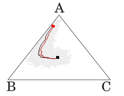
The ternary phase plots depicted in Table 2 provide insights regarding the learning dynamics of the agents. Each line illustrates the average shift in the trajectory distributions throughout the runs conducted, using a rolling window of 1000 episodes. The black squares at the centre of each plot represent the averaged initial distributions while the red dots represents the final distribution. Each corner represents 100% of trajectories for the labelled action . For example, if both lines end with red dots in the top corner of a simplex, then the two agents are predominately producing trajectories , and have converged upon the optimal Nash Equilibrium . The agents have therefore learned policies where the optimal equipment is being selected from the pickup area in the AFG, as outlined in section 7.
Determistic rewards. Under pathologies (Section 4) we discuss how maximum based learners can overcome relative overgeneralisation in the deterministic reward Climb Game. Similarly the phase plots for deterministic reward settings confirm that with sufficient optimism / leniency, ILs can overcome relative overgeneralisation while facing the curse of dimensionality (HDDQN , LDDQN and NUI-DDQN in Table 2). Meanwhile, HDDQN shows that agents with insufficient optimism gravitate towards the shadow equilibrium . Interestingly in layout 2 with 10 civilians HDDQN agents are completing the climb steps discussed in Section 4.1 towards , while converge towards superior joint policies compared to layout 2 without civilians. Further investigation is required to establish why.
Stochastic Rewards. As evident by the phase plots in Table 2 the optimism that helps HDDQNs overcome relative overgeneralisation in the deterministic reward settings can lead agents to converge upon sub-optimal joint policies when learning from PS or FS rewards. For HDDQN for instance we observe an increase in for PS, and by agent 2 for FS rewards. LDDQNs meanwhile are less vulnerable, gravitating towards optimal joint-policies despite stochastic rewards and relative overgeneralisation in layout 1 and when receiving PS rewards in layout 2 with no civilians. However, LDDQNs struggle when receiving FS rewards in layout 2, and have limited success once civilians are added. NUI-DDQNs meanwhile predominately converge upon optimal joint-policies. When receiving PS rewards NUI-DDQNs are initially tempted by the misleading rewards received for , before converging on a joint-policy with the majority of trajectories . For FS rewards a slight increase in can be observed.
| Layout 1 (Civilians: 0, Episodes: 5,000) | Layout 2 (Civilians: 0, Episodes: 5,000) | Layout 2 (Civilians: 10, Episodes: 10,000) | ||||||
| DET | PS | FS | DET | PS | FS | DET | PS | FS |
| Hysteretic-DDQN =0.5 | ||||||||
![[Uncaptioned image]](/html/1809.05096/assets/V30C/HDDQN_05_2A_0C_DET_V3.png) |
![[Uncaptioned image]](/html/1809.05096/assets/V30C/HDDQN_05_2A_0C_PS_V3.png) |
![[Uncaptioned image]](/html/1809.05096/assets/V30C/HDDQN_05_2A_0C_FS_V3.png) |
![[Uncaptioned image]](/html/1809.05096/assets/V20C/HDDQN_05_2A_0C_DET_V2.png) |
![[Uncaptioned image]](/html/1809.05096/assets/V20C/HDDQN_05_2A_0C_PS_V2.png) |
![[Uncaptioned image]](/html/1809.05096/assets/V20C/HDDQN_05_2A_0C_FS_V2.png) |
![[Uncaptioned image]](/html/1809.05096/assets/V210C/HDQN05_DET_2A_10C.png) |
![[Uncaptioned image]](/html/1809.05096/assets/V210C/HDQN05_PS_2A_10C.png) |
![[Uncaptioned image]](/html/1809.05096/assets/V210C/HDQN05_FS_2A_10C.png) |
| Hysteretic-DDQN =0.7 | ||||||||
![[Uncaptioned image]](/html/1809.05096/assets/V30C/HDDQN_07_2A_0C_DET_V3.png) |
![[Uncaptioned image]](/html/1809.05096/assets/V30C/HDDQN_07_2A_0C_PS_V3.png) |
![[Uncaptioned image]](/html/1809.05096/assets/V30C/HDDQN_07_2A_0C_FS_V3.png) |
![[Uncaptioned image]](/html/1809.05096/assets/V20C/HDDQN_07_2A_0C_DET_V2.png) |
![[Uncaptioned image]](/html/1809.05096/assets/V20C/HDDQN_07_2A_0C_PS_V2.png) |
![[Uncaptioned image]](/html/1809.05096/assets/V20C/HDDQN_07_2A_0C_FS_V2.png) |
![[Uncaptioned image]](/html/1809.05096/assets/V210C/HDQN07_DET_2A_10C.png) |
![[Uncaptioned image]](/html/1809.05096/assets/V210C/HDQN07_PS_2A_10C.png) |
![[Uncaptioned image]](/html/1809.05096/assets/V210C/HDQN07_FS_2A_10C.png) |
| Hysteretic-DDQN =0.9 | ||||||||
![[Uncaptioned image]](/html/1809.05096/assets/V30C/HDDQN_09_2A_0C_DET_V3.png) |
![[Uncaptioned image]](/html/1809.05096/assets/V30C/HDDQN_09_2A_0C_PS_V3.png) |
![[Uncaptioned image]](/html/1809.05096/assets/V30C/HDDQN_09_2A_0C_FS_V3.png) |
![[Uncaptioned image]](/html/1809.05096/assets/V20C/HDDQN_09_2A_0C_DET_V2.png) |
![[Uncaptioned image]](/html/1809.05096/assets/V20C/HDDQN_09_2A_0C_PS_V2.png) |
![[Uncaptioned image]](/html/1809.05096/assets/V20C/HDDQN_09_2A_0C_FS_V2.png) |
![[Uncaptioned image]](/html/1809.05096/assets/V210C/HDQN09_DET_2A_10C.png) |
![[Uncaptioned image]](/html/1809.05096/assets/V210C/HDQN09_PS_2A_10C.png) |
![[Uncaptioned image]](/html/1809.05096/assets/V210C/HDQN09_FS_2A_10C.png) |
| Lenient-DDQN | ||||||||
![[Uncaptioned image]](/html/1809.05096/assets/V30C/LDDQN_2A_0C_DET_V3.png) |
![[Uncaptioned image]](/html/1809.05096/assets/V30C/LDDQN_2A_0C_PS_V3.png) |
![[Uncaptioned image]](/html/1809.05096/assets/V30C/LDDQN_2A_0C_FS_V3.png) |
![[Uncaptioned image]](/html/1809.05096/assets/V20C/LDDQN_2A_0C_DET_V2.png) |
![[Uncaptioned image]](/html/1809.05096/assets/V20C/LDDQN_2A_0C_PS_V2.png) |
![[Uncaptioned image]](/html/1809.05096/assets/V20C/LDDQN_2A_0C_FS_V2.png) |
![[Uncaptioned image]](/html/1809.05096/assets/V210C/LDDQN_2A_10C_DET_V2.png) |
![[Uncaptioned image]](/html/1809.05096/assets/V210C/LDDQN_2A_10C_PS_V2.png) |
![[Uncaptioned image]](/html/1809.05096/assets/V210C/LDDQN_2A_10C_FS_V2.png) |
| NUI-DDQN | ||||||||
![[Uncaptioned image]](/html/1809.05096/assets/V30C/NUIDDQN_2A_0C_DET_V3.png) |
![[Uncaptioned image]](/html/1809.05096/assets/V30C/NUIDDQN_2A_0C_PS_V3.png) |
![[Uncaptioned image]](/html/1809.05096/assets/V30C/NUIDDQN_2A_0C_FS_V3.png) |
![[Uncaptioned image]](/html/1809.05096/assets/V20C/2A_0C_DET.png) |
![[Uncaptioned image]](/html/1809.05096/assets/V20C/2A_0C_PS.png) |
![[Uncaptioned image]](/html/1809.05096/assets/V20C/2A_0C_FS.png) |
![[Uncaptioned image]](/html/1809.05096/assets/V210C/2A_10C_DET.png) |
![[Uncaptioned image]](/html/1809.05096/assets/V210C/2A_10C_PS.png) |
![[Uncaptioned image]](/html/1809.05096/assets/V210C/2A_10C_FS.png) |
|
|
||||||||
8.4. Learning best response policies
In Section 7 we proposed that ILs should learn to avoid miscoordination trajectories within layout 1 due to observing each other during interactions with the equipment pick-up area. To compare the policies learned in layouts 1 and 2 (without civilians), we compute the average coordinated rewards for each training run. We compute using the rewards from the final 1000 episodes that did not end in miscoordination outcomes . Runs with have converged upon the optimal joint-policy, where is the most frequently observed outcome. For the majority of settings higher values are achieved by agents in layout 1. The scatter plots in Table 3 provide evidence to support our hypothesis. Each marker within the scatter plots represents the for an individual run. To provide further clarity we sort the runs by . We observe that HDDQN and converges upon a policy with numerous times in each reward setting in layout 1, while only twice in layout 2 (HDDQN , PS & FS) 222We provide additional scatter plots for each evaluation setting in the Appendix.. Interestingly we find that for HDDQN (, PS) and LDDQN (DET & PS) a larger number of runs converge upon joint-policies where in layout 2. NUI-DDQNs meanwhile perform consistently when receiving deterministic and partially stochastic rewards in both settings, while a couple of runs faltered for fully stochastic rewards within layout 2. It is worth noting that even for NUI-DDQN runs with low , remains a frequently observed outcome.
| Deterministic | Partially Stochastic | Fully Stochastic |
| HDQN | ||
![[Uncaptioned image]](/html/1809.05096/assets/SCATTER/HDQN07_DET.png) |
![[Uncaptioned image]](/html/1809.05096/assets/SCATTER/HDQN07_PS.png) |
![[Uncaptioned image]](/html/1809.05096/assets/SCATTER/HDQN07_FS.png) |
| HDQN | ||
![[Uncaptioned image]](/html/1809.05096/assets/SCATTER/HDQN09_DET.png) |
![[Uncaptioned image]](/html/1809.05096/assets/SCATTER/HDQN09_PS.png) |
![[Uncaptioned image]](/html/1809.05096/assets/SCATTER/HDQN09_FS.png) |
8.5. Impact of stochastic transitions
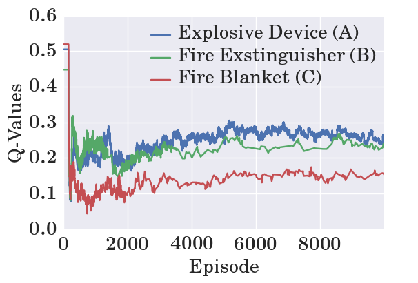
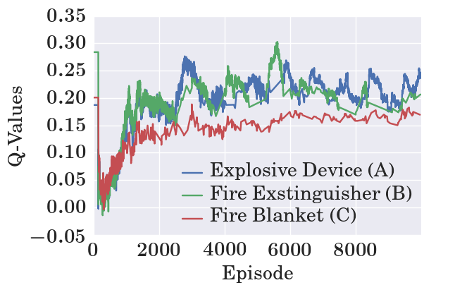
Introducing 10 civilians to layout 2 allows us to examine the challenges faced by MA-DRL agents when attempting to overcome relative overgeneralisation while making decisions using noisy utility values backed up from stochastic follow-on transitions. In Figure 4 we compare the Q-Values from actions leading to the selection of equipment within both 0 and 10 civilian settings from two individual NUI-DDQN runs with PS rewards. We observe that Q-Values oscillate significantly upon introducing civilians, with Q-Values belonging to sub-optimal equipment pickups frequently rising above those belonging to . Stochastic transitions can therefore lead to the moving target problem (Section 4.4), in this case resulting in extended periods of miscoordination. However, by maintaining negative update intervals, NUI-DDQN can overcome miscoordination and revert back to a policy that generates trajectories .
8.6. Considerations regarding LDDQNs
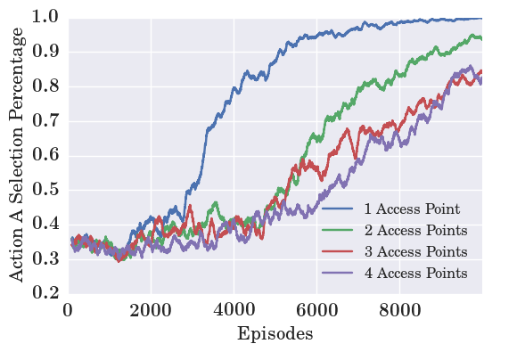
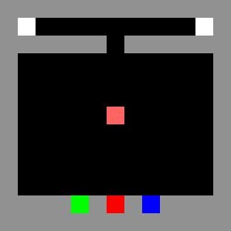
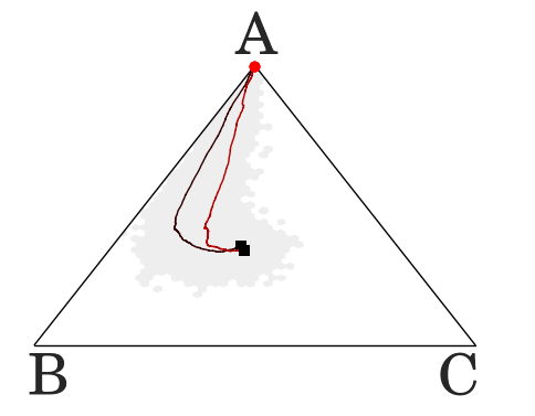
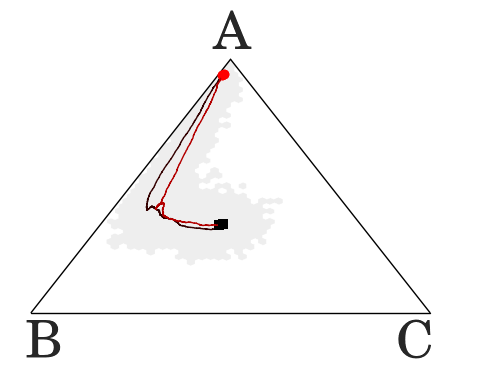
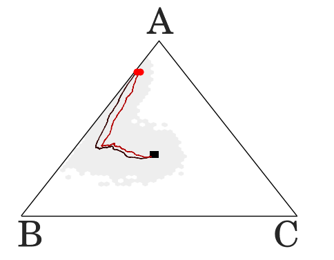
The phase plots in Table 2 indicate that given more time an increase in trajectories should be possible for LDDQNs. However, while searching for an optimal set of hyperparameters we became aware of one particular dilemma: while LDDQNs fail to converge upon with insufficiently decayed temperature values, rapidly decaying temperature values leaves LDDQNs vulnerable during the periods of miscoordination discussed in Section 8.5. We therefore choose a patient approach, with the consequence that even after 10,000 episodes the agents have still not converged. To illustrate this dilemma we conduct additional runs in a simplified PS reward version of layout 1 with only 1 fire location. By varying the number of obstacles surrounding this fire, and thereby controlling the number of Access Points from which the agents can extinguish it, we observe the rolling percentage of outcomes increases significantly faster when the number of values that need decaying decreases. We conduct 20 runs for each access point setting:
9. Related Literature
ILs within MA-DRL systems are receiving an increasing amount of attention within literature. However, a lot of this research focuses on the impact of stochasticity and the amplified moving target problem caused by ERMs Hernandez-Leal et al. (2018). Zheng et al. Zheng et al. (2018) introduce a Weighted Double-DQN that makes use of a lenient reward network along with a scheduled replay strategy to improve the convergence rate within stochastic cooperative environments. Foerster et al. Foerster et al. (2017) show that the ERM can be stabilised by using importance sampling as a means to identify outdated state transitions by maintaining observation histories of the actions taken by the other agents in the system. A further active area within MA-DRL research is centralized training for decentralized execution. Gupta et al. Gupta et al. (2017) evaluate policy gradient, temporal difference error, and actor critic methods on cooperative control tasks that include discrete and continuous state and action spaces, using a decentralized parameter sharing approach with centralized learning. Rashid et al. Rashid et al. (2018) propose QMIX, introducing a network that estimates joint action-values as a non-linear combination of agent-values, thereby helping agents learn optimal joint-action values based on the additional information that centralized learning provides. Perhaps the most relevant recent work to our research is by Wei et al. Wei et al. (2018), who introduce Multiagent Soft Q-Learning, an algorithm which converges towards a superior local optima compared to MA-DDPG Lowe et al. (2017) within continuous action domains suffering from relative overgeneralisation. In contrast to our approach Multiagent Soft Q-Learning augments rewards with an entropy term, thereby increasing the likelihood of finding multiple modes within a continuous action space compared to the discrete action space used in our experiments Wei et al. (2018); Haarnoja et al. (2017). However, Multiagent Soft Q-Learning is currently a centralized approach that has only been tested within a single state continuous game for two agents, with the authors currently investigating the algorithm’s scalability to ILs within sequential continuous games.
10. Future work
1) We conducted trials using 20 sets of fixed policies trained in a simplified layout 1, finding evidence that leader-follower dynamics emerge during training, where one agent waits to observe the other’s equipment choice. We assigned the policies to disjoint sets and based on the percentage of and their roll-outs produced. Upon subsequently running trials with each leader-follower combination, we find half of followers choose when paired with a leader and vice-versa. We are currently investigating why only some ILs develop this adaptive ability.
2) For simplicity, the actions returned by the oracle for the AFG are predefined. Going foward, recent work on the topic of theory of mind by Rabinowitz et al. Rabinowitz et al. (2018) could pave the way for a learned oracle . The authors build a data-efficient meta-learner that learns models of the agents that it encounters. Through observing trajectories their resulting theory of mind network architecture is used to predict next-step actions, the consumption of objects within the environment and the successor representation. This opens up the possibility of applying NUI-DDQN to more complex domains where a learning approach is required to identify actions .
11. Conclusions
Our empirical evaluation highlights the challenges MA-DRL agents must overcome, to avoid converging upon sub-optimal joint policies when making decisions using noisy approximated utility estimates backed-up from stochastic follow-on state-transitions and rewards.
To summarize our contributions:
1) We presented the Apprentice Firemen Game (AFG), which is a new and challenging environment that simultaneously confronts learners with four pathologies: relative overgeneralisation, stochasticity, the moving target problem, and alter exploration problem.
2) We evaluate hysteretic Omidshafiei et al. (2017) and lenient Palmer
et al. (2018) learners on the AFG. While both approaches can overcome the pathologies in simpler settings, they fail when required to independently make irrevocable decisions in seclusion determining an episode’s outcome.
3) Motivated by this we designed a new algorithm NUI-DDQN that is based on negative update intervals. Our algorithm identifies and discards episodes that end in miscoordination. In doing so, it reduces the noise introduced by the large punishments that result from miscoordination. We show that NUI-DDQN consistently converges towards the optimal joint-policy within each setting.
12. Acknowledgments
We thank the HAL Allergy Group for partially funding the PhD of Gregory Palmer and gratefully acknowledge the support of NVIDIA Corporation with the donation of the Titan X Pascal GPU that enabled this research.
References
- (1)
- Bowling and Veloso (2002) Michael Bowling and Manuela Veloso. 2002. Multiagent learning using a variable learning rate. Artificial Intelligence 136, 2 (2002), 215–250.
- Buşoniu et al. (2010) Lucian Buşoniu, Robert Babuška, and Bart De Schutter. 2010. Multi-agent reinforcement learning: An overview. In Innovations in multi-agent systems and applications-1. Springer, 183–221.
- Claus and Boutilier (1998) Caroline Claus and Craig Boutilier. 1998. The dynamics of reinforcement learning in cooperative multiagent systems. In AAAI/IAAI 1998 (1998), 746–752.
- Foerster et al. (2017) Jakob Foerster, Nantas Nardelli, Gregory Farquhar, Triantafyllos Afouras, Philip HS Torr, Pushmeet Kohli, and Shimon Whiteson. 2017. Stabilising Experience Replay for Deep Multi-Agent Reinforcement Learning. In Proc. of ICML. 1146–1155.
- Fulda and Ventura (2007) Nancy Fulda and Dan Ventura. 2007. Predicting and Preventing Coordination Problems in Cooperative Q-learning Systems. In IJCAI, Vol. 2007. 780–785.
- Goodfellow et al. (2013) Ian J Goodfellow, Mehdi Mirza, Da Xiao, Aaron Courville, and Yoshua Bengio. 2013. An empirical investigation of catastrophic forgetting in gradient-based neural networks. arXiv preprint arXiv:1312.6211 (2013).
- Gupta et al. (2017) Jayesh K Gupta, Maxim Egorov, and Mykel Kochenderfer. 2017. Cooperative Multi-Agent Control Using Deep Reinforcement Learning. In Proceedings of the Adaptive and Learning Agents workshop (at AAMAS 2017).
- Haarnoja et al. (2017) Tuomas Haarnoja, Haoran Tang, Pieter Abbeel, and Sergey Levine. 2017. Reinforcement learning with deep energy-based policies. arXiv preprint arXiv:1702.08165 (2017).
- Hernandez-Leal et al. (2018) Pablo Hernandez-Leal, Bilal Kartal, and Matthew E Taylor. 2018. Is multiagent deep reinforcement learning the answer or the question? A brief survey. arXiv preprint arXiv:1810.05587 (2018).
- Kingma and Ba (2014) Diederik P. Kingma and Jimmy Ba. 2014. Adam: A Method for Stochastic Optimization. In Proc. of ICLR.
- Leibo et al. (2017) Joel Z Leibo, Vinicius Zambaldi, Marc Lanctot, Janusz Marecki, and Thore Graepel. 2017. Multi-agent reinforcement learning in sequential social dilemmas. In Proc. of AAMAS. 464–473.
- Lin (1992) Long-H Lin. 1992. Self-improving reactive agents based on reinforcement learning, planning and teaching. Machine learning 8, 3/4 (1992), 69–97.
- Lowe et al. (2017) Ryan Lowe, Yi Wu, Aviv Tamar, Jean Harb, OpenAI Pieter Abbeel, and Igor Mordatch. 2017. Multi-agent actor-critic for mixed cooperative-competitive environments. In Proc. of NIPS. 6379–6390.
- Luke et al. (2008) Sean Luke, Liviu Panait, and Karl Tuyls. 2008. Theoretical advantages of lenient learners: An evolutionary game theoretic perspective. JMLR 9 (2008), 423–457.
- Matignon et al. (2007) Laëtitia Matignon, Guillaume Laurent, and Nadine Le Fort-Piat. 2007. Hysteretic Q-Learning: an algorithm for decentralized reinforcement learning in cooperative multi-agent teams. In Proc. of IROS. 64–69.
- Matignon et al. (2012) Laetitia Matignon, Guillaume J Laurent, and Nadine Le Fort-Piat. 2012. Independent reinforcement learners in cooperative Markov games: a survey regarding coordination problems. The Knowledge Engineering Review 27, 1 (2012), 1–31.
- Mnih et al. (2015) Volodymyr Mnih, Koray Kavukcuoglu, David Silver, Andrei A Rusu, Joel Veness, Marc G Bellemare, Alex Graves, Martin Riedmiller, Andreas K Fidjeland, Georg Ostrovski, et al. 2015. Human-level control through deep reinforcement learning. Nature 518, 7540 (2015), 529–533.
- Omidshafiei et al. (2017) Shayegan Omidshafiei, Jason Pazis, Christopher Amato, Jonathan P. How, and John Vian. 2017. Deep Decentralized Multi-task Multi-Agent Reinforcement Learning under Partial Observability. Proc. of ICML 70 (2017), 2681–2690.
- Palmer et al. (2018) Gregory Palmer, Karl Tuyls, Daan Bloembergen, and Rahul Savani. 2018. Lenient multi-agent deep reinforcement learning. In Proc. of AAMAS. 443–451.
- Panait et al. (2006) Liviu Panait, Keith Sullivan, and Sean Luke. 2006. Lenience towards teammates helps in cooperative multiagent learning. In Proc. of AAMAS.
- Panait et al. (2008) Liviu Panait, Karl Tuyls, and Sean Luke. 2008. Theoretical advantages of lenient learners: An evolutionary game theoretic perspective. JMLR 9, Mar (2008), 423–457.
- Rabinowitz et al. (2018) Neil Rabinowitz, Frank Perbet, Francis Song, Chiyuan Zhang, S. M. Ali Eslami, and Matthew Botvinick. 2018. Machine Theory of Mind. In Proc. of ICML, Jennifer Dy and Andreas Krause (Eds.), Vol. 80. PMLR, 4218–4227.
- Rashid et al. (2018) Tabish Rashid, Mikayel Samvelyan, Christian Schroeder de Witt, Gregory Farquhar, Jakob Foerster, and Shimon Whiteson. 2018. QMIX: Monotonic Value Function Factorisation for Deep Multi-Agent Reinforcement Learning. arXiv preprint arXiv:1803.11485 (2018).
- Shapley (1953) Lloyd S Shapley. 1953. Stochastic games. Proceedings of the national academy of sciences 39, 10 (1953), 1095–1100.
- Sutton and Barto (1998) Richard S Sutton and Andrew G Barto. 1998. Introduction to reinforcement learning. Vol. 135. MIT press Cambridge.
- Sutton et al. (1999) Richard S Sutton, Doina Precup, and Satinder Singh. 1999. Between MDPs and semi-MDPs: A framework for temporal abstraction in reinforcement learning. Artificial intelligence 112, 1-2 (1999), 181–211.
- Van Hasselt et al. (2016) Hado Van Hasselt, Arthur Guez, and David Silver. 2016. Deep Reinforcement Learning with Double Q-Learning. AAAI (2016), 2094–2100.
- Wei and Luke (2016) Ermo Wei and Sean Luke. 2016. Lenient Learning in Independent-Learner Stochastic Cooperative Games. JMLR 17, 84 (2016), 1–42.
- Wei et al. (2018) Ermo Wei, Drew Wicke, David Freelan, and Sean Luke. 2018. Multiagent Soft Q-Learning. arXiv preprint arXiv:1804.09817 (2018).
- Zheng et al. (2018) Yan Zheng, Zhaopeng Meng, Jianye Hao, and Zongzhang Zhang. 2018. Weighted Double Deep Multiagent Reinforcement Learning in Stochastic Cooperative Environments. In Pacific Rim International Conference on Artificial Intelligence. 421–429.
Appendix A Appendices
A.1. Hyperparameters
Table 4 lists the hyperparameters used for our empirical evaluation. To reduce the time required to evaluate LDDQN we apply python’s xxhash to masked observations (i.e., removing civilians).
| Component | Hyperparameter | Range of values |
| DDQN Base | Learning rate | 0.0001 |
| Discount rate | 0.95 | |
| Target network sync. steps | 5000 | |
| ERM Size | 250’000 | |
| -Greedy Exploration | Initial value | 1.0 |
| Decay factor | 0.999 | |
| Minimum Value | 0.05 | |
| Leniency | MaxTemperature | 1.0 |
| Leniency Modification Coefficient | 1.0 | |
| TDS Exponent | -0.1 | |
| TDS Exponent Decay Rate | 0.95 | |
| Initial Max Temperature Value | 1.0 | |
| Max Temperature Decay Coefficient | 0.9998 | |
| Action Selection Exponent | 0.25 | |
| Hashing | xxhash | |
| NUI-DDQN | Capacity | 100 Episodes |
| Decay threshold | 50 Episodes | |
| decay rate | 0.995 |
A.2. Learning Best Response Policies
Table 5 provides additional scatter plots for each evaluation setting. Each marker within the scatter plots represents the for an individual run. To provide further clarity we sort the runs by . We observe that for the majority of settings higher values are achieved by agents in layout 1. Interestingly only HDDQN (, PS Rewards) and LDDQN (DET & PS Rewards) achieved higher values in layout 2. NUI-DDQNs meanwhile perform consistently when receiving deterministic and PS rewards, while a couple of runs faltered for FS rewards within layout 2. It is worth noting that even for NUI-DDQN runs with low , remains a frequently observed outcome:
| HDQN () | HDQN () | HDQN () | LDDQN | NUI-DDQN | |
![[Uncaptioned image]](/html/1809.05096/assets/SCATTER/HDQN05_DET.png) |
![[Uncaptioned image]](/html/1809.05096/assets/SCATTER/HDQN07_DET.png) |
![[Uncaptioned image]](/html/1809.05096/assets/SCATTER/HDQN09_DET.png) |
![[Uncaptioned image]](/html/1809.05096/assets/SCATTER/LDDQN_DET.png) |
![[Uncaptioned image]](/html/1809.05096/assets/SCATTER/NUIDDQN_DET.png) |
DET |
![[Uncaptioned image]](/html/1809.05096/assets/SCATTER/HDQN05_PS.png) |
![[Uncaptioned image]](/html/1809.05096/assets/SCATTER/HDQN07_PS.png) |
![[Uncaptioned image]](/html/1809.05096/assets/SCATTER/HDQN09_PS.png) |
![[Uncaptioned image]](/html/1809.05096/assets/SCATTER/LDDQN_PS.png) |
![[Uncaptioned image]](/html/1809.05096/assets/SCATTER/NUIDDQN_PS.png) |
PS |
![[Uncaptioned image]](/html/1809.05096/assets/SCATTER/HDQN05_FS.png) |
![[Uncaptioned image]](/html/1809.05096/assets/SCATTER/HDQN07_FS.png) |
![[Uncaptioned image]](/html/1809.05096/assets/SCATTER/HDQN09_FS.png) |
![[Uncaptioned image]](/html/1809.05096/assets/SCATTER/LDDQN_FS.png) |
![[Uncaptioned image]](/html/1809.05096/assets/SCATTER/NUIDDQN_FS.png) |
FS |
A.3. LDDQN Variable Access Points Experiments: Layouts & Phase Plots
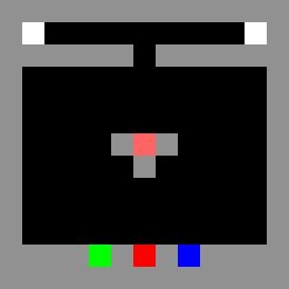
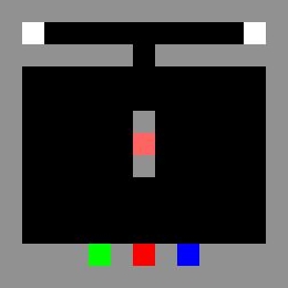
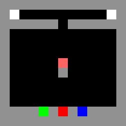
Figure 6 illustrates the AFG layouts used for the evaluations discussed in Section 8.6. We also provide the resulting phase plot for each layout.
of increasing the number of possible state-action pairs.