Simulated Tempering Method in the Infinite Switch Limit with Adaptive Weight Learning

Abstract

We investigate the theoretical foundations of the simulated tempering (ST) method and use our findings to design an efficient accelerated sampling algorithm. Employing a large deviation argument first used for replica exchange molecular dynamics [Nuria et al. J. Chem. Phys. 135:134111 (2011)], we demonstrate that the most efficient approach to simulated tempering is to vary the temperature infinitely rapidly. In this limit, we can replace the equations of motion for the temperature and physical variables by averaged equations for the latter alone, with the forces rescaled according to a position-dependent function defined in terms of temperature weights. The averaged equations are similar to those used in Gao’s integrated-over-temperature method, except that we show that it is better to use a continuous rather than a discrete set of temperatures. We give a theoretical argument for the choice of the temperature weights as the reciprocal partition function, thereby relating simulated tempering to Wang-Landau sampling. Finally, we describe a self-consistent algorithm for simultaneously sampling the canonical ensemble and learning the weights during simulation. This infinite switch simulated tempering (ISST) algorithm is tested on three examples of increasing complexity: a system of harmonic oscillators; a continuous variant of the Curie-Weiss model, where ISST is shown to perform better than standard ST and to accurately capture the second-order phase transition observed in this model; and Alanine-12 in vacuum, where ISST also compares favorably with standard ST in its ability to calculate the free energy profiles of the root mean square deviation (RMSD) and radius of gyration of the molecule in the 300-500K tempearture range.

Keywords high-dimensional sampling, molecular dynamics, simulated tempering, replica exchange, Wang-Landau method

1 Introduction

The sampling of probability distributions in high dimensions is a fundamental challenge in computational science, with broad applications to physics, chemistry, biology, finance, machine learning, and other areas (e.g. [1, 2, 3, 4]). The methods of choice to tackle this problem are based on Monte Carlo or the simulation of stochastic differential equations such as the Langevin equation, either of which can be designed to be ergodic for a wide class of probability distributions. Yet, straightforward application of these methods typically fails when the distribution displays complex features such as multimodality. In high dimensions, the per-step cost of generating samples is significant and can be taken as the unit of computational effort; naive approaches may require many millions or billions of iterations. A typical case in point arises in computational chemistry, where molecular dynamics (MD) simulation has become an invaluable tool for resolving chemical structures, exploring the conformational states of biomolecules and computing free energies. Yet, despite its versatility, the use of MD simulation is often limited by the intrinsic high dimensionality of the systems involved and the presence of entropic and energetic barriers which lead to slow diffusion and necessitate the use of very long trajectories. A typical MD simulation is thus spent oversampling a few free energy minima, with consequent poor approximation of properties of interest.

Numerous methods have been introduced for overcoming the intrinsic complexities of high-dimensional sampling. These accelerated sampling method include the Wang-Landau method [5, 6] which directly estimates the density of states and thus the entropy during simulation; metadynamics [7, 8] which progressively modifies the potential energy during simulation to flatten out the landscape and accelerate transitions between states; temperature-accelerated molecular dynamics (TAMD) [9, 10], which effectively evolves collective variables on their free energy landscape at the physical temperature but use an artificially high temperature to speed-up their dynamics; or the adaptive biasing force (ABF) method [11] which modifies forces using a continually refined estimated free energy gradient.

Another popular class of accelerated sampling schemes is based on adding the temperature to the system state variables and allowing it to vary during the simulation. These methods, which originated from simulated annealing, were first introduced for Langevin dynamics[12]. They include replica exchange molecular dynamics (REMD) [13, 14, 15, 16, 17], in which several replicas of the system are evolved at different temperatures which they exchange, and simulated tempering (ST) methods, in which the temperature is treated as a dynamical variable evolving in tandem with the physical variables [18, 19]. The general idea underpinning REMD and ST is that modification of the temperature introduces nonphysical states that accelerate the dynamics of the physical system at target conditions. Closely related to the tempering methods are various “alchemical” simulation schemes which allow dynamical modification of parameters of the energy function describing the molecule, which are in spirit similar to what is done in umbrella sampling. Hamiltonian replica exchange is an example, for example [20, 21, 22, 23, 24, 25] which involves e.g. softening a dihedral bend [26, 27] or reducing the forces acting between protein and explicit solvent bath [28].

In this paper, we focus our attention primarily on the original ST in which the temperature is evolved along with the particle positions and momenta. In the standard implementations of the method, the temperature is treated as a discrete random variable, evolving together with the physical variables via a discrete-time Markov chain. The practitioner is normally required to make a choice of say $M$ temperatures distributed over some range,

$$T_{\rm min}=T_{1}<T_{2}<\ldots<T_{M}=T_{\rm max},$$ (1)

which defines the temperature “ladder”. Letting $\beta_{i}=(k_{B}T_{i})^{-1}$, we prescribe a weight $\omega(\beta_{i})>0$ at each of these reciprocal temperatures, and the system state variables are then evolved along with the reciprocal temperature in the following way:

1. Given the current state of the reciprocal temperature, say $\beta_{i}$, standard MD simulations are performed with the force rescaled by the factor $\beta_{i}/\beta$ for a lag time of duration $\tau>0$ (here $\beta$ is fixed);

2. At the end of each time interval of duration $\tau$, a switch from $\beta_{i}$ to some $\beta_{j}\not=\beta_{i}$ is attempted, and accepted or rejected according to a Metropolis-Hastings criterion with acceptance probability

   $$\alpha_{ij}=\frac{\omega(\beta_{i})}{\omega(\beta_{j})}e^{-(\beta_{i}-\beta_{j})V(q)}.$$ (2)

   Here $V(q)$ is the potential energy at the current position $q\in\mathcal{D}$.

The simple idea in ST is that exploration is aided by the high temperatures, when $\beta_{i}<\beta$, since the rescaling of the force by the factor $\beta_{i}/\beta<1$ will help the system traverse energetic barriers easily. The lower temperatures, when $\beta_{i}>\beta$, complement the sampling by providing enhanced resolution of low energy states. The scheme above guarantees that this acceleration of the sampling is done in a controlled way, in that we know that the ST dynamics is ergodic with respect to the extended Gibbs distribution

$$\rho(q,p,\beta_{i})=C^{-1}(\beta)\omega(\beta_{i})e^{-\frac{1}{2}\beta p^{T}m^{-1}p-\beta_{i}V(q)},\qquad q\in\mathcal{D},\ \ p\in\mathbb{R}^{d},\ \ i=1\ldots,M~{},$$ (3)

where $m$ is the mass tensor, $d$ is the physical dimension times the number of particles, and $C(\beta)$ is the normalization constant

$$C(\beta)=\sum_{i=1}^{M}\int_{\mathcal{D}\times\mathbb{R}^{d}}\omega(\beta_{i})e^{-\frac{1}{2}\beta p^{T}m^{-1}p-\beta_{i}V(q)}{{\mathrm{d}}}q{{\mathrm{d}}}p~{}.$$ (4)

Knowledge of (3) permits one to unbias the ST sampling and compute averages with respect to the target Gibbs distribution in the original system state space:

$$\rho_{\beta}(q,p)=Z^{-1}(\beta)e^{-\frac{1}{2}\beta p^{T}m^{-1}p-\beta V(q)},$$ (5)

where $Z(\beta)=\int_{\mathcal{D}\times\mathbb{R}^{d}}\exp\left[-\tfrac{1}{2}\beta p^{T}m^{-1}p-\beta V(q)\right]{{\mathrm{d}}}q{{\mathrm{d}}}p$ is the partition function. Standard techniques, such as the Langevin Dynamics associated with (5), explore this measure poorly. ST can in principle accelerate sampling for the reasons listed above. However, to design an effective implementation of ST, practitioners must make choices for the temperature ladder in (1), switching frequency $\tau$, and weight factor $\omega(\beta)$ in (2). These choices are all non-trivial and exhibit some clear interdependence. Our aim here is to explain how to chose these parameters and show how to do so in practice. Specifically:

• By adapting the large deviation approach proposed by Dupuis et al. in Refs. [29, 30] in the context of REMD, we show that ST is most efficient if operated in the infinite switch limit, $\tau\to 0$. In this limit, one can derive a limiting equation for the particle positions and momenta alone, in which the original potential is replaced by an averaged potential. In the context of the standard ST method described above, this averaged potential reads

  $$\bar{V}(q)=-\beta^{-1}\log\sum_{i=1}^{M}\omega(\beta_{i})e^{-\beta_{i}V(q)}.$$ (6)

  In the infinite switch limit, the ST method then becomes similar to the “integrate-over-temperature” method that Gao proposed in Ref. [31], and there is no longer any need to update the temperatures – they have been averaged over.

• Regarding the choice of temperature ladder, we show that it is better to make the reciprocal temperature vary continuously between $\beta_{{\rm min}}$ and $\beta_{{\rm max}}$. In this case, the averaged potential (6) becomes

  $$\bar{V}(q)=-\beta^{-1}\log\int_{\beta_{{\rm min}}}^{\beta_{{\rm max}}}\omega(\beta_{c})e^{-\beta_{c}V(q)}d\beta_{c}~{},$$ (7)

  and we can think of (6) as a way to approximate this integral by discretization. When the reciprocal temperature takes continuous values, the infinite switch limit of ST is also the scheme one obtains by infinite acceleration of the temperature dynamics in the continuous tempering method proposed in Ref. [32].

• Regarding the choice of $\omega(\beta_{i})$, the conventional wisdom is to take $\omega(\beta_{i})=Z_{q}^{-1}(\beta_{i})$, where $Z_{q}^{-1}(\beta)$ is the configurational part of the partition function:

  $$Z_{q}(\beta)=\int_{\mathcal{D}}e^{-\beta V(q)}dq~{}.$$ (8)

  This choice is typically justified because it flattens the marginal of the distribution (3) over the temperatures. Indeed this marginal distribution is given for $i=1,\ldots,M$ by

  $$p(\beta_{i})=C^{-1}(\beta)\int_{\mathcal{D}\times\mathbb{R}^{d}}\omega(\beta_{i})e^{-\frac{1}{2}\beta p^{T}m^{-1}p-\beta_{i}V(q)}{{\mathrm{d}}}q{{\mathrm{d}}}p=\frac{\omega(\beta_{i})Z_{q}(\beta_{i})}{\sum_{j=1}^{M}\omega(\beta_{j})Z_{q}(\beta_{j})}~{},$$ (9)

  which is uniform if $\omega(\beta_{i})=Z_{q}^{-1}(\beta_{i})$. Here we show that the choice $\omega(\beta_{i})=Z_{q}^{-1}(\beta_{i})$ also flattens the distribution of potential energy in the modified ensemble with averaged potential (7). Interestingly, this offers a new explanation of why ST becomes inefficient if the system undergoes a phase transition, such that its density of states is not log-concave. This perspective will allow us to make a connection between ST and the Wang-Landau method [5, 6].

• Building on these results, an additional contribution of this article is to give a precise formulation of an algorithm for learning the weights on the fly. The implicit coupling between physical dynamics and weight determination complicates implementation, and remains an active area of research [33, 31, 34, 35, 36]. This problem of weight determination is comparable to a machine learning problem in which parameters of a statistical model must be inferred from data (in this case the microscopic trajectories themselves). This algorithm derives from an estimator of the partition function that utilizes a full MD trajectory over the full set of temperatures $\beta_{c}\in[{\beta_{\rm min}},{\beta_{\rm max}}]$. This is similar to the Rao-Blackwellization procedure proposed in Ref. [37] (see also [38]) and in contrast to, but more efficient than, traditional methods which are restricted to a particular temperature $\beta_{c}$.

As was outlined above, to establish these results it will be convenient to work with a continuous formulation of ST, in which the reciprocal temperatures vary continuously both in time and in value in the range $[\beta_{{\rm min}},\beta_{{\rm max}}]$. This formulation is introduced next, in Sec. 2.1. We stress that it facilitates the analysis, but does not affect the results: all our conclusions also hold if we were to start from the standard ST algorithm described above.

The remainder of this paper is organized as follows: In Sec. 2 we present the theoretical foundations of ST using the continuous variant that we propose, which is introduced in Sec. 2.1. In Sec. 2.2 we derive a closed effective equation for the system state variables alone in the infinite switch limit and we justify that it is most efficient to operate ST in this limit. In Sec. 2.3 we show how to estimate canonical expectations using this limiting equation – the same estimator can also be used for standard ST and amount to performing a Rao-Blackwellization of the standard estimator used in that context. We also show how to estimate the partition function $Z_{q}(\beta)$. In Sec. 2.4 we go on to explain why the choice $\omega(\beta)=Z_{q}^{-1}(\beta)$ is optimal. Finally, in Sec. 2.5 we explain how to learn these weights on the fly. These theoretical results are then used to develop a practical numerical scheme in Sec. 3, and this scheme is tested on thhree examples in Sec. 4: the $d$-dimensional harmonic oscillator, which allows us to investigate the effects of dimensionality in a simple situation where all the relevant quantities can be calculated analytically; a continuous version of the Curie-Weiss model, which displays a second-order phase transition and allows us to investigate the performance of ST in the infinite temperature switch limit when this happens; and finally the Alanine-12 molecule in vacuum, where we use ISST to calculate the free energy of the root mean square deviation (RMSD) and radius of gyration Rg of the molecule to investiagte its conforamtioanl states in the 300-500K temperature range. In these last two examples, we also compare the performances of ISST to those of standard ST, and observe that the former performs significantly betrer than the latter. Finally, some concluding remarks are made in Sec. 5.

2 Foundations of Infinite Switch Simulated Tempering (ISST)

In this section, we discuss the theoretical foundation of simulated tempering, in particular deriving a simplified system of equations for the physical variables that eliminates the need to perform a discrete switching over temperature. Although we still technically work with a temperature ‘ladder’, as in other works in this area, we shall see that these are only used to perform the averaging across temperatures in an efficient way.

2.1 A Continuous formulation of Simulated Tempering

In order to simplify our presentation and advance the large deviation argument, we first replace standard simulated tempering, where $\beta_{i}$ is taken from a discrete sequence in ${\beta_{\rm min}}$ to ${\beta_{\rm max}}$ with a model that incorporates a continuously variable reciprocal temperature $\beta_{c}$, taking values in the interval $[{\beta_{\rm min}},{\beta_{\rm max}}]$. Note that $\beta_{c}$, which continuously varies, should not be confused with the physical reciprocal temperature $\beta$, which is fixed. In this continuous tempering setting, the extended Gibbs distribution has density

$$\rho(q,p,\beta_{c})=C^{-1}(\beta)\omega(\beta_{c})e^{-\tfrac{1}{2}\beta p^{T}m^{-1}p-\beta_{c}V(q)},\qquad q\in\mathcal{D},\ \ p\in\mathbb{R}^{d},\ \ \beta_{c}\in[\beta_{{\rm min}},\beta_{{\rm max}}]~{},$$ (10)

where $C(\beta)$ is a normalization constant:

$$C(\beta) =\int_{{\beta_{\rm min}}}^{{\beta_{\rm max}}}\int_{\mathcal{D}\times\mathbb{R}^{d}}\omega(\beta_{c})e^{-\tfrac{1}{2}\beta p^{T}m^{-1}p-\beta_{c}V(q)}{{\mathrm{d}}}q{{\mathrm{d}}}p{{\mathrm{d}}}\beta_{c}~{},$$ (11)

$$=(2\pi\beta^{-1})^{d/2}(\det m)^{1/2}\int_{{\beta_{\rm min}}}^{{\beta_{\rm max}}}\omega(\beta_{c})Z_{q}(\beta_{c}){{\mathrm{d}}}\beta_{c}~{}.$$

For sampling purposes, we also need to introduce a dynamical system that is ergodic with respect to the distribution (10). A possible choice is

$$\begin{split}\dot{q}=&m^{-1}p~{},\\ \dot{p}=&-\beta^{-1}\beta_{c}\nabla V-\gamma p+\sqrt{2\gamma\beta^{-1}m^{-1}}\,\eta_{p}~{},\\ \alpha\dot{\beta}_{c}=&\beta^{-1}V(q)-\beta^{-1}\omega^{-1}(\beta_{c})\omega^{\prime}(\beta_{c})+\sqrt{2\beta^{-1}\alpha}\,\eta_{\beta_{c}}~{}.\end{split}$$ (12)

Here $\gamma$ is a Langevin friction coefficient, $\eta_{p}$ and $\eta_{\beta_{c}}$ represent independent white noise processes, $\alpha$ is a time-scale parameter, and we recall that $\beta_{c}$ is the tempering variable that evolves whereas $\beta$ is the physical reciprocal temperature that is fixed. Note that other choices of dynamics are possible [32], as long as they are ergodic with respect to (10); working in the limit where $\beta_{c}$ is infinitely fast compared to $(q,p)$ can be applied to these other dynamical systems as well. The effective equation one obtains in that limit is (13), given that the system variables $(q,p)$ are the same as in (12) (i.e. the specifics of how $\beta_{c}$ evolves does not matter in this limit).

2.2 Infinite Switch Limit

In this subsection, we argue that it is best to use simulated tempering in an infinite switch limit, and we derive an effective equation for the physical state variables that emerge in that limit. In the context of (12), this infinite switch limit can be achieved by letting $\alpha\to 0$ in this equation, in which case $\beta_{c}$ equilibrates rapidly on the $O(\alpha)$ timescale before $(q,p)$ moves. The state variables $(q,p)$ thus only feel the average effect of $\beta_{c}$ on the $O(1)$ timescale, that is, (12) reduces to the following limiting system for $(q,p)$ alone

$$\begin{split}\dot{q}=&m^{-1}p~{},\\ \dot{p}=&-\beta^{-1}\bar{\beta}(V(q))\nabla V-\gamma p+\sqrt{2\gamma\beta^{-1}m^{-1}}\,\eta_{p}~{},\end{split}$$ (13)

where $\bar{\beta}(V(q))$ is the conditional average of $\beta_{c}$ with respect to (10) at $(q,p)$ fixed:

$$\bar{\beta}(V(q))=\frac{\int_{{\beta_{\rm min}}}^{{\beta_{\rm max}}}\beta_{c}\omega(\beta_{c})e^{-\beta_{c}V(q)}{{\mathrm{d}}}\beta_{c}}{\int_{{\beta_{\rm min}}}^{{\beta_{\rm max}}}\omega(\beta_{c})e^{-\beta_{c}V(q)}{{\mathrm{d}}}\beta_{c}}~{},$$ (14)

(13) can be derived by standard averaging theorems for Markov processes, and it is easy to see that in this equation we can view the effective force as the gradient of a modified potential:

$$\beta^{-1}\bar{\beta}(V(q))\nabla V=\nabla\bar{V}(q)~{},$$ (15)

where $\bar{V}(q)$ is the averaged potential defined in (7). We will analyze the properties of this effective potential in more details later in Sec. 2.4. We stress that (14) is a closed equation for $(q,p)$. In other words, in the infinite switch limit it is no longer necessary to evolve the reciprocal temperature $\beta_{c}$: the averaged effect the dynamics of $\beta_{c}$ has on $(q,p)$ is fully accounted for in (13).

Let us now establish that the limiting equations in (13) are more efficient than the original (12) (or variants thereof that lead to the same limiting equation) for sampling purposes. To this end we use the approach based on large deviation theory proposed by Dupuis and collaborators [29, 30]. Define the empirical measure $\nu_{T}$ for the dynamics up to time $T$ by

$$\nu_{T}(q,p,\beta_{c})=\frac{1}{T}\int_{0}^{T}\delta(q-q(t))\delta(p-p(t))\delta(\beta_{c}-\beta_{c}(t))\,\mathrm{d}t.$$ (16)

Donsker-Varadhan theory [39, 40] states that as $T\to\infty$, the empirical measure satisfies a large deviation principle with rate functional given by

$$I_{\alpha}(\mu)=\sup_{g\in C_{b}^{\infty}(\mathbb{R}^{2N};[1,\infty))}\int-\frac{\mathcal{L}_{\alpha}g}{g}\,\mathrm{d}\mu$$ (17)

where we denote by $\mathcal{L}_{\alpha}$ the infinitesimal generator of (12):

$$\mathcal{L}_{\alpha}f =\frac{p}{m}\partial_{q}f-\frac{\beta_{c}}{\beta}\partial_{q}V\cdot\partial_{p}f-\gamma p\cdot\partial_{p}f+\gamma\beta^{-1}m\Delta_{p}f$$ (18)

$$\qquad+\frac{1}{\alpha}\Bigl{(}\beta^{-1}\bigl{(}V-\partial_{\beta_{c}}\ln\omega(\beta_{c})\bigr{)}\cdot\partial_{\beta_{c}}f+\beta^{-1}\Delta_{\beta_{c}}f\Bigr{)}.$$

Colloquially, the large deviation principle asserts that the probability that the empirical measure $\nu_{T}$ be close to $\mu$, is asymptotically given for large $T$ by

$$\mathbb{P}(\nu_{T}\approx\mu)\asymp\exp\left(-T^{-1}I_{\alpha}(\mu)\right)~{}.$$ (19)

Since, as we will see, $I_{\alpha}(\mu)=0$ if and only if $\mu$ is the invariant measure associated with (12), (19) gives an estimate of the (un)likelihood that $\nu_{T}$ is different from this invariant measure when $T$ is large.

For Langevin dynamics, the rate functional can be further simplified [41, 42], as we show next. Due to the Hamiltonian part, the generator $\mathcal{L}_{\alpha}$ is not self-adjoint with respect to $L^{2}(\rho)$, where $\rho$ is the density in (3); denote by $\mathcal{L}_{\alpha}^{\ast}$ the weighted adjoint, then we have

$$\mathcal{L}_{\alpha}^{\ast}=\Pi\mathcal{L}_{\alpha}\Pi,$$ (20)

where $\Pi$ is the operator that flips the momentum direction: $\Pi(q,p,\beta_{c})=(q,-p,\beta_{c})$. We will split the generator into the symmetric part (corresponding to damping and diffusion in momentum), the anti-symmetric part (corresponding to Hamiltonian dynamics), and the tempering part (corresponding to the dynamics of $\beta_{c}$):

$$\mathcal{L}_{\alpha}=\mathcal{L}^{S}+\mathcal{L}^{H}+\alpha^{-1}\mathcal{L}^{T}~{},$$ (21)

with

$$\mathcal{L}^{S}f =-\gamma p\cdot\partial_{p}f+\gamma\beta^{-1}m\Delta_{p}f~{},$$ (22)

$$\mathcal{L}^{H}f =\frac{p}{m}\partial_{q}f-\frac{\beta_{c}}{\beta}\partial_{q}V\cdot\partial_{p}f~{},$$ (23)

$$\mathcal{L}^{T}f =\beta^{-1}\bigl{(}V-\partial_{\beta_{c}}\ln\omega(\beta_{c})\bigr{)}\cdot\partial_{\beta_{c}}f+\beta^{-1}\Delta_{\beta_{c}}f~{}.$$ (24)

Let $f=\,\mathrm{d}\mu/\,\mathrm{d}\varrho$ be the Radon-Nikodym derivative of $\,\mathrm{d}\mu$ with respect to $\,\mathrm{d}\varrho$ , where $\,\mathrm{d}\varrho$ is the measure with density (10) (i.e. the invariant measure for the dynamics in (12)). If $\int\lVert\partial_{p}f^{1/2}\rVert_{2}\,\mathrm{d}\varrho<\infty$, then the large deviation rate functional is given by

$$I_{\alpha}(\mu) =-\int f^{1/2}\mathcal{L}^{S}f^{1/2}\,\mathrm{d}\varrho$$ (25)

$$\hskip 36.135pt-\inf_{g}\;\Biggl{(}\frac{1}{4\beta_{\ast}}\int\gamma m\lvert\partial_{p}g\rvert^{2}\,\mathrm{d}\mu+\frac{1}{2}\int\mathcal{L}^{H}g\,\mathrm{d}\mu\Biggr{)}$$

$$\hskip 36.135pt-\frac{1}{2\alpha}\int f^{1/2}\mathcal{L}^{T}f^{1/2}\,\mathrm{d}\varrho.$$

In particular, after an integration by parts, the only $\alpha$-dependent term is given by

$$-\frac{1}{2\alpha}\int f^{1/2}\mathcal{L}^{T}f^{1/2}\,\mathrm{d}\rho=\frac{1}{2\alpha}\int\bigl{\lvert}\nabla_{\beta_{c}}f^{1/2}\bigr{\rvert}^{2}\,\mathrm{d}\varrho.$$ (26)

It is thus clear that for $\alpha<\alpha^{\prime}$, we have $I_{\alpha}(\mu)\geq I_{\alpha^{\prime}}(\mu)$, which leads to the conclusion that the rate function $I_{\alpha}$ is pointwise monotonically decreasing in $\alpha$.

In summary, to increase the large deviation rate functional for the empirical measure (16) (and hence to have faster convergence), we should take a smaller $\alpha$. This ultimately justifies taking the infinite switch limit $\alpha\to 0$ of the evolution equations in (12), in which case they reduce to (13).

2.3 Estimation of Canonical Expectations and $Z_{q}(\beta)$

It is easy to see that (13) (similar to (12) if we only process $(q(t),p(t))$) is ergodic with respect to the density obtained by marginalizing (10) on $(q,p)$:

$$\bar{\rho}(q,p)=C^{-1}(\beta)e^{-\frac{1}{2}\beta p^{T}m^{-1}p-\beta\bar{V}(q)}=C^{-1}(\beta)e^{-\frac{1}{2}\beta p^{T}m^{-1}p}\int_{{\beta_{\rm min}}}^{{\beta_{\rm max}}}\omega(\beta_{c})e^{-\beta_{c}V(q)}{{\mathrm{d}}}\beta_{c},$$ (27)

where $C(\beta)$ is the normalization constant defined in (11). As a result, if $A(q)$ is an observable of interest, its canonical expectation at temperature $\beta_{c}$ can be expressed as a weighted average,

$$\begin{split}\mathbb{E}_{\beta_{c}}\left[A\right]=&\int_{\mathcal{D}\times\mathbb{R}^{d}}A(q)\rho_{\beta_{c}}(q,p){{\mathrm{d}}}q{{\mathrm{d}}}p\\ =&\int_{\mathcal{D}\times\mathbb{R}^{d}}A(q)W_{\beta_{c}}(q)\bar{\rho}(q,p){{\mathrm{d}}}q{{\mathrm{d}}}p\\ =&\lim_{T\to\infty}\frac{1}{T}\int_{0}^{T}A(q(t))W_{\beta_{c}}(q(t)){{\mathrm{d}}}t,\end{split}$$ (28)

where we assumed ergodicity in the last equality and we define,

$$W_{\beta_{c}}(q) =\frac{\rho_{\beta_{c}}(q,p)}{\bar{\rho}(q,p)}$$ (29)

$$=Z^{-1}_{q}(\beta_{c})\frac{\int_{{\beta_{\rm min}}}^{{\beta_{\rm max}}}\omega(\beta^{\prime}_{c})Z_{q}(\beta^{\prime}_{c})d\beta^{\prime}_{c}}{\int_{{\beta_{\rm min}}}^{{\beta_{\rm max}}}\omega(\beta^{\prime}_{c})e^{-(\beta^{\prime}_{c}-\beta_{c})V(q)}d\beta^{\prime}_{c}}~{}.$$

Expression (28) is different from the standard approach used in ST in that it uses the data from all $\beta_{c}\in[{\beta_{\rm min}},{\beta_{\rm max}}]$ to calculate expectations at reciprocal temperature $\beta$. By contrast, the typical estimator used in ST only uses the part of the time series $(q(t),p(t))$ during which $\beta_{c}(t)=\beta$ (or $\beta_{i}=\beta$ when one uses a discrete set of reciprocal temperatures). As identified in Ref. [37], (28) amounts to performing a Rao-Blackwellization of the standard ST estimator, which always reduces the variance of this estimator.

In the same way, the expression (29) for the weights in (28) clearly indicates that the reweighting can only be done with knowledge of $Z_{q}(\beta)$, which is typically not available a priori. Often the aim of sampling is precisely to calculate $Z_{q}(\beta)$. Thus to make (13) useful one also needs to design a way to estimate $Z_{q}(\beta)$ from the simulation; this issue also arises with standard ST or when one uses (12). This can be done using the following estimator that can be verified by direct calculation using the definition of $\bar{\rho}(q,p)$ in (27),

$$\begin{split}\frac{Z_{q}(\beta)}{\int_{{\beta_{\rm min}}}^{{\beta_{\rm max}}}Z_{q}(\beta_{c})\omega(\beta_{c}){{\mathrm{d}}}\beta_{c}}=&\int_{\mathcal{D}\times\mathbb{R}^{d}}\frac{e^{-\beta V(q)}\bar{\rho}(q,p){{\mathrm{d}}}q{{\mathrm{d}}}p}{\int_{{\beta_{\rm min}}}^{{\beta_{\rm max}}}\omega(\beta_{c})e^{-\beta_{c}V(q)}{{\mathrm{d}}}\beta_{c}}\\ =&\lim_{T\to\infty}\frac{1}{T}\int_{0}^{T}\frac{e^{-\beta V(q(t))}}{\int_{{\beta_{\rm min}}}^{{\beta_{\rm max}}}\omega(\beta_{c})e^{-\beta_{c}V(q(t))}{{\mathrm{d}}}\beta_{c}}{{\mathrm{d}}}t~{},\end{split}$$ (30)

where the last equality follows from ergodicity. The estimator (30) permits the calculation of the ratio $Z_{q}(\beta)/Z_{q}(\beta^{\prime})$ for any pair $\beta$, $\beta^{\prime}$. It will allow us to kill two birds with one stone, since the scheme is most efficient if used with $\omega(\beta)$ proportional to $Z_{q}^{-1}(\beta)$. By learning $Z_{q}(\beta)$ we are also able to adjust $\omega(\beta)$ on-the-fly and thereby improve sampling efficiency along the way. As mentioned before, $\omega(\beta)\propto Z_{q}^{-1}(\beta)$ leads to a flattening of the distribution of potential energy, as in Wang-Landau sampling [5], as discussed in the next subsection.

2.4 Optimal Choice of the Temperature Weights

The choice $\omega(\beta)\propto Z_{q}^{-1}(\beta)$ is typically justified because it flattens the marginal distribution of (10) with respect to reciprocal temperature. Indeed, this marginal density is given by (which is the continuous equivalent of (9)):

$$p(\beta_{c})=\int_{\mathcal{D}\times\mathbb{RR}^{d}}\bar{\rho}(q,p)\,\mathrm{d}q\,\mathrm{d}p=\frac{\omega(\beta_{c})Z_{q}(\beta_{c})}{\int_{\beta_{{\rm min}}}^{\beta_{{\rm max}}}\omega(\beta_{c}^{\prime})Z_{q}(\beta_{c}^{\prime})\,\mathrm{d}\beta_{c}^{\prime}},\qquad\beta_{c}\in[\beta_{{\rm min}},\beta_{{\rm max}}].$$ (31)

Having a flat $p(\beta_{c})$ is deemed advantageous since it guarantees that the reciprocal temperature explores the entire available range homogeneously and does not get trapped for long stretches of time in regions of $[\beta_{{\rm min}},\beta_{{\rm max}}]$ where $p(\beta_{c})$ is low. In the infinite switch limit, however, the reciprocal temperature is never trapped on the $O(1)$ time-scale over which $(q,p)$ varies, since the reciprocal temperature evolves infinitely fast and is averaged over. It is therefore useful to give an alternative justification for the choice $\omega(\beta)\propto Z^{-1}_{c}(\beta)$.

Such a justification can be found by looking at the probability density function of the potential energy $V(q)$ in the system governed by (12) or its limiting version (13). It is given by,

$$\bar{\rho}(E)=\int_{\mathcal{D}\times\mathbb{R}^{d}}\delta(V(q)-E)\bar{\rho}(q,p){{\mathrm{d}}}q{{\mathrm{d}}}p=\frac{\int_{{\beta_{\rm min}}}^{{\beta_{\rm max}}}e^{-\beta_{c}E}\omega(\beta_{c}){{\mathrm{d}}}\beta_{c}}{\int_{{\beta_{\rm min}}}^{{\beta_{\rm max}}}Z_{q}(\beta_{c})\omega(\beta_{c}){{\mathrm{d}}}\beta_{c}}\,\Omega(E),$$ (32)

where $\Omega(E)$ is the density of states

$$\Omega(E)=\int_{\mathcal{D}}\delta(V(q)-E){{\mathrm{d}}}q.$$ (33)

Next we show that, in the limit of large system size, $\bar{\rho}(E)$ can be made flat for a band of energies by setting $\omega(\beta)\propto Z_{q}^{-1}(\beta)$. Note that, in contrast, the probability density of $V(q)$ of the original system with canonical density $\rho_{\beta}(q,p)$, i.e.,

$$\rho_{\beta}(E)=\int_{\mathcal{D}}\delta(V(q)-E)\rho_{\beta}(q,p){{\mathrm{d}}}q{{\mathrm{d}}}p=Z_{q}^{-1}(\beta)e^{-\beta E}\,\Omega(E)~{},$$ (34)

is in general very peaked at one value of $E$ in the large system size limit; this will also become apparent from the argument below.

To begin, use the standard expression of $Z_{q}(\beta)$ in terms of $\Omega(E)$

$$Z_{q}(\beta) =\int_{\mathcal{D}}e^{-\beta V(q)}{{\mathrm{d}}}q$$

$$=\int_{\mathcal{D}}\int_{0}^{\infty}\delta(E-V(q)){{\mathrm{d}}}Ee^{-\beta V(q)}{{\mathrm{d}}}q$$

$$=\int_{0}^{\infty}e^{-\beta E}\Omega(E){{\mathrm{d}}}E,$$ (35)

where, without loss of generality we have assumed that $V(q)\geq 0$ on $\mathcal{D}$. In terms of the (dimensionless) microcanonical entropy $S(E)$ and the canonical free energy $G(\beta)$ defined as

$$S(E)=\log\,\Omega(E)\qquad{\rm and}\qquad G(\beta)=-\log Z_{q}(\beta),$$ (36)

we can write (35) as

$$e^{-G(\beta)} =\int_{0}^{\infty}e^{-\beta E+S(E)}{{\mathrm{d}}}E.$$ (37)

Now suppose that the system size is large enough that the integral in (37) can be estimated asymptotically by Laplace’s method. If that is the case, then

$$G(\beta)\sim\min_{E\geq 0}\left(\beta E-S(E)\right),$$ (38)

where $\sim$ means that the ratio of the terms on both sides of the equation tends to 1 as the system size goes to infinity (thermodynamic limit). Equation (38) states that the free energy $G(\beta)$ is asymptotically given by the Legendre-Fenchel transformation of the entropy $S(E)$. By the involution property of this transformation, this implies,

$$S_{*}(E)\sim\min_{\beta\geq 0}\left(\beta E-G(\beta)\right),$$ (39)

where $S_{*}(E)$ is the concave envelope of $S(E)$. This asymptotic relation can also be written as

$$e^{-S_{*}(E)}\asymp\int_{0}^{\infty}e^{-\beta E+G(\beta)}{{\mathrm{d}}}\beta=\int_{0}^{\infty}e^{-\beta E}Z_{q}^{-1}(\beta){{\mathrm{d}}}\beta,$$ (40)

where $\asymp$ means that the ratio of the logarithms of the terms on both sides of the equation tends to 1 as the system size goes to infinity. As a result

$$\Omega(E)\int_{0}^{\infty}e^{-\beta E}Z_{q}^{-1}(\beta){{\mathrm{d}}}\beta=e^{S(E)}\int_{0}^{\infty}e^{-\beta E+G(\beta)}{{\mathrm{d}}}\beta\asymp e^{S(E)-S_{*}(E)}.$$ (41)

Comparing with (32), we see that if we set $\omega(\beta)=Z_{q}^{-1}(\beta)=e^{G(\beta)}$ we have

$$\bar{\rho}(E)=\Omega(E)\int_{\beta_{\rm min}}^{\beta_{\rm max}}e^{-\beta E+G(\beta)}{{\mathrm{d}}}\beta=e^{S(E)-S_{+}(E)},$$ (42)

where we have defined

$$S_{+}(E)=-\log\int_{\beta_{\rm min}}^{\beta_{\rm max}}e^{-\beta E+G(\beta)}{{\mathrm{d}}}\beta\sim\min_{\beta\in[{\beta_{\rm min}},{\beta_{\rm max}}]}\left(\beta E-G(\beta)\right).$$ (43)

As a result $\bar{\rho}(E)\asymp 1$, as desired, provided that

• the system energy $E$ is such that the minimizer of (39) lies in the interval $[\beta_{{\rm min}},\beta_{{\rm max}}]$, i.e. $S_{+}(E)\sim S_{*}(E)$, and

• $S_{*}(E)=S(E)$ (i.e. $S(E)$ is concave down).

If $V(q)$ is bounded not only from below but also from above, i.e. $V(q)\leq E_{{\rm max}}<\infty$ then the range of possible system’s energies $E$ is $[0,E_{{\rm max}}]$ and we can adjust the interval $[\beta_{{\rm min}},\beta_{{\rm max}}]$ so that the minimizer of (39) always lies in it. If $V(q)$ is unbounded from above, which is the generic case, this is not possible unless we let ${\beta_{\rm min}}\to 0$ (i.e. allow infinitely high temperatures). This limit breaks ergodicity of the dynamics, and cannot be implemented in practice. Rather, for unbounded $V(q)$, it is preferable to adjust ${\beta_{\rm min}}$ to control the value of $E_{\rm max}$ up to which $\bar{\rho}(E)$ is flat. Similarly, regulating ${\beta_{\rm max}}$ allows one to keep $\bar{\rho}(E)$ flat up to some $E_{{\rm min}}>0$ but not below it.

A more serious problem arises if $S_{*}(E)\not=S(E)$, i.e. if $S(E)$ is not concave down, since in this case we cannot flatten $\bar{\rho}(E)$ in the region where $S(E)$ does not coincide with its concave envelope. This is the signature that a first-order phase transition happens. Indeed, a non-concave $S(E)$ implies that the free energy $G(\beta)$ (which, in contrast to $S(E)$, is always concave down) is not differentiable at at least one value of $\beta$: $G(\beta)$ at each of these values is the transform of a non-concave branch of $S(E)$. On these branches, ST does not flatten $\bar{\rho}(E)$ and as a result it does not a priori provide a significant acceleration over direct sampling with the original equations of motion. These observations give an alternative explanation to a well-known problem of ST in the presence of a first-order phase transition.

It is also useful to analyze the implications of these results in terms of the limiting dynamics (13). If we set $\omega(\beta)=Z_{q}^{-1}(\beta)=e^{G(\beta)}$ it is easy to see from (7) that

$$\bar{V}(q)=-\beta^{-1}\log\int_{\beta_{\rm min}}^{\beta_{\rm max}}e^{-\beta_{c}V(q)+G(\beta_{c})}{{\mathrm{d}}}\beta_{c}=\beta^{-1}S_{+}(V(q)),$$ (44)

which also implies that $\bar{\beta}(E)=S^{\prime}_{+}(E)$. As a result, (13) becomes

$$\begin{split}\dot{q}=&m^{-1}p~{},\\ \dot{p}=&-\beta^{-1}S^{\prime}_{+}(V(q))\nabla V(q)-\gamma p+\sqrt{2\gamma\beta^{-1}m^{-1}}\,\eta_{p}~{},\end{split}$$ (45)

The equations used in the Wang-Landau method are similar to (45) but with $S_{+}(E)$ replaced by $S(E)$. In other words, these equations are asymptotically equivalent to (45) if $S_{+}(E)\sim S(E)$. This is not surprising since this method also leads to a flat $\bar{\rho}(E)$. In other words, ST in the infinite switch limit with $\omega(\beta)=Z_{q}^{-1}(\beta)$ is conceptually equivalent to the Wang-Landau method, although in practice the two methods differ. Indeed in ST we need to learn $Z_{q}(\beta)$ to adjust the weights, whereas in the Wang-Landau method we need to learn its dual $\Omega(E)$.

2.5 Adaptive Learning of the Temperature Weights

Given any set of weights $\omega(\beta)$ we can in principle learn $Z_{q}(\beta)$ (or ratios thereof) using the estimator (30). However we know from the results in Sec. 2.4 that this procedure will be inefficient in practice unless $\omega(\beta)\propto Z^{-1}_{q}(\beta)$. Here we show how to adjust $\omega(\beta)$ as we learn $Z_{q}(\beta)$. To this end we introduce two quantities: $z(t,\beta_{c})$, constructed in such a way that it converges towards a normalized variant of $Z_{q}(\beta_{c})$; and $\omega(t,\beta_{c})$, giving the current estimate of the weights.

1. $z(t,\beta_{c})$ with $\beta_{c}\in[{\beta_{\rm min}},{\beta_{\rm max}}]$ is given by

   $$z(t,\beta_{c})=\frac{1}{t}\int_{0}^{t}\frac{e^{-\beta_{c}V(q(s))}}{\int_{{\beta_{\rm min}}}^{{\beta_{\rm max}}}\omega(s,\beta_{c}^{\prime})e^{-\beta_{c}^{\prime}V(q(s))}{{\mathrm{d}}}\beta_{c}^{\prime}}{{\mathrm{d}}}s.$$ (46)

2. $\omega(t,\beta_{c})$ with $\beta_{c}\in[{\beta_{\rm min}},{\beta_{\rm max}}]$ is the instantaneous estimate of the weights, normalized so that

   $$\int_{{\beta_{\rm min}}}^{{\beta_{\rm max}}}\omega(t,\beta_{c}){{\mathrm{d}}}\beta_{c}=1,\qquad\forall t\geq 0,$$ (47)

   and satisfying

   $$\tau\dot{\omega}(t,\beta_{c})=z^{-1}(t,\beta_{c})-\lambda(t)\omega(t,\beta),\quad{\rm with}\quad\lambda(t)=\int_{{\beta_{\rm min}}}^{{\beta_{\rm max}}}z^{-1}(t,\beta_{c})\,\mathrm{d}\beta_{c},$$ (48)

   where $\tau>0$ is a parameter (defining the time-scale with which the inverse weights are updated in comparison to the evolution of the physical variables) and $\lambda(t)$ is a renormalizing factor added to guarantee that the dynamics in (48) preserve the constraint (47) (the form of this term will become more transparent when looking at (59)–(61), which are the time-discretized version of (48) considered in Sec. 3). Equation (48) should be solved with the initial condition $\omega(0,\beta_{c})=\omega_{0}(\beta_{c})$, where $\omega_{0}(\beta_{c})$ is some initial guess for the weights consistent with (47), i.e. such that $\int_{{\beta_{\rm min}}}^{{\beta_{\rm max}}}\omega_{0}(\beta_{c}){{\mathrm{d}}}\beta_{c}=1$. In addition, in (46) $q(s)$, should be obtained by solving (13) with $\omega(t,\beta)$ substituted for $\omega(\beta)$, i.e. using

   $$\begin{split}\dot{q}=&m^{-1}p~{},\\ \dot{p}=&-\beta^{-1}\hat{\beta}(t,V(q))\nabla V-\gamma p+\sqrt{2\gamma\beta^{-1}m^{-1}}\dot{\eta}_{p}~{},\end{split}$$ (49)

   where $\hat{\beta}(t,V(q))$ is given by

   $$\hat{\beta}(t,V(q))=\frac{\int_{{\beta_{\rm min}}}^{{\beta_{\rm max}}}\beta_{c}\omega(t,\beta_{c})e^{-\beta_{c}V(q)}{{\mathrm{d}}}\beta_{c}}{\int_{{\beta_{\rm min}}}^{{\beta_{\rm max}}}\omega(t,\beta_{c})e^{-\beta_{c}V(q)}{{\mathrm{d}}}\beta_{c}}.$$ (50)

To understand these equations, suppose first that $\tau=\infty$. In this case, $\omega(t,\beta_{c})$ is not evolving, i.e. $\omega(t,\beta_{c})=\omega_{0}(\beta_{c})$ for all $t\geq 0$. It is then clear that (49) reduces to (13) and (46) to the estimator at the right hand side of (30) as $t\to\infty$. In other words, when $\tau=\infty$ we have

$$\lim_{t\to\infty}z(t,\beta_{c})=\frac{Z_{q}(\beta_{c})}{\int_{{\beta_{\rm min}}}^{{\beta_{\rm max}}}Z_{q}(\beta^{\prime}_{c})\omega_{0}(\beta^{\prime}_{c})\,\mathrm{d}\beta^{\prime}_{c}},$$ (51)

i.e. for any $\beta_{c}$, $\beta_{c}^{\prime}$,

$$\lim_{t\to\infty}\frac{z(t,\beta_{c})}{z(t,\beta_{c}^{\prime})}=\frac{Z_{q}(\beta_{c})}{Z_{q}(\beta_{c}^{\prime})}.$$ (52)

When $\tau<\infty$, $\omega(t,\beta_{c})$ is evolving and we need to consider the fixed point(s) of this equation. Suppose that at least one such a fixed point exists and denote it by $\omega_{\infty}(\beta)$. Since this fixed point must satisfy $\int_{{\beta_{\rm min}}}^{{\beta_{\rm max}}}\omega_{\infty}(\beta_{c})\,\mathrm{d}\beta_{c}=1$, it is easy to see from (48) that it must be given by

$$\omega_{\infty}(\beta_{c})=\frac{z_{\infty}^{-1}(\beta_{c})}{\int_{{\beta_{\rm min}}}^{{\beta_{\rm max}}}z_{\infty}^{-1}(\beta^{\prime}_{c})\,\mathrm{d}\beta^{\prime}_{c}},$$ (53)

where $z_{\infty}(\beta_{c})=\lim_{t\to\infty}z(t,\beta_{c})$ which, from (46) is given by (replacing again $\omega(t,\beta_{c})$ by $\omega_{\infty}(\beta_{c})$):

$$z_{\infty}(\beta_{c}) =\lim_{T\to\infty}\frac{1}{T}\int_{0}^{T}\frac{e^{-\beta_{c}V(q(t))}}{\int_{{\beta_{\rm min}}}^{{\beta_{\rm max}}}\omega_{\infty}(\beta^{\prime}_{c})e^{-\beta^{\prime}_{c}V(q(t))}{{\mathrm{d}}}\beta^{\prime}_{c}}{{\mathrm{d}}}t$$ (54)

$$=\int_{\mathcal{D}\times\mathbb{R}^{d}}\frac{e^{-\beta_{c}V(q)}}{\int_{{\beta_{\rm min}}}^{{\beta_{\rm max}}}\omega_{\infty}(\beta^{\prime}_{c})e^{-\beta^{\prime}_{c}V(q)}{{\mathrm{d}}}\beta^{\prime}_{c}}\bar{\rho}(q,p){{\mathrm{d}}}q{{\mathrm{d}}}p$$

where we used ergodicity and $\bar{\rho}(q,p)$ is the equilibrium density of (13) when the weights $\omega_{\infty}(\beta_{c})$ are used to calculate $\bar{\beta}(V(q))$ in this equation. It can be checked directly that (53) and (54) admit as a solution

$$\omega_{\infty}(\beta_{c})=\frac{Z^{-1}_{q}(\beta_{c})}{\int_{{\beta_{\rm min}}}^{{\beta_{\rm max}}}Z_{q}^{-1}(\beta^{\prime}_{c})\,\mathrm{d}\beta^{\prime}_{c}}.$$ (55)

and that

$$\frac{z_{\infty}(\beta_{c})}{z_{\infty}(\beta_{c}^{\prime})}=\frac{Z_{q}(\beta_{c})}{Z_{q}(\beta_{c}^{\prime})},$$ (56)

for any $\beta_{c}$, $\beta_{c}^{\prime}$.

The argument above implies the existence of a fixed point of (48) that satisfies (53), i.e. that can be used as optimal weight $\omega(\beta_{c})\propto Z_{q}^{-1}(\beta_{c})$. This argument does not indicate the conditions under which this fixed point is stable, nor the size of its basin of attraction. General considerations based on averaging theorems for systems with multiple timescales suggest that this fixed point should be stable from any initial condition in the limit $\tau\to\infty$, provided that we look at the evolution of $\omega(t,\beta)$ on its natural $O(\tau)$ timescale. In Sec. 4 we will verify using numerical examples that the fixed point (55) is also reached for moderate values of $\tau$.

3 Implementation details of the ISST algorithm

Let us now discuss the practical aspects of the ISST algorithm.

For the purpose of discretizing the limiting equation (13), we suggest to use the second order “BAOAB” Langevin scheme[43], with equations

$$p_{n+1/2} =p_{n}-\tfrac{1}{2}\Delta t\beta^{-1}\bar{\beta}(V(q_{n}))\nabla V(q_{n}),$$ (57)

$$q_{n+1/2} =q_{n}+\tfrac{1}{2}\Delta tm^{-1}p_{n+1/2},$$

$$\hat{p}_{n+1/2} =e^{-\Delta t\gamma}p_{n+1/2}+[\beta^{-1}(1-e^{-2\gamma\Delta t})m]^{1/2}\eta_{n},$$

$$q_{n+1} =q_{n+1/2}+\tfrac{1}{2}\Delta tm^{-1}\hat{p}_{n+1/2},$$

$$p_{n+1} =\hat{p}_{n+1/2}-\tfrac{1}{2}\Delta t\beta^{-1}\bar{\beta}(V(q_{n+1}))\nabla V(q_{n+1}),$$

where $(q_{n},p_{n})$ are the time-discretized approximations of $(q(n\Delta t),p(n\Delta t))$, $\Delta t$ is the timestep, and $\eta_{n}\sim\mathcal{N}(0,1)$. This method is known to have low configurational sampling bias in comparison with other Langevin MD schemes [44].

In order to make the scheme above explicit, one needs to estimate (14), i.e. provide a scheme to evaluate $\bar{\beta}(V(q_{n}))$ given the value of the potential $V(q_{n})$. This involves two issues: the first is how to estimate the $1$–dimensional integrals in (14) given the weights $\omega(t,\beta_{c})$; the second is how to update the weights by discretizing the equations given in Sec. 2.5.

Regarding the first issue, any quadrature (numerical integration) method can in principle be used. However, since this quadrature rule is part of an iterative ‘learning’ strategy in which statistics are accumulated on-the-fly to update the weights, it is desirable to use a fixed set of nodes or grid points $\{\beta_{i}\}_{1\leq i\leq M}$, so that the corresponding samples collected at earlier stages remain relevant as the system is updated.

For a fixed number of nodes, the optimal choice of quadrature rule on a given interval $[{\beta_{\rm min}},{\beta_{\rm max}}]$ in terms of accuracy is derived by placing the nodes at the roots of a suitably adjusted Legendre polynomial (Gauss-Legendre quadrature). Let the quadrature weight for node $i$ be $B_{i}$ and replace $\bar{\beta}(V(q_{n}))$ in (13) by,

$$\hat{\beta}(V(q_{n}))=\frac{\sum_{i=0}^{M}B_{i}\beta_{i}\omega_{i,n}e^{-\beta_{i}V(q_{n})}}{\sum_{i=0}^{M}B_{i}\omega_{i,n}e^{-\beta_{i}V(q_{n})}}.$$ (58)

where $\omega_{i,n}$ is the current estimate of the weight at node $i$.

To obtain $\omega_{i,n}$ we use the following discrete recurrence relation consistent with (48). Given $\omega_{i,n}$, we find $\omega_{i,n+1}$ via,

$$\omega_{i,n+1}=\frac{\omega_{i,\star}}{\sum_{j=1}^{M}B_{j}\omega_{j,\star}}~{},$$ (59)

in which

$$\omega_{i,\star}=\left(1-\tau^{-1}\Delta t\right)\omega_{i,n}+\tau^{-1}\Delta t\,z^{-1}_{i,n},$$ (60)

with

$$z_{i,n}=\frac{1}{n}\sum_{m=1}^{n}\frac{e^{-\beta_{i}V(q_{m})}}{\sum_{j=1}^{M}B_{j}\omega_{j,m}e^{-\beta_{j}V(q_{m})}}.$$ (61)

Here, $\tau>0$ is the time-scaling parameter introduced in Sec. 2.5. It can be checked that this recurrence relation preserves the constraint that for all $n\geq 0$,

$$\sum_{j=1}^{M}B_{j}\omega_{j,n}=1~{},$$ (62)

and that (59) and (60) are consistent with (47). Note also that (61) can be written in terms of the following iteration rule

$$z_{i,n}=\frac{1}{n}\frac{e^{-\beta_{i}V(q_{n})}}{\sum_{j=1}^{M}B_{j}\omega_{j,n}e^{-\beta_{j}V(q_{n})}}+\frac{n-1}{n}z_{i,n-1}.$$ (63)

and that it gives a running estimate of the ratio in (51).

The discussion above makes apparent that ISST requires very few adjusting parameters besides the one already used in a vanilla MD code (i.e. the parameters like $\Delta t$ in (57)): Basically, the user is required to choose the temperature range $[{\beta_{\rm min}},{\beta_{\rm max}}]$ and the scaling parameter $\tau$. Other parameters, like the number and positions of the nodes for the temperature or the quadrature rule to be used, can be adjusted using standard practices in numerical quadrature, and they do not affect the overal efficiency of the method.

4 Numerical Experiments

In order to evaluate the performance of the discretization method described in the previous section we now present results from several numerical experiments on three test systems: the $d$–dimensional harmonic oscillator; the continuous Curie-Weiss model, a mean field version of the Ising model which displays a second-order phase transition in temperature; and the Alanine-12 molecule in vacuum, which displays conformation changes. On these examples we investigate (i) the influence of the number of quadrature points, $M$, used in the ISST algorithm when the weights $\omega_{i}$ are known; (ii) the convergence of (61), both when the weights are fixed to their initial (and non-optimal) value ($\tau\to\infty$ limit) and when these weights are adjusted towards their optimal values; and (iii) the effect of the choice of $\tau$ on the convergence of the weights $\omega_{i}$, estimated using (59)-(61). We also compare the efficiency of ISST and standard ST on the last two examples.

4.1 Harmonic Oscillator

Figure 1: Behavior of $\bar{\rho}(E)$ with $E=V/d$, for the harmonic oscillator. The results for different numbers of temperatures $M$ were obtained by recording the energy of an ISST trajectory of length $N=10^{7}$ steps using a histogram. The ISST weights are given by (70).

Consider a $d$-dimensional harmonic oscillator given by the quadratic potential in $\mathbb{R}^{d}$,

$$V(q)=\frac{1}{2}\sum_{j=1}^{d}\lambda_{j}q_{j}^{2},$$ (64)

where $\{\lambda_{j}\}_{j=1}^{d}$ is a set of positive constants. The partition function $Z_{q}(\beta)$ can be written explicitly as,

$$Z_{q}(\beta)=A\beta^{-d/2}\qquad{\rm with}\quad A=(2\pi)^{d/2}\prod_{j=1}^{d}\lambda_{j}^{-1/2}.$$ (65)

The goal is to perform simulations using (57) and (58) with some yet to be determined weights $\omega_{i}$. As we showed in Sec. 2.4 the asymptotic optimal weight is $\omega(\beta)\propto Z_{q}^{-1}(\beta)$, which implies that $\omega_{i}\propto Z_{q}^{-1}(\beta_{i})$. This leads to a log-asymptotically flat energy in (42) i.e $\bar{\rho}(E)\asymp 1$.

Using (65) we can write the density of states, for the potential given by (64) as,

$$\Omega(E)=\frac{AE^{1-d/2}}{\Gamma(\tfrac{d}{2})}.$$ (66)

Additionally, since $\Omega^{-1}(E)$ is completely monotonic for $d>2$, the Hausdorff-Bernstein-Widder-theorem guarantees the existence of a measure $\mu(\beta_{c})$ such that,

$$\Omega^{-1}(E)=\int_{0}^{\infty}e^{-\beta_{c}E}{{\mathrm{d}}}\mu(\beta_{c}).$$ (67)

It is straight forward to verify that this measure is

$$d\mu(\beta_{c})=D^{-1}\beta_{c}^{d/2-2}d\beta_{c},\qquad{\rm with}\quad D=\frac{\Gamma(\tfrac{d}{2}-1)\,A}{\Gamma(\tfrac{d}{2})}.$$ (68)

With the knowledge of (67), it is easy to see that (42) requires that $\bar{\rho}(E)=1$ as $d\to\infty$ if $\omega(\beta_{c})\propto\beta_{c}^{d/2-2}$. This suggests that one could use,

$$\omega(\beta_{c})\propto\left\{\begin{array}[]{lcl}\beta_{c}^{d/2-2},&&\beta_{c}\in[{\beta_{\rm min}},{\beta_{\rm max}}]\\ 0,&&{\rm else}\end{array}\right.$$ (69)

The arbitrary constant of proportionality is determined so as to satisfy (62), such that the explicit form of the $M$ weights in (58) is defined by,

$$\omega_{i}=\beta_{i}^{d/2-2}\left(\sum_{j=1}^{M}B_{j}\beta_{j}^{d/2-2}\right)^{-1}.$$ (70)

In Figure 1 we show results for $d=10,~{}25$ and $100$, sampled using (57), (58) and (70) with a total trajectory length of $N=10^{7}$ with $\Delta t=0.1$ and ${\beta_{\rm min}}=0.8$ and ${\beta_{\rm max}}=12.5$. Each panel shows the convergence to the dashed reference (42) found using quadrature. We conduct experiments for three values of the dimension $d$, in which we vary the number of quadrature points (or reciprocal temperatures) $M$. The figure clearly illustrates the importance of choosing an appropriate number of points $M$, such that the observable of interest has a satisfactory support. Also note the dependence of $M$ on the dimension $d$, which is an entropic effect resulting from the dependence of the potential (64) on $d$.

4.1.1 Adaptive Weight Learning for the Harmonic Oscillator

Figure 2: Reciprocal of (71) learned using $M=10$ temperatures between ${\beta_{\rm max}}=12.5$ and ${\beta_{\rm min}}=0.8$ for (64) with $d=1$ and $\Delta t=0.01$ with $\tau=1$ in (60). The black dashed lines show the asymptotic long-term average (72). In the left panel we keep the weight fixed for all simulation time and in the right panel we update the weights at every timestep.

In this section we check the convergence in time of the following quantity,

$$\qquad z_{i,n}\sum_{j=1}^{M}B_{j}z^{-1}_{j,n},$$ (71)

with $z_{i,n}$ given by (61). This is a normalized version of the partition function whose inverse gives the optimal weight (53).

We perform a comparative experiment between two variants of the estimate (71). First we initialize the weights at $\omega_{i}\propto 1$, normalize according to (62) and fix these weights for a complete ISST simulation. Secondly, we instead initialize $\omega_{i,0}\propto 1$ and normalize according to (62), and adjust the weights at every timestep as described in Sec. 3.

In Figure 2 we show the results of these experiments using (64) with $d=1$ and $M=10$ reciprocal temperatures between ${\beta_{\rm min}}=0.8$ and ${\beta_{\rm max}}=12.5$. In the left panel we present the results of the first experiment described above, in which we fix the weights $\omega_{i}$ for all simulation time–as indicated by the title. To the right, we show the second experiment in which we adjust the weights at every timestep via (59), (60) and (62).

Both panels in Figure 2 show the reciprocal of (71) for all the $M$ temperatures in color, whereas in dashed black we show the time asymptotic behaviour. The time-asymptotic limit as $n\to\infty$ in (71) is:

$$\beta_{i}^{1/2}\left(\sum_{j=1}^{10}B_{j}\beta^{1/2}_{j}\right)^{-1}.$$ (72)

It is clear from Figure 2 that it is possible to learn ratios of the partition functions for a modest number of timesteps $n$, regardless of the value of $\omega_{i}$. In practice one does not wish to fix the weights at some non-optimal value, as was done initially in this section, as this will most likely impede the sampling efficiency of the algorithm. Instead it is preferable to make use of the second approach, where one adjusts the weights continuously towards some optimum, as the simulation progresses.

4.1.2 Convergence of the Temperature Weights

The combination of the ISST Langevin scheme (57) and the adaptive weight-learning (59) results in a powerful, simple-to-implement sampling algorithm. In Sec. 2.5 we introduced a timescale parameter $\tau$ which adjusts the rate of weight learning in relation to the timestep in the ISST scheme. This section aims to explore the choice of this parameter and its effect on the convergence of the weights.

Figure 3: Convergence rate for a $d$-dimensional harmonic oscillator using $M=10$ temperatures between ${\beta_{\rm min}}=0.08$ and ${\beta_{\rm max}}=12.5$ with $\Delta t=0.1$ and a wide range of $\tau$. As $\tau$ is increased the dynamics of the weight-learning algorithm slows down, which consequently slows down the convergence of the weights. The convergence rate $n^{-1/2}$ is the standard error decay of Monte Carlo averages. Each data point was calculated by averaging over 200 independent ISST trajectories and the error bars are the standard deviations associated with these averages.

We define the relative error as

$${\rm Rel.Error}=\sup_{M\geq i>0}\frac{|\omega_{i,N}-\omega_{i,\infty}|}{|\omega_{i,\infty}|}\qquad{\rm with}\qquad\omega_{i,\infty}={\beta}_{i}^{d/2}\left(\sum_{j=1}^{M}B_{j}{\beta}_{j}^{d/2}\right)^{-1},$$ (73)

where $N$ refers to the last timestep of the simulation. We use (73) as a metric for the accuracy of the approximations from (59), i.e $\omega_{i,n}$ for $0\leq n\leq N$. Working with $M=10$ temperatures between ${\beta_{\rm min}}=0.08$ and ${\beta_{\rm max}}=12.5$ we perform experiments using (57) with $\Delta t=0.1$ varying $\tau$ in (60). The results of this experiment with initial condition $\omega_{i,0}\propto 1$ for all $i$, are shown in Figure 3. In Sec. 2.5 we indicated that the fixed point of the learning scheme should be stable as $\tau\to\infty$ and we now observe that, at least in this example, it is stable even for moderate values of $\tau$. In fact it appears that there is no advantage of using $\tau$ large and we see that its only effect, in the toy model, is to slow the convergence to the fixed point. In more complicated systems the choice of $\tau$ will be more critical.

The previous section implied that the adjustment scheme (59) for the weights $\omega_{i,n}$, should be dependent on the approximation of the ratio of partition functions $z_{i,n}$. Figure 3 makes it clear that the estimation of $z_{i,n}$ dominates the error when estimating the weights $\omega_{i,n}$. Consequently the observed $n^{-1/2}$ convergence with timestep is a result of this Monte Carlo averaging. Accuracy in $\omega_{i,n}$ can therefore only be gained by extending simulation time.

4.2 Curie-Weiss Magnet

We next consider a continuous version of the Curie-Weiss magnet, i.e. the mean field Ising model with $K$ spins and potential

$$V_{K}(\theta_{1},\ldots,\theta_{K};b)=-\frac{1}{2K}\left(\sum_{i=1}^{K}\cos\theta_{i}\right)^{2}-b\sum_{i=1}^{K}\cos\theta_{i}.$$ (74)

where $b\in\mathbb{R}$ is the intensity of the applied field. The Gibbs (canonical) density for this model is,

$$\varrho_{K}(\theta_{1},\ldots,\theta_{K},\beta,b)=\mathcal{Z}^{-1}_{K}(\beta,b)\exp\left[-\beta V_{K}(\theta_{1},\ldots,\theta_{K};b)\right],$$ (75)

where,

$$\mathcal{Z}_{K}(\beta,b)=\int_{[-\pi,\pi]^{K}}\exp\left[-\beta V_{K}(\theta_{1},\ldots,\theta_{K};b)\right]d\theta_{1}\ldots\theta_{K}.$$ (76)

This system has similar thermodynamics properties as the standard Curie-Weiss magnet with discrete spins, but it is amenable to simulation by Langevin dynamics since the angles $\theta_{i}$ vary continuously. That is, we can simulate it in the context of ST in the infinite switch limit using (13) with $(\theta_{1},\ldots,\theta_{K})$ representing the role of $q$.

4.2.1 Thermodynamic properties and phase transition diagram

Like the standard Curie-Weiss magnet, the system with potential (74) displays phase-transitions when $\beta$ is varied with $b=0$ fixed and when $b$ is varied with $\beta$ fixed above a critical value. To see why, and also introduce a quantity that we wil monitor in our numerical experiments, let us marginalize the Gibbs density (75) on the average magnetization $m$ defined as

$$m=\frac{1}{K}\sum_{i=1}^{K}\cos\theta_{i}.$$ (77)

This marginalized density is given by

$$\rho_{K}(m,\beta,b)=\int_{[-\pi,\pi]^{K}}\varrho_{K}(\theta,\beta,b)\delta\left(m-\sum_{i=1}^{K}\cos\theta_{i}\right)d\theta_{1}\ldots\theta_{K}.$$ (78)

A simple calculation shows that

$$\rho_{K}(m,\beta,b)=Z^{-1}_{K}(\beta,b)\exp\left[-\beta KF_{K}(m;\beta,b)\right],$$ (79)

where $Z_{K}(\beta,b)=\int_{-1}^{1}e^{-\beta KF_{K}(m;\beta,b)}dm$ and we introduced the (scaled) free energy $F_{K}(m;\beta,b)$ (not to be confused with the free energy introduced in (36), here given by $G(\beta)=-K^{-1}\log Z_{K}(\beta,b)$) defined as

$$F_{K}(m;\beta,b)=V(m;b)-\beta^{-1}S_{K}(m)$$ (80)

with potential term

$$V(m;b)=-\tfrac{1}{2}m^{2}-bm,$$ (81)

and entropic term

$$S_{K}(m)=K^{-1}\log\int_{[-\pi,\pi]^{K}}\delta\left(m-\sum_{i=1}^{K}\cos\theta_{i}\right)d\theta_{1}\ldots\theta_{K}.$$ (82)

The marginalized density (79) and the free energy (80) can be used to analyze the properties of the system in thermodynamic limit when $K\to\infty$ and map out its phase transition diagram in this limit. In particular, we show next that $F_{K}(m;\beta,m)$ has a limit as $K\to\infty$ that has a single minimum at high temperature, but two minima at low temperature. Since $F_{K}(m;\beta,m)$ is scaled by $K$ in (79), this implies that density can become bimodal at low temperature, indicative of the presence of two strongly metastable states separated by a free energy barrier whose height is proportional to $K$.

The limiting free energy $F(m;\beta,b)$ is defined as

$$F(m;\beta,b) =\lim_{K\to\infty}F_{K}(m;\beta,b)$$ (83)

$$=-\tfrac{1}{2}m^{2}-bm-\beta^{-1}\lim_{K\to\infty}S_{K}(m).$$

Figure 4: Limiting free energy $F(m;\beta,b)$ as $K\to\infty$ for $(m,\beta)$ using $b=0.001$. The averaged magnetization where $F^{\prime}(m;\beta,b)=0$ is shown in white and the contour is the free energy surface (83).

To calculate the limit of the third (entropic) term, let us define $H(\lambda)$ via the Laplace transform of (82) through

$$\begin{split}e^{-KH(\lambda)}&=\int_{-1}^{1}e^{-K\lambda m+KS_{K}(m)}dm\\ &=\int_{[-\pi,\pi]^{K}}e^{-\lambda\sum_{i=1}^{K}\cos(\theta_{i})}d\theta_{1}\ldots\theta_{K}\\ &=\prod_{i=1}^{K}\int_{-\pi}^{\pi}e^{-\lambda\cos\theta_{i}}d\theta_{i}\\ &=\left(2\pi I_{0}(\lambda)\right)^{K},\end{split}$$ (84)

where $I_{0}(\lambda)$ is a modified Bessel function. In the large $K$ limit, $S(m)$ can be calculated from $H(\lambda)$ by Legendre transform

$$\begin{split}S(m)=\lim_{K\to\infty}S_{K}(m)=&\min_{\lambda}\left\{\lambda m-H(\lambda)\right\}\\ =&\min_{\lambda}\left\{\lambda m+\log I_{0}(\lambda)\right\}+\log(2\pi).\end{split}$$ (85)

The minimizer $\lambda(m)$ of (85) satisfies

$$m=-\frac{I_{1}(\lambda(m))}{I_{0}(\lambda(m))}$$ (86)

which, upon inversion, offers a way to parametrically represent $S(m)$ using

$$S(m(\lambda))=\lambda m(\lambda)+\log I_{0}(\lambda)+\log(2\pi),\qquad m(\lambda)=-\frac{I_{1}(\lambda)}{I_{0}(\lambda)},\qquad\lambda\in\mathbb{R}.$$ (87)

Similarly we can represent $F(m;\beta,b)$ as

$$F(m(\lambda);\beta,b)=-\tfrac{1}{2}m^{2}(\lambda)-bm(\lambda)-\beta^{-1}S(m(\lambda)),\qquad m(\lambda)=-\frac{I_{1}(\lambda)}{I_{0}(\lambda)}\qquad\lambda\in\mathbb{R}.$$ (88)

In Figure 4 we show a contour plot of (83) as a function of $m$ and $\beta$ for fixed $b$ obtained using this representation. Also shown is the location of the minima of $F(m;\beta,b)$ in the $(m,\beta)$ plane at $b$ fixed. These minima can also be expressed parametrically. Indeed, (87) implies that

$$S^{\prime}(m(\lambda))=\lambda$$ (89)

which if we use it in $F^{\prime}(m;\beta,b)=0$ to locate the minima of the free energy in the $(m,\beta)$ plane indicates that they can be expressed parametrically as

$$\beta(\lambda)=\frac{\lambda}{m(\lambda)+b},\qquad m(\lambda)=-\frac{I_{1}(\lambda)}{I_{0}(\lambda)}\qquad\lambda\in\mathbb{R}.$$ (90)

The corresponding path gives the averaged magnetization as a function of $\beta$ and is shown as a dashed line in Fig. 4 and was plotted using these formulae with $b=0.001$. For values of $\beta$ less than 2, the free energy is a single-well, and the averaged magnetization is approximately zero. For values of $\beta$ above 2, the free energy becomes a double-well, and two metastable states with nonzero magnetization emerge.

If we consider the case $b=0$, then by symmetry, $m=0$ is a critical point of $F(m,\beta,b=0)$ for all values of $\beta$, i.e. $F^{\prime}(0,\beta,b=0)=0$. By differentiating (89) in $\lambda$ using the chain rule, we deduce that

$$S^{\prime\prime}(m(\lambda))=1/m^{\prime}(\lambda)$$ (91)

which, if we evaluate it at $\lambda=0$ using $m(\lambda=0)=0$ as well as $m^{\prime}(\lambda=0)=-\frac{1}{2}$ which follows from $m(\lambda)=-I_{1}(\lambda)/I_{0}(\lambda)$, indicates that

$$S^{\prime\prime}(0)=-2.$$ (92)

As a result

$$F^{\prime\prime}(0;\beta,b=0)=-1+2\beta^{-1}$$ (93)

which means that $m=0$ is a stable critical point of $F(m;\beta,b=0)$ for $\beta<\beta_{c}=2$, and an unstable critical point for $\beta>\beta_{c}=2$, with a phase transition occurring at $\beta_{c}=2$. A similar calculation can be performed when $b\not=0$, but it is more involved since $m=0$ is not a critical point in this case (hence we need to solve (90) numerically in $\lambda$ to express the critical $m$ as a function of $\beta$): in this case, the location of the global minimum of $F(m;\beta,b)$ varies continuously, so strictly speaking there is no phase transition.

It should be stressed that the phase transition observed when $\beta$ is varied at $b=0$ fixed is second order, i.e. $G(\beta)=-K^{-1}\log Z_{K}(\beta,b=0)$ is continuous with a continuous first order derivative in $\beta$ at $\beta=\beta_{c}=2$, but discontinuous in its second order derivative at that point. As a result the phase transition observed in the model above does not lead to difficulties of the kind discussed in Sec. 2.4: in particular it can be checked by direct calculation that $S_{*}(E)=S(E)$ (i.e. the entropy $S(E)$ is concave down).

4.2.2 Sampling near or at the Phase Transition

In this section we use (57) with weights adjusted as in (59) to sample (79) over a range of temperatures, from high when (79) is mono-modal to low when it is bi-modal. This is challenging for standard sampling methods because, as indicated by the results in Sec. 4.2.1, at low temperature the system has two metastable states separated by an energy barrier whose height scales linearly with $K$ as $K$ increases.

Figure 5: Minimum of the free energy vs the number of spins, in comparison to the theoretical minimum for $K\to\infty$ shown as dashed black. The different colour lines show the minimum in the upper and lower half, respectively. Each data point was calculated by averaging over 20 ISST simulations of length $N=10^{5}$ with timestep $\Delta t=0.1$ and $M=25$. The minimum of the magnetization $m$ was found by collecting points from the trajectories in a histogram with 200 bins, the minimum was then found in the upper (respectively lower )100 bins and are shown in red (and blue).

The results of our experiments using varying numbers of spins are presented in the four panels of Figure 5. The minimum of the sampled free energy in the lower half of the magnetization range is shown in red, and the minimum of the upper half in blue. In dashed black we show the averaged magnetization (minimum of of the free energy (83)) in the $K\to\infty$ limit, as a reference guide. Each point in the collection of sampled minima was calculated by recording the average magnetization in a histogram. This was repeated for 20 independent ISST simulations, each of length $N=10^{5}$ with $\Delta t=0.1$, whose average was used to find the minimas. The error bars show the standard deviation of these 20 experiments.

We clearly observe in Figure 5 that the ISST algorithm encounters no difficulties sampling the free energy surface as the number of spins are increased. Also note that to get access to the free energy at each temperature we simply reweigh a single ISST trajectory (28), effectively creating $M=25$ copies of the histogram, each representing the free energy at that temperature.

4.2.3 Improvement Over Standard Simulated Tempering

In this section we briefly illustrate the improvement of ISST over ST. To get an accurate comparison we implemented the ST algorithm of Nguyen et al. [45] with adaptive weight learning. As this method determines the weights on the fly, it only leaves us to determine the switch frequency, switch strategy and temperature distribution. We set the switching frequency to every timestep and only allow for switches between consecutive temperatures either up or down. We also distribute the temperatures linearly in $\beta$ between ${\beta_{\rm min}}=1$ and ${\beta_{\rm max}}=3$.

Figure 6: Sampling performance of the ISST algorithm compared to standard simulated tempering algorithm with adaptive weight learning proposing a temperature switch on every timestep [45]. The results are shown for a Curie Weiss system with $K=10$ spins and external field $b=0$, which is simple enough to be sampled by a standard Langevin scheme (with results shown as reference in dashed black). The distribution of the average magnetization (77) was calculated by recording a trajectory of length $N=10^{7}$ in a histogram. The ISST trajectory was recorded as weighted histograms from one trajectory and the ST trajectory was recorded in the histogram corresponding to the current temperature. 25 temperatures were used, distributed linearly in $\beta$ for ST and as the Legendre roots for ISST.

For both methods we use 25 temperatures and we record the average magnetization (77) of a Curie Weiss system in 25 individual histograms by recording samples from a single temperature in the case of ST. In the case of ISST we reweigh a single trajectory. As can be seen in Figure 6 this results in much better sampling for ISST than ST. This is because ISST use the full trajectory to compute expectations at every temperature, whereas ST only uses the pieces of the trajectory at a given temperature to compute expectations at that temperature. The procedure used in ISST reduces the statistical noise significantly for the same computational cost.

We also performed a second experiment in which we used $K=40$ Curie Weiss spin particles. The results of recording the average magnetization $m$ in this case are shown in Figure 7, where we plot the limiting result from Sec. 4.2.1 as a guide for the eye in dashed (We therefore do not expect perfect overlapping of the numerical experiments and the dashed line). Again we observe the clear advantage of using the reweighing scheme in ISST to record the statistics.

Figure 7: Difference in sampling performance between ST and ISST. These results are for $K=40$ Curie Weiss spins and external field $b=0$. The reference solution in dashed is the $K\to\infty$ limit result from Sec. 4.2.1.

We therefore conclude that using ISST significantly improves the sampling performance without introducing algorithmic complications for the same computational cost. ISST also removes the need for the practitioner to make any choices for parameters other than the limits of the desired temperature range.

4.2.4 Convergence of the Temperature Weights

Figure 8: Convergence of the weight estimation using weight learning for a range of different $\tau$. The relative error for $n$ is calculated with respect to the weight estimate at $2n$ as given in (94), i.e both the quantities were calculated as an average of 128 independent trajectories of length $n$ and $2n$ respectively. The relative error shown in the figures, and its standard deviation (error bars), was found by averaging over 128 independent relative error estimates.

Finally we recompute the experiment of Sec. 4.1.2, confirming the conclusion that $\tau$ does not play a major role in the convergence of the temperature weights. As the long-time asymptotic weights cannot be expressed explicitly we modify the relative error such that,

$${\rm Rel.Error}=\sup_{M>i\geq 0}\frac{\left|\mathbb{E}_{128}\left[\omega_{i,n}\right]-\mathbb{E}_{128}\left[\omega_{i,2n}\right]\right|}{\left|\mathbb{E}_{128}\left[\omega_{i,2n}\right]\right|}.$$ (94)

Here, we use the notation $\mathbb{E}_{128}$ to represent an average over 128 independent ISST trajectories. We thus define the relative error as the relative difference between an average of 128 simulations of length $n$ and an average of 128 independent ISST trajectories of length $2n$. This process is repeated 128 times to produce the points in Figure 8, which also shows the standard deviation of these repeated experiments as error bars.

Again, we conclude that the fixed point of the learning scheme introduced in Sec. 2.5 is stable for modest values of $\tau$. We also observe that the $n^{-1/2}$ decay of the Monte Carlo sampling error dominates the accuracy of the adjustment scheme through approximation of the partition functions (61).

4.3 Alanine-12

We implemented the ISST algorithm with adaptive weight learning in the MIST package [46] and simulated the Alanine-12 molecule in vacuum using GROMACS as host code (note: the ISST algorithm is therefore also available to use with Amber 14, NAMD-Lite and LAMMPS). We used 20 temperatures at the Legendre-basis in $\beta$ between 300-500K and ran the simulation for 2.2$\mu s$ with a 2f$s$ timestep. The implementation also records all the 20 individual observable weights (29), such that the statistics can be calculated at any desired temperature by reweighing.

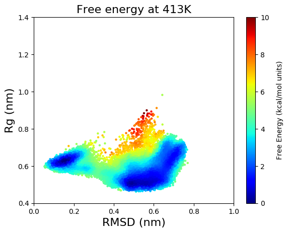
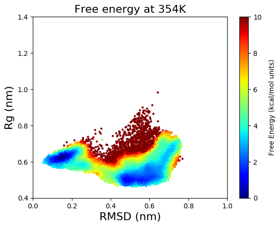
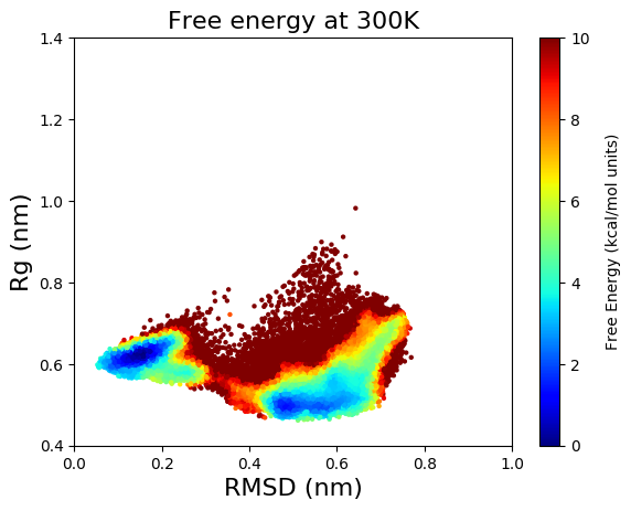
Figure 9: Free-energy obtained from an ISST trajectory for the in vacuum Alanine-12. The simulation started from the helical configuration and ran for $2.2\mu s$ using a 2 f$s$ timestep. The Amber96 force- field was used with a 20Å cut-off for electrostatics, constraining all bonds using the SNIP method.

We used GROMACS to extract the trajectory of the root mean square deviation (RMSD) and radius of gyration $R_{g}$ from the initial state. In Figure 9 we plot the free energy of the RMSD and $R_{g}$ at four temperatures. At the high temperature (top left panel) we observe 3 distinct states separated by energetic barriers. As the temperature decreases towards (from top left to bottom right) the free energy landscape changes into two distinct states separated by a large energetic barrier. As observed in [46], initializing a vanilla MD simulation in either basin at 300K will result in a skewed free energy landscape with no transitions between these two states.

In contrast, by using the ISST method we obtain improved sampling at all temperatures in the 300–500K range, both on the barriers and in the basins. We resolve, in detail, both the shape and the configurational states close to the states with minimal energy, giving a good overview of the structure of the free energy landscape and the available configurations at each temperature. Note that another benefit of ISST is that it significantly reduces the noise in the sampling compared to ST (this is clear from Sec. 4.2.3); ISST hence requires shorter trajectories and therefore less computational cost to achieve satisfactory results.

5 Concluding remarks

The theoretical analysis of the simulated tempering method that we performed in this paper allowed us to give it a firm theoretical justification and to draw several interesting connections between this and other sampling techniques. First we showed, as a consequence of a large deviation argument, that the optimal adjustment of temperature is via infinitely frequent switches, in which case it is possible to interpret the ST dynamics as being derived from a dynamical model for the positions and momenta alone using a modified potential energy function obtained by averaging. The equations of motions used in that model are the ones used in the integrate-over-temperature method of Gao [31]. Second we showed that it is preferable to think of the temperature as varying continuously in a range, in which case ST becomes a variant of the continuous tempering method proposed in Ref. [32]. Thirdly, we justified using the inverse of the partition function as temperature weights because of its flattening effect on the probability distribution of the system’s energy, which makes ISST the effective dual of the Wang-Landau method [5] in this case.

These theoretical considerations also permitted us to revisit in some detail the implementation of the ST method within a molecular dynamics framework. In particular we showed how to learn the partition function, and thereby the optimal temperature weights, in a simple adaptive way using a new estimator for this partition function. In our experiments on test models (harmonic oscillators, Curie-Weiss with second order phase transition; Alanine-12 molecule in vacuum), we found that the implementation of the ISST method was effective at accelerating sampling in challenging situations.

References

- [1] Daan Frenkel and Berend Smit. Understanding molecular simulation: from algorithms to applications, volume 1. Elsevier, 2001.
- [2] David J. C. MacKay. Information theory, inference, and learning algorithms. IEEE Transactions on Information Theory, 50:2544–2545, 2003.
- [3] Jean-Francois Richard and Wei Zhang. Efficient high-dimensional importance sampling. Journal of Econometrics, 141(2):1385–1411, 2007.
- [4] David P Landau and Kurt Binder. A guide to Monte Carlo simulations in statistical physics. Cambridge university press, 2014.
- [5] F. Wang and D. P. Landau. Efficient, multiple-range random walk algorithm to calculate the density of states. Phys. Rev. Lett., 86(10):2050–2053, 2001.
- [6] C. Junghans, D. Perez, and T. Vogel. Molecular dynamics in the multicanonical ensemble: Equivalence of wang–landau sampling, statistical temperature molecular dynamics, and metadynamics. Journal of Chemical Theory and Computation, 10:1843–1847, 2014.
- [7] A. Laio and M. Parrinello. Escaping free-energy minima. Proc. Nat. Acad. Sci., 99(20):12562–12566, 2002.
- [8] A. Barducci, G. Bussi, and M. Parrinello. Well-tempered metadynamics: A smoothly converging and tunable free-energy method. Phys. Rev. Lett., 100(2), 2008.
- [9] Luca Maragliano and Eric Vanden-Eijnden. A temperature accelerated method for sampling free energy and determining reaction pathways in rare events simulations. Chem. Phys. Lett., 426:168–175, 2006.
- [10] Cameron F Abrams and Eric Vanden-Eijnden. Large-scale conformational sampling of proteins using temperature-accelerated molecular dynamics. Proc. Nat. Acad. Sci. USA, 107(11):4961–4966, 2010.
- [11] E. Darve, D. Rodriguez-Gomez, and A. Pohorille. Adaptive biasing force method for scalar and vector free energy calculations. J. Chem. Phys., 128(14), 2008.
- [12] F. Aluffi-Pentini, V. Parisi, and F. Zirilli. Global optimization and stochastic differential equations. Journal of Optimization Theory and Applications, 47(1):1–16, 1985.
- [13] Rh Swendsen and Js Wang. Replica Monte Carlo simulation of spin glasses. Phys. Rev. Lett., 57(21):2607–2609, 1986.
- [14] Charles J Geyer. Markov Chain Monte Carlo Maximum Likelihood. Computing Science and Statistics: Proceedings of the 23rd Symposium on the Interface, (1):156–163, 1991.
- [15] Radford M. Neal. Sampling from multimodal distributions using tempered transitions. Statistics and Computing, 6(4):353–366, 1996.
- [16] Ulrich H.E. Hansmann. Parallel tempering algorithm for conformational studies of biological molecules. Chemical Physics Letters, 281(1-3):140–150, 1997.
- [17] Yuji Sugita and Yuko Okamoto. Replica-exchange molecular dynamics method for protein folding. Chemical Physics Letters, 314(1-2):141–151, 1999.
- [18] E Marinari, G Parisi, Dipartimento Fisica, Universitd Roma, Tor Vergata, and Sexione Roma Tor Vergatau -Rmna. Simulated Tempering: A New Monte Carlo Scheme. Europhys. Lett. Europhys. Lett, 19(196):451–458, 1992.
- [19] Ulrich H E Hansmann and Yuko Okamoto. Numerical Comparisons of Three Recently Proposed Algorithms in the Protein Folding Problem. J Comput Chem, 18:920–933, 1997.
- [20] Shinichi Banba, Zhuyan Guo, and Charles L Brooks III. Efficient sampling of ligand orientations and conformations in free energy calculations using the lambda-dynamics method. Journal Of Physical Chemistry B, 104(29):6903–6910, 2000.
- [21] Christopher J Woods, Jonathan W Essex, and Michael A King. Enhanced Configurational Sampling in Binding Free-Energy Calculations. Society, pages 13711–13718, 2003.
- [22] Ryan Bitetti-Putzer, Wei Yang, and Martin Karplus. Generalized ensembles serve to improve the convergence of free energy simulations. Chemical Physics Letters, 377(5-6):633–641, 2003.
- [23] Yuko Okamoto. Generalized-ensemble algorithms: Enhanced sampling techniques for Monte Carlo and molecular dynamics simulations. Journal of Molecular Graphics and Modelling, 22(5):425–439, 2004.
- [24] José D. Faraldo-Gómez and Benoît Roux. Characterization of Conformational Equilibria Through Hamiltonian and Temperature Replica-Exchange Simulations: Assessing Entropic and Environmental Effects. Journal of computational chemistry, 28:1634–1647, 2007.
- [25] Jozef Hritz and Chris Oostenbrink. Hamiltonian replica exchange molecular dynamics using soft-core interactions. Journal of Chemical Physics, 128(14), 2008.
- [26] Kei-ichi Okazaki, Nobuyasu Koga, Shoji Takada, Jose N Onuchic, and Peter G Wolynes. Multiple-basin energy landscapes for large-amplitude conformational motions of proteins: Structure-based molecular dynamics simulations. Proceedings of the National Academy of Sciences of the United States of America, 103(32):11844–9, 2006.
- [27] Yinglong Miao, William Sinko, Levi Pierce, Denis Bucher, Ross C Walker, and J Andrew Mccammon. Improved Reweighting of Accelerated Molecular Dynamics Simulations for Free Energy Calculation - Journal of Chemical Theory and Computation (ACS Publications). Journal of Chemical Theory and Computation, 10:2677–2689, 2014.
- [28] Pu Liu, Byungchan Kim, Richard a Friesner, and B J Berne. Replica exchange with solute tempering: a method for sampling biological systems in explicit water. Proceedings of the National Academy of Sciences of the United States of America, 102(39):13749–13754, 2005.
- [29] Nuria Plattner, J D Doll, Paul Dupuis, Hui Wang, Yufei Liu, and J E Gubernatis. An infinite swapping approach to the rare-event sampling problem. The Journal of chemical physics, 135(13):134111, oct 2011.
- [30] Paul Dupuis, Yufei Liu, Nuria Plattner, and J. D. Doll. On the Infinite Swapping Limit for Parallel Tempering. Multiscale Modeling & Simulation, 10(3):986–1022, 2012.
- [31] Yi Qin Gao. An integrate-over-temperature approach for enhanced sampling. Journal of Chemical Physics, 128(6), 2008.
- [32] Gianpaolo Gobbo and Benedict J. Leimkuhler. Extended hamiltonian approach to continuous tempering. Phys. Rev. E, 91:061301, Jun 2015.
- [33] Sanghyun Park and Vijay S Pande. Choosing weights for simulated tempering. Phys. Rev. E, 76(1):306, July 2007.
- [34] Gareth O Roberts and Jeffrey S Rosenthal. Minimising MCMC variance via diffusion limits, with an application to simulated tempering. Ann Appl Probab, 24(1):131–149, February 2014.
- [35] Zhiqiang Tan. Optimally adjusted mixture sampling and locally weighted histogram analysis. J. Comp. Graph. Stat., 26(1):54–65, 2017.
- [36] Yi Isaac Yang, Haiyang Niu, and Michele Parrinello. Combining Metadynamics and Integrated Tempering Sampling. arXiv.org, July 2018.
- [37] D. E. Carlson, P. Stinson, A. Pakman, and L. Paninski. Partition functions from Rao-Blackwellized tempered sampling. In Proceedings of the International Conference on Machine Learning, volume 48. JMLR W&CP, 2016.
- [38] Neal Madras and Mauro Piccioni. Importance sampling for families of distributions. Annals of Applied Probability, 9(4):1202–1225, January 1999.
- [39] M. D. Donsker and S.R.S. Varadhan. Asymptotic evaluation of certain Markov process expectations for large time, I. Comm. Pure Appl. Math., 28:1–47, 1975.
- [40] J. D. Deuschel and D. W. Stroock. Large deviation. Pure and Applied Mathematics, Vol. 137. Academic Press, New York, 1989.
- [41] Liming Wu. Large and moderate deviations and exponential convergence for stochastic damping Hamiltonian systems. Stoch. Proc. Appl., 91:205–238, 2001.
- [42] T. Bodineau and R. Lefevere. Large deviation of lattice Hamiltonian dynamics coupled to stochastic thermostats. J. Stat. Phys., 133:1–27, 2008.
- [43] Ben Leimkuhler and Charles Matthews. Molecular Dynamics With Deterministic and Stochastic Numerical Methods. Springer International Publishing, 1 edition, 2015.
- [44] Benedict Leimkuhler and Charles Matthews. Rational Construction of Stochastic Numerical Methods for Molecular Sampling. Applied Mathematics Research eXpress, 2013(1):34–56, 2013.
- [45] Phuong H Nguyen, Yuko Okamoto, and Philippe Derreumaux. Communication: Simulated tempering with fast on-the-fly weight determination. J Chem Phys, 138(6):061102, February 2013.
- [46] Iain Bethune, Ralf Banisch, Elena Breitmoser, Antonia B K Collis, Gordon Gibb, Gianpaolo Gobbo, Charles Matthews, Graeme J Ackland, and Benedict J Leimkuhler. MIST: A Simple and Efficient Molecular Dynamics Abstraction Library for Integrator Development. arXiv, May 2018.