PSR J2234$+$0611: A new laboratory for stellar evolution

Abstract

We report the timing results for PSR J2234$+$0611, a 3.6-ms pulsar in a 32-day, eccentric ($e\,=\,0.13$) orbit with a helium white dwarf. The precise timing and eccentric nature of the orbit allow measurements of an unusual number of parameters: a) a precise proper motion of 27.10(3) $\mathrm{mas\;yr^{-1}}$ and a parallax of 1.05(4) mas resulting in a pulsar distance of 0.95(4) kpc; enabling an estimate of the transverse velocity, 123(5) $\mathrm{km\;s^{-1}}$. Together with previously published spectroscopic measurements of the systemic radial velocity, this allows a 3-D determination of the system’s velocity; b) precise measurements of the rate of advance of periastron yields a total system mass of $1.6518^{+0.0033}_{-0.0035}$ M_⊙; c) a Shapiro delay measurement, $h_{3}\,=\,82\pm 14$ ns despite the orbital inclination not being near 90^∘; combined with the measurement of the total mass yields a pulsar mass of $1.353^{+0.014}_{-0.017}\,\mathrm{M_{\odot}}$ and a companion mass of $0.298^{+0.015}_{-0.012}\mathrm{M_{\odot}}$; d) we measure precisely the secular variation of the projected semi-major axis and detect significant annual orbital parallax; together these allow a determination of the 3-D orbital geometry of the system, including an unambiguous orbital inclination ($i\,=\,138.7^{+2.5}_{-2.2}\deg$) and a position angle for the line of nodes ($\Omega\,=\,44^{+5}_{-4}\deg$). We discuss the component masses to investigate the hypotheses previously advanced to explain the origin of eccentric MSPs. The unprecedented determination of the 3-D position, motion and orbital orientation of the system, plus the precise pulsar and WD masses and the latter’s optical detection make this system an unique test of our understanding of white dwarfs and their atmospheres.

1 Introduction

Millisecond pulsars (MSPs) are a population of pulsars with much faster spin rates and significantly smaller spin-down rates than that of the “normal” pulsars. They are believed to be formed through a process in which a neutron star (NS) goes through a long period of accretion from a companion star. This mass transfer process circularizes the orbit and results in the neutron star spinning faster and a reduction in the neutron star’s magnetic field. If the companion is a low-mass star, then the system is seen during accretion as a low-mass X-ray binary (LMXB; Alpar et al., 1982; Radhakrishnan & Srinivasan, 1982). The tidal circularization for these systems results invariably in orbits with very low eccentricities. The result of the evolution of a LMXB is a MSP orbited by a helium white dwarf (He WD). A fundamental expectation of this process is that the orbit of a MSP - He WD should have a very low eccentricity (Phinney, 1992), since the formation of the companion He WD is not associated with violent events, like supernova explosions. This is confirmed by the very small eccentricities measured for the vast majority of MSPs with He WD companions.

In recent years, a small set of systems that are inconsistent with the typical formation scenario have been discovered in the Galactic field: PSRs J0955$-$6150 (Camilo et al., 2015), J1618$-$3921 (Edwards & Bailes, 2001; Octau et al., 2018), J1946$+$3417 (Barr et al., 2013), J1950$+$2414 (Knispel et al., 2015) and J2234$+$0611 (Deneva et al., 2013); the latter will be the focus of this work. All have orbital eccentricities in the range 0.027 - 0.14 and small mass ($\sim\,0.3\,M_{\odot}$) companions. Additionally, the orbital periods for these systems are quite similar ($P_{b}\sim 22\,-\,32$ d, see Figure 1).

The first known MSP with an eccentric orbit in the Galactic field, PSR J1903+0327 (Champion et al., 2008) (with an orbital period of 95 d and orbital eccentricity of 0.43, the companion is a 1.03 $\mathrm{M_{\odot}}$ main sequence star), is thought to have formed in the chaotic disruption of a triple system (Freire et al., 2011). This is not a likely explanation for the former systems given the similarity of their orbital parameters. A number of hypotheses for their formation have been advanced, including rotationally delayed accretion induced collapse (Freire & Tauris, 2014), a phase transition inside the MSP that results in the formation of a strange star core (Jiang et al., 2015) and eccentricity pumping via interaction with a circumbinary disk (Antoniadis et al., 2016a).

In wide, circular MSP systems, the only relativistic parameters that can be measured are the ‘range’ ($r$) and ‘shape’ ($s$) parameters of a Shapiro delay. Such measurements are only possible for systems with high orbital inclinations and where the pulsar has high timing precision, or the companion is massive. The result is that only four systems have NS mass measurements better than 5% from Shapiro delay alone (PSR J2222$-$0137, Cognard et al. 2017, PSRs J1909$-$3744, J1614$-$2230 and J1713$+$0747, Arzoumanian et al. 2018). If the wide MSP binary is eccentric, then we can also measure the advance of periastron ($\dot{\omega}$), which gives a measurement of the total system mass ($M_{\rm tot}$). This, together with even a poorly determined Shapiro delay, allows the measurement of precise MSP masses (Freire et al., 2011; Lynch et al., 2012; Barr et al., 2017), but this is a relatively rare occurrence since eccentric MSP systems are rare. Using this technique, the masses of two of the eccentric MSPs, PSRs J1946+3417 and J1950+2414, have already been measured precisely by Barr et al. (2017) and Zhu et al. (in preparation); the pulsar masses are $1.828(22)\,\rm M_{\odot}$ and $1.495(24)\,M_{\odot}$ respectively and the companion masses are $0.2556(19)\,\rm M_{\odot}$ and $0.280_{-0.004}^{+0.006}\,M_{\odot}$ respectively.

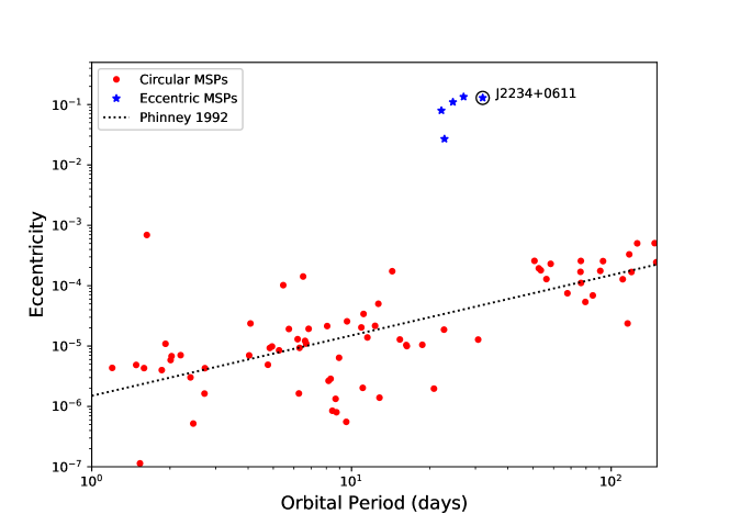
Figure 1: Eccentricity ($e$) versus orbital period ($P_{\rm b}$) for recycled pulsars with low-mass ($<0.6\,\mathrm{M_{\odot}}$) companions outside globular clusters. The eccentric MSPs, blue stars, stand out from the general MSP population, red circles. For the latter, the orbital eccentricities are small and generally follow the evolution predicted by Phinney (1992), shown by the black dotted line. Note that there is an under-density of circular MSP systems within the orbital period range where the eccentric MSPs are found and going to larger orbital periods, as first noted by (Camilo, 1995).

In this paper, we present a study of PSR J2234+0611, an eccentric MSP system for which the precise timing has, as in the case of PSR J1946+3417 and J1950+2414, enabled precise mass measurements for both the pulsar and its companion. In Section 2, we detail the detection and follow-up timing observations. In Section 3, we describe the phenomenological development of the timing model, enumerating the different orbital effects that are detectable in this system and present some initial results. In Section 4, we extend on the preliminary results using Bayesian methods to determine the masses and orbital orientation of the system in a self-consistent way, assuming the validity of general relativity. In Section 5, we discuss the implications of our findings. In Section 6, we summarize our conclusions for this system.

Some of these results have already been presented preliminarily by Antoniadis et al. (2016a), who confirmed, based on the timing position of the system, that the companion is a He WD. From the spectroscopy of the WD, they placed limits on the systemic radial velocity of the system, $\mathrm{V_{r}\approx-20(34)\;km\;s^{-1}}$. They used this, together with our preliminary timing values for the proper motion and the distance, to study the system’s 3-D motion in the Galaxy.

2 Observations and Analysis

2.1 Discovery and observations

PSR J2234$+$0611 was discovered in the Arecibo Observatory 327 MHz Drift Scan Survey in December 2012 (Deneva et al., 2013). After discovery of the pulsar, initial follow-up observations were performed, also with the Arecibo 305-m telescope, using the “L-wide” receiver at a center frequency of 1.5 GHz and recorded with the Puerto Rican Ultimate Pulsar Processing Instrument (PUPPI) in search mode, allowing for offline folding of each observation to get the observed period at each epoch. The preliminary orbital parameters resulting from these observations were already reported in Deneva et al. (2013).

We then folded the data using the new orbit and began to refine the timing solution by generating pulse times-of-arrival (ToAs) and performing pulsar timing analysis using tempo. Subsequent data was recorded using PUPPI in coherent dedispersion and online folding mode. Figure 2 shows the profile for PSR J2234+0611 at 430 and 1.5 GHz from roughly 30-minute duration coherent fold mode observations.

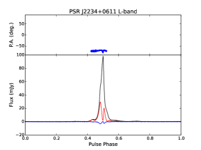
Figure 2: Polarimetric profiles for PSR J2234+0611 at 430 MHz (left) and 1.5 GHz (right) from the Arecibo Observatory using the PUPPI backend with bandwidths of 20 and 650 MHz, respectively. These profiles were taken from individual high signal-to-noise ratio detections. The top panels show the polarization angle versus pulse phase. The bottom panels show the total intensity (black), linear polarization (red), and circular polarization (blue) versus pulse phase. The profiles have been polarization and flux calibrated using the methods described in  Arzoumanian et al. (2018). These profiles have not been corrected for rotation measure, as the value measured from these observations is consistent with 0 $\mathrm{rad\;m^{-2}}$. Additional analysis of the polarization properties for PSR J2234$+$0611 has been presented in Gentile et al. (2018).

PSR J2234+0611 was immediately found to have excellent timing precision and therefore was added to the pulsar timing arrays (PTAs) efforts to detect low frequency gravitational waves, in particular to the North American Nanohertz Observatory for Gravitational Waves (NANOGrav, Demorest et al., 2013) PTA. Observations of the pulsar have continued under that project, using the Arecibo 305-m radio telescope with the “L-wide” receiver (with frequency coverage between 1130 and 1730 MHz) and the 430 MHz receiver with a cadence of about 3 weeks. For both types of observations, the PUPPI back-end was used, with coherent dedispersion and folding mode, as for other PTA pulsars; these observations are described in detail by Arzoumanian et al. (2018) but extend later in time than the data presented in that paper. Current timing solution parameters from data spanning 5 years are given in Tables 1 and 2.

Figure 3: Five years of high-precision timing data for PSR J2234+0611. Top: Dispersion measure offsets relative to the reference DM (10.778 cm${}^{-3}\,$pc) as a function of date. Middle: ToA residuals for the DDGR ephemeris in Table 1 as a function of date, and Bottom: ToA residuals as a function of the orbital phase. The residual 1-$\sigma$ uncertainties are indicated by vertical error bars. Black indicates the data from the initial incoherent observations at 1.5 GHz, blue data from the coherent observations at 1.5 GHz and red the coherent observations at 430 MHz. There is a jump in the measured DM offsets between the incoherent observations and the coherent observations due to covariances between the DM offsets and a constant offset between the two datasets.

2.2 Timing analysis

The timing analysis of the PUPPI data is similar to that described by Arzoumanian et al. (2018). The ToAs are derived from the integrated pulse profiles using the standard PSRCHIVE routines. The ToA analysis is made using tempo. To convert the telescope ToAs (corrected to the International Bureau of Weights and Measures version of Terrestrial Time, TT) to the Solar System barycentre, we used the Jet Propulsion Laboratory’s DE436 solar system ephemeris; the resulting timing parameters are presented in Barycentric Dynamical Time (TDB). We used the same method used by NANOGrav to estimate variations of the dispersion measure (DM), but with the ToAs grouped in intervals of 32 days (the orbital period), instead of 6 days as is the norm for the NANOGrav pulsars. DM values are reported as offsets relative to an arbitrary fiducial value of 10.778 pc cm^-3.

We used three orbital models to analyze the data, all based on the description of Damour & Deruelle (1985, 1986). The first is the “DDGR” model, which assumes the validity of general relativity (GR) and where we fit directly for the total mass of the system ($M_{\rm tot}$) and the companion mass ($M_{c}$). The second model is basically the theory-independent DD model, but with the orthometric parameterization of the Shapiro delay described by Freire & Wex (2010); this was implemented in tempo by Weisberg & Huang (2016), where it is designated as the “DDFWHE" orbital model. The third model is again based on the DD model but takes into account the kinematic effects described by Kopeikin (1995, 1996); this was implemented in tempo2 by Edwards et al. (2006), where it is designated as the “T2” model; it was implemented in tempo by one of us (IHS), where it is designated as the “DDK” model.

The reason for the usage of these three orbital models is that, as we will show, no single model alone fully captures all the constraints on the masses and orbital orientation of this system. In the DDFWHE and DDK solutions, we used the Einstein delay calculated in the DDGR solution; the reason for this is because it cannot be determined independently with our data, and because it is strongly correlated with $\dot{x}$ (see Ridolfi et al. 2018, in preparation). Furthermore, the orthometric ratio of the Shapiro delay ($\varsigma$) in the DDFWHE solution and the orbital inclination ($i$) in the DDK solution are derived from the $s\,\equiv\,\sin i$ parameter calculated by the DDGR solution; the reason being the extremely small signature of the Shapiro delay. In Section 3, we discuss the significance of these parameters.

2.3 Flux Measurements

As part of the NANOGrav data analysis procedures, the data have been flux and polarization calibrated, allowing straightforward measurements of the polarization profile (Figure 2) and mean flux density. We have taken flux density values from a preliminary analysis of the upcoming 12.5 year data release (Arzoumanian et al., in prep.). The data in this preliminary release was polarization and flux calibrated using the same methods as the NANOGrav 9-year data release (The NANOGrav Collaboration et al., 2015). However, the observed flux density for PSR J2234$+$0611 varies over a fairly wide range due to scintillation by the interstellar medium. Using psrflux from the PSRCHIVE pulsar suite, we calculated the mean value from 43 observations at 430 MHz, ranging from 0.2 to 5.3 mJy and 50 observations at 1.5 GHz, ranging from 0.03 to 3.3 mJy to get an estimate for the mean flux density at these frequencies. The resulting mean values and spectral index are given in Table 1.

Table 1: Non-binary parameters for PSR J2234+0611

Observation and data reduction parameters
Reference Epoch (MJD)	56794.093186
Span of timing data (MJD)	56347 - 58291
Number of ToAs	5882
Solar wind parameter, $n_{0}$ (cm-3)	6
Overall individual ToA RMS residual ($\mu s$)	0.58
RMS residual for incoherent L-band ($\mu s$)	0.35
RMS residual for coherent 430 MHz ($\mu s$)	1.51
RMS residual for coherent L-band ($\mu s$)	0.59
$\chi^{2}$	5891.76
Reduced $\chi^{2}$	1.013
Spectral parameters
Mean flux density at 430 MHz, $S_{430}$ (mJy)	1.3
Mean flux density at 1400 MHz, $S_{1400}$ (mJy)	0.6
Spectral Index, $\alpha$	$-0.7$
Astrometric and spin parameters
Right ascension, $\alpha$ (J2000)	22:34:23.073090(2)
Declination, $\delta$ (J2000)	06:11:28.68633(7)
Proper motion in $\alpha$, $\mu_{\alpha}$ ($\mathrm{mas\;yr^{-1}}$)	25.30(2)
Proper motion in $\delta$, $\mu_{\delta}$ ($\mathrm{mas\;yr^{-1}}$)	9.71(5)
Parallax, $\varpi$ (mas)	1.03(4)
Spin frequency, $\nu$ (Hz)	279.5965821510426(5)
Spin frequency derivative, $\dot{\nu}$ ($10^{-16}\,\rm Hz\,s^{-1}$)	$-$9.3920(1)
Dispersion measure, DM ($\rm pc\,cm^{-3}$)	10.778
Derived parameters
Galactic longitude, $l$	+72.99
Galactic latitude, $b$	$-$43.01
Magnitude of proper motion, $\mu$ ($\rm mas\,yr^{-1}$)	27.10(2)
Position angle of proper motion, $\Theta_{\mu}$ ($\deg$, J2000)	69.0(1)
Position angle of proper motion, $\Theta_{\mu}$ ($\deg$, Galactic)	111.5(1)
DM-derived distance, $d_{1}$ (kpc)	0.68
DM-derived distance, $d_{2}$ (kpc)	0.86
Parallax-derived distance, $d$ (kpc)	0.97(4)
Galactic height, $z$ (kpc)	-0.651(26)
Transverse velocity, $v_{\rm T}$ ($\rm km\,s^{-1}$)	123(5)
Spin period, $P$ (ms)	3.576581631673107(6)
Spin period derivative, $\dot{P}$ ($10^{-20}$ s s-1)	1.20142(1)
Intrinsic spin period derivative, $\dot{P}_{\rm int}$ ($10^{-20}$ s s-1)	$0.647^{+0.023}_{-0.025}$
Surface magnetic flux density, $B_{0}$ ($10^{8}$ Gauss)	1.5
Characteristic age, $\tau_{c}$ (Gyr)	8.8
Spin-down power, $\dot{E}$ ($10^{33}\,\rm erg\,s^{-1}$)	5.6
Notes. Timing parameters and 1-$\sigma$ uncertainties derived using tempo in
Barycentric Dynamical Time (TDB), using the DE 421 Solar System ephemeris,
the NIST UTC time timescale and the DDGR orbital model.
$d_{1}$ is derived using the NE2001 (Cordes & Lazio, 2002) Galactic model,
$d_{2}$ using the YMW16 (Yao et al., 2017) Galactic model.
Estimate of $v_{\rm T}$, $\dot{P}_{\rm int}$ and derived parameters assume distance from measured
parallax and its uncertainty.

Table 2: Orbital parameters for PSR J2234+0611

Orbital model	DDGR	DDFWHE	DDK	DDK Bayesian grid
Residual $\chi^{2}$	5891.8	5891.7	5872.9
Reduced $\chi^{2}$	1.013	1.013	1.010
Orbital period, $P_{\rm b}$ (days)	32.001401626(8)	32.001401627(8)	32.001401630(8)	-
Projected semi-major axis, $x$ (lt-s)	13.937366(5)	13.9373664(3)	13.9373664(3)	-
Epoch of periastron, $T_{0}$ (MJD)	56794.0931866(1)	56794.0931866(1)	56794.0931866(1)	-
Orbital eccentricity, $e$	0.129274035(5)	0.129274034(8)	0.129274035(8)	-
Longitude of periastron, $\omega$ (∘)	277.1673(2)	277.167331(1)	277.167330(1)	-
Total mass, $M_{\rm tot}$ ($\rm M_{\odot}$ )	1.679(3)	-	-	$1.6518^{+0.0033}_{-0.0035}$
Companion mass, $M_{c}$ ($\rm M_{\odot}$ )	0.300(13)	-	0.30(5)	$0.298^{+0.015}_{-0.012}$
Shapiro delay $s$	[0.667765]	-	-	-
Rate of advance of periastron, $\dot{\omega}$ ($\deg\,\rm yr^{-1}$)	[0.0008863]	0.0008863(10)	0.0008766(10)	-
Einstein delay, $\gamma$ (s)	[0.000847606]	[0.000847606]	[0.000847606]	-
Derivative of $P_{\rm b}$, $\dot{P}_{\rm b}$ ($10^{-12}$ s s-1)	1.8(2.5)a	1.9(2.5)	3.1(2.5)	-
Orthometric amplitude of Shapiro delay, $h_{3}$ (ns)	-	82(14)	-	-
Orthometric ratio of Shapiro delay, $\varsigma$	-	$0.382811^{\rm b}$	-	-
Derivative of $x$, $\dot{x}$ ($10^{-15}$ lt-s s-1)	$-$27.8(7)	$-$27.8(7)	-	-
Orbital inclination ($\deg$)	-	-	$138.105^{\rm b}$	$138.7^{+2.5}_{-2.2}$
Position angle of line of nodes, $\Omega$ ($\deg$)	-	-	43.4(7)	$44^{+5}_{-4}$
Derived parameters
Mass function, $f$ ($\rm M_{\odot}$ )	0.002838487(3)	0.0028384868(2)	0.0028384867(2)	-
Pulsar mass, $M_{p}$ ($\rm M_{\odot}$ )	1.38(1)	-	-	$1.353^{+0.014}_{-0.017}$
Notes. Timing parameters and 1-$\sigma$ uncertainties derived using tempo, in Barycentric Dynamical Time (TDB)
using JPL’s DE421 Solar System Ephemeris and the NIST UTC timescale.
Numbers in square brackets are derived by the DDGR model. Of these, $\gamma$ is used in the DDFWHE and DDK models.
a: Fitted as an extra contribution to the (very small) relativistic $\dot{P}_{\rm b}$ in the DDGR solution.
b: Assumed in the model, derived from $s$ parameter in the DDGR solution.

Table 3: Details for grid regions.

Region	$\cos{i}$	$\Omega$	Best $\cos(i)$	Best $\Omega$	Best $\rm M_{tot}$	Min $\chi^{2}$
1	$-$0.92 to -0.52	34∘ to 54∘	-0.748	43.8	1.6512	5872.9
2	0.52 to 0.92	90.0∘ to 110.0∘	0.748	94.4	1.6518	5881.7
3	0.52 to 0.92	210.0∘ to 230.0∘	0.716	220.6	1.7058	5926.0
4	$-$0.92 to -0.52	270.0∘ to 290.0∘	-0.704	278.4	1.7058	5929.6

3 Results

The timing parameters resulting from the timing models described before are given in Tables 1 and 2. The spin and astrometric parameters derived from the DDGR orbital solution are presented in Table 1; the reason for only presenting this solution is that these parameters are nearly identical for the other orbital solutions. The orbital parameters for the three solutions are presented in Table 2, as well as the results from the Bayesian analysis described in Section 4, which yields the most reliable parameters and uncertainties. We have applied EFACs, a multiplication factor for the ToA uncertainties, and EQUADs, an error term added in quadrature to the ToA uncertainties, for each receiver and backend configuration, and have also allowed a fit for an arbitrary offset between the 3 types of data; 1.5 GHz incoherent, 430 MHz coherent, and the 1.5 GHz coherent. For the 5882 ToAs used in our analysis, we obtain a weighted residual root mean square (rms) of 0.58 $\mu$s and a reduced $\chi^{2}$ of 1.013 for the best orbital model (DDK). The evolution of the DM with time and the ToA residuals with time are displayed in Fig. 3; the residuals are also presented as a function of the orbital phase.

3.1 Distance and velocity

For this pulsar, we obtain a highly significant measurement of the parallax, 1.05(4) mas (all uncertainties are 68.3% confidence limits) resulting in a pulsar distance $d$ of 0.95(4) kpc. This distance can be compared with the prediction of the DM models. The NE2001 model (Cordes & Lazio, 2002) predicts a distance of 0.68 kpc, while the YMW16 model (Yao et al., 2017) predicts a distance of 0.86 kpc. To these estimates is generally assigned a relative uncertainty of about 20%. Our parallax measurement is certainly in better agreement with the YMW16 model.

This measurement, together with the measurement of the proper motion, allows a relatively accurate measurement of the Heliocentric transverse velocity, 123(5) $\mathrm{km\;s^{-1}}$. Combining this with the systemic radial velocity of $-20(34)\,\rm km\,s^{-1}$ measured by Antoniadis et al. (2016a), we obtain a 3-D heliocentric velocity of $124^{+10}_{-5}\mathrm{km\;s^{-1}}$. This velocity is smaller than that used in the detailed analysis of the Galactic motion of PSR J2234+0611 made by Antoniadis et al. (2016a), mostly because they were using a preliminary value of the parallax that yielded a larger distance, however the qualitative conclusions obtained by Antoniadis et al. (2016a) remain valid: the 3-D velocity of this system is similar to what has been observed for other nearby recycled pulsars (e.g., Gonzalez et al. 2011). We will return to this topic in Section 5, particularly in the discussion on the formation of the system.

3.2 Kinematic effects: Rate of change of Doppler shift

For any assumed distance we can estimate the magnitude of the kinematic effects on the variation of the Doppler shift factor ($D$) using the simple expressions provided by Shklovskii (1970) for the effect of the centrifugal acceleration (proportional to the square of the total proper motion, $\mu$) and Damour & Taylor (1991) for the effect of the difference in the Galactic accelerations of the pulsar’s system and the Solar System projected along the direction from the pulsar to the Earth, $a_{l}$:

$$\frac{\dot{D}}{D}\,\equiv-\frac{\mu^{2}d+a_{l}}{c}$$ (1)

where $c$ is the speed of light. In order to estimate $a_{l}$, we use the expressions presented by Lazaridis et al. (2009), where the equation for the vertical acceleration should be valid to a Galactic height of $\sim\,\pm 1.5$ kpc (the Galactic height of PSR J2234+0611 is $-$0.651(26) kpc). In those expressions we use the distance to the centre of the Galaxy measured by the GRAVITY experiment (Gravity Collaboration et al., 2018), $r_{0}\,=\,8.122(31)$ kpc and a revised value for the rotational velocity of the Galaxy derived using the latter $r_{0}$ (McGaugh, 2018), $v_{\rm Gal}\,=\,233.3$ km s^-1. We obtain $a_{l}/c\,=\,-1.53\,\times\,10^{-19}\,\rm s^{-1}$ (for a comparison, we can use the Galactic model presented by McMillan (2017) to obtain $a_{l}/c\,=\,-1.76\,\times\,10^{-19}\,\rm s^{-1}$, which is a similar number). For the proper motion term we obtain $\mu^{2}d/c\,=\,1.702\,\times\,10^{-18}\,\rm s^{-1}$, an order of magnitude larger. Adding both terms, we obtain $\dot{D}/D\,=\,-1.550\,\times\,10^{-18}\,\rm s^{-1}$.

The contribution of this effect to the spin period derivative is given by $\dot{P}_{\rm kin}\,=\,-P\,\dot{D}/D\,=\,5.54_{-0.25}^{+0.23}\,\times\,10^{-21}\,\rm s\,s^{-1}$. Subtracting this from the observed $\dot{P}$ in Table 1 we obtain the intrinsic spin period derivative ($\dot{P}_{\rm int}\,=\,6.47_{-0.25}^{+0.23}\,\times\,10^{-21}\,\rm s\,s^{-1}$), which is about half of the observed $\dot{P}$. From this and the spin period $P$, we derive a surface magnetic flux density $B_{0}\,\simeq\,1.5\,\times\,10^{8}\,\rm G$, the rate of loss of rotational energy $\dot{E}\,\simeq\,5.6\,\times 10^{33}\,\rm erg\,s^{-1}$ and a characteristic age $\tau_{c}\,\simeq\,8.8\,\rm\,Gyr$ using the standard equations summarized by Lorimer & Kramer (2004). The cooling age for the WD companion is 1.5 Gyr, which according to Antoniadis et al. (2016a) is comparable to the age of the system. This is compatible with $\tau_{c}$ since the latter represents an upper limit for the age that assumes that the initial spin period $P_{\rm init}$ was much smaller than the currently observed $P$. Assuming a $n\,=\,3$ braking index and an age of 1.5 Gyr, we obtain $P_{\rm init}\,=\,3.25\,\rm ms$.

3.3 Post-Keplerian effects. I. Orbital period derivative

This rate of change of the Doppler shift factor will also be a dominant contributor to the observed variation of the orbital period, $\dot{P}_{\rm b,obs}$. According to Lorimer & Kramer (2004):

$$\left(\frac{\dot{P}_{\rm b}}{P_{\rm b}}\right)^{\rm obs}\,=\,-\,\frac{\dot{D}}{D}\,+\,\left(\frac{\dot{P}_{\rm b}}{P_{\rm b}}\right)^{\rm GW}\,+\,\left(\frac{\dot{P}_{\rm b}}{P_{\rm b}}\right)^{\rm\dot{m}}\,+\,\left(\frac{\dot{P}_{\rm b}}{P_{\rm b}}\right)^{\rm T},$$ (2)

the first term, the kinematic contribution to $\dot{P}_{\rm b,obs}$ is given by $\dot{P}_{\rm b,kin}\,=\,-P_{\rm b}\,\dot{D}/D\,=\,4.28^{+0.19}_{-0.18}\,\times\,10^{-12}\,\rm\,s^{-1}$. The second term in eq. 2 is due to loss of orbital energy caused by the emission of gravitational waves. For PSR J2234+0611, this term is, assuming the validity of GR, given by $\dot{P}_{\rm b,GR}\,=\,2.62\,\times\,10^{-17}\,\rm s\,s^{-1}$ (this is the estimate provided by the DDGR model for the masses derived by that model). This is about 5 orders of magnitude smaller than $\dot{P}_{\rm b,obs}$ and its uncertainty. The third term is caused by radiative mass loss from the system. Assuming that this is dominated by the loss of rotational energy for the pulsar, it is given by Damour & Taylor (1991):

$$\left(\frac{\dot{P}_{\rm b}}{P_{\rm b}}\right)^{\rm\dot{m}}\,=\,\frac{8\pi G}{T_{\odot}c^{5}}\frac{I}{M_{\rm tot}}\frac{\dot{P}_{\rm int}}{P^{3}}\,\sim\,3.8\,\times\,10^{-21}\rm s^{-1}$$ (3)

where $T_{\odot}=GM_{\odot}c^{-3}=4.925490947\mu\rm s$ is a solar mass ($M_{\odot}$) in time units, $c$ is the speed of light and $G$ is Newton’s gravitational constant, $I$ is the moment of inertia of the pulsar, $I\,\simeq\,10^{38}\rm\,kg\,m^{2}$. Thus $\dot{P}_{\rm b}^{\dot{m}}\,=\,1.05\,\times\,10^{-14}\,\rm s\,s^{-1}$, which is about 40 times smaller than $\dot{P}_{\rm b,kin}$. Finally, the last term in eq. 2 is caused by tidal dissipation. For PSR J2234+0611, this term should be negligible: the WD mass and atmospheric parameters, indicate that the star is well within its Roche lobe and no mass loss occurs. Consequently, the tidal dissipation timescale (Zahn, 1977) is of order 20 Gyr, well above the characteristic age of the pulsar; $\tau_{\rm c}\simeq 1.5$ Gyr.

Thus the only relevant term appears to be $\dot{P}_{\rm b,kin}$. This matches the observation ($\dot{P}_{\rm obs}\,=\,3.3\,\pm\,2.5\,\times\,10^{-12}\,\rm s\,s^{-1}$ for the DDGR and DDFWHE solutions, $\dot{P}_{\rm obs}\,=\,4.9\,\pm\,2.5\,\times\,10^{-12}\,\rm s\,s^{-1}$ for the DDK solution, see Table 2) well; for the DDK solution we have a 2-$\sigma$ “detection” of this effect.

Figure 4: Mass constraints for PSR J2234+0611. In the main plot on the left we display the $\cos i$ - $M_{c}$ plane; the gray region is excluded by knowledge of the mass function and the fact that the pulsar mass ($M_{p}$) must be larger than 0. In the main plot on the right, we display the $M_{p}$-$M_{c}$ plane; the gray region is excluded by knowledge of the mass function and the constraint $\sin i\,\leq\,1$. In both plots, the yellow region is excluded by the measurement of $\dot{x}$. The black contours include 68.23 and 95.44% of the total probability density functions (pdf) derived from a 3-D quality ($\chi^{2}$) map of the $\cos i$-$\Omega$-$M_{\rm tot}$ plane using the DDK orbital model, with the additional assumption that GR is the correct theory of gravity, see text for details. The solid blue lines indicate the regions that are (according to GR) consistent with the nominal and $\pm\,1-\sigma$ measurements of $h_{3}$ (solid) in the DDFWHE model, the blue dashed lines indicate the assumed $\varsigma$ (dashed) in that model (see Table 2). The solid red lines indicate the 0, $\pm\,1$-$\sigma$ constraints derived from the $\dot{\omega}_{\rm obs}$ in the DDFWHE model, these are equivalent to the $M_{\rm tot}$ in the DDGR model. The dashed red lines indicate the minimal and maximal values of $M_{\rm tot}$ taking into account the full range of possible contributions of the proper motion to $\dot{\omega}_{\rm obs}$, this is $\dot{\omega}_{\rm k}\,=\,\pm\,\mu/\sin i$

(see text for details). The side panels display the 1-d pdfs for $\cos i$ (top left), $M_{p}$ (top right) and $M_{c}$ (right). The vertical lines in these pdfs indicate the median and the percentiles corresponding to 1 and 2 $\sigma$ around the median.

3.4 Post-Keplerian effects. II. Secular rate of advance of periastron

The post-Keplerian effect measured to highest significance for PSR J2234+0611 is the rate of advance of periastron, $\dot{\omega}$. According to Lorimer & Kramer (2004), the observed effect is given, in the absence of a third component in the system, by:

$$\dot{\omega}_{\rm obs}\,=\,\dot{\omega}_{\rm rel}+\dot{\omega}_{\rm k}+\dot{\omega}_{\rm SO}$$ (4)

The third term is caused by spin-orbit coupling, a result of the finite size of the companion white dwarf, for wide systems like PSR J2234+0611 this effect is negligible.

The first term is caused by relativistic effects. Assuming GR, we can estimate the total mass of the binary, $M_{\rm tot}$ (Robertson, 1938) from $\dot{\omega}_{\rm rel}$ by inverting the well-known expression derived by Taylor & Weisberg (1982):

$$M_{\rm tot}\,=\,\frac{1}{T_{\odot}}\left[\frac{\dot{\omega}_{\rm Rel}}{3}(1-e^{2})\right]^{\frac{3}{2}}\left(\frac{P_{\mathrm{b}}}{2\pi}\right)^{\frac{5}{2}}.$$ (5)

The DDGR model assumes that $\dot{\omega}_{\rm rel}\,=\,\dot{\omega}_{\rm obs}$, i.e., all other terms are assumed to be negligible. As we see below this assumption cannot be made for PSR J2234+0611. From this assumption, the DDGR model obtains $M_{\rm tot}\,=\,1.6798(29)\,\rm M_{\odot}$. The $\dot{\omega}$ provided by the DDFWHE solution yields, assuming GR, an identical $M_{\rm tot}$. This constraint is represented by the solid red line in Figure 4.

However, the $\dot{\omega}$ measured by the DDK solution is smaller than that measured by the DDFWHE model by a small ($\Delta\dot{\omega}\,=\,9.60\,\times\,10^{-6}\,\deg\,\rm yr^{-1}$) but highly significant (9.3  $\sigma$) amount. The reason is that, for PSR J2234+0611, as for another wide, precisely timed system, PSR J1903+0327 (Freire et al., 2011) the second term in eq. 4, $\dot{\omega}_{\rm k}$, is larger than the measurement uncertainty. This term is given by Kopeikin (1995), here re-arranged as in Freire et al. (2011):

$$\dot{\omega}_{\rm k}\,=\,\frac{\mu}{\sin i}\cos\left(\Theta_{\mu}-\Omega\right),$$ (6)

where $\Theta_{\mu}$ is the position angle (PA) of the proper motion and $\Omega$ is the PA for the line of nodes. In the DDK orbital model, the PAs are measured in Equatorial (J2000) coordinates, starting from North through East and an inclination smaller than $90^{\circ}$ corresponds to a system where the line-of-sight component of the angular momentum points towards the Earth.

Although $\Theta_{\mu}$ is measured directly from the proper motion (see Table 1), the orientation of the line of nodes $\Omega$ is generally harder to determine. In fig. 4, we display with the dashed red lines the total masses assuming minimal or maximal contributions of $\dot{\omega}_{\rm k}$ to $\dot{\omega}_{\rm obs}$, $M$ (estimated from equation 6 by setting $\cos\left(\Theta_{\mu}-\Omega\right)\,=\,\pm\,1$). This shows clearly that $\dot{\omega}_{\rm k}$ is potentially much larger than the uncertainty in the measurement of $\dot{\omega}_{\rm obs}$.

However, we can estimate the total mass more accurately since, in the DDK model, we can determine $i$ and $\Omega$ with high precision (see details in section 3.6, and DDK solution in Table 2). Using these values the model internally estimates $\dot{\omega}_{\rm k}$ and automatically subtracts it from the “measured” $\dot{\omega}_{\rm obs}$, reporting only the part (presumably) caused by the relativistic effects, $\dot{\omega}_{\rm rel}$. Assuming GR, this yields a lower binary mass ($M_{\rm tot}\,=\,1.6526(29)\,\rm M_{\odot}$) than estimated by the DDGR model. We consider this to be accurate since it takes the proper motion into account.

3.5 Post-Keplerian effects. III. Shapiro delay

In the DDGR model, we not only obtain a precise (but in this case innacurate) estimate for $M_{\rm tot}$, but also a precise estimate for the companion mass ($M_{c}\,=\,0.300(13)\,\rm M_{\odot}$). Given the mass function of the system, the estimated $M_{c}$ implies $\sin i\,\sim\,0.668$; this implies either $i\,\sim 42\deg$ or $i\,\sim 138\deg$. The measurement is possible because of the presence of the Shapiro delay, however, the fact that the Shapiro delay is detected at all for a system with an orbital inclination so far from edge-on (90^∘) is unusual. The detection in this case is the is result of two factors: one is the high timing precision of the Arecibo observations of this pulsar, the second is the large eccentricity of the orbit; the latter helps separate the Shapiro delay from the normal “Roemer” delays caused by the geometry of the orbital motion relative to the line of sight.

The far from edge-on inclination means that the Shapiro delay is not easy to measure. When using the DDFWHE model to fit for both Shapiro delay parameters, $h_{3}$ and $\varsigma$, both values are measured to relatively low confidence. In order to better quantify the Shapiro delay, we use the best-fit value of $s\equiv\sin i$ that corresponds to the masses determined by the DDGR model ($s\,=\,0.6677654...$) to derive (Freire & Wex, 2010):

$$\varsigma\,=\,\frac{s}{1+\sqrt{1-s^{2}}}=0.382811...,$$ (7)

this is represented by the blue dashed line in figures 4 and 5. Fixing this in the DDFWHE model, we obtain a significant $h_{3}\,=\,82\,\pm 14\,\rm ns$; an unusually small value that is a consequence of the inclination of the system. The mass and inclination constraints introduced by this measurement and its $\pm 1$-$\sigma$ uncertainties are shown by the solid blue curves in figure 4. The region where these $h_{3}$ lines cross the $\dot{\omega}$ lines provides a good explanation of the DDGR estimate for $M_{c}$ and its related uncertainty.

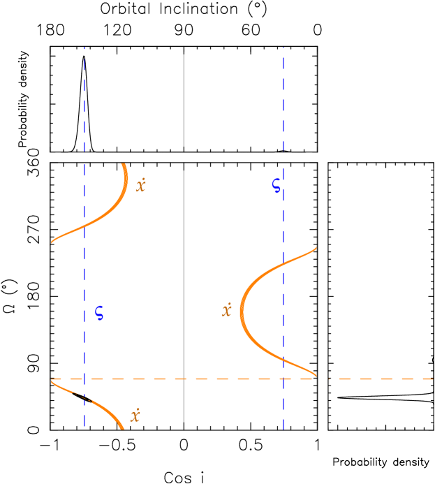
Figure 5: Orbital orientation constraints for PSR J2234+0611. In the main square panel we display the full $\cos i$-$\Omega$ plane; this has a priori a constant probability density for randomly aligned systems. The black contours include 68.23 and 95.44% of the total probability density function (pdf) derived from a 3-dimensional $\chi^{2}$ map of $\cos i$-$\Omega$-$M_{\rm tot}$ space using the DDK model with the additional assumption that GR is the correct theory of gravity. The dashed orange line indicates the PA of the proper motion of the system ($\Theta_{\mu}\,=\,69.0(1)\,\deg$). The dashed blue line indicates the $\varsigma$ assumed in our DDFWHE model; the solid orange lines indicate the regions that are consistent with the nominal and $\pm\,1-\sigma$ measurements of $\dot{x}$ obtained in that model (see Table 2). The $\varsigma$ and $\dot{x}$ constraints predict well the location of the region(s) of high probability but provide no distinction between the four locations where they cross (these are listed in Table 3); this can only be done using the DDK model (see text for details). The side panels display the 1-d pdfs for $\cos i$ (top) and $\Omega$ (right).

3.6 Secular change of the projected semimajor axis

As seen in Table 2, both the DDGR and DDFWHE timing solutions contain a precise measurement of a change in the projected semi-major axis ($\mathrm{x=a\sin i}$ where a is the semi-major axis and i is the orbital inclination) of the pulsar’s orbit, $\dot{x}\,=\,-2.79(7)\times 10^{-14}\,\rm lt-s\,s^{-1}$, thus $(\dot{x}/x)^{\rm obs}\,=\,-1.99(5)\times 10^{-15}\,\rm s^{-1}$. Following Lorimer & Kramer (2004), the observed change in $\dot{x}$ can, in the absence of a third object in the system, be written in terms of various contributions as:

$$\left(\frac{\dot{x}}{x}\right)^{\rm obs}\,=\,\left(\frac{\dot{x}}{x}\right)^{\rm k}\,+\,\left(\frac{\dot{x}}{x}\right)^{\rm GW}\,+\,\frac{d\epsilon_{A}}{dt}\,-\,\frac{\dot{D}}{D}\,+\,\left(\frac{\dot{x}}{x}\right)^{\dot{m}}\,+\,\left(\frac{\dot{x}}{x}\right)^{\rm SO}.$$ (8)

The first term is caused by the changing geometry due to the motion of the system relative to the Earth, it is given by (Kopeikin, 1995):

$$\dot{x}_{\rm k}=x\mu\cot i\sin(\Theta_{\mu}-\Omega),$$ (9)

where we have, again, re-written the terms as in Freire et al. (2011), except for the latter’s negative sign, so that we are in the right-handed convention being used in the DDK model. As we will see below, this is the only term that can account for the observations.

The second term is from the decrease of the size of the orbit caused by gravitational wave emission; this is given by

$$\left(\frac{\dot{x}}{x}\right)^{\rm GW}\,=\,\frac{2}{3}\frac{\dot{P}_{\rm b,GW}}{P_{\rm b}}\,=\,-6.31\times\,10^{-24}\,\rm s^{-1},$$ (10)

where we used the predicted $\dot{P}_{\rm b,GW}$ from the DDGR solution. This is more than eight orders of magnitude smaller than the measured value.

The third term, caused by aberration, is proportional to the geodetic precession rate for the pulsar, this is given by Barker & O’Connell (1975) as:

$$\Omega_{\rm geod}\,=\,\left(\frac{2\pi}{P_{\rm b}}\right)^{5/3}T_{\odot}^{2/3}\frac{1}{1-e^{2}}\frac{M_{c}(4M_{\rm tot}-M_{c})}{2M_{\rm tot}^{4/3}},$$ (11)

the result for PSR J2234+0611 is $\Omega^{\rm geod}\,=\,5.6\,\times\,10^{-14}\,\rm rad\,s^{-1}$, i.e., the geodetic precession cycle has a length of 3.6 Myr. The aberration contribution to $\dot{x}$ is then given by (Damour & Taylor, 1992):

$$\frac{d\epsilon_{A}}{dt}\,=\,\frac{P}{P_{b}}\frac{\Omega^{\rm geod}}{\sqrt{1-e^{2}}}\frac{\cot\lambda\sin 2\eta+\cot i\cos\eta}{\sin\lambda},$$ (12)

where $\eta$ and $\lambda$ are the polar coordinates of the pulsar’s spin. For PSR J2234+0611, the non-geometric factors (the first two fractions in the equation above) amount to $-7.28\,\times\,10^{-23}\rm\,s^{-1}$, making this term about 8 orders of magnitude smaller than the observed value.

The fourth term, $-\dot{D}/D\,=\,1.541\,\times\,10^{-18}\,s^{-1}$, is three orders of magnitude smaller than the observed effect.

The fifth term can be derived from eq. 10, with the orbital variability given by eq. 3, from this we obtain $(\dot{x}/x)^{\dot{m}}\,=\,2.53\,\times\,10^{-21}\rm\,s^{-1}$, which is also extremely small.

Finally, the sixth term is due to changes in the orbital plane of the system from spin-orbit coupling; these are extremely small in such a wide system.

Since the first term in eq. 8 is the only measurable contribution to $\dot{x}_{\rm obs}$, we will now assume that the latter is described by eq. 9. Using that equation, we can combine $\dot{x}_{\rm obs}$ with the Shapiro delay to constrain the system geometry as shown in Figure 5. The orange lines show the $\cos i$ and $\Omega$ that are consistent with the measured $\dot{x}$ while the dashed blue lines show the $\cos i$ compatible with the assumed $\varsigma$. These cross in four locations, listed in Table 3; these represent the four possible orbital orientations of the system according to the DDK and DDFWHE timing solutions.

3.7 Annual orbital parallax

For most pulsars where these constraints are available, we cannot eliminate the degeneracy implied by these four $i$-$\Omega$ solutions. However, if the binary system is relatively nearby and has a high timing precision, then apart from the secular variation of $\omega$ ($\dot{\omega}_{\rm obs}$) and $x$ ($\dot{x}_{\rm obs}$) there are yearly cyclical variations in these parameters caused by Earth’s orbit around the Sun (Kopeikin, 1996). These are taken into account in the DDK model.

In Table 3, we can see that the quality of the local $\chi^{2}$ minima are clearly not identical, being significantly better for solution 1 (this is the DDK solution presented in Table 2); the latter solution is significantly better than either the DDGR or the DDFWHE solutions. A possible reason for this is that we have detected the yearly cyclical variations of $x$ or $\omega$ or both. We quantify this statement in the next section.

4 Bayesian analysis of the system

Before we proceed, we emphasize that no single orbital model captures all features of the system in a self-consistent way. The DDGR and DDFWHE models over-estimate $M_{\rm tot}$ and $\dot{\omega}_{\rm rel}$ respectively (and because of that $M_{p}$ and $M_{c}$ as well) because they do not take into account $\dot{\omega}_{K}$. The DDK model captures the kinematic effects well and provides an accurate estimate of $\dot{\omega}_{\rm rel}$, but it has a larger than necessary uncertainty on $M_{c}$ (about $0.05\,M_{\odot}$, even with a fixed orbital inclination) because it uses a sub-optimal parameterization of the Shapiro delay and does not assume the validity of GR.

4.1 Mapping the $\Omega$-$\cos i$-$M_{c}$ space

Given all the correlations and caveats related to the different orbital models, and in order to better determine $M_{\rm tot}$, $M_{c}$, $M_{p}$, $i$, $\Omega$, their uncertainties and correlations, we have made a self-consistent $\chi^{2}$ map of the $\Omega$-$\cos i$-$M_{\rm tot}$ space using the DDK orbital solution with the assumption that GR is the correct theory of gravity. These parameters are chosen because they have a priori a constant probability density for randomly aligned orbits.

For each point in the grid of $i$, $\Omega$, and $M_{\rm tot}$ values, we hold $\Omega$ and $i$ fixed in the DDK model (from this it estimates all kinematic effects) and derive other relevant post-Keplerian parameters from the known mass function, $i$ and $M_{\rm tot}$ (M2; OMDOT and GAMMA) using the GR equations. All these parameters are fixed inputs to the DDK model used to do the timing analysis for that grid point. The Einstein delay (GAMMA) must be calculated and used in the fit because, for wide binary pulsars like PSR J2234+0611, it is strongly correlated with $\dot{x}$ in the DDFWHE model and with $\Omega$ in the DDK model (see Ridolfi et al. 2018, in preparation). We then run tempo, fitting for all other timing parameters not mentioned above, recording the value of $\chi^{2}$ for each combination of $\Omega$, $\cos i$ and $M_{\rm tot}$.

Given the computational expense, our $\chi^{2}$ map does not cover the full space; it consists instead of four disconnected regions around the four local $\chi^{2}$ minima listed in Table 3; the $\cos i$ and $\Omega$ bounds sampled around these minima are also listed there. These variables are sampled with step sizes of 0.004 and $0.2\,\deg$, respectively. For each grid section, we mapped the third variable, $M_{tot}$ from 1.641$M_{\odot}$ to 1.731$M_{\odot}$ with a step size of 0.0006$M_{\odot}$. The quality of the fits in the regions outside these bounds are extremely low, for that reason those regions were not sampled.

The resulting 3-D grids of $\chi^{2}$ values are then used to calculate a 3-dimensional probability density function (pdf) for $\Omega,\cos i,M_{\rm tot}$, as discussed by Splaver et al. (2002):

$$p(\Omega,\cos i,M_{\rm tot})\propto e^{(\chi^{2}_{\rm min}-\chi^{2})/2},$$ (13)

where $\chi^{2}_{\rm min}$ is the lowest $\chi^{2}$ of the whole grid.

This 3-D pdf is then projected onto two planes: the $\cos i-M_{c}$ plane and derived $M_{c}$-$M_{p}$ plane (see contours in the main panels in figure 4) and the $\cos i$-$\Omega$ plane (see contours in main panel of figure 5). It is also projected along three axes, $\cos i$ (top left side panels in figures 4 and 5), $M_{c}$ (and derived $M_{p}$, see top right and right side panels in figure 4) and $\Omega$ (depicted in the right side panel of figure 5).

4.2 Results of the Bayesian analysis

The resulting 1-D pdfs show that, as hinted by the $\chi^{2}$ values in Table 3, the probabilities for the four $i$-$\Omega$ solutions are far from identical. The solution with the lowest $\chi^{2}$ (number 1) is preferred, with a total probability of 98.786%. The second most likely solution (number 2), has a total probability of 1.214%, it is still visible in the side panels of Fig. 5 as a separate peak with very small amplitude. Solutions 3 and 4 have probabilities that are too small for our numerical precision, being thus definitively excluded. The discrimination between solutions 1 and 2, i.e., between the two possible values of $i$ and $\Omega$ does not yet reach a statistical significance equivalent to 3$\sigma$, but they imply that the absolute orbital orientation of the system will be precisely known in the near future. Despite the fact that we cannot yet point out a single solution to equivalent 3-$\sigma$ significance, the exclusion of two of the solutions to high significance implies a significant detection of the annual orbital parallax.

The values derived for the quantities we set out to determine are: $i=138.7^{+2.5}_{-2.2}\,\deg$ (68.27 % C. L.), $138.7^{+5.1}_{-4.2}\deg$ (95.45 % C. L.), $\Omega\,=\,43.7^{+2.3}_{-2.2}\deg$ (68.27 % C. L.) and $43.7^{+5.2}_{-4.4}\deg$ (95.45 % C. L.). In Fig. 5, we see a fine correlation between $i$ and $\Omega$, which is a direct consequence of the precisely measured $\dot{x}$.

For the component masses, the situation is very clear: both solutions with measurable probability have the same total mass, $M_{\rm tot}\,=\,1.6518^{+0.0033}_{-0.0035}\,\rm M_{\odot}$ (68.27 % C. L.), $1.6518^{+0.0066}_{-0.0070}\,\rm M_{\odot}$ (95.45 % C. L.). For the component masses we obtain $M_{c}\,=\,0.298^{+0.015}_{-0.012}\,\rm M_{\odot}$ (68.27 % C. L.), $0.298^{+0.034}_{-0.021}\,\rm M_{\odot}$ (95.45 % C. L.), $M_{p}\,=\,1.353^{+0.014}_{-0.017}\,\rm M_{\odot}$ (68.27 % C. L.) and $1.353^{+0.025}_{-0.040}\,\rm M_{\odot}$ (95.45 % C. L.). The fine $\Omega$-$i$ correlation also affects the mass measurements: for values of $\Omega$ closer to $\Theta_{\mu}$, the more face-on inclinations result in a more massive companion and a less massive pulsar.

The measurements made by the Bayesian analysis are in good agreement with the values inferred by the results in Section 3. For example, the total mass is well described by the $\dot{\omega}$ of the DDK solution, as it must since we used the latter model to map the masses assuming GR. The individual masses are well described by the intersection of the latter constraint with the $h_{3}$ of the DDFWHE solution. The constraints these impose on the range of inclinations plus the constraints imposed by the detection of $\dot{x}$ in the DDGR/DDFWHE solutions provide a good description of the range of $\Omega$, plus its strong correlation with $i$ near the best DDK solution.

5 Implications

The mass of PSR J2234+0611 is very similar to that of PSR J1807$-$2500B in the globular cluster NGC 6544 ($M_{p}\,=\,1.3655(21)\,M_{\odot}$, Lynch et al. 2012), PSR J1713+0737 ($M_{p}\,=\,1.33^{+0.09}_{-0.08}\,M_{\odot}$, Arzoumanian et al. 2018 or $M_{p}\,=\,1.35(7)\,M_{\odot}$, Desvignes et al. 2016). Until recently these would have been considered unusually small masses for a fully recycled pulsar. However, recent measurements show that two other fully recycled pulsars might be even less massive: PSR J1918$-$0642 ($M_{p}\,=\,1.29^{+0.10}_{-0.09}\,M_{\odot}$ Arzoumanian et al. 2018) and PSR J0514$-$4002A, a 5-ms pulsar located in the globular cluster NGC 1851 ($M_{p}\,=\,1.25^{+0.06}_{-0.05}\,M_{\odot}$, see Ridolfi et al. 2018, in preparation).

Such low masses are interesting because they can constrain the efficiency of the recycling process (for a detailed discussion see Antoniadis et al., 2012, ; an update of that discussion is presented by Ridolfi et al., in prep). If PSR J2234+0611 indeed descended from a typical LMXB (section 5.1), then the system parameters reported here imply, following the arguments presented by Antoniadis et al. (2016a), a mass-accretion efficiency (the fraction of mass lost by the donor that is accreted onto the neutron star) of at most $\sim 30\%$ for an initial pulsar mass $\leq 1.17$ M_⊙, or $\sim 6\%$ for a more typical initial mass of 1.35 M_⊙.

5.1 Formation of eccentric MSPs

Our analysis of PSR J2234$+$0611 is informed by previous work on two other eccentric binary systems, PSRs J1946$+$3417 and J1950$+$2414. Mass measurements of these three pulsars can be combined to constrain theories of formation for eccentric binary MSPs. The rotation-delayed accretion induced collapse (RD-AIC) hypothesis presented by Freire & Tauris (2014) for the formation of the eccentric MSPs has been excluded already by the mass measurement for PSR J1946+3417 presented in Barr et al. (2017): the mass of that pulsar ($M_{p}\,=\,1.828(22)\,M_{\odot}$) is too large to have resulted from the collapse of a massive WD.

The RD-AIC theory could in principle generate larger MSP masses if we allow for differential rotation of the massive WD progenitor to the MSP: With differential rotation WDs can be much more massive than the $\sim\,1.48\,M_{\odot}$ upper mass limit for rigidly rotating WDs. However, even in such a case the systems produced by RD-AIC would still have small peculiar velocities, otherwise the range of observed orbital eccentricities wouldn’t be as small as the observed range (see details in Freire & Tauris 2014). Such a possibility is difficult to reconcile with the large peculiar velocity measured for PSR J1946+3417 (in particular its large vertical velocity relative to the Galaxy, see Barr et al. 2017) and the observed velocity of PSR J2234+0611 (Antoniadis et al., 2016a).

The large mass of PSR J1946+3417 is consistent with the hypothesis proposed by Jiang et al. (2015), which is also based on an instantaneous loss of binding energy of the more massive component. However, in this hypothesis the more massive component starts as a massive MSP. As it spins down, the centrifugal support is steadily reduced, causing a slow but steady increase in the central pressure with time, until a critical threshold is reached and the phase transition happens, presumably forming a quark star or some other type of exotic object that is still observable as a MSP. The sudden decrease in mass (owing to the larger binding energy of the new exotic remnant) results in the large orbital eccentricity. Other properties of PSR J1946+3417, like the large vertical velocity relative to the Galactic disk, are also consistent with this hypothesis, since the original system already shared the large velocity (relative to typical stars in the Galactic disk) typical of MSP-WD binaries. However, if there is a single pressure threshold for this phase transition, the masses observed for the MSPs in these eccentric systems should lie in a relatively narrow range (which is nevertheless finite because of differences in the spin periods, which would result in different NS masses for the same central pressure at which the phase transition occurs).

The masses measured for PSR J2234+0611 ($1.35\,\rm M_{\odot}$) and for PSR J1950+2414 ($M_{p}\,=\,1.495(24)\,M_{\odot}$, Zhu et al. 2018, in preparation) are inconsistent with this hypothesis, since they are much smaller than the mass observed for PSR J1946+3417 - clearly, a single pressure threshold for a phase transition does not provide a good description of these systems. Indeed, the observed MSP masses within this class appear to be as broad as observed for the general MSP population (Özel & Freire, 2016; Antoniadis et al., 2016b).

All measurements thus far are consistent with the expectations of the hypothesis proposed by Antoniadis (2014). This proposes that the orbital eccentricity is caused by material ejected from the companion due to unstable hydrogen shell burning. This hypothesis predicts that the MSPs in these systems should have a range of masses and Galactic velocities similar to those of the general MSP population; the observations are thus far consistent with this prediction.

Regarding the companions to the MSPs in these systems, all hypotheses advanced to date predict that they should be Helium white dwarfs with masses similar to what should be expected from the Tauris & Savonije (1999) relation. For PSRs J1946$+$3417, J1950$+$2414, and J2234$+$0611 the mass ranges predicted by this relation are 0.275–0.303, 0.268–0.296, and 0.281–0.310, respectively. In the case of PSR J2234+0611, our measured WD mass is in agreement with that prediction. For PSR J1946+3417, the companion mass $M_{c}\,=\,0.2556(19)\,M_{\odot}$ is marginally consistent with this expectation, being lighter than expected. The companion of PSR J1950+2414 has a mass ($M_{c}\,=\,0.280_{-0.004}^{+0.006}\,M_{\odot}$) that is also well within the range expected by Tauris & Savonije (1999) for its orbital period. We note that within the context of the CB disk scenario, depending on the lifetime and mass of the disk, there could be a significant (up to $\sim 10\%$) reduction of the orbital separation. This effect would result in somewhat larger masses for a given orbital period, compared to the Tauris & Savonije (1999) relation — the opposite of what is observed for PSR J1946+3417.

5.2 White dwarf properties

The distance to PSR J2234+0611 is very well measured through the detection of timing parallax, $\mathrm{\varpi=1.03(4)}\,\rm mas$. This corresponds to a distance $d\,=\,0.97(4)$ kpc. The uncertainty of 40 pc for J2234+0611 places it among the best measured pulsar distances.

The distance estimate will improve further in the near future. As the timing baseline $T$ increases, the precision of $\dot{P}_{\rm b,obs}$ will also improve quickly. This will result in an additional precise distance estimate from the inversion of eq. 2, which will only be limited by knowledge of the Galactic potential. Measurements of this distance can be corroborated by VLBI campaigns. The component masses will also improve significantly, particularly the total mass; for the individual masses significant improvements will depend on advances in timing precision.

The precise distance and mass estimates presented here, together with the spectroscopic constraints on the WD atmospheric properties, transform the system into a laboratory for testing WD physics. As discussed in detail in Antoniadis et al. (2016a), the aforementioned measurements yield a radius estimate of $R_{\rm WD}=0.024_{-0.002}^{+0.004}$ R_⊙ and a surface gravity of $\log g=7.11_{-0.16}^{0.08}$ dex, both of which are model-independent. This is important for two reasons: firstly, PSR J2234+0611 is only the second system after PSR J1909$-$3744 for which independent atmospheric parameters can be obtained (Antoniadis et al., 2016a). Second, the surface temperature of $T_{\rm eff}\simeq 8600$ K obtained from atmospheric modeling, indicate that the WD envelope is convective. Spectroscopic 1D models for cool convective atmospheres are suspected to produce spurious results, but quantitative estimates and empirical corrections are difficult to obtain due to the lack of measurements. For both these reasons, PSR J2234+0611 becomes particularly important for calibrating atmospheric models. Currently, the precision of such tests is severely limited by the poor quality of the optical spectra, but could be improved significantly with further optical observations.

In addition, PSR J2234+0611 can also be used to test the predictions of WD mass-radius relations. One of the main remaining uncertainties in low-mass WD cooling models is the size of the hydrogen envelope that surrounds the degenerate Helium core. The latter can significantly affect the stellar radius, as well as the main energy source (residual hydrogen shell burning vs thermal cooling) and, consequently, the cooling age. Here again, our estimates are broadly consistent with the predictions for thin-envelope models, but a detailed test is limited by measurement uncertainties of the WD atmospheric parameters (see Antoniadis et al., 2016a, for details). For PSR J2234+0611, a future precision measurement of its envelope size is also important for probing its formation history, since the thin-shell instabilities on the proto-WD required for creating a CB disk, are also expected to reduce significantly the size of the WD envelope (see Istrate et al., 2014, 2016; Antoniadis et al., 2016a, and references therein).

Last but not least, PSR J2234+0611 is within a few 100 K from the ZZ-Ceti instability strip for low-mass WDs. Kilic et al. (2018) recently reported on photometric observations of the system and found no pulsations. Consequently, the improved mass estimate reported in this work can further constrain the instability mechanism and the structure of WD envelopes (see Figure  5 in Kilic et al., 2018, and references therein for details).

6 Conclusions

We have reported the timing solution for PSR J2234$+$0611, a 3.6-ms pulsar in an eccentric (e = 0.13), 32-day orbit with a He white dwarf. The pulsar is bright (especially with Arecibo) and has a narrow pulse and therefore has excellent timing precision. It was added to pulsar timing array efforts soon after discovery and therefore is observed regularly. The exceptional timing properties of this pulsar, its eccentric orbit, and the optical detection has allowed the precise measurement of an unprecedented number of parameters, indeed, this is the first binary pulsar where we know the precise 3-D location and 3-D velocity, the full 3-D orientation of the orbit and, on top of that, we are able to determine precise masses. To our knowledge, no other binary pulsar has such precisely determined overall geometry.

We have compared the characteristics of this pulsar to those expected from various theories for the eccentric MSP systems and show that the only viable remaining theory is one where mass-loss occurs due to unstable shell-hydrogen burning in the proto-WD (Istrate et al., 2014; Antoniadis, 2015; Istrate et al., 2016). We expect that this MSP system will be useful for constraining white dwarf models, given its well measured distance, white dwarf mass, and optically detectable companion.

References

- Alpar et al. (1982) Alpar, M. A., Cheng, A. F., Ruderman, M. A., & Shaham, J. 1982, Nature, 300, 728
- Antoniadis (2014) Antoniadis, J. 2014, ApJ, 797, L24
- Antoniadis (2015) Antoniadis, J. 2015, in Astrophysics and Space Science Proceedings, Vol. 40, Gravitational Wave Astrophysics, ed. C. F. Sopuerta, 1
- Antoniadis et al. (2016a) Antoniadis, J., Kaplan, D. L., Stovall, K., et al. 2016a, ApJ, 830, 36
- Antoniadis et al. (2016b) Antoniadis, J., Tauris, T. M., Ozel, F., et al. 2016b, ArXiv e-prints, arXiv:1605.01665 [astro-ph.HE]
- Antoniadis et al. (2012) Antoniadis, J., van Kerkwijk, M. H., Koester, D., et al. 2012, MNRAS, 423, 3316
- Arzoumanian et al. (2018) Arzoumanian, Z., Brazier, A., Burke-Spolaor, S., et al. 2018, ApJS, 235, 37
- Barker & O’Connell (1975) Barker, B. M., & O’Connell, R. F. 1975, Phys. Rev. D, 12, 329
- Barr et al. (2017) Barr, E. D., Freire, P. C. C., Kramer, M., et al. 2017, MNRAS, 465, 1711
- Barr et al. (2013) Barr, E. D., Champion, D. J., Kramer, M., et al. 2013, MNRAS, 435, 2234
- Camilo (1995) Camilo, F. 1995, PhD thesis, PRINCETON UNIVERSITY.
- Camilo et al. (2015) Camilo, F., Kerr, M., Ray, P. S., et al. 2015, ApJ, 810, 85
- Champion et al. (2008) Champion, D. J., Ransom, S. M., Lazarus, P., et al. 2008, Science, 320, 1309
- Cognard et al. (2017) Cognard, I., Freire, P. C. C., Guillemot, L., et al. 2017, ApJ, 844, 128
- Cordes & Lazio (2002) Cordes, J. M., & Lazio, T. J. W. 2002, ArXiv Astrophysics e-prints, astro-ph/0207156
- Damour & Deruelle (1985) Damour, T., & Deruelle, N. 1985, Ann. Inst. Henri Poincaré Phys. Théor., Vol. 43, No. 1, p. 107 - 132, 43, 107
- Damour & Deruelle (1986) —. 1986, Ann. Inst. Henri Poincaré Phys. Théor., Vol. 44, No. 3, p. 263 - 292, 44, 263
- Damour & Taylor (1991) Damour, T., & Taylor, J. H. 1991, ApJ, 366, 501
- Damour & Taylor (1992) —. 1992, Phys. Rev. D, 45, 1840
- Demorest et al. (2013) Demorest, P. B., Ferdman, R. D., Gonzalez, M. E., et al. 2013, ApJ, 762, 94
- Deneva et al. (2013) Deneva, J. S., Stovall, K., McLaughlin, M. A., et al. 2013, ApJ, 775, 51
- Desvignes et al. (2016) Desvignes, G., Caballero, R. N., Lentati, L., et al. 2016, MNRAS, 458, 3341
- Edwards & Bailes (2001) Edwards, R. T., & Bailes, M. 2001, ApJ, 553, 801
- Edwards et al. (2006) Edwards, R. T., Hobbs, G. B., & Manchester, R. N. 2006, MNRAS, 372, 1549
- Freire & Tauris (2014) Freire, P. C. C., & Tauris, T. M. 2014, MNRAS, 438, L86
- Freire & Wex (2010) Freire, P. C. C., & Wex, N. 2010, MNRAS, 409, 199
- Freire et al. (2011) Freire, P. C. C., Bassa, C. G., Wex, N., et al. 2011, MNRAS, 412, 2763
- Gentile et al. (2018) Gentile, P. A., McLaughlin, M. A., Demorest, P. B., et al. 2018, ApJ, 862, 47
- Gonzalez et al. (2011) Gonzalez, M. E., Stairs, I. H., Ferdman, R. D., et al. 2011, ApJ, 743, 102
- Gravity Collaboration et al. (2018) Gravity Collaboration, Abuter, R., Amorim, A., et al. 2018, A&A, 615, L15
- Hotan et al. (2004) Hotan, A. W., van Straten, W., & Manchester, R. N. 2004, PASA, 21, 302
- Istrate et al. (2016) Istrate, A. G., Marchant, P., Tauris, T. M., et al. 2016, A&A, 595, A35
- Istrate et al. (2014) Istrate, A. G., Tauris, T. M., Langer, N., & Antoniadis, J. 2014, A&A, 571, L3
- Jiang et al. (2015) Jiang, L., Li, X.-D., Dey, J., & Dey, M. 2015, ApJ, 807, 41
- Kilic et al. (2018) Kilic, M., Hermes, J. J., Córsico, A. H., et al. 2018, MNRAS, 479, 1267
- Knispel et al. (2015) Knispel, B., Lyne, A. G., Stappers, B. W., et al. 2015, ApJ, 806, 140
- Kopeikin (1995) Kopeikin, S. M. 1995, ApJ, 439, L5
- Kopeikin (1996) —. 1996, ApJ, 467, L93
- Lazaridis et al. (2009) Lazaridis, K., Wex, N., Jessner, A., et al. 2009, MNRAS, 400, 805
- Lorimer & Kramer (2004) Lorimer, D. R., & Kramer, M. 2004, Handbook of Pulsar Astronomy
- Lynch et al. (2012) Lynch, R. S., Freire, P. C. C., Ransom, S. M., & Jacoby, B. A. 2012, ApJ, 745, 109
- McGaugh (2018) McGaugh, S. 2018, ArXiv e-prints, arXiv:1808.09435
- McMillan (2017) McMillan, P. J. 2017, MNRAS, 465, 76
- Nice et al. (2015) Nice, D., Demorest, P., Stairs, I., et al. 2015, Tempo, Astrophysics Source Code Library, ascl:1509.002
- Octau et al. (2018) Octau, F., Cognard, I., Guillemot, L., et al. 2018, A&A, 612, A78
- Özel & Freire (2016) Özel, F., & Freire, P. 2016, ARA&A, 54, 401
- Phinney (1992) Phinney, E. S. 1992, Philosophical Transactions of the Royal Society of London Series A, 341, 39
- Radhakrishnan & Srinivasan (1982) Radhakrishnan, V., & Srinivasan, G. 1982, Current Science, 51, 1096
- Ransom (2011) Ransom, S. 2011, PRESTO: PulsaR Exploration and Search TOolkit, Astrophysics Source Code Library, ascl:1107.017
- Ransom (2001) Ransom, S. M. 2001, PhD thesis, Harvard University
- Robertson (1938) Robertson, H. P. 1938, Ann. Math., 38, 101
- Shklovskii (1970) Shklovskii, I. S. 1970, Soviet Ast., 13, 562
- Splaver et al. (2002) Splaver, E. M., Nice, D. J., Arzoumanian, Z., et al. 2002, ApJ, 581, 509
- Tauris & Savonije (1999) Tauris, T. M., & Savonije, G. J. 1999, A&A, 350, 928
- Taylor & Weisberg (1982) Taylor, J. H., & Weisberg, J. M. 1982, ApJ, 253, 908
- The NANOGrav Collaboration et al. (2015) The NANOGrav Collaboration, Arzoumanian, Z., Brazier, A., et al. 2015, ApJ, 813, 65
- Weisberg & Huang (2016) Weisberg, J. M., & Huang, Y. 2016, ApJ, 829, 55
- Yao et al. (2017) Yao, J. M., Manchester, R. N., & Wang, N. 2017, ApJ, 835, 29
- Zahn (1977) Zahn, J.-P. 1977, A&A, 57, 383