\lettrine[lines=1]Extragalactic Searches
for
Dark Matter Annihilation
Abstract
We are at the dawn of a data-driven era in astrophysics and cosmology. A large number of ongoing and forthcoming experiments combined with an increasingly open approach to data availability offer great potential in unlocking some of the deepest mysteries of the Universe. Among these is understanding the nature of dark matter (DM)—one of the major unsolved problems in particle physics. Characterizing DM through its astrophysical signatures will require a robust understanding of its distribution in the sky and the use of novel statistical methods.
The first part of this thesis describes the implementation of a novel statistical technique which leverages the “clumpiness” of photons originating from point sources (PSs) to derive the properties of PS populations hidden in astrophysical datasets. This is applied to data from the Fermi satellite at high latitudes () to characterize the contribution of PSs of extragalactic origin. We find that the majority of extragalactic gamma-ray emission can be ascribed to unresolved PSs having properties consistent with known sources such as active galactic nuclei. This leaves considerably less room for significant dark matter contribution.
The second part of this thesis poses the question: “what is the best way to look for annihilating dark matter in extragalactic sources?” and attempts to answer it by constructing a pipeline to robustly map out the distribution of dark matter outside the Milky Way using galaxy group catalogs. This framework is then applied to Fermi data and existing group catalogs to search for annihilating dark matter in extragalactic galaxies and clusters.
September 2018 \adviserMariangela Lisanti \departmentPhysics
Chapter 1 Introduction
The nature of dark matter (DM) remains one of the major unsolved problems in physics. Originally inferred through its gravitational influence on galaxies and clusters, a rich body of evidence has accumulated over the last four decades firmly establishing its existence. All of the evidence, however, comes from inferring dark matter’s presence solely through its gravitational effects. Many open questions remain: Does dark matter consist of a fundamental particle? If so, what is its mass? Could there be an entire dark sector, akin to the Standard Model (SM)? How does dark matter interact with the SM? The quest to answer these questions drives a huge collective effort that draws from a rich body of theoretical and experimental work, as well as major input from computational and numerical studies. We are currently at the dawn of a data-driven era in astrophysics and cosmology—a large number of ongoing and forthcoming experiments, both in the lab and in the sky, combined with an increasingly open approach to data availability, offer great potential in elucidating the nature of dark matter.
Dark matter plays a central role in many subfields of particle physics, astrophysics and cosmology. Understanding its nature and interactions would have far reaching consequences in those fields by providing major insights into fundamental physics beyond the Standard Model as well as elucidating the evolution of our Universe and the formation of structures within it.
This introduction is organized as follows. In Sec. 1.1, I will summarize the large body of evidence pointing to the existence of dark matter, occasionally touching upon relevant historical developments. In Sec. 1.2, I will describe possible explanations for the particle nature of dark matter and various detection schemes, focusing on DM thermally produced in the early Universe and specifically Weakly Interacting Massive Particles (WIMPs). Section 1.3 will focus on the effort to detect and characterize WIMPs through their astrophysical signatures, in particular using gamma-ray data. I will briefly summarize the theoretical and experimental tools available to us in these searches. Finally, in Sec. 1.4, I will describe the organization of the rest of this thesis. This chapter partially draws from a number of excellent review articles on the topic which the reader is referred to for further details. Refs. [1, 2] provide recent, comprehensive reviews of dark matter physics. Ref. [3] reviews indirect detection, which will be the main focus of this thesis. Finally, Ref. [4] provides a thorough overview of the history of the field.
1.1 Evidence for Dark Matter
Although the study of dark matter had its inception and development in the 20th century, the interplay between theory and observation in making the unknown knowable goes back much earlier. For example, the Aristotelian view of an immutable Universe with the Earth at its center offered a clean framework that did not call for additional celestial objects, and was the orthodox viewpoint until Renaissance astronomers conclusively refuted it with observations. Galileo was able to leverage new technological developments and make observations that arguably played the largest role in this. After pioneering the development of the telescope, he was able to understand the make-up of the Milky Way as consisting of individual stars rather than diffuse clouds, observe Saturn’s rings and discover Jupiter’s four largest moons. These observations are very much in the spirit of modern dark matter searches—demonstrating that the Universe can contain invisible forms of matter, and that scientific inquiry and technological developments can play a big role in revealing them to us.
Evidence for some yet-unknown form of matter started piling up in the early 19th century. In 1922, Dutch astronomer Jacobus Kapteyn wrote down for the first time a predictive model for the distribution of matter in the Milky Way, describing the stars as particles in a virialized system [5] and using this model to obtain the local matter density in terms of the observed stellar mass. Kapteyn’s student Jan Oort [6] and others [7] were able to derive estimates for the local matter density, in some cases seeing excesses above the observed luminous mass. Astronomers during this time reckoned with the existence of missing matter in the Universe, in some cases explicitly using the term dark matter [5] and positing that it could potentially be accounted for by the extrapolation of the stellar luminosity function down to very faint stars [6].
In 1933, Swiss-American astronomer Fritz Zwicky studied redshift data for galaxy clusters collected by Hubble and Humason [8], using estimates of the velocity dispersions in eight galaxies within the Coma cluster to estimate its mass through the virial theorem [9]. Zwicky obtained a theoretical prediction for the dispersion by using the number of observed galaxies, average mass of a galaxy and its extent, finding a value of 80 km s-1. This was in stark conflict with the observed line-of-sight velocity dispersion of 1000 km s-1. Although Zwicky’s work made use of an estimate of the Hubble constant that was a factor of 8 too big compared to the current accepted value, the large discrepancy between the observed and expected values pointed to the existence of unaccounted-for matter in the Coma system. Zwicky himself concluded that “If this would be confirmed, we would get the surprising result that dark matter is present in much greater amount than luminous matter.” An analysis of the Virgo cluster by Sinclair Smith in 1936 again pointed to a very high mass-to-light ratio in that system. In either case, the astronomers put forward potential explanations in terms of diffuse clouds of internebular material [10].
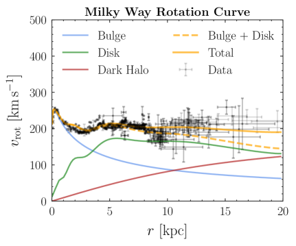
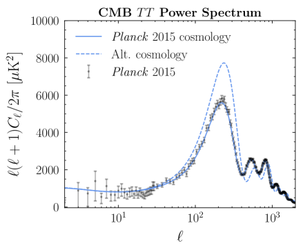
Although this presented a conundrum, there was widespread consensus within the astronomical community that more information would be needed to understand what was going on. Historically, velocity rotation curves—the circular velocity profiles of stars in a galaxy as a function of the distance from the galactic center—did the most to convince the scientific community of the existence of large amounts of non-luminous matter in galaxies. The basic idea here is as follows. Standard Newtonian theory dictates that the circular velocity of stars is given by , where is the radial distance, the mass enclosed within radius and the universal gravitational constant. In the region beyond the galactic disk (which defines the observed extent of a given galaxy), we expect the enclosed mass to be constant, and consequently the circular velocity to fall as . Measurements started in the late 1930s with Babcock’s observations of the rotation curve of M31 (Andromeda) out to about 20 kpc from its center [11]. Technological advancements over the next few decades enabled more accurate measurements. In the 1970s, Kent Ford, Vera Rubin and others observed in galaxies such as M31 and M33 as well as the Milky Way the approximate flattening of rotation curves at distances extending well beyond the baryonic disk [12, 13]. The implications of these observations for the missing mass problem were realized soon after [14, 15]. Flat rotation curves indicated that the mass contained in a galaxy continues to increase as beyond the extent of the visible matter, in the form of unobserved “dark” matter whose density can be inferred to roughly scale as . The left panel of Fig. 1.1 shows the measured rotation curves for the Milky Way compiled in Ref. [16] compared with theoretical expectations from bulge- and disk-like components (blue and green lines, respectively) inferred from baryonic matter, as well as an additional dark matter component from a spherical, isothermal dark matter halo (red line). The rotation curve for the baryonic-only component (disk + bulge) is shown as the dashed yellow line, and the total rotation curve including the dark halo is shown as the solid yellow line. It can clearly be seen that the additional dark halo component is required to match the observed data at larger radii kpc. The descriptions of the individual components shown are provided in Ref. [16].
While astrophysical observations played a significant role historically in motivating the study of dark matter, modern cosmological data provides substantial evidence supporting its existence in our Universe. CDM, a phenomenological framework often referred to as the standard model of cosmology, contains dark energy () and cold dark matter (CDM) as essential ingredients. It is able to account for a plethora of cosmological observations, including the existence and structure of the cosmic microwave background (CMB) radiation, large-scale distribution of matter, accelerating expansion of the Universe and relic elemental abundances [17, 18]. In particular, the CMB, which is the imprint of photons that decoupled from the baryon-photon fluid in the Universe about 370,000 years ago and have been free-streaming ever since, provides irrefutable evidence for (non-baryonic) dark matter. The primary relevant observable is the angular scale of inhomogeneities in the temperature distribution (the angular power spectrum) of the CMB. The power spectrum largely consists of a set of peaks, each indicating an angular scale with a particularly large contribution to the temperature fluctuations. The leading physical effect behind these are acoustic oscillations in the baryon-photon fluid during photon decoupling. Early on, photons and baryons were electromagnetically coupled, and non-baryonic dark matter was responsible for generating gravitational potential wells that could pull in the baryon-photon fluid. The photon pressure acting against these wells gave rise to a tower of acoustic modes, imprinted in the CMB as characteristic peaks. While the detailed physics is somewhat nuanced***See Wayne Hu’s CMB tutorials for an excellent introduction: http://background.uchicago.edu/index.html., the relative heights of these peaks can provide information about the energy content of our Universe, including the relative composition of baryonic and non-baryonic (dark) matter. Very heuristically, the position of the first peak provides information about the curvature of the universe (and hence how much total “stuff” there is in it), while the second peak tells us how much of the matter is baryonic (ordinary matter). The third peak and its relative height can shed insights into the abundance of non-baryonic dark matter. Historically, the WMAP satellite, while not able to fully resolve the third peak, was already able to conclusively say that dark matter makes up the majority of the matter budget in the Universe, finding the baryon density and cold dark matter density [19]. Since then, Planck has been able to precisely measure eight peaks of the spectrum, finding and when additionally including the CMB -mode polarization auto- and cross-spectra ( and ). The right panel of Fig. 1.1 shows the Planck spectrum [20] along with the best-fit theoretical predictions (solid blue line), as well as predictions for a slightly altered cosmology and with a reduced dark matter density (dashed blue line), where striking differences from the measured spectrum can be seen.
The above classes of observational evidence or the existence of DM are by no means exhaustive—many other observations over a large range of scales support the existence of dark matter, including observations of the distribution of galaxies on large scales [22], weak [23] and strong lensing [24, 25] of background galaxies by foreground structure, and observations of merging clusters [26].
1.2 (Particle) Nature of Dark Matter
Although there exists a great deal of evidence for the existence of dark matter, its nature largely remains a mystery. These days, it is often implicitly assumed that when people are talking about detecting dark matter, say at a Xenon direct detection experiment or in gamma-ray data, they are referring to a dark matter particle. As touched upon above, this has by no means always been the case—early usage and references to dark matter usually referred to the existence of generic dark objects that would be too faint to be observed, such as dim stars or internebular material [10]. The transition in usage was a result of sociological changes within the particle physics and astrophysics communities, bringing the two closer after the missing mass problem had been firmly accepted in the 1970s. All evidence amassed since then is consistent with dark matter being a fundamental particle, or even the existence of an entire dark sector consisting of many particles with a rich set of properties and interactions. It should be noted however that there exist alternatives to particle dark matter that seek to explain the dynamical observations suggesting the existence of missing mass in the Universe. In particular, MOdified Newtonian Dynamics (MOND) [27, 28, 29] posits an alteration of Newtonian gravitation on larger scales and is successful in explaining the observed rotation curves as well as the empirical Tully-Fisher relation between the intrinsic luminosities and angular velocities of spiral galaxies [30]. While having some observational success, MOND and related theories [31] are (arguably) less successful at explaining observations on cluster and cosmological scales. See the reviews in Refs. [32, 33] for further details.
Within the Standard Model, neutrinos—by virtue of being stable (or very long-lived), electrically neutral particles that do not interacting strongly—contain some of the essential attributes for a particle dark matter candidate, and were considered a promising DM candidate from early on. Cosmological effects of neutrinos were explored throughout the 1960s and 1970s, pioneered by the work of Zeldovich and others [34, 35], and implications of massive neutrinos for the missing mass observed on (super-)galactic scales were discussed in the the late 1970s [36, 37]. Early simulations during the 1980s eventually showed that hot (relativistic) and cold (non-relativistic) particle dark matter would lead to very different outcomes for structure formation: in the former case leading to formation and collapse of larger structures (known as “top-down” structure formation), where in the latter case overdensities would seed larger structures, leading to hierarchical (known as “bottom-up”) structure formation. Neutrinos, by virtue of being very light thermal relics, would be extremely relativistic during structure formation and, combined with these simulations, early surveys of the local Universe were able to quickly discount them as dark matter candidates [38]. Nevertheless, neutrinos served as a gateway to understanding how potential new particles could affect observations on galactic, cluster and cosmological scales.
With no reason to be confined to the Standard Model, people turned to theories beyond the Standard Model that could explain DM. Supersymmetry (SUSY) posits that nature may contain a spacetime symmetry relating bosons and fermions, requiring that for every boson there must exist a fermion with the same quantum numbers (and vice versa) [39, 40]. This leads to the prediction of several new electrically neutral particles that are uncharged under the strong force. If some of these were stable, they could have played an important role in the history of our Universe and could conceivably make up (some portion of) the dark matter [41]. Supersymmetry took its modern form in a paper by Dimopolous and Georgi, who introduced the Minimal Supersymmetric Standard Model (MSSM) [42]. Here, superpartners of the boson, photon and two Higgses mix to form four particles, known today as neutralinos. Neutralinos have arguably been the most-discussed (particle) dark matter candidate [43], in part because supersymmetry—able to achieve gauge coupling unification and to solve the electroweak hierarchy problem—is motivated in its own right independent of the dark matter problem, and the existence of a viable DM candidate within SUSY is often seen as a desirable bonus.
Outside of SUSY, there is no shortage of viable particle DM candidates, including but not limited to axions [44, 45], sterile neutrinos [46, 47], light (sub-GeV) dark matter [48, 49] and fuzzy dark matter [50]. Such a wealth of possibilities exists in part because the most general observational constraints on the properties of particle DM are relatively mild. For example, the mass of the dominant DM component has only been constrained with orders of magnitude. In particular, observations constrain eV for bosonic dark matter [51] and keV for fermionic dark matter [52]. This is obtained from observations of DM halos around dwarf galaxies, imposing the requirement for particles to occupy a minimum phase-space volume according to the uncertainty principle for bosons and the Pauli exclusion principle for fermions. An upper limit of 1048 GeV comes from searches for microlensing signatures of MACHOS (Massive Astrophysical Compact Halo Objects) in our Galaxy [53].
1.2.1 Thermal Dark Matter and WIMPs
Assumptions about dark matter’s role in the cosmological history of the Universe can further impose constraints on its particle properties. A specific scenario is that of thermal dark matter, where it is assumed that dark matter particles were in equilibrium with the thermal bath of matter and radiation in the early Universe. The cooling and expansion of the Universe reduced its density and consequently suppressed its interaction rates. DM fell out of chemical equilibrium (a process known as freeze-out) when the forward process in (where is a DM particle) could no longer be maintained, establishing the DM relic density. The turning off of the elastic process , known as kinetic decoupling, set a scale after which the DM could free-stream (see [54] for further details).
There are several general arguments that apply to dark matter particles in thermal equilibrium with the Standard Model in the early Universe. As already mentioned in the context of Standard Model neutrinos, thermal relics that are sufficiently relativistic at decoupling (corresponding to light particle masses) would strongly suppress structure formation at small scales [54], and the DM mass is accordingly constrained to be keV from measurements of the power spectrum in the non-linear regime [55]. Unitarity arguments place an upper bound of TeV on the mass of a stable particle that was once in thermal equilibrium with the SM [56], although this is model-dependent and assumes that there are no states heavier than the DM. Additionally, a weak-scale self-annihilation cross section of cm3 s-1 and GeV–TeV particle masses can reproduce the observed DM density through thermal freeze-out in the early Universe (see Refs. [57, 41, 1] for further details). This fact holds for a large variety of electroweak-scale DM candidates, including those naturally arising from SUSY [43, 41], and combined with the theoretical arguments for the existence of new physics at electroweak scales these particles—known as Weakly Interacting Massive Particles (WIMPs)—have been the dominant particle dark matter paradigm over the last three decades and have motivated an extensive search program.
Searches for WIMPs are generally organized into three categories depending on the experimental detection paradigm. Direct detection experiments look for the energy deposited when dark matter particles recoil against nuclei through the process , where is a DM particle. While the flux of WIMPs through a terrestrial detector can be large, the expected deposited energies and interaction rates would be very small, requiring large amounts of target material and exquisite control over backgrounds [1]. Direct detection experiments have been able to set very strong limits on WIMP scenarios [58, 59] and have been able to exclude several attractive baseline models [60]. The second class of searches involves production of WIMPs at particle colliders like the Large Hadron Collider (LHC) through the process , usually in association with additional visible particles emitted by initial or intermediate SM particles that can used to detect the event along with the missing energy characterizing the WIMP. Dedicated collider searches can also target specific scenarios, such as neutralino production [61]. See Ref. [62] for a recent review of collider searches for dark matter.
The final strategy and the focus of this thesis is indirect detection, which looks for the annihilation of DM particles into SM particles through the process by looking for its signature in astrophysical data. The nature of the SM particles depends on the specific DM model and interaction properties considered. The basic idea behind indirect detection is that annihilation processes will be taking place at higher rates in regions of the Universe that have more dark matter, leading to an excess in production of SM particles from those regions. These would then cascade onto photons, electrons, positrons, (anti)protons and neutrinos, some of which could eventually reach us and be detected with appropriate telescopes.
It is worth noting that the WIMP scenario, while well-motivated, relies on several assumptions that can easily be relaxed [63]. The possibility of the DM relic density set by annihilations into heavier states (“Forbidden” DM) [64, 63] or annihilations of Strongly Interacting Massive Particles (SIMPs) [65, 66] are representative examples where relatively small modifications to the WIMP paradigm can lead to very different ranges of allowed masses and cross sections. See Refs. [67, 68, 69, 70, 71, 72, 73, 74, 75, 76, 77, 78, 79, 80] for further examples of such scenarios.
1.3 Indirect Detection of Annihilating Dark Matter
As noted above, for thermal WIMP scenarios where the DM can self-annihilate, the late-time DM abundance is set by the coupling of the DM particle to the Standard Model. In this case the DM would have an electroweak-scale cross section around cm3 s-1 and a particle mass of GeV–TeV). When DM particles in this mass range annihilate to SM particles, the resulting photons fall dominantly in the gamma-ray energy range. This regime is well-probed by gamma-ray telescopes, including the Fermi Large Area Telescope (Fermi-LAT) [81], data from which will be used in the analyses presented in this thesis. Terrestrial gamma-ray observatories such as HAWC [82], H.E.S.S. [83], MAGIC [84], VERITAS [85] and the upcoming CTA [86] can typically achieve better sensitivity at higher photon energies (and correspondingly higher DM masses GeV) due to their much larger effective area. In certain cases (e.g. leptonic final states), experiments like AMS-02 can be sensitive probes of DM annihilation via observations of charged cosmic ray spectra. See Ref. [3] for a comprehensive recent review of indirect dark matter searches.
1.3.1 Tools for Indirect Detection
A major challenge for indirect detection searches is to calculate the expected dark matter annihilation flux from a given astrophysical target or source population. The basic prescription for doing so is as follows. If we denote the DM (particle) number density at coordinate (parameterized by the angle away from the Galactic plane and line-of-sight distance from us ) by and the velocity-averaged self-annihilation cross section by , then the annihilation rate per particle is given by
| (1.1) |
where is the DM density and its particle mass. The annihilation rate in a volume element is given by multiplying this quantity by the number of particles in the volume:
| (1.2) |
The factor of in the denominator is to avoid double counting since two particles are involved in the annihilation process. The observed annihilation flux (in units of photons cm-2 s-1) is obtained by inserting the area factor and integrating over the desired volume:
| (1.3) |
where the photon energy spectrum gives the number of photons produced per annihilation for a given 2-body final state, and can be obtained with parton shower tools like Pythia8 [87] or from tabulated values for certain specific cases [88]. While there are many possibilities for the annihilation final states, the resulting spectra can be broadly classed into a few categories: (i) Annihilation directly to photons, which would show up as a spectral line and allow for bump hunts. However, since DM is not expected to be electrically charged, such interactions would generically be loop-suppressed. (ii) Annihilation to gauge bosons or quarks and their subsequent hadronization, which would produce pions that would dominantly decay to photons. This would result in a broad continuum photon spectrum. (iii) Annihilation to electrons and muons, which would produce photons through final-state radiation and/or radiative decays. This would result in a narrower spectrum and suppressed rate compared to (ii). Annihilation to taus, which have both hadronic and leptonic decays, would result in a spectrum intermediate to (ii) and (iii). As a benchmark and for comparison purposes, limits in the literature are often presented for annihilation into -quarks ().
The annihilation cross section can be taken out of the integral, and the annihilation flux factorizes as
| (1.4) |
where encapsulates the particle physics assumptions, and is the so-called -factor, which captures the astrophysical dependence of the flux. Objects with higher -factors over some localized region typically make for more interesting indirect detection targets. However, a high -factor by itself does not guarantee a good annihilation target, since the figure of merit is the signal-to-noise ratio. This must additionally be balanced with how well the systematic uncertainties on the potential signal, astrophysical backgrounds and Galactic foregrounds can be accounted for and controlled.
1.3.2 Sources of Gamma Rays from Annihilating Dark Matter
An important ingredient in indirect detection is the accurately characterization of the DM signal and its associated uncertainties. This often involves input from astrophysics, observations at other wavelengths and -body simulations. Given the typically sizable systematic uncertainties in both signal and background modeling, it is crucial to have the ability to probe the same DM parameter space using multiple complementary targets and search strategies. The following sources have been and continue to be used as gamma-ray targets in annihilation searches:
-
•
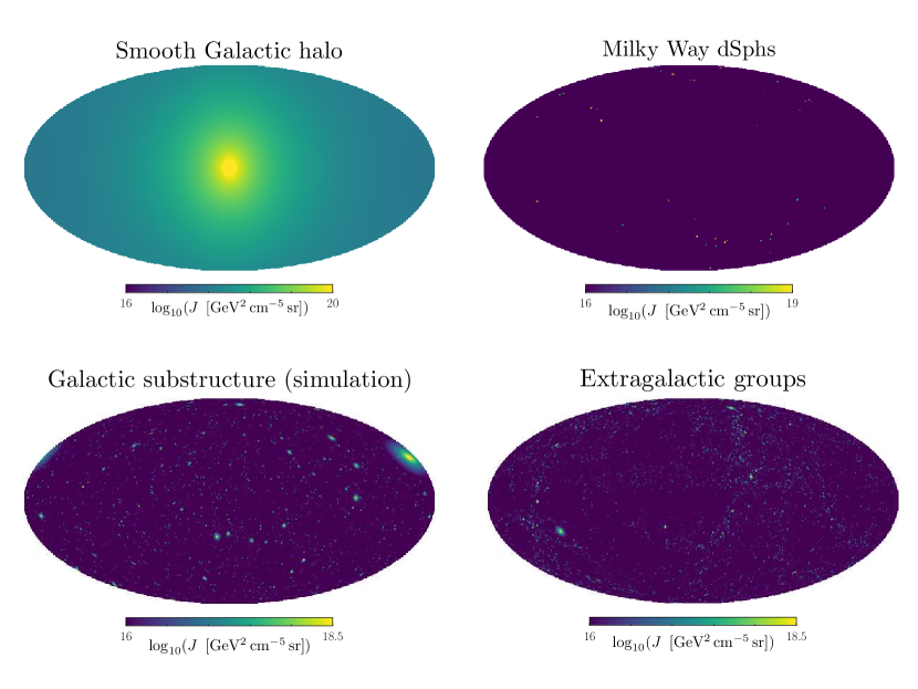
Milky Way dwarf galaxies: Dwarf spheroidal satellite galaxies (dSphs) of the Milky Way are expected to be dark matter dominated and thus to have relatively low expected astrophysical backgrounds. As such, dSphs have traditionally been considered excellent targets for DM annihilation searches. There have been about 45 dSphs candidates discovered recently by surveys like optical SDSS and DES (see Ref. [89] and references therein), and searches for gamma-ray emission from these have been able to place strong constraints on annihilation scenarios, excluding thermal WIMPs at masses below GeV at 95% confidence level for the case of annihilation into the final state [89, 90]. However, the relevant -factors are far from well-characterized—assumptions about e.g., the dSph halo shape [91, 92] and stellar membership criteria used to infer the halo properties [93, 94] can lead to significant uncertainties on the predicted annihilation signal and the corresponding annihilation limit. Figure 1.2 (top right) shows a map of the inferred -factors of dSphs considered in Ref. [89]. As in that study, the dSphs are assumed to be point-like since the shape of the corresponding DM halos is not very well constrained.
-
•
The Milky Way halo: Because of its proximity to us, the DM halo surrounding our own Galaxy is the brightest source of DM emission in the sky. Figure 1.2 (top left) shows the expected annihilation -factor for the smooth component of the Milky Way halo (see caption for further details).
Searches in the inner Galaxy (), where the signal is expected to be the brightest, have yielded an excess emission whose spatial and spectral properties can be consistent with those of a DM annihilation signal (e.g., a 40 GeV WIMP annihilating to with an approximately thermal cross section), often called the Galactic Center Excess [95, 96, 97, 98, 99, 100, 101]. This region of the sky is however plagued by the presence of substantial and difficult-to-characterize Galactic foregrounds, which complicates the interpretation of any signal and/or constraint from it. In addition, recent results based on analyzing the statistics of photons in the region [102, 103] (see also Ch. 2) indicate that the excess is more consistent with emission from an unresolved population of point sources rather than a dark matter signal, which is expected to be more diffuse in nature. There is also some evidence that the morphology of the excess emission preferentially traces the stellar overdensity in the Galactic bulge [104, 105, 106], suggesting association with an underlying stellar population.
Another class of searches focus on looking for DM emission from the Milky Way halo over larger regions of the sky at higher Galactic latitudes (), where the signal is still appreciable but Galactic foregrounds are much lower. These studies necessitate being able to accurately characterize the Galactic foreground emission over larger regions of the sky, and a careful consideration of potential foreground mismodeling effects yields stringent limits, excluding thermal WIMPs at masses below GeV at 95% confidence level for the case of annihilation into [107].
-
•
Galactic substructure: By definition, hierarchical bottom-up structure formation implies the existence of substructure (“subhalos”) within galactic DM halos, and these have the potential to be attractive DM annihilation targets. Unlike the dwarf galaxies mentioned above, low-mass subhalos with virial mass M⊙ would be mostly dark and have highly suppressed stellar activity [108, 109]. This makes it difficult to localize them and look for their gamma-ray emission. Figure 1.2 (bottom left) shows a simulated realization of -factors for Galactic substructure (subhalos) following the prescription in [110] (see caption for further details).
Traditional searches rely on assuming that the emission from unassociated gamma-ray sources detected by Fermi is coming from DM annihilation in individual subhalos, and comparing this to expectations from -body simulations [111, 112, 113, 114]. The bright source in the top right corner of the substructure map in Fig. 1.2, for example, would likely show up as a resolved unassociated source in Fermi point source catalogs such as 3FGL [115].
An orthogonal approach is to study the statistics of photons coming from DM annihilation within dim subhalos. While these subhalos may not be detectable individually, their collective emission could be detected statistically as a heightened level of “clumpiness” in the photon map. Statistical methods described in Chs. 2 and 3 of this thesis can be applied to search for such signals structure in gamma-ray data, and this approach is currently a topic of ongoing study.
-
•
Extragalactic galaxies and clusters: Searches for DM annihilation in extragalactic targets have traditionally been complicated by the difficulty in characterizing the DM properties of extragalactic halos and the presence of potentially significant astrophysical emission. Searches for emission from individual, nearby clusters [116]; the integrated, isotropic emission from background halos [117, 118, 119, 120]; and cross-correlation between gamma ray emission and catalogs of galaxies or large-scale structure [121, 122, 123, 124, 125, 126, 127, 128, 129, 130] have yielded constraints on DM annihilation properties. These searches typically do not attain sensitivity to thermal WIMPs for realistic astrophysical assumptions. Chapter 4 of this thesis focuses on developing methods to systematically characterize the dark matter emission and associated uncertainties from a large number of nearby extragalactic galaxies and clusters [131]. Figure 1.2 (bottom right) shows the extragalactic -factor map derived using this prescription and the group catalogs from Refs. [132] and [133]. Chapter 5 presents a search for gamma-ray emission using this map, which results in stringent limits on annihilating DM and excludes thermal WIMPs at masses below GeV at 95% confidence level for the case of annihilation into [134].
1.3.3 Template Methods for Gamma-Ray Searches
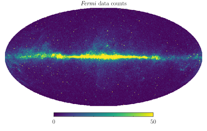
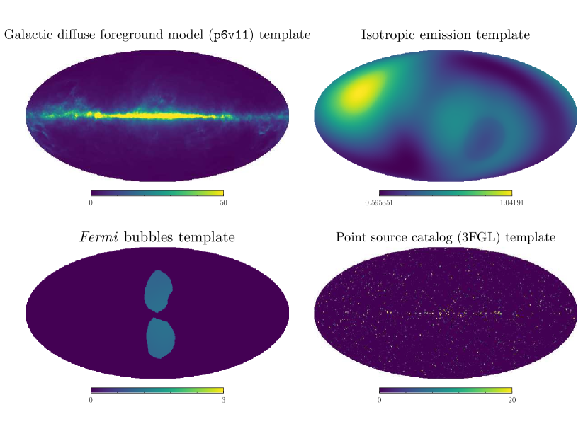
Data from gamma-ray detectors such as Fermi-LAT is typically a series of sky maps, representing the number of photons binned spatially as well as in energy. Figure 1.3 shows a subset of a typical Fermi-LAT dataset. In analyzing such data within the context of dark matter indirect detection, the challenge lies in have contributions from large-scale structures such as the smooth Galactic halo as well as point/extended sources like dwarf galaxies, from various astrophysical backgrounds. The most common technique for characterizing the various potential sources that contribute to gamma-ray data is Poissonian template fitting, which is briefly described here; a detailed description will be given in Ch. 4.
A template is a spatial map which traces the modeled contribution of a particular source or class of sources to the data, e.g. the expected emission from the diffuse Galactic foreground or resolved astrophysical point sources. Figure 1.4 shows some templates commonly used in Fermi gamma-ray analyses (see caption for descriptions). Templates for DM emission can be constructed as described in Secs. 1.3.1 and 1.3.2.
Within a single energy bin, if we denote the value of a given template in pixel by , then the total expected counts in pixel is given by
| (1.5) |
where represents the signal and background model parameters , which in this case are the normalizations of the corresponding templates. The observed data in pixel should therefore be a Poisson realization of the sum of modeled components. It follows that the likelihood function for the parameters given the data is a product over all pixels in the region-of-interest of the Poisson probabilities associated with observing counts in each pixel :
| (1.6) |
With the likelihood in hand, we can quantify the contribution of various components using conventional inference methods, e.g. obtaining posterior distributions within a Bayesian framework or building up a likelihood surfaces using frequentist profile likelihood techniques. The latter is more commonly used in DM searches—typically, we are more interested in the parameters associated with the DM model (e.g. its particle mass and annihilation cross section , which are in 1-to-1 correspondence with the normalization of the DM template) than those corresponding to the astrophysical backgrounds. A likelihood surface for the signal parameters corresponding to a given DM model can be obtained by maximizing the likelihood with respect to the background parameters at each signal parameter point. This can be generalized to the cases of analyzing several energy bins and/or stacking multiple sources (e.g. several extragalactic halos), where the total likelihood would be given by the product of the individual likelihoods.
For inferring dark matter properties, a log-likelihood difference test statistic (TS) can be defined for a given mass as
| (1.7) | ||||
where corresponds to the null signal hypothesis. Wilks’ theorem guarantees that in the asymptotic limit of a large sample size, the TS is -distributed, allowing us to discover (if we’re lucky) or exclude a DM signal in the data to a desired statistical significance in accordance with statistics. A TS value of , for example, corresponds to exclusion at a confidence level of 95%. Modified versions of this statistical procedure will be used in Chs. 4 and 5 to look for DM annihilation in extragalactic galaxies and clusters.
A fundamental limitation of Poissonian template fitting is that while resolved point sources can be either modeled with templates or masked, this is not possible for dim, sub-threshold point sources that cannot be detected individually. Depending on their spatial distribution, emission from these unresolved point sources is typically absorbed by other extended templates, e.g. isotropic (in the case of extragalactic sources) or Galactic dark matter (in the case of an approximately spherically symmetric population of unresolved sources in the Galactic center). Chapter 2 will be dedicated to extending traditional Poissonian template fitting methods to statistically account for the presence of unresolved point sources in the data.
1.4 Thesis Organization
The rest of this thesis is organized as follows. Chapter 2 describes the implementation of a novel statistical method, first introduced in Ref. [102], which leverages the “clumpiness” of photons associated with populations of unresolved point sources (PSs) in astronomical datasets to derive their contribution and properties. In Ch. 3, this method is applied to the gamma-ray sky at higher latitudes as seen by Fermi to characterize the contribution of PSs to the extragalactic gamma-ray sky over three order of magnitude in energy, from 2 to 2000 GeV. Chapter 4 poses the question “what is the best way to look for annihilating dark matter in extragalactic sources?” and attempts to answer it by constructing a pipeline to robustly map out the distribution of dark matter outside the Milky Way using galaxy group catalogs. Uncertainties involved in inferring various dark matter parameters are discussed in detail. In Ch. 5, this framework is then applied to Fermi data and existing group catalogs to search for annihilating dark matter in extragalactic galaxies and clusters.
Chapter 2 Non-Poissonian Template Fitting: Fundamentals and Code
This chapter is based on an edited version of NPTFit: A code package for Non-Poissonian Template Fitting, Astron.J. 153 (2017) no.6, 253 [arXiv:1612.03173] with Nicholas Rodd and Benjamin Safdi [142].
2.1 Introduction
Astrophysical point sources (PSs), which are defined as sources with angular extent smaller than the resolution of the detector, play an important role in virtually every analysis utilizing images of the cosmos. It is useful to distinguish between resolved and unresolved PSs; the former may be detected individually at high significance, while members of the latter population are by definition too dim to be detected individually. However, unresolved PSs—due to their potentially large number density—can be a leading and sometimes pesky source of flux across wavelengths. Recently, a novel analysis technique called the non-Poissonian template fit (NPTF) has been developed for characterizing populations of unresolved PSs at fluxes below the detection threshold for finding individually-significant sources [143, 102]. The technique expands upon the traditional fluctuation analysis technique (see, for example, [144, 145]), which analyzes the aggregate photon-count statistics of a data set to characterize the contribution from unresolved PSs, by additionally incorporating spatial information both for the distribution of unresolved PSs and for the potential sources of non-PS emission. In this work, we present a code package called NPTFit for numerically implementing the NPTF in python and cython.
The most up-to-date version of the open-source package NPTFit may be found at
https://github.com/bsafdi/NPTFit
and the latest documentation at
The NPTF generalizes traditional astrophysical template fits. Template fitting is useful for pixelated data sets consisting of some number of photon counts in each pixel , and it typically proceeds as follows. Given a set of model parameters , the mean number of predicted photon counts in the pixel may be computed. More specifically, , where is an index of the set of templates , whose normalizations and spatial morphologies may depend on the parameters . These templates may, for example, trace the gas-distribution or other extended structures that are expected to produce photon counts. Then, the probability to detect photons in the pixel is simply given by the Poisson distribution with mean . By taking a product of the probabilities over all pixels, it is straightforward to write down a likelihood function as a function of .
The NPTF modifies this procedure by allowing for non-Poissonian photon-count statistics in the individual pixels. That is, unresolved PS populations are allowed to be distributed according to spatial templates, but in the presence of unresolved PSs the photon-count statistics in individual pixels, as parameterized by , no longer follow Poisson distributions. This is heuristically because we now have to ask two questions in each pixel: first, what is the probability, given the model parameters that now also characterize the intrinsic source-count distribution of the PS population, that there are PSs within the pixel , then second, given that PS population, what is the probability to observe photons?
It is important to distinguish between resolved and unresolved PSs. Once a PS is resolved—that is once its location and flux is known—that PS may be accounted for by its own Poissonian template. Unresolved PSs are different because their locations and fluxes are not known. When we characterize unresolved PSs with the NPTF, we characterize the entire population of unresolved sources, following a given spatial distribution, based on how that population modifies the photon-count statistics.
The NPTF has played an important role recently in addressing various problems in gamma-ray astroparticle physics with data collected by the Fermi-LAT gamma-ray telescope.***http://fermi.gsfc.nasa.gov/ The NPTF was developed to address the excess of gamma rays observed by Fermi at GeV energies originating from the inner regions of the Milky Way [96, 97, 146, 147, 148, 149, 99, 150, 95, 98, 151, 100, 106, 152]. The GeV excess, as it is commonly referred to, has received a significant amount of attention due to the possibility that the excess emission arises from dark matter (DM) annihilation. However, it is well known that unresolved PSs may complicate searches for annihilating DM in the Inner Galaxy region due to, for example, the expected population of dim pulsars [150, 153, 154, 155, 156, 157, 158, 159, 160]. In [102] (see also [161]) it was shown, using the NPTF, that indeed the photon-count statistics of the data prefer a PS over a smooth DM interpretation of the GeV excess. The same conclusion was also reached by [103] using an unrelated method that analyzes the statistics of peaks in the wavelet transformation of the Fermi data.
In the case of the GeV excess, there are multiple PS populations that may contribute to the observed gamma-ray flux and complicate the search for DM annihilation. These include isotropically distributed PSs of extragalactic origin, PSs distributed along the disk of the Milky Way such as supernova remnants and pulsars, and a potential spherical population of PSs such as millisecond pulsars. Additionally, there are various identified PSs that contribute significantly to the flux as well as a variety of smooth emission mechanisms such as gas-correlated emission from pion decay and bremsstrahlung. The power of the NPTF is that these different source classes may be given separate degrees of freedom and constrained by incorporating the spatial morphology of their various contributions along with the difference in photon-count statistics between smooth emission and emission from unresolved PSs. Although the origin of the GeV excess is still not completely settled, as even if the excess arises from PSs as the NPTF suggests the source class of the PSs remains a mystery at present, the NPTF has emerged as a powerful tool for analyzing populations of dim PSs in complicated data sets with characteristic spatial morphology.
The NPTF and related techniques utilizing photon-count statistics have also been used recently to study the contribution of various source classes to the extragalactic gamma-ray background (EGB) [145, 162, 163, 164, 165].†††The complementary analysis strategy of probabilistic catalogues has also been applied to this problem [166]. In these works it was shown that unresolved blazars would predominantly show up as PS populations under the NPTF, while other source classes such as star-forming galaxies would show up predominantly as smooth emission. For example, in [165] (described in Ch. 3) it was shown using the NPTF that blazars likely account for the majority of the EGB from 2 GeV to 2 TeV. These results set strong constraints on the flux from more diffuse sources, such as star-forming galaxies, which has significant implications for, among other problems, the interpretation of the high-energy astrophysical neutrinos observed by IceCube [167, 168, 169, 170] (see, for example, [171, 172]). This is because certain sources that contribute gamma-ray flux at Fermi energies, such as star forming galaxies and various types of active galactic nuclei, may also contribute neutrino flux observable by IceCube.
Another promising application of the NPTF is to searches of annihilating dark matter from a population of subhalos in our Galaxy. Annihilation emission from Milky Way subhalos would be characterized by three distinctive features: their spatial distribution, energy spectrum, and non-Poissonian photon-count distribution. These three features taken together can be used to effectively distinguish subhalos from more standard extragalactic sources. This approach is quite different from traditional subhalo searches that look for resolved subhalo candidates in the Fermi point-source catalog [112, 113, 114]. When the spectrum of an isolated source resembles DM, it is difficult to confirm the exotic nature of the emission [173, 111]. The NPTF-based proposal relies on looking for a population of subhalos, rather than isolated objects, and is therefore less sensitive to the variations between individual sources.
The NPTF originates from the older fluctuation analysis technique, which is sometimes referred to as the analysis. This technique has been used extensively to study the flux of unresolved X-ray sources [174, 175, 176, 177, 144]. In these early works, the photon-count probability distribution function (PDF) was computed numerically for different PS source-count distributions using Monte Carlo (MC) techniques. The fluctuation analysis was first applied to gamma-ray data in [145],‡‡‡The fluctuation analysis has more recently been applied to both gamma-ray [178] and neutrino [179] datasets. and in that work the authors developed a semi-analytic technique utilizing probability generating functions for calculating the photon-count PDF. The code package NPTFit presented in this work uses this formalism for efficiently calculating the photon-count PDF. The specific form of the likelihood function for the NPTF, while reviewed in this work, was first presented in [102]. The works [102, 161, 165] utilized an early version of NPTFit to perform their numerical analyses.
The NPTFit code package has a python interface, though the likelihood evaluation is efficiently implemented in cython [180]. The user-friendly interface allows for an arbitrary number of PS and smooth templates. The PS templates are characterized by pixel-dependent source-count distributions , where is the spatial template tracking the distribution of point sources on the sky and is the pixel-independent source-count distribution. The distribution quantifies the number of sources that contributes flux between and in the pixel . The are parameterized as multiply broken power-laws, with an arbitrary number of breaks. The code is able to account for both an arbitrary exposure map (accounting for the pointing strategy of an instrument) as well as an arbitrary point spread function (PSF, accounting for the instrument’s finite angular resolution) in translating between flux (in units of photons cm-2 s-1) and photon counts .
NPTFit has a built-in interface with MultiNest [181, 182], which efficiently implements nested sampling of the posterior distribution and Bayesian evidence for the user-specified model, given the specified data and instrument response function, in the Bayesian framework [183, 184, 185]. The interface handles the Message Passing Interface (MPI), so that inference may be performed efficiently using parallel computing. A basic analysis package is provided in order to facilitate easy extraction of the most relevant data from the posterior distribution and quick plotting of the MultiNest output. The preferred format of the data for NPTFit is HEALPix [186] (a nested equal-area pixelation scheme of the sky), although the the code is also able to handle non-HEALPix data arrays. Note that the code package may also be used to simply extract the NPTF likelihood function so that NPTFit may be interfaced with any numerical package for Bayesian or frequentist inference.
A large set of example Jupyter [187] notebooks and python files are provided to illustrate the code. The examples utilize 413 weeks of processed Fermi Pass 8 data in the UltracleanVeto event class collected between August 4, 2008 and July 7, 2016 in the energy range from 2 to 20 GeV. We restrict this dataset to the top quartile as graded by PSF reconstruction in order to reduce cosmic-ray contamination and further apply the standard quality cuts DATA_QUAL==1 && LAT_CONFIG==1, as well as restricting the zenith angle to be less than . This data is made available in the code release. Moreover, the example notebooks illustrate many of the main results in [102, 161, 165].
In addition to the above, the base NPTFit code makes use of the python packages corner [188], matplotlib [189], mpmath [190], GSL [191] and numpy [192].
The rest of this chapter is organized as follows. Section 2.2 outlines in more detail the framework of the NPTF. Sections 2.3 and 2.4 describe further details behind the mathematical framework of the NPTF. Section 2.5 highlights the key classes and features in the NPTFit code package and usage instructions. In Sec. 2.6 we present an example of how to perform an NPTF scan using NPTFit, looking at the Galactic Center with Fermi data to reproduce aspects of the main results of [102]. We conclude in Sec. 2.7.
2.2 The Non-Poissonian Template Fit
In this section we review the NPTF, which was first presented in [102] and described in more detail in [161, 165] (see also [145, 143, 162, 164] and Ch. 3). The NPTF is used to fit a model with parameters to a data set consisting of counts (i.e., number of photon) in each pixel . The likelihood function for the NPTF is then simply
| (2.1) |
where gives the probability of drawing counts in the given pixel , as a function of the parameters . The main computational challenge, of course, is in computing these probabilities.
It is useful to divide the model parameters into two different categories: the first category describes smooth templates, while the second category describes PS templates. We describe each category in turn, starting with the smooth templates.
For most applications, the data has the interpretation of being a two-dimensional pixelated map consisting of an integer number of counts in each pixel. The smooth templates may be used to predict the mean number of counts in each pixel :
| (2.2) |
Above, is an index over templates and denotes the mean contribution of the template to pixel for parameters . In principle, may describe both the spatial morphology as well as the normalization of the templates. However, in the current implementation of the code, the Poissonian model parameters simply characterize the overall normalization of the templates: . Here, is the normalization parameter and is the template, which takes values over all pixels and is independent of the model parameters. The superscript implies that the template is a counts templates, which is to be contrasted with a flux template, for which we use the symbol . The two are related by the exposure map of the instrument : . In the case where we only have smooth, Poissonian templates, the probabilities are then given by the Poisson distribution:
| (2.3) |
In the presence of unresolved PS templates, the probabilities are no longer Poissonian functions of the model parameters . Each PS template is characterized by a pixel-dependent source-count distribution , which describes the differential number of sources per pixel per unit flux interval. In this work, we model the source-count distribution by a multiply broken power-law:
| (2.4) |
Above, we have parameterized the source-count distribution with an arbitrary number of breaks , denoted by with , and indices with . The spatial dependence of the source-count distribution is accounted for by the overall factor , where is the pixel-independent normalization, which is a function of the model parameters, and is a template describing the spatial distribution of the PSs. More precisely, the number of sources (and the total PS flux ) in pixel , for a fixed set of model parameters , follows the template . On the other hand, the locations of the flux breaks and the indices are taken to be fixed between pixels.§§§In principle, the breaks and indices could also vary between pixels. However, in the current version of NPTFit, only the number of sources (and, accordingly, the total flux) is allowed to vary between pixels.
To summarize, a PS template described by a broken power-law with breaks has model parameters describing the locations of the breaks, the power-law indices, and the overall normalization. For example, if we take a single break then the PS model parameters may be denoted as . Additionally, a spatial template must be specified, which describes the distribution of the number of sources (and total flux) with pixel .
Notice that when we discussed the Poissonian templates we used the counts templates and talked directly in terms of counts , while so far in our discussion of the unresolved PS templates we have used the point source distribution template and written the source-count distribution in terms of flux . Of course as the total flux from a distribution of point sources is also proportional to the template , it can be thought of as a flux template, however conceptually it is being used to track the distribution of the sources rather than the flux they produce. For this reason we have chosen to distinguish the two. Moreover, in the presence of a non-trivial PSF, should also be smoothed by the PSF to account for the instrument response function. That is, is a template for the observed counts taking into account the details of the instrument, while () is a map of the physical point sources (flux), which is independent of the instrument. In photon-counting applications, the exposure map often has units of and flux has units of .
For the unresolved PS templates, we also need to convert the source-count distribution from flux to counts. This is done by a simple change of variables:
| (2.5) |
which implies that for a non-Poissonian template the spatial dependence of is given by . This inverse exposure scaling may seem surprising, but it is straightforward to confirm that the mean number of counts in a given pixel, , is given by , as expected, up to pixel independent factors.
As an important aside, the template used by the Poissonian models needs to be smoothed by the PSF. Incorporating the PSF into the unresolved PS models, on the other hand, is more complicated and is not accomplished simply by smoothing the spatial template. Indeed, should remain un-smoothed by the PSF when used for non-Poissonian scans. Accounting for PSF effects in the non-Poissonian likelihood will be described in detail in Sec. 2.3.2.
In the remainder of this section we briefly overview the mathematic framework behind the computation of the with NPTFit; however, details of the algorithms used to calculate these probabilities in practice, along with more in-depth explanations, are given in Secs. 2.3 and 2.4. We use the probability generating function formalism, following [145], to calculate the probabilities. For a discrete probability distribution , with , the generating function is defined as:
| (2.6) |
from which we can recover the probabilities:
| (2.7) |
The key feature of generating functions exploited here is that the generating function of a sum of two independent random variables is simply the product of the individual generating functions.
The probability generating function for the smooth templates, as a function of , is simply given by
| (2.8) |
The probability generating function for an unresolved PS template, on the other hand, takes a more complicated form (derived in Sec. 2.3):
| (2.9) |
where
| (2.10) |
Above, is a function that takes into account the PSF, which we describe in more detail in Sec. 2.3. In the presence of a non-trivial PSF, the flux from a single source is smeared among pixels. The distribution of flux fractions among pixels is described by the function , where is the flux fraction. By definition equals the number of pixels which, on average, contain between and of the flux from a PS; the distribution is normalized such that . If the PSF is a -function, then .
Putting aside the PSF correction for the moment, the have the interpretation of being the average number of -count PSs within the pixel , given the distribution . The generating function for -count sources is simply (see [145] or Sec. 2.3), which then leads directly to (2.9). The PSF correction, through the distribution , incorporates the fact that PSs only contribute some fraction of their flux within a given pixel.
2.3 Mathematical Foundations of NPTFit
In this section we present the mathematical foundation of the NPTF and the evaluation of the non-Poissonian likelihood in more detail that what was shown in Sec. 2.2. Note that many of the details presented in this section have appeared in the earlier works of [145, 143, 102], however we have reproduced these here in order to have a single clear picture of the method.
The remainder of this section is divided as follows. Firstly we outline how to determine the generating functions for the Poissonian and non-Poissonian case. We then describe how we account for finite PSF corrections.
2.3.1 The (non-)Poissonian Generating Function
There are two reasons why the evaluation of the Poissonian likelihood for traditional template fitting can be evaluated rapidly. The first of these is that the functional form of the Poissonian likelihood is simple. Secondly, and more importantly, is the fact that if we have two discrete random variables and that follow Poisson distributions with means and , then the random variable again follows a Poisson distribution with mean . This generalizes to combining an arbitrary number of random Poisson distributed variables and is why we were able to write in Sec. 2.2. This fact is not true when combining arbitrary random variables, and in particular if we add in a template following non-Poissonian statistics.
An elegant solution to this problem was introduced in [145], using the method of generating functions. As we are always dealing with pixelized maps containing discrete counts (of photons or otherwise), for any model of interest there will always be a discrete probability distribution , the probability of observing counts. In terms of these, we then define the probability generating function as in (2.6). The property of probability generating functions that make them so useful in the present context is as follows. Consider two random processes and , with generating functions and , that follow arbitrary and potentially different statistical distributions. Then the generating function of is simply given by the product . In this subsection we will derive the appropriate form of for Poissonian and non-Poissonian statistics.
To begin with, consider the purely Poissonian case. Here and throughout this section we consider only the likelihood in a single pixel; the likelihood over a full map is obtained from the product of the pixel-based likelihoods. Then for a Poisson distribution with an expected number of counts in a pixel :
| (2.11) |
Note that the variation of the across the full map will be a function of the model parameters, such that . In order to simplify the notation in this section however, we leave the dependence implicit. Given the values, we then have:
| (2.12) | ||||
From this form, it is clear that if we have two Poisson distributions with means and , the product of their generating functions will again describe a Poisson distribution, but with mean .
Next we work towards the generating function in the non-Poissonian case. At the outset, we let denote the average number of sources in a pixel that emit exactly counts. In terms of this, the probability of finding -count sources in this pixel is just a draw from a Poisson distribution with mean , i.e.
| (2.13) |
Given this, the probability to find counts from a population of -count sources is
| (2.14) |
We can then use this to derive the non-Poissonian -count generating function as follows:
| (2.15) | ||||
However this is just the generating function for -count sources, to get the full non-Poissonian generating function we need to multiply this over all values of . Doing so we arrive at
| (2.16) | ||||
justifying the form given in Sec. 2.2. Again recall for the full likelihood we can just multiply the pixel based likelihoods and that .
So far we have said nothing of how to determine , the average number of -count source in pixel . This value depends on the source-count distribution , which specifies the distribution of sources as a function of their expected number of counts, . Of course the physical object is , where is the flux. This distinction was discussed in Sec. 2.2, and can be implemented in NPTFit to arbitrary precision. Nevertheless does not fully determine —we need to account for the fact that a source that is expected to give photons could Poisson fluctuate to give . As such any source can in principle contribute to , and so integrating over the full distribution we arrive at:
| (2.17) |
An important part of implementing the NPTF in a rapid manner, which is a central feature of NPTFit, is the analytic evaluation of the integral in this equation. In order to do this, we need to have a specific form of the source-count distribution. For this purpose, we allow the source count distribution to be a multiply broken power-law and evaluate the integral for any number of breaks.
Putting the evaluation of the integral aside for the moment then, we have arrived at the full non-Poissonian generating function:
| (2.18) | ||||
Contrasting this with Eq. (2.12), we see that whilst the Poissonian likelihood is specified by a single number , the non-Poissonian likelihood is instead specified by a distribution .
In the case of multiple PS templates, we should multiply the independent probability generating functions. However, this is equivalent to summing the parameters. This is how multiple PS templates are incorporated into the NPTFit code:
| (2.19) |
where the sum over is over the contributions from individual PS templates.
2.3.2 Correcting For a Finite Point Spread Function
The next factor to account for is the fact that in any realistic dataset there will be a non-zero PSF. Here, we closely follow the discussion in [145]. The PSF arises due to the inability of an instrument to perfectly reconstruct the original direction of the photon, neutrino, or quantity making up the counts. In practice, a finite PSF means that a source in one pixel can contribute counts to nearby pixels as well. To implement this correction, we modify the calculation of given in Eq. (2.18), which accounts for the distribution of sources as a function of and the fact that each one could Poisson fluctuate to give us counts. The finite PSF means that in addition to this, we also need to draw from the distribution , that determines the probability that a given source contributes a fraction of its flux in a given pixel. Once we know , this modifies our calculation of in Eq. (2.18)—now a source that is expected to contribute counts, will instead contribute , where is drawn from . As such we arrive at the result in (2.10).
In NPTFit we determine using Monte Carlo. To do this we place a number of PSs appropriately smeared by the PSF at random positions on a pixelized sphere. Then integrating over all pixels we can determine the fraction of the flux in each pixel , , defined such that . Note in practice one can truncate this sum at some minimal value of without impacting the argument below. From the set , we then denote by the number of fractions for point sources that fall within some range . From these quantities, we may determine as
| (2.20) |
which is normalized such that . From this definition we see that the case of a vanishing PSF is just - i.e. the flux is always completely in the pixel with the PS.
2.4 NPTFit: Algorithms
The generating-function formalism for calculating the probabilities is described at the end of Sec. 2.2 and in more detail in Sec. 2.3. In particular—given the generating function —we are instructed to calculate the probabilities by taking derivatives as in (2.7). However, taking derivatives is numerically costly, and so instead we have developed recursive algorithms for computing these probabilities. In the same spirit, we analytically evaluate the parameters defined in (2.10) for the multiply-broken source-count distribution in order to facilitate a fast evaluation of the NPTF likelihood function. In this section, we overview these methods that are essential to making NPTFit a practical software package.
In general we may write the full single pixel generating function for a model containing an arbitrary number of Poissonian and non-Poissonian templates as:
| (2.21) |
where we have defined
| (2.22) |
Above, represents the average number of -count source in pixel . The remaining task is to efficiently calculate the probabilities , which are formally defined in terms of derivatives through (2.7). Nevertheless, derivatives are slow to implement numerically, so we instead use a recursion relation to determine in terms of .
To begin with, note that
| (2.23) |
For the rest of this discussion, we suppress the pixel index , though one should keep in mind that this process must be performed independently in every pixel. From (2.23), we can immediately write down
| (2.24) | ||||
Given and , we may write our recursion relation for as
| (2.25) |
which as mentioned requires the knowledge of all . To derive (2.25), we first define
| (2.26) |
Then, for example,
| (2.27) |
From here to determine we simply need more derivatives. Using the generalized Leibniz rule, we have
| (2.28) | ||||
Then setting and recalling the definition of , this yields
| (2.29) | ||||
as claimed.
To calculate the in a pixel , we need to calculate the and the sum . We may calculate these expressions analytically using the general source-count distribution in (2.4). To calculate the sums, we make use of the relation
| (2.30) | ||||
Finiteness of the total flux, and also the probabilities, requires and . However, both the integral and , appearing in the last line above, may be divergent individually if . In this case, we analytically continue in , evaluate the contributions individually, and then sum the two expressions to get a result that is finite across the whole range of allowable parameter space.
2.5 NPTFit: Orientation
NPTFit implements the NPTF, as described above, in python. In this section we give a brief orientation to the code package and its main classes. A more thorough description of the code and its uses is available in the online documentation.
class NPTFit.nptfit.NPTF
This is the main class used to set up and perform non-Poissonian and Poissonian template scans. It is initialized by
with keywords
| Argument | Default | Purpose | type |
| tag | ’Untagged’ | Label of scan | str |
| work_dir | None | Output directory | str |
.
If no work_dir is specified, the code will default to the current directory. This is the directory where all output is stored. Specifying a tag will create an additional folder, with that name, within the work_dir for the output.
The data, exposure map, and templates are loaded into the nptfit.NPTF instance after initialization (see the example in Sec. 2.6). The data and exposure map are loaded by
Here, data and exposure are 1-D numpy arrays. The recommended format for these arrays is the HEALPix format, so that all pixels are equal area, although the code is able to handle arbitrary data and exposure arrays so long as they are of the same length. The templates are added by
Here, template is a 1-D numpy array of the same length as the data and exposure map, key is a string that will be used to refer to the template later on, and units specifies whether the template is a counts template (keyword ’counts’) or a flux template (keyword ’flux’) in units . The default, if unspecified, is units = ’counts’. The template should be pre-smoothed by the PSF if it is going to be used for a Poissonian model. If the template is going to be used for a non-Poissonian model, either choice for units is acceptable, though in the case of ’counts’ the template should simply be the product of the exposure map times the flux template and not smoothed by the PSF.
The user also has the option of loading in a mask that reduces the region of interest (ROI) to a subset of the pixels in the data, exposure, and template arrays. This is done through the command
where mask is a boolean numpy array of the same length as the data and exposure arrays. Pixels in mask should be either True or False; by convention, pixels that are True will be masked, while those that are False will not be masked. Note if performing an analysis with non-Poissonian templates, regions where the exposure map is identically zero should be explicitly masked.
Afterwards, Poissonian and non-Poissonian models may be added to the instance using the available templates. An arbitrary number of Poissonian and non-Poissonian models may be added to the scan. Moreover, each non-Poissonian model may be specified in terms of a multiply broken power law with a user-specified number of breaks, as in (2.4).
Poissonian models are added sequentially using the syntax
where the keywords are
| Argument | Default | Purpose | type |
| template_name | - | key of template | str |
| model_tag | - | LaTeX-ready label | str |
| prior_range | [] | Prior [min, max ] | [float, float] |
| log_prior | False | Log/linear-flat prior | bool |
| fixed | False | Is template fixed | bool |
| fixed_norm | 1.0 | Norm if fixed | float |
Any of the model parameters may be fixed to a user specified value instead of floated in the scan. For those parameters that are floated in the scan, a prior range needs to be specified along with whether or not the prior is flat or log-flat. Note that if log_prior = True, then the prior range is set with respect to of the linear prior range.¶¶¶More complicated priors will be incorporated in future releases of NPTFit. For example, if we want to scan the normalization of a template over the range from with a log-flat prior, then we would set log_prior = True and prior_range = [-1,1]. In this case, it might make sense to label the model with model_tag = ’$\log_{10}A$’ to emphasize that the actual model parameter is the log of the normalization; this label will appear in various plots made using the provided analysis class for visualizing the posterior.
The non-Poissonian models are added with a similar syntax:
The template_name keyword is the same as for the Poissonian models. The rest of the keywords are
| Argument | Default | Purpose | type |
| model_tag | - | LaTeX-ready label | [str, str, ...] |
| prior_range | [] | Prior [[min, max], …] | [[float, float], ...] |
| log_prior | [False] | Log/linear-flat prior | [bool,bool, ...] |
| dnds_model | ’specify_breaks’ | How to specify multiple breaks | str |
| fixed_params | None | Fix certain parameters | [[int,float], ...] |
| units | ’counts’ | ’flux’ or ’counts’ units for breaks | str |
The syntax for adding non-Poissonian models is that the model parameters are specified by for a broken power-law with breaks. As such, the model_tag, prior_range, and log_prior are now arrays where each entry refers to the respective model parameter. The code automatically determines the number of breaks by the length of the model_tag array. The arrays prior_range and log_prior should only include entries for model parameters that will be floated in the scan. Any model parameter may be fixed using the fixed_params array, with the syntax such that fixed_params = [[i,c_i],[j,c_j]] would fix the model parameter to and the to , where the parameter indexing starts from 0.
The units keyword determines whether the priors for the breaks in the source-count distribution (and also the fixed parameters, if any are given) will be specified in terms of ’flux’ or ’counts’. The relation between flux and counts varies between pixels if the exposure map is non-trivial. For this reason, it is more appropriate to think of the breaks in the source-count distribution in terms of flux. The keyword ’counts’ still specifies the breaks in the source-count distribution in terms of flux, with the relation between counts and flux given through the mean of the exposure map : .
The dnds_model keyword has the options ’specify_breaks’ and ’specify_relative_breaks’. If ’specify_breaks’ is chosen, which is the default, then the breaks are the model parameters. If instead ’specify_relative_breaks’ is chosen, the full set of model parameters is given by . Here, is the highest break and the lower breaks are determined by . Note that the prior ranges for the ’s should be between and (for linear flat), since .
After setting up a scan, the configuration is finished by executing the command
For a purely Poissonian scan, none of the keywords above need to be specified. For non-Poissonian scans, f_ary and df_rho_div_f_ary incorporate the PSF correction. In particular, f_ary is a discretized list of values between and , while df_rho_div_f_ary is a discretized list of at those values. A class is provided for computing these lists; it is described later in this section. If no keywords are given for these two arrays they default to the case of a -function PSF.
The keyword nexp, which defaults to , is related to the exposure correction in the calculation of the source-count distribution from . In many applications, it is computationally too expensive to perform the mapping in (2.5) in each pixel. The overall pixel-dependent normalization factor factorizes from many of the internal computations, and as a result this contribution to the exposure correction is performed in every pixel. However, it is useful to perform the mapping from flux to counts, which should be performed uniquely in each pixel , using the mean exposure within small sub-regions. Within a given sub-region, we map flux to counts using , where the mean is taken over all pixels in the sub-region. The number of sub-regions is given by nexp, and all sub-regions have approximately the same area. As nexp approaches the number of pixels, the approximation becomes exact; however, for many applications the approximation converges for a relatively small number of exposure regions. We recommend verifying, in any application, that results are stable as nexp is increased.
After configuring the NPTF instance, the log-likelihood may be extracted, as a function of the model parameters, in addition to the prior range. The log-likelihood and prior range may then be used with any external package for performing Bayesian or frequentist inference. This is particularly useful if the user would like to combine likelihood functions between different energy bins or otherwise add to the default likelihood function, for example, incorporating nuisance parameters beyond those associated with individual templates. The package MultiNest, however, is already incorporated into the NPTF class and may be run immediately after configuring the NPTF instance. This is done simply by executing the command
where nlive is an integer that specifies the number of live points used in the sampling of the posterior distribution. MultiNest recommends an nlive 500-1000, though the parameter defaults to if unspecified for quick test runs. Additional MultiNest arguments may be passed as a dictionary through the optional pymultinest_options keyword (see the online documentation for more details). The optional keyword run_tag is used to create a sub-folder for the MultiNest output with that name.
After a scan has been run (or if a scan has been run previously and saved), the results may be loaded through the command
The MultiNest chains, which give a discretized view of the posterior distribution, may then be accessed through, for example, nptf.samples. An instance of the PyMultiNest analyzer class may be accessed through nptf.a. A small analysis package, described later in this section, is also provided for performing a few common analyses.
class NPTFit.psf_correction.PSFCorrection
This is the class used to construct the arrays f_ary and df_rho_div_f_ary for the PSF correction. An instance of PSFCorrection is initialized through
with keywords
| Argument | Default | Purpose | type |
| psf_dir | None | Where PSF arrays are stored | str |
| num_f_bins | 10 | Number of linear-spaced points inf_ary | int |
| n_psf | 50000 | Number of MC simulations for determining df_rho_div_f_ary | int |
| n_pts_per_psf | 1000 | Number of points drawn for each MC simulation | int |
| f_trunc | 0.01 | Minimum value | float |
| nside | 128 | HEALPix parameter for size of map | int |
| psf_sigma_deg | None | Standard deviation of 2-D Gaussian PSF | float |
| delay_compute | False | If True, PSF not Gaussian and will be specified later | bool |
Note that the arrays f_ary and df_rho_div_f_ary depend both on the PSF of the detector as well as the pixelation of the data; at present the PSFCorrection class requires the pixelation to be in the HEALPix pixelation.
The keyword psf_dir points to the directory where the f_ary and df_rho_div_f_ary will be stored; if unspecified, they will be stored to the current directory. The f_ary consists of num_f_bins entries linear spaced between and . The PSF correction involves placing many (n_psf) PSFs at random positions on the HEALPix map, drawing n_pts_per_psf points from each PSF, and then looking at the distribution of points among pixels. The larger n_psf and n_pts_per_psf, the more accurate the computation of df_rho_div_f_ary will be. However, the computation time of the PSF arrays also increases as these parameters are increased.
By default the PSFCorrection class assumes that the PSF is a 2-D Gaussian distribution:
| (2.31) |
Here, describes the spread of arriving counts with angular distance away from the arrival direction. The parameter psf_sigma_deg denotes in degrees. Upon initializing PSFCorrection with psf_sigma_deg specified, the class automatically computes the array df_rho_div_f_ary and stores it in the psf_dir with a unique name related to the keywords. If such a file already exists in the psf_dir, then the code will simply load this file instead of recomputing it. After initialization, the relevant arrays may be accessed by pc_inst.f_ary and pc_inst.df_rho_div_f_ary.
The PSFCorrection class can also handle arbitrary PSF functions. In this case, the class should be initialized with delay_compute = True. Then, the user should manually set the function pc_inst.psf_r_func to the desired function . This function will be discretized with pc_inst.psf_samples points out to pc_inst.sample_psf_max degrees from . These two quantities also need to be manually specified. The user also needs to set pc_inst.psf_tag to a string that will be used for saving the PSF arrays. After these four attributes have been set manually by the user, the PSF arrays are computed and stored by executing pc_inst.make_or_load_psf_corr().
def NPTFit.create_mask.make_mask_total
This function is used to make masks that can then be used to reduce the data and templates to a smaller ROI when performing the scan. While these masks can always be made by hand, this function provides a simple masking interface for maps in the HEALPix format. The make_mask_total function can mask pixels by latitude, longitude, and radius from any point on the sphere. See the online documentation for more specific examples.
class NPTFit.dnds_analysis.Analysis
The analysis class may be used to extract useful information from the results of an NPTF performed using MultiNest. The class also has built-in plotting features for making many of the most common types of visualizations for the parameter posterior distribution. An instance of the analysis class can be instantiated by
where nptf is itself an instance of the NPTF class that already has the results of a scan loaded. The keyword arguments mask and pixarea are optional. The user should specify a mask if the desired ROI for the analysis is different that that used in the scan. The user should specify a pixarea if the data is not in the HEALPix format. The code will still assume the pixels are equal area with area pixarea, which should be specified in sr.
After initialization, the intensities of Poissonian and non-Poissonian templates, respectively, may be extracted from the analysis class by the commands
and
Here, comp refers to the template key used by the Poissonian or non-Poissonian model. The arrays returned give the mean intensities of that model in the ROI in units of , assuming the exposure map was in units of cm2s. The arrays computed over the full set of entries in the discretized posterior distribution output by MultiNest. Thus, these intensity arrays may be interpreted as the 1-D posteriors for the intensities. For additional keywords that may be used to customize the computation of the intensity arrays, see the online documentation.
The source-count distributions may also be accessed from the analysis class. Executing
will return the discretized 1-D posterior distribution for at flux for the PS model with template key comp. Note that the mean is computed over pixels in the ROI.
The 1-D posterior distributions for the individual model parameters may be accessed by
for Poissonian models, and
for non-Poissonian models. Here A_poiss_post is a 1-D array of the discretized posterior distribution for the Poissonian template normalization parameter. Similarly, A_non_poiss_post is the posterior array for the non-Poissonian normalization parameter. The arrays n_non_poiss_post and Sb_non_poiss_post are 2-D, where—for example—n_non_poiss_post = [n_1_array, n_2_array, ...] and n_1_array is a 1-D array for the posterior for .
Another useful piece of information that may be extracted from the scan is the Bayesian evidence:
returns the log of the Bayesian evidence along with the uncertainty on this estimate based on the resolution of the MCMC.
For information on the plotting capabilities in the analysis class, see the online documentation or the example in the following section.
2.6 NPTFit: An Example
In this section we give an example for how to perform an NPTF using NPTFit. Many more examples are available in the online documentation. This particular example reproduces aspects of the main results of [102], which found evidence for a spherical population of unresolved gamma-ray PSs around the Galactic Center. The example uses the processed, public Fermi data made available with the release of the NPTFit package. The data set consists of 413 weeks of Fermi Pass 8 data in the UltracleanVeto event class (top quartile of events as ranked by PSF) from 2 to 20 GeV. The map is binned in HEALPix with . The data, along with the exposure map and background templates, may be downloaded from
In the example we will perform an NPTF on the sub-region where we mask the Galactic plane at latitude and mask pixels with angular distance greater than from the Galactic Center. We also mask identified PSs in the 3FGL PS catalog [115] at 95% containment using the provided PS mask, which is added to the geometric mask. We include smooth templates for diffuse gamma-ray emission in the Milky Way (using the Fermi p6v11 diffuse model), isotropic emission (which can also absorb instrumental backgrounds), and emission following the Fermi bubbles, which are taken to be uniform in flux following the spatial template in [140]. We also include a dark matter template, which traces the line of sight integral of the square of a canonical NFW density profile.
We additionally include point source (non-Poissonian) models for the DM template, as well as for a disk template which corresponds to a doubly exponential thin-disk source distribution with scale height 0.3 kpc and radius 5 kpc. The source-count distributions for these are parameterized by singly-broken power laws, each described by four parameters .
2.6.1 Setting Up the Scan
We begin the example by loading in the relevant modules, described in the previous section, that we will need to setup, perform, and analyze the scan.
Next, we create an instance of the NPTF class, which is used to configure and perform a scan.
We assume here that the supplementary Fermi data has been downloaded to a directory ’fermi_data’. Then, we may load in the data and exposure maps by
Importantly, note that the exposure map has units of cm2s. Next, we use the create_mask class to generate our ROI mask, which consists of both the geometric mask and the PS mask loaded in from the ’fermi_data’ directory:
The templates may also be loaded in from this directory,
These templates are counts map (i.e. flux maps times the exposure map) that have been pre-smoothed by the PSF (except for the disk-correlated template labeled dsk). We then add them to our NPTF instance with appropriately chosen keywords:
Note that templates ’gce_np’ and ’dsk_np’ intended to be used in non-Poissonian models should trace the underlying PS distribution, without exposure correction, and are added with the keyword units=’PS’.
2.6.2 Adding Models
Now that we have loaded in all of the external data and templates, we can add models to our NPTF instance. First, we add in the Poissonian models,
All Poissonian models are taken to have linear priors, with prior ranges for the normalizations between 0 and 2. However, the normalization of the diffuse background has been fixed to the value , which is approximately the correct normalization in these units for this template, in order to provide an example of this syntax. Next, we add in the two non-Poissonian models:
We have added in the models for disk-correlated and NFW-correlated (line of sight integral of the the NFW distribution squared) unresolved PS templates. Each of these models takes singly-broken power-law source-count distributions. In this configuration, the normalization parameters are taken to have a log-flat prior while the indices and breaks are taken to have linear priors (relevant for the Bayesian posterior sampling). The units of the breaks are specified in terms of counts.
2.6.3 Configure Scan with PSF Correction
In this energy range and with this data set, the PSF may be modeled by a 2-D Gaussian distribution with . From this, we are able to construct the PSF-correction arrays:∥∥∥For an example of how to construct these arrays with a more complicated, non-Gaussian PSF function, see the online documentation.
These arrays are then passed into the NPTF instance when we configure the scan:
Note that since our ROI is relatively small and the exposure map does not change significantly over the region, we have a single exposure region with nexp=1.
2.6.4 Performing the Scan With MultiNest
We perform the scan using MultiNest with nlive=500 as an example to demonstrate the basic features and conclusions of this analysis while being able to perform the scan in a reasonable amount of time on a single processor, although ideally nlive should be set to a higher value for more reliable results:
2.6.5 Analyzing the Results
Now, we are ready to analyze the results of the scan. First we load in relevant modules:
and then we load in the results of the scan (configured as above),
The chains, giving a discretized view of the posterior distribution, may be accessed simply through the attribute n.samples. However, we will analyze the results by using the analysis class provided with NPTFit. We make an instance of this class simply by
Making Corner Plots
Corner (or triangle) plots are a simple and quick way of visualizing correlations in the posterior distribution. Such plots may be generated through the command
which leads to the plot in Fig. 2.1.
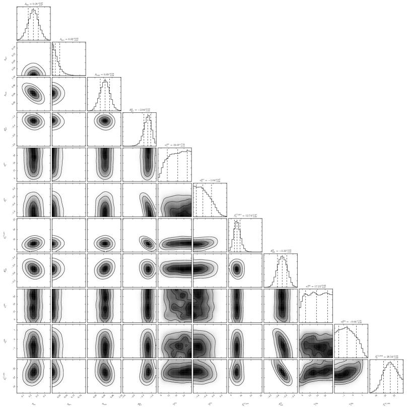
Plotting Source-count Distributions
The source-count distributions for NFW- and disk-correlated point source models may be plotted with
along with the following matplotlib plotting options.
This is shown in Fig. 2.2. Contribution from both NFW- and disk-correlated PSs may be seen, with NFW-correlated sources contributing dominantly at lower flux values. In that figure, we also show a histogram of the detected 3FGL sources within the relevant energy range and region, with vertical error bars indicating the 68% confidence interval from Poisson counting uncertainties only.******The data for plotting these points is available in the online documentation. Since we have explicitly masked all 3FGL sources, we see that the disk- and NFW-correlated PS templates contribute at fluxes near and below the 3FGL PS detection threshold, which is counts cm-2 s-1 in this case.
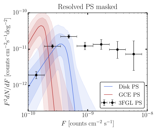
Plotting Intensity Fractions
The intensity fractions for the smooth and PS NFW-correlated models may be plotted with
This is shown in Fig. 2.3. We immediately see a preference for NFW-correlated point sources over the smooth NFW component.
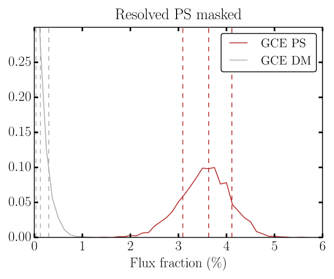
Further Analyses
The example above may easily be pushed further in many directions, many of which are outlined in [102]. For example, a natural method for performing model comparison in the Bayesian framework is to compute the Bayes factor between two models. Here, for example, we may compute the Bayes factor between the model with and without NFW-correlated PSs. This involves repeating the scan described above but only adding in disk-correlated PSs. Then, by comparing the global Bayesian evidence between the two scans (see Sec. 2.5 for the syntax on how to extract the Bayesian evidence), we find a Bayes factor in preference for the model with spherical PSs.
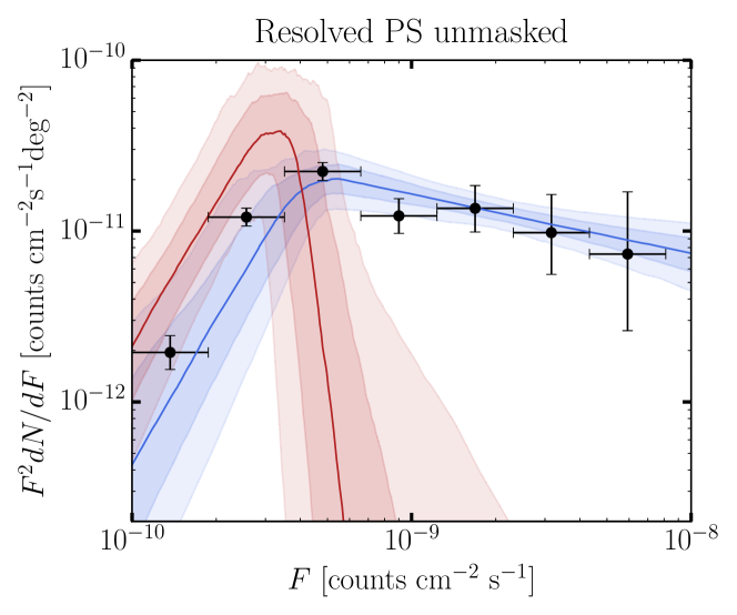
Another straightforward generalization of the example described above is simply to leave out the PS mask, so that the NFW- and disk-correlated PS templates must account for both the resolved and unresolved PSs. The likelihood evaluations take longer, in this case, since there are pixels with higher photon counts compared to the 3FGL-masked scan. The result for the source-count distribution from this analysis is shown in Fig. 2.4. In this case, the disk-correlated PS template accounts for the resolved 3FGL sources, while the NFW-correlated PS template contributes at roughly the same flux range as in the 3FGL masked case. The Bayes factor in preference for the model with NFW-correlated PSs over that without—as described above—is found to be in this case.
2.7 Conclusion
We have presented an open-source code package for performing non-Poissonian template fits. We strongly recommend referring to the online documentation—which will be kept up-to-date—in addition to this chapter accompanying the initial release. There are many way in which NPTFit can be improved in the future. For one, the NPTFit package only handles a single energy bin at a time. In a later version of the code we plan to incorporate the ability to scan over multiple energy bins simultaneously. Additionally, there are a few areas—such as the evaluation of the incomplete gamma functions—where the cython code may still be sped up. Such improvements to the computational cost are relevant for analyses of large data sets with many model parameters. Of course, we welcome additional suggestions for how we may improve the code and better adapt it to applications beyond the gamma-ray applications it has been used for so far.
Chapter 3 Application of Non-Poissonian Template Fitting to the Extragalactic Gamma-Ray Background
This chapter is based on an edited version of Deciphering Contributions to the Extragalactic Gamma-Ray Background from 2 GeV to 2 TeV, Astrophys.J. 832 (2016) no.2, 117 [arXiv:1606.04101] with Mariangela Lisanti, Lina Necib and Benjamin Safdi [165]. The results of this chapter have been presented at the following conferences and workshops: Gamma Rays and Dark Matter in Obergurgl, Austria (December 2015), TeV Particle Astrophysics (TeVPA) 2016 in Geneva, Switzerland (September 2016) and APS April Meeting 2017 in Washington, DC (January 2017).
3.1 Introduction
The Extragalactic Gamma-Ray Background (EGB) is the nearly isotropic all-sky emission that arises from sources outside of the Milky Way. The OSO-3 [193, 194] and SAS-2 satellites [195, 196] were the first to see hints of the EGB and have since been followed by EGRET [197, 198] and, most recently, the Fermi Large Area Telescope***http://fermi.gsfc.nasa.gov/ [199, 163]. The origin of the EGB remains an open question. The dominant contributions are likely due to blazars [200, 201, 202, 203, 204, 205, 206, 207, 208, 209, 210, 211, 212, 213, 118, 214], star-forming galaxies (SFGs) [215, 216, 217, 218, 219, 220, 221, 222, 223, 224], and misaligned active galactic nuclei (mAGN) [225, 226, 227, 228, 229]. Understanding the relative contributions of these source components to the EGB has taken on a new sense of importance in light of IceCube’s observation of ultra-high-energy extragalactic neutrinos [167, 168, 169, 170], the origin of which still remains a mystery. For instance, the same sources that dominate the extragalactic neutrino background at PeV energies may also contribute significantly to the EGB from GeV–TeV energies [230, 224, 229]. In addition, the EGB may harbor the imprints of more exotic physics such as dark matter annihilation or decay [231, 232, 233, 234, 43, 235, 118, 120, 117], as well as contributions from truly diffuse processes such as propagating ultra-high-energy cosmic rays [236, 237, 238, 239, 240] and structure formation shocks in clusters of galaxies [241, 242]. Given the potential wealth of information that can be extracted from the EGB, deciphering its constituents remains a high priority.
Most recently, Fermi presented a measurement of the EGB intensity from 100 MeV to 820 GeV [199]. The total EGB intensity is the sum of all resolved point sources (PSs) and smooth isotropic emission. The smooth emission, referred to as the Isotropic Gamma-Ray Background (IGRB), arises from PSs that are too faint to be resolved individually as well as other truly diffuse processes. It is also important to note that both the EGB and IGRB may be contaminated by cosmic rays that are mis-identified as gamma rays; this emission is expected to be smoothly distributed across the sky. Of the known gamma-ray emitting PSs at high latitudes, which are captured by Fermi’s 3FGL [115] catalog from 0.1–300 GeV and the more recent 2FHL [214] catalog from 50–2000 GeV, the dominant source class is blazars.
In this chapter, we use the analysis method Non-Poissonian Template Fitting (NPTF) introduced in the previous chapter, to study the source populations that contribute to the EGB in a data-driven manner. The method relies on photon-count statistics to illuminate the aggregate properties of a source population, even when its constituents are not individually resolvable [145, 143, 102]. This allows us to constrain the contribution of PSs to the EGB whose flux is too dim to be detected individually. While at very low fluxes the NPTF also loses the ability to distinguish PSs from smooth emission, the threshold for PS detection is lower for the NPTF than it is for other techniques that rely on finding individually-significant sources. This is because the NPTF only measures the aggregate properties of a PS population.
Using the NPTF, we are able to recover, for the first time, the source-count distribution (e.g., flux distribution) for isotropically distributed PSs at high Galactic latitudes, as a function of energy from 1.89 GeV to 2 TeV. This builds on previous studies that use related methods to obtain the source-count distributions in single energy bins from 2–12 GeV [162, 102] and from 50–2000 GeV [163].
The source-count distribution for a given astrophysical population convolves information about its cosmological evolution. For a flat, non-expanding universe, a uniformly distributed population of galaxies has a differential source-count distribution , where is the source flux at Earth and is the differential number of sources [243]. This is the well-known Euclidean limit. However, the power-law index changes when one takes the standard CDM cosmology and more realistic assumptions for the redshift evolution of source-dependent observables such as luminosity. Therefore, the features of the source-count distribution—especially, its power-law indices and/or flux breaks—encode information about the number of source classes contributing to the EGB as well as their cosmological evolution.
These source-count distributions provide the keys for interpreting the GeV–TeV sky. For example, they enable us to obtain the intensity spectrum for PSs, down to a certain flux threshold, as a function of energy. We find that while the EGB is dominated by PSs, likely blazars, in the entire energy range from 1.89–2000 GeV, there is also room for other source classes, which contribute flux more diffusely, to produce a sizable fraction of the EGB. Our findings may therefore leave open the possibility that IceCube’s PeV neutrinos [167, 168, 169, 170] can be explained by hadronic interactions in e.g., SFGs [230, 224, 244] or mAGN [245], which—as we show in Sec. 3.3—show up as smooth isotropic emission under the NPTF. Additionally, the high-energy source-count distributions allow us to make predictions for the number of blazars, which dominate the high-energy data, that will be resolved by upcoming TeV observatories such as the Cherenkov Telescope Array (CTA) [246, 247]. While our analysis does not let us conclusively identify the locations of these sources, we provide maps showing the locations on the sky where, statistically, there are most likely to be PSs.
This chapter is organized as follows. We begin in Sec. 3.2 by reviewing the analysis methods. Sec. 3.3 then applies these methods to simulated sky maps. We cannot stress the importance of these simulated data studies enough; they are crucial for proving the stability of the analysis methods and laying the foundation for the data results that follow. Our data study is divided into two separate analyses for low (1.89–94.9 GeV) and high (50–2000 TeV) energies, described in Sec. 3.4 and 3.5, respectively. The global fits to the full energy range, as well as their implications, are discussed in Sec. 3.6. Further details on the creation of the simulated data maps and supplementary analysis plots are provided in the Appendix. The main results of this chapter are summarized in a few key figures. In particular, the source-count distributions for the low and high-energy analyses are shown in Figs. 3.4, 3.7, and 3.9, respectively, while Fig. 3.10 presents a spectral fit to the PS intensity from 2 GeV to 2 TeV.
3.2 Methodology
In this chapter, we make use of both Poissonian and non-Poissonian template-fitting techniques. Poissonian template fitting is a standard tool in astrophysics for decomposing a sky map into component “templates” with different spatial morphologies. The NPTF builds upon this technique by allowing for the addition of templates whose spatial morphology traces the distribution of a PS population, even if the exact position of the sources that make up that population are not known. More precisely, in both template-fitting procedures one starts with a data set that consists of counts in each pixel .†††We will only work with a single energy bin at a time for simplicity, though in principle model parameters may be shared between energy bins. In this case, the likelihood function over the full energy range may be written as the product of the likelihood functions in the energy sub-bins. One then fits a model with parameters to the data by calculating the likelihood function
| (3.1) |
where denotes the probability of observing photons in pixel with model parameters .
In Poissonian template fits, the probabilities are Poisson distributions, with the model parameters only determining the means of the distributions. That is, the mean expected number of photon counts at each pixel may be written as
| (3.2) |
where the sum is over template components and denotes the mean of the component for model parameters . The may parameterize, for example, the overall normalization of the templates or the shapes of the templates. Then, the probability is simply given by the Poisson distribution with mean .
In the NPTF, the situation is more complicated because we do not know where the PSs are. As a result, if we want to calculate the probability of observing photons in a given pixel , we must first calculate the probability that a PS (or a collections of PSs) exists in the vicinity of the pixel , with a given flux (or set of fluxes). Then, for that PS population, we calculate the probability of photons being produced in pixel . Convolving these two calculations together leads to distinctly non-Poissonian probabilities. In particular, the probability distributions in the presence of unresolved PSs tend to be broader than Poisson distributions, if both distributions have the same mean expected number of photon counts. The intuition behind this fact is that relative to a diffuse source, a collection of PSs leads to more “hot” pixels with many photons (where there are PSs) and more “cold” pixels with very few photons (where there are no PSs).
3.2.1 The Templates
We include three Poissonian templates for (1) diffuse gamma-ray emission in the Milky Way, assuming the Fermi p8r2 (gll_iem_v06.fits) foreground model, (2) uniform emission from the Fermi bubbles [140], and (3) smooth isotropic emission. Each of these templates is associated with a single model parameter describing its overall normalization. Variations to the choice of foreground model and bubbles template will be discussed in Sec. 3.4.2.
The model parameters specific to the isotropic-PS population enter into the source-count distribution , which we characterize as a triply-broken power law:
| (3.3) |
In particular, there are three breaks, , along with four indices, , and the overall normalization, .‡‡‡Note that the NPTF can also handle PS templates with non-trivial spatial distribution, as was done in the Inner Galaxy analyses in [102, 161], though in this work we will only consider the isotropic-PS template. The justification for a triply-broken power law is that designates the high-flux loss of sensitivity, beyond which cannot be probed because no sources exist with such high flux. The break designates the low-flux sensitivity, below which PS emission cannot be distinguished from smooth emission. This leaves to probe any physical break in the source-count distribution in the flux region where the NPTF can constrain it. We have verified, however, that the results do not change significantly if the source-count distribution is fit by a doubly broken power law.
It is important to stress that the photon-count probabilities are non-Poissonian in the presence of unresolved PSs because their locations are unknown. Once we know where a PS is, we can fix its location and describe it through a Poissonian template with a free parameter for the overall normalization of the source. However, even resolved sources with known locations may be characterized by the non-Poissonian template if we do not also put down Poissonian templates at their locations. This is the approach that we take throughout this chapter; that is, we model both the resolved (in the 3FGL and 2FHL catalogs) and unresolved PS populations through a single distribution, without individually specifying the locations of any sources.
The point-spread function (PSF) must be properly accounted for in the template-fitting procedure. The diffuse models are smoothed according to the PSF using the Fermi Science Tools routine gtsrcmaps. The bubbles template is smoothed with a Gaussian approximation to the PSF, with width set to give the correct 68% containment radius in each energy bin. We follow the prescription developed in [145] to account for the PSF in the calculation of the non-Poissonian photon-count probabilities; for this, we use the King function parameterization of the PSF provided with the instrument response function for the given data set. In Sec. 3.4.2, however, we show that consistent results are obtained when using a Gaussian approximation to the PSF instead.
3.2.2 Bayesian Fitting Procedure
The formalism developed in [145, 143, 102] (see also [162] and [161]) is used to calculate the photon-count probability distributions in each pixel as a function of the Poissonian and non-Poissonian model parameters . Then, Bayesian techniques are used to construct a posterior distribution for the parameters and the likelihood function in (3.1). We construct the posterior distribution numerically using the MultiNest package [181, 182] with 700 live points, importance nested sampling and constant efficiency mode disabled, and sampling efficiency set for model-evidence evaluation.
All prior distributions are taken to be flat except for , which is taken to be log-flat. The prior ranges for the model parameters are shown in Tab. 3.1.
| Parameter | Prior Range | Parameter | Prior Range | Parameter | Prior Range |
| [-10, 20] | |||||
| ph | |||||
| ph | |||||
| ph |
These prior ranges successfully reconstruct the source-count distributions of simulated data sets, as discussed in Sec. 3.3. Variations to the prior ranges in Tab. 3.1 are considered in Sec. 3.4.2.
In Tab. 3.1, the parameter denotes the normalization of the template, which is defined in terms of a baseline value. The baseline value is obtained by first performing a Poissonian template fit over 17 (10) log-spaced energy sub-bins between and GeV (50 and 2000 GeV) for the low (high)-energy analysis. When this procedure is applied to the low-energy analysis where the known PSs are very bright, we mask the 300 brightest and most variable 3FGL sources, at 95% containment. At both high and low energies, we include a PS model constructed from the 3FGL catalog.§§§Importantly, we do not include the PS model or mask any PSs in the NPTF analyses. The fitting procedure then allows us to recover the normalizations for the diffuse background, bubbles, and isotropic templates in each energy sub-bin.
The actual energy bins used for the NPTF studies presented in this study are larger than the sub-bins described above. Therefore, the baseline normalizations used to define the NPTF priors in the energy range are found by applying the best-fit Poissonian normalizations from the individual sub-bins to the corresponding templates, which are then combined.¶¶¶In practice, however, this prescription for combining the templates between energy sub-bins does not significantly affect our results. Therefore, in the NPTF analysis implies that the normalization of the template is the same as that computed from the Poissonian scans. The benefit of this approach is that it allows one to keep track of how the individual Poissonian templates react to the addition of non-Poissonian ones. For example, the normalization of the diffuse-background template should remain consistent between a standard template analysis, where PSs are accounted for by the 3FGL model, and the NPTF analysis, where PSs are accounted for by the non-Poissonian template; indeed, we find that is the case in all of the analyses we perform.
3.2.3 Exposure Correction
While the source-count distribution is defined in terms of flux, , with units of , the priors for the breaks in Tab. 3.1 are written in terms of counts, . To convert from flux to counts, we multiply by the exposure of the instrument, with units of cm2 s. However, the relation between flux and counts is complicated by the fact that the exposure of the instrument varies both with energy and position in the sky. Below, we describe how we deal with both complications, starting first with the energy dependence.
The exposure map in the energy sub-bin is given by . To construct the exposure map in the larger energy range from , which contains multiple energy sub-bins, we average over the of the individual sub-bins, weighted by a power-law spectrum , as this is generally consistent with the isotropic spectrum over most of our energy range. This procedure introduces a source of systematic uncertainty in going from counts to flux, as not all source components have an energy spectrum consistent with this spectrum. However, we have checked that variations to this procedure—such as weighting the exposures in the sub-bins by power laws of the form , with varying between and —do not significantly change the results.∥∥∥We have also checked that weighting the exposures in the sub-bins by the intensities computed from the Poissonian template scans gives consistent results. The weighting procedure is most important at very high energies, on the order of hundreds of GeV, where the exposure map varies strongly across the energy sub-bins.
The breaks in Tab. 3.1, with units of counts, are defined relative to the mean exposure , averaged over all pixels in the region of interest (ROI). Because the NPTF is performed at the level of counts and not flux, we must also convert the source-count distribution to a distribution , which is unique to each pixel :
| (3.4) |
Then, the photon-count probability distribution must be computed uniquely at each pixel. In practice, however, it is numerically expensive to perform this procedure for every pixel in the ROI. Instead, we follow [162] and break the ROI up into regions by exposure. Within each region, we assume that all pixels have the same exposure, which is taken to be the mean over all pixels in the sub-region. The likelihood function is then computed uniquely in each exposure region, and the total likelihood function for the ROI is the product of the likelihoods across exposure regions. In practice, we find that our results are convergent for . We will take throughout this study, though we have checked that our main results are consistent with those found using .
3.2.4 Data Samples
We run the NPTF analysis, as described above, on Fermi data, considering low (1.89–94.9 GeV) and high (50–2000 GeV) energies separately. The former is discussed in Sec. 3.4, while the latter is the focus of Sec. 3.5. The primary difference between the data sets used in these studies is the data-quality cuts; moving to higher energies requires loosening these criteria to avoid being limited by statistics. The overlap in energy between the two studies allows us to compare the consistency of the results when transitioning between analyses.
The low-energy study uses the Pass 8 Fermi data from August 4, 2008 to June 3, 2015. The primary studies use the top quartile of the ultracleanveto event class (PSF3) as ranked by angular resolution, although the top-three quartiles (PSF1–3) are also studied separately.******The PSF quartiles indicate the quality of the reconstructed photon direction, with ‘PSF3’ being the best and ‘PSF0’ being the worst. As a systematic check, we also consider the top-three quartiles of source data. The ultracleanveto event class is the cleanest event class released with the Pass 8 data and is recommended for studies of the EGB. However, the source event class has an enhanced exposure and thus may be advantageous at high energies where statistics become limited. On the other hand, we expect the source data to have additional cosmic-ray contamination relative to the ultracleanveto data.
The recommended††††††http://fermi.gsfc.nasa.gov/ssc/data/analysis/documentation/Cicerone/Cicerone_Data_Exploration/Data_preparation.html event quality cuts are applied, requiring that all photons have a zenith angle less than and satisfy “DATA_QUAL==1 && LAT_CONFIG==1 && ABS(ROCK_ANGLE).” A HEALPix [186] pixelation is used with nside=128, which corresponds to pixels roughly to a side. We consider four separate energy bins: , , , and GeV.
In the low-energy analysis with ultracleanveto PSF3 data, the means of the weighted exposure maps in the four increasing energy bins are cm2 s over the region of interest with . The 68% containment radii for the PSF, averaged over the isotropic spectra in the energy sub-bins, are degrees. Going to PSF1–3 data, the exposures increase to cm2 s, while the 68% containment radii of the PSF degrade to degrees. Going to source data with PSF1–3, the exposures ( cm2 s) increase further, while the 68% containment radii ( degrees) are essentially the same as in the ultracleanveto case.
The high-energy analysis uses the Pass 8 Fermi data from August 4, 2008 to May 2, 2016 and all PSF quartiles of either the ultracleanveto or source event class. The ROI is also extended to . We include more data in the high-energy analysis as there are far fewer photons than at lower energies. We employ the recommended event-quality cuts as in the low-energy analysis and also choose nside=128 HEALPix pixelation. Results are presented for the three energy bins , and GeV. With ultracleanveto data, the weighted exposures in the energy bins are cm2 s, while with source data the exposures become cm2 s. For both data sets, the 68% containment radii are approximately degrees. We will also discuss results of analyses performed over a single wide-energy bin from GeV.
3.3 Simulated Data Studies
To study the behavior of the NPTF, we apply it to simulated data sets of the gamma-ray sky. These results are crucial both for understanding systematics associated with the NPTF as well as for interpreting the results of the NPTF in terms of evidence for or against the existence of these source populations.
A simulated data map can be created starting from a particular source population that contributes to the EGB. Using a theory model for the energy spectrum and luminosity function, the source-count distribution for that population can be derived in a specified energy range—see Sec. 3.3.1 for further details on this procedure. The appropriate number of sources is then drawn from this function and randomly distributed across the sky, with counts chosen to follow the intensity spectrum. Sources are then smeared with the appropriate Gaussian PSF to mimic the desired Fermi data set bin-wise in energy, and Poisson counts are drawn to obtain the simulated map for the population. This is then combined with the simulated contribution of the p8r2 foreground model and the Fermi bubbles, whose normalizations are determined from the Poissonian template fits to the real data, as described in Sec. 3.2.
For most of this section, we simulate data corresponding to the PSF3 event type (best PSF quartile) of the ultracleanveto event class and focus on the following four energy bins: [1.89, 4.75], [4.75, 11.9], [11.9, 30], and [30, 94.9] GeV. However, we also simulate data corresponding to the PSF1–3 (top 3 PSF quartiles) instrument response function to illustrate potential advantages in going to the more inclusive data set, albeit with a slightly worse PSF. Once the simulated data maps are created, we run them through the NPTF analysis pipeline. First, we analyze the case where either blazars or SFGs fully account for the EGB, and then we analyze a perhaps more realistic scenario where both populations contribute significantly to the flux. The particular blazar and SFG models used here are merely meant for illustration. They are chosen as examples that span the range of possibilities between smooth and PS isotropic contributions. As mAGN are fainter and more numerous then blazars, they likely act similarly to SFGs in the context of the NPTF and so we do not consider them separately here. A detailed analysis of how the NPTF responds to the broader class of theoretical models for these source classes is beyond the scope of this study.
3.3.1 Simulating Energy-Binned Source-Count Distributions
We generate simulated maps directly from the source-count distribution . To obtain this, we need two inputs: the gamma-ray luminosity function, , and the source energy spectrum, [248]. Typically, the luminosity function (LF) is given by
| (3.5) |
where is the comoving volume, is the photon spectral index, is the redshift, is the number of sources, and is the rest-frame luminosity for energies from 0.1–100 GeV in units of GeV s-1.
The photon flux in this energy range, , is defined in terms of the source energy spectrum,
| (3.6) |
where the units are cm-2 s-1, and GeV.
The source-count distribution is then given by
| (3.7) |
which can be accurately estimated as
| (3.8) |
where is the full-sky solid angle, is the comoving volume slice for a given redshift and is sufficiently small. To calculate , we need the following expression, which relates the luminosity to the energy flux:
| (3.9) |
where is the luminosity distance. For a given and , one can use (3.6) to solve for the normalization of , which can be substituted into (3.9), along with and , to obtain the associated value of the luminosity. The photon flux, , is related to the photon count, , via the mean exposure , which is averaged over 0.1–100 GeV and the ROI. This allows us to finally obtain from (3.8).
The procedure outlined above allows one to obtain the source-count distributions based on models of luminosity functions and spectral energy distributions provided in the literature. For the AGN and SFG examples we consider in detail in this work, the luminosity functions correspond to photon energies from 0.1–100 GeV. However, we also need the source-count distributions in subset energy ranges corresponding to our energy bins of interest, with GeV. We rescale the fluxes for these individual energy bins of interest to those in the provided 0.1–100 GeV range using a procedure similar to [248]. Denoting quantities associated with this energy bin with a prime, we can write the new source-count distribution as
| (3.10) |
where is again sufficiently small—we set , and verify that the answer is robust to this choice. Note that the integral must still be done over (unprimed) because the luminosity function is explicitly defined in terms of it. So, we must solve for the photon flux over the full energy, , in terms of the value in the sub-bin, . The two are related via a proportionality relation
| (3.11) |
where the exponential factor accounts for the attenuation due to extragalactic background light (EBL) [249, 250, 251, 252, 253, 254, 255]. It arises from pair annihilation of high-energy gamma-ray photons with other background photons in infrared, optical, and/or ultraviolet, and is described by the optical depth, . We use the EBL attenuation model from [256].
Additionally, the expected gamma-ray spectrum can be calculated from the luminosity function as
| (3.12) |
We use this equation to appropriately weight the number of photons per energy sub-bin for the individual sources when creating simulated maps. This ensures that the variations in PSF and exposure within the larger energy bins used in the NPTF analyses are properly accounted for in the simulation procedure.
3.3.2 Blazars
Active galactic nuclei (AGN) are the highly luminous central regions of galaxies where emission is dominated by accretion onto a supermassive black hole [257]. If the black hole is spinning, then relativistic jets may also form. Blazars are a subclass of AGN in which the jet is oriented within of the line-of-sight [258]. The spectral energy distribution of these objects is bimodal with a peak in the ultraviolet due to synchrotron radiation of electrons in the jet, and another peak in the gamma band from inverse Compton scattering of the same electrons [259, 260, 261, 262]. There is also the possibility of a hadronic contribution to blazar gamma-ray spectra, although this is likely to be sub-dominant [263, 264, 265]. Blazars may be further classified as either BL Lacertae (BL Lacs) or Flat Spectrum Radio Quasars (FSRQs), which are characterized by the absence or presence of broad optical/ultraviolet emission lines, respectively.
Before Fermi, few blazars had been identified in gamma rays, and to estimate the size of this population, one had to extrapolate based on those observed at lower frequencies. However, Fermi brought the discovery of many more blazars in the gamma-ray band, making it possible to study their properties directly [207, 211, 212, 213, 266, 267]. Most recently, 403 blazars (with ) from the First LAT AGN Catalog [268] were studied [118]. FSRQs and BL Lacs were considered together in the same sample to improve statistics. We use the best-fit luminosity and spectral energy distributions given in [118] (specifically, the luminosity-dependent density evolution, or LDDE, scenario) to model the blazar component in our simulated data and refer to it as the “Blazar–1” model. Alternatively, we also consider BL Lacs and FSRQs separately, adding up their respective contributions using the LDDE1 model from [212] and the LDDE model from [211], which we refer to as the “Blazar–2” model. This model predicts a much flatter source-count distribution below the Fermi detection threshold, with more low-flux sources. The two source-count models approximately bracket the current theoretical uncertainty in the faint-end slope of blazars, and we use them to study the response of different blazar models to the NPTF, although this is meant to be purely illustrative and by no means exhaustive.
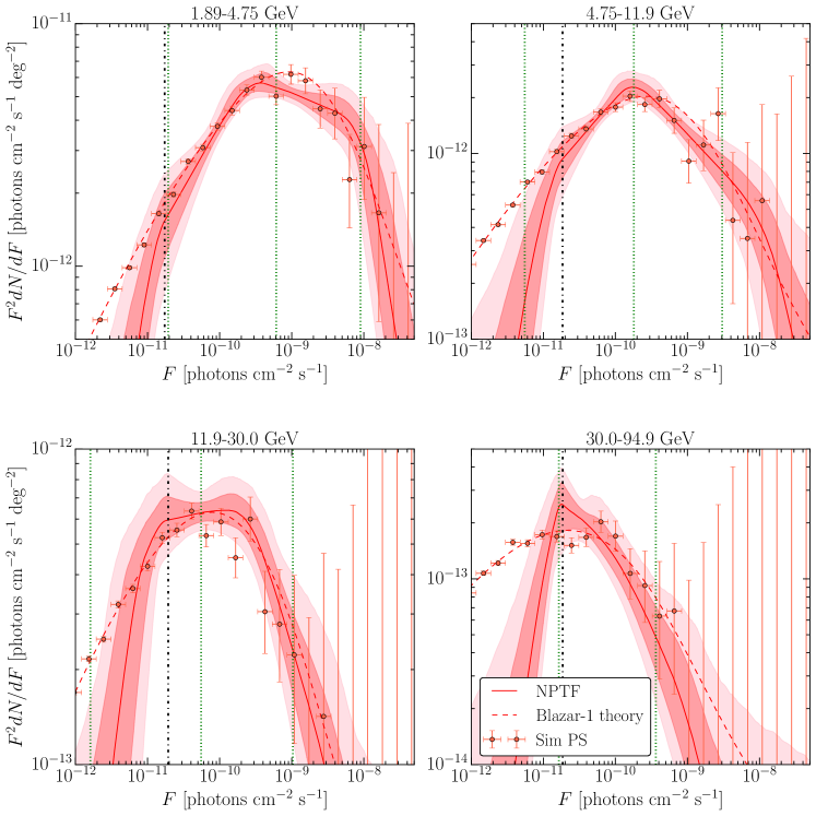
Figure 3.1 shows the best-fit source-count distributions recovered when the NPTF analysis is run on the Blazar–1 simulated data map, assuming the PSF3 instrument response function. In each panel, the dark (light) red band is the 68% (95%) credible interval for the isotropic-PS source-count distribution as recovered from the posterior and constructed pointwise in flux. The red line shows the median source-count distribution, constructed in the same way. The dashed red curve, on the other hand, indicates the source-count distribution of the blazar model used to generate the simulated data. A flux histogram of the simulated PSs for the particular realization shown here is given by the red points, with vertical error bars indicating the 68% credible interval associated with Poisson counting statistics on the number of sources in that bin. Notice that these error bars become large at high fluxes because there are very few sources per flux bin.
In general, the reconstructed source-count distribution is in good agreement with the input source-count distribution at intermediate fluxes, with uncertainties becoming large at low and high fluxes. At high flux, this is due to the fact that it is unlikely to draw a bright source from the underlying source-count distribution. At low fluxes, it is difficult to distinguish PS emission from genuinely isotropic emission. To illustrate this point, we also mark the flux that corresponds to a single photon on average (in the particular energy range, region-of-interest, and event class) with the vertical dot-dashed black line. At fluxes corresponding to counts near or below 1 photon, it is difficult to distinguish PS emission from smooth emission with the NPTF, as evidenced by the growing uncertainties. In this low-flux regime, we do not expect that the NPTF will be able to fully recover the properties of the input source-count distribution.
The vertical dotted green lines in Fig. 3.1 correspond to the fluxes above which 90%, 50%, and 10% (from left to right) of the photon counts are accounted for, on average, by sources with larger flux. Note that in the lowest energy bin, 90% of the flux arises from sources that contribute more than one photon. Moving towards higher energies, a larger fraction of the flux arises from sources that contribute less than one photon. In all energy bins, more than 50% of the flux is accounted for by sources that contribute more than a single photon each.
The corresponding energy spectra for the various templates are shown on the top left panel of Fig. 3.2. As is evident, these blazars show up as PSs under the NPTF; indeed, the smooth isotropic flux (blue) is sub-dominant in each energy bin. Overlaid in dashed red is the spectrum for the simulated Blazar–1 sources. The sum of the smooth and PS isotropic components—which is simply the EGB intensity—is consistent with the simulated spectrum for the blazar model. The green curve shows the median of the posterior for the galactic diffuse model spectrum. The energy spectrum of the diffuse model is softer than that for blazars, so that the diffuse model dominates more at low energies than at high. The sum of the components (yellow band) is consistent with the total flux in the simulated data (black lines) at 68% confidence.
As a contrasting example, we also simulate the Blazar–2 model, which predicts more low-flux sources than the previous example we considered. The best-fit source-count distributions for the Blazar–2 simulated maps are shown in Fig. LABEL:fig:bl2dnds. Once again, we see good agreement between the input data and the recovered source-count distribution above the single-photon sensitivity threshold. In this case, however, the reference model predicts a larger fraction of flux coming from sources below this threshold. For example, about 50% of the flux comes from sub-single photon sources in the second energy bin, and this fraction only increases further at higher energies. The corresponding energy spectrum is shown in the top right panel of Fig. 3.2. As expected, an increasing amount of flux is absorbed by the Poissonian isotropic template. However, the EGB spectrum, shown by the purple band, is still consistent with the input spectrum for the Blazar–2 model.
To further quantify the ability of the NPTF to reconstruct the blazar flux as PS emission, it is convenient to consider the ratios in each energy bin, where is the PS intensity found by the NPTF and is the blazar intensity in the simulation. For the Blazar–1 model, we find‡‡‡‡‡‡Throughout this work, best-fit values indicate the 16, 50, and 84 percentiles of the appropriate posterior probability distributions.
in each of the four respective energy bins, while for the Blazar–2 model, we find
for the particular Monte Carlo realizations shown.******Different Monte Carlo realizations are found to induce variations consistent with the quoted statistical uncertainties, generally on the order of 5%. For the Blazar–2 scenario, more flux goes into smooth isotropic emission, which is why the PS fractions are correspondingly smaller in each energy bin. Note that, in both scenarios, the fraction of the blazar flux absorbed by the PS template decreases at higher energies, where the photon counts become less numerous and a higher fraction of the blazar flux is generated by sub-threshold sources. As a result, the intensities should be interpreted as lower bounds on the blazar flux; this intuition is validated by the fact that the ratios tend to be less than unity.
Next, we explore whether including more quartiles of the ultracleanveto data, as ranked by PSF, increases our ability to reconstruct the blazar flux as PSs under the NPTF. When including more quartiles of data, there are two competing effects that determine our ability to constrain the PS flux: on the one hand, we increase the effective area, but on the other hand, we worsen the angular resolution of the data set. We investigate these effects by repeating the Monte Carlo tests described above using the PSF1–3 instrument response function , and here we simply quote the fractions
for a generic realization of the Monte Carlo simulations for the Blazar–2 model. The PSF1–3 event type increases our ability to distinguish between the blazar emission and smooth emission compared to the PSF3 event type.
3.3.3 Star-Forming Galaxies
Star-forming galaxies (SFGs) like our own Milky Way are individually fainter, though much more numerous, than blazars. The modeling of SFGs in the gamma-ray band is highly uncertain, as Fermi has only detected eight SFGs thus far [269]. However, SFGs could still contribute a sizable fraction of the total flux observed by Fermi. Even though SFGs are PSs, their flux is expected to be dominated by a large population of dim sources degenerate with smooth isotropic emission. Under the NPTF, therefore, we expect that the majority of their emission will be absorbed by the smooth isotropic template. To illustrate this point, we simulate SFGs using the luminosity function and energy spectrum from [224]. In that work, input from infrared wavelengths was used to construct a model for the infrared flux from SFGs. Then, a scaling relation was used to convert from infrared to gamma-ray luminosities. The contributions from quiescent and starburst SFGs were considered separately, along with SFGs that host an AGN. Note, however, that other models predict less emission from SFGs than this particular case—see e.g., [220, 226, 221].
We also performed tests using simulated SFGs. We find that while the NPTF does detect a small PS component in the first few energy bins, as the result of a few SFGs above the sensitivity threshold of the NPTF in those energy bins, by far most of the SFG emission is detected as smooth isotropic emission, with the ratio in all energy bins, where is the intensity of smooth isotropic emission. Moreover, the intensity is consistent with the simulated EGB (SFG flux) in all energy bins, at 68% confidence.
3.3.4 Blazar and SFG combination
A perhaps more realistic scenario for testing the NPTF is to consider a scenario where both SFGs and blazars contribute to the EGB. Therefore, we create simulated maps that include both components and test them on the NPTF. The recovered energy spectra for the SFG + Blazar–1 (Blazar–2) example is shown in the bottom left (right) panel of Fig. 3.2. In both cases, the PS spectrum is consistent with that found in the blazar-only simulations, which are shown in the top panels in that figure. The reconstructed source-count distributions for these examples are not shown, as they are consistent with those found in the blazar-only cases.
In the case of of the Blazar–1 model, the spectra of the smooth isotropic emission and the PS emission trace the spectra of the input SFG population and blazar population, respectively. In the case of the Blazar–2 model, the PS flux is further below the input blazar spectrum, as was found in the blazar-only simulations. However, the smooth isotropic emission is further above the simulated SFG spectrum. In both cases, the sum of the smooth isotropic emission and PS emission (EGB) is consistent with the simulated blazar plus SFG flux.
There is, in fact, a subtle difference between the PS distribution recovered with and without the addition of a SFG population. The difference becomes noticeable when comparing the fractions
for SFG + Blazar–1 and
for SFG + Blazar–2 to the corresponding values for the blazar-only simulations. In the simulations with SFGs, the fractions are generally higher and have larger uncertainties. The reason for this is that the SFG emission is degenerate with an enhanced sub-threshold component to the PS source-count distribution.
Simulating data with the PSF1–3 instrument response function, we find that the ratios are somewhat closer to unity than in the PSF3 case. In particular, for the SFG + Blazar–2 model simulations,
The improved exposure allows the NPTF to probe lower fluxes and to therefore recover a larger fraction of the isotropic-PS emission.
3.4 Low-Energy Analysis: 1.89–94.9 GeV
The findings from the previous section illustrate that the NPTF procedure is able to set strong constraints on the PS (e.g., blazar) and smooth Poissonian (e.g., SFGs, mAGN) contributions to the EGB. In this section, we focus on the energy range from 1.89–94.9 GeV, and begin by presenting the results of our benchmark analysis on the real Fermi data. This is followed by a detailed discussion of potential systematic uncertainties and their effects on the conclusions.
3.4.1 Pass 8 ultracleanveto Data
Top PSF Quartile
We begin by analyzing the ultracleanveto PSF3 data for , using the p8r2 foreground model. This is referred to as the “benchmark analysis” throughout the text. Table 3.2 provides the best-fit intensities for each spectral component, as a function of energy, and the best-fit spectra are plotted in the left panel of Fig. 3.3. The p8r2 diffuse model is shown in green (median only), while the smooth isotropic and isotropic-PS posteriors are shown by the blue and red bands, respectively. The best-fit spectrum for PSs with in the 3FGL catalog [115] is shown by the dashed black line in Fig. 3.3; the spectrum as plotted should be treated with care as systematic uncertainties are not properly accounted for. In particular, the 3FGL catalog includes sources between 0.1–300 GeV. At the high end of this range, the spectrum is driven to a large extent by extrapolations from lower energies, where the statistics are better. The potential errors associated with such extrapolations are difficult to quantify and are not shown in Fig. 3.3. As a result, a direct comparison between the 3FGL spectrum and our results is difficult to make, especially in the highest energy bins. For this reason, we have a dedicated NPTF study for energies greater than 50 GeV in Sec. 3.5. Those results are compared to the Fermi 2FHL catalog [163], which is explicitly constructed at higher energies and is likely a more faithful representation of above-threshold PSs in this regime.
| Energy | |||||
| 1.89–4.75 | |||||
| 4.75–11.9 | |||||
| 11.9–30.0 | |||||
| 30.0-94.9 | |||||
| Energy | |||||||
| 1.89–4.75 | |||||||
| 4.75–11.9 | |||||||
| 11.9–30.0 | |||||||
| 30.0-94.9 | |||||||
The source-count distributions reconstructed from the NPTF are shown in Fig. 3.4, with best-fit parameters provided in Tab. 3.3. For comparison, the binned 3FGL source-count distributions are also plotted; the vertical error bars represent 68% statistical uncertainties and do not account for systematic uncertainties. A few trends are clearly visible. First, each flux break tends to have large uncertainties. This may be a reflection of the fact that the real source-count distribution is not a simple triply-broken power law, but rather a more complicated function, as in the blazar simulations of Sec. 3.3. Therefore, the best-fit values for each of these parameters, when viewed independently, may be somewhat deceptive. As is evident in Fig. 3.4, the posteriors for the breaks and indices are distributed in such a way as to describe a smooth concave function for .
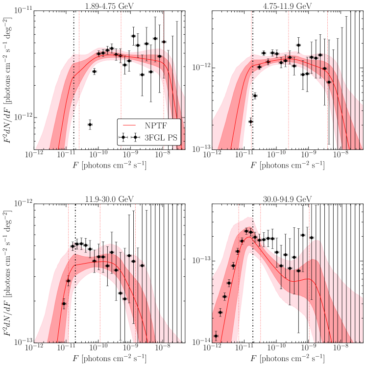
At very high and very low flux, the uncertainties on the indices ( and , respectively) become large. At high flux, this is simply due to the fact that there are very few sources, so the source-count distribution falls off rapidly. At low flux, the large uncertainties on arise from the difficulty in distinguishing the isotropic-PS contribution from its smooth counterpart. Indeed, below the single-photon boundary (dot-dashed black line), the NPTF analysis starts to lose sensitivity. The posterior distributions for the slopes above (below) the highest (lowest) break are highly dependent on the priors and so the quoted values in Tab. 3.3 should be treated with care.
The presence of any distinctive breaks encodes information about the number of source populations as well as their evolutionary properties. In all energy bins, we see that the NPTF places the lowest break, , close to the one-photon sensitivity threshold and the highest break, , in the vicinity of the highest-flux 3FGL source (see Tab. 3.3 for the exact values). The evidence for an additional break, , at intermediate fluxes varies depending on the energy bin. From 1.89–4.75 GeV, there is strong indication for a break at fluxes ph cm-2 s-1, with the index above the break hardening to below the break. In the two subsequent energy bins, up to GeV, we also find evidence that the source-count distribution hardens as we move from high fluxes to below the second break, with the index below the second break 1.9-2.0 in both cases. In the last bin, the uncertainties are too large to determine if the source-count distribution changes slope at any flux above the lowest break .
Top Three PSF Quartiles
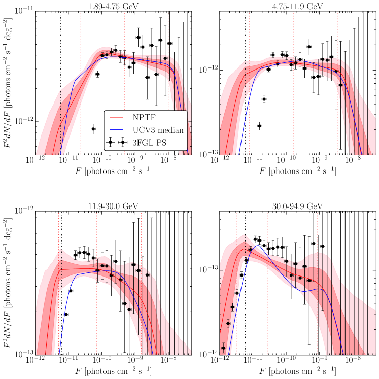
The benchmark analysis described in the previous section used only the top quartile (PSF3) of the Pass 8 ultracleanveto data set. This restriction selects events with the best angular resolution, but at the price of reducing the total photon count. In Sec. 3.3, we showed that including the top three quartiles of the Pass 8 ultracleanveto data may help constrain the source-count distribution at low fluxes. With that in mind, we now investigate how the results of the benchmark analysis change when using the PSF1–3 ultracleanveto data set.
In general, the best-fit intensities for the individual spectral components are consistent within uncertainties with those obtained using only the top quartile of data. The PS flux does increase slightly in going from PSF3 to PSF1–3 in the upper energy bins due to the increased exposure. More specifically, the ratios of the median PS intensities measured with ultracleanveto PSF1–3 data to those measured with PSF3 data are in the four increasing energy bins. This can also be seen in the associated spectral intensity plot (right panel of Fig. 3.3), where the red bands are further above the 3FGL line in the last energy bins than in the corresponding plot for the PSF3 analysis (left panel). The intensity of the EGB is seen to increase slightly, in all energy bins, when going from PSF3 to PSF1–3 data, potentially suggesting additional cosmic-ray contamination with the looser photon-quality cuts, though the increases in EGB intensities are within statistical uncertainties.
The best-fit source-count distributions recovered by the NPTF with PSF1–3 data are shown in Fig. 3.5. For reference, the blue curve shows the best-fit for the PSF3–only analysis. The most important difference between the PSF3 and PSF1–3 results is that the source-count distributions extend to lower flux with PSF1–3 data. This is due to the fact that the exposure in each energy bin, averaged over the region of interest, is larger for the top three quartiles compared to the top quartile alone. As a result, the flux corresponding to single-photon detection is lower (compare the vertical dot-dashed line in Fig. 3.5 with that in Fig. 3.4), which improves the NPTF reach. Thus, the PSF1–3 analysis is sensitive to more sub-threshold sources. Note that the same trend was observed in the simulation tests in Sec. 3.3 in going from PSF3 to PSF1–3 data sets.
Other than the location of the lowest break, which is lower due to the increased exposure, all other source-count distribution parameters are consistent, within uncertainties, between analyses. At the lowest energy, the break at photons cm-2 s-1 is even more pronounced, with an index above the break and below the break. In the highest energy bin, the structure observed in the source-count distribution for the benchmark analysis has smoothed out.
3.4.2 Systematic Tests
The previous subsection illustrated how the results of the NPTF change when additional ultracleanveto PSF quartiles are included in the analysis. We also tested the stability of our analysis to variations in the region of interest, Fermi event class, foreground modeling, Fermi bubbles, PSF modeling, and choice of priors.
Figure 3.6 briefly summarizes the results. The EGB intensity as measured by Fermi is shown by the gray band. To obtain this band, we use the best-fit power-law spectrum with exponential cut-off provided in [199]; the width of the gray band is found by varying between best-fit values for the three foreground models considered in that paper (Models A/B/C) and does not include statistical uncertainties, which become increasingly important at high energies. The smooth isotropic intensity, and thus the intensity of the EGB, is subject to large systematic uncertainties. As expected, the variation in smooth isotropic intensity is most pronounced when using the source event class, which contains more cosmic-ray contamination. However, the spectrum of emission from PSs as captured by the NPTF appears robust to all the systematic effects considered here. This is the primary conclusion of this subsection. We now describe in detail the systematic tests that were conducted for the low-energy analysis.
Region of Interest
As a first cross-check on the stability of the results presented in Sec. 3.4.1, we explore the effects of altering the region of interest. While we previously defined the region of interest with , we now loosen this constraint and consider the case . Extending the region of interest closer to the Galactic disk increases the amount of data being analyzed, but at the cost of potentially more contamination from diffuse foreground emission and local PSs. As shown in Fig. 3.6, the best-fit intensities for the isotropic and isotropic-PS components are equivalent, within errors, to their counterparts in the benchmark analysis.
We also ran the NPTF on the Northern () and Southern () hemispheres separately. The intensities for the EGB, IGRB, and PS components are systematically lower (higher) for the Northern (Southern) analysis than for the benchmark case.
Event class
We explored the implications of broadening the ultracleanveto data set to include the top three quartiles in Sec. 3.4.1. Now, we consider the implications of repeating the NPTF analysis on the source data with PSF1–3. This event class has looser photon-quality cuts, which leads to larger overall exposure, but significantly more cosmic-ray contamination. In general, it is not recommended to use source data for IGRB studies; for our purposes, however, it will be intriguing to see how the increased photon statistics affect the recovered source-count distribution for the PS component. As shown in Fig. 3.6, the EGB intensity is far larger than that recovered by the benchmark analysis and overpredicts Fermi’s EGB result in most energy bins. The sharp rise in the EGB intensity can be traced to a substantial fraction of smooth isotropic emission, which is expected for this event class at most energies. Most importantly, the intensity of the isotropic-PS component is consistent, within uncertainties, with that found in the benchmark analysis.*†*†*†The recovered PS intensity is slightly larger with source PSF1–3 data as compared to ultracleanveto PSF3 data, which is likely due to the increased exposure in the source PSF1–3 data set. This is a confirmation that the NPTF is able to successfully constrain the source-count distribution even in a data set with significantly more smooth isotropic flux.
Foreground Model
A potentially significant source of systematic uncertainty in the NPTF analysis is due to mis-modeling of high-energy gamma-rays produced in cosmic-ray propagation in the Milky Way [270]. These high-energy photons arise from bremsstrahlung of electrons off the interstellar medium, boosted pion decay, and inverse Compton (IC) emission off the interstellar radiation field. Our benchmark analysis uses the associated foreground model for the Pass 8 data set (gll_iem_v06.fits), denoted here as p8r2. The total diffuse emission in p8r2 is modeled as a linear combination of several sources, some of which are traced by maps of gas column densities, which serve as templates for the pion and bremsstrahlung emission. The IC component is modeled using the GALPROP package [271].*‡*‡*‡http://galprop.stanford.edu/ These individual templates are fit to the data, and used to identify ‘extended emission excesses’ that are identified directly and then added back into the model [272].
To better assess the uncertainties due to the foreground modeling, we repeat the NPTF analysis using several other foreground models made available by Fermi. In particular, we use the gll_iem_v02_P6_V11_DIFFUSE.fits diffuse emission model, denoted as p6v11, which was initially developed for the Pass 6 data set.*§*§*§http://fermi.gsfc.nasa.gov/ssc/data/access/lat/ring_for_FSSC_final4.pdf p6v11 is distinct from p8r2 in that it uses older gas and IC maps and does not include templates for large-scale structure or extended emission excesses. The Pass 7 model gal_2yearp7v6_v0.fits, denoted as p7v6,*¶*¶*¶http://fermi.gsfc.nasa.gov/ssc/data/access/lat/Model_details/Pass7_galactic.html is a compromise as it uses updated gas and IC maps and includes some large-scale extended structures, such as Loop 1 and the Fermi bubbles.
The NPTF results using the p6v11 and p7v6 foreground models are summarized in Fig. 3.6.In general, we observe that the intensity of the PS components is consistent with that for the benchmark analysis in all energy bins. However, variations occur in the smooth isotropic intensity. Typically, more IGRB intensity is recovered with p6v11 and p7v6, versus p8r2. The differences are particularly dramatic in the first two energy bins and are more severe for p6v11. The net consequence is that the EGB intensity is higher than the expected range from Fermi. The enhancement in the isotropic component may arise from the fact that each foreground model incorporates large-scale diffuse structures differently—with p6v11 being the least inclusive and p8r2 being the most inclusive. We note, however, that the fit to data with the p8r2 foreground model, from the point of view of the Bayesian evidence, is much better than the analogous fit with the p6v11 model; the fit with the p7v6 model is intermediate.
The Bubbles Template
To better understand how dependent the analysis is on the details of the Fermi bubbles template, we simply removed the template from the analysis. This has indiscernible effects on the final results. We see in Fig. 3.6 that the EGB, IGRB, and PS intensities are consistent, within uncertainties, to the corresponding values in the benchmark study.
Point Spread Function
The PSF can affect the photon-count distribution because it can redistribute photons between pixels, and must therefore be properly accounted for in the calculation of the photon-count probability distributions. For the primary analyses presented in this work, the PSF is modeled using a King function. However, to test the sensitivity of the results to mis-modeling of the PSF, we have also repeated the NPTF analysis using a two-dimensional Gaussian in the calculation of the photon-count probability distributions, with a width set to give the correct 68% containment radius. As shown in Fig. 3.6, the NPTF results remain unchanged with this substitution.
Priors
Our choice of priors, given in Tab. 3.1, is carefully chosen to both avoid biasing the posterior for the source-count distribution while at the same time allowing breaks at both high and low flux. This is meant to properly account for the fact that the source-count distribution is not well constrained by the data at very high fluxes, where the mean expected number of sources over the full region is much less than unity, and at very low fluxes, where the mean photon-count per source is much less than unity. Our choice of priors is further justified by the simulated data studies, presented in Sec. 3.3, which show that the NPTF can successfully constrain the emission from blazar models. However, one may still be concerned that these particular choice of priors might bias the recovered source-count distribution in a particular way. For that reason, we have tried many variations to the priors shown in Tab. 3.1, three of which (labeled ‘Alt. priors 1–3’) are described below and shown in Fig. 3.6:
-
•
Alternate prior 1: All priors are the same as in Tab. 3.1, except for those on the breaks, which are changed to , , and ph for , , and , respectively.
-
•
Alternate prior 2: As above, except changing the priors for the breaks to , , and ph, respectively.
-
•
Alternate prior 3: All priors are the same as in Tab. 3.1, except for that of , which is changed to .
The first two examples address the possibility that the break priors might artificially sculpt the source-count distribution and the recovered PS intensity, while the third example addresses how the source-count distribution is dealt with at fluxes below the lowest break, where the distribution is not well constrained by the data. In many classes of blazar models, such as those considered in Sec. 3.3, the index below the lowest break () is greater than unity, so that the total number of PSs diverges as the minimum flux cut-off is taken to zero.
It is useful to know if the recovered PS intensity, , tends to under or overshoot the simulated blazar intensity, , when using the alternate priors. With that in mind, we run the NPTF on simulated maps, as in Sec. 3.3, constructed from both the SFG + Blazar–1 model as well as the SFG + Blazar–2 model. For Alternate prior 1, we find that
and
for the SFG + Blazar–1 and SFG + Blazar–2 models, respectively, with ultracleanveto PSF3 instrument response function. With Alternate prior 1, we see larger uncertainties, with the PS template capable of absorbing more flux in particular. With Alternate prior 2, on the other hand, we find more noticeable differences in the medians as well as in the uncertainties. In particular, for the SFG + Blazar–1 and SFG + Blazar–2 models, we find
and
respectively. In the Blazar–1 model case, it is important to notice that at intermediate energies the NPTF tends to over-predict at the 20% level. With Alternate prior 3, the results are
and
for the Blazar–1 and Blazar–2 models. The Alternate prior 3 results are consistently closer to unity than the first two alternate prior results.
As may be seen in Fig. 3.6, the median values for the PS intensities recovered from the NPTF analyses with alternate priors are generally consistent with those found in the baseline study. The Alternate prior 3 PS intensities are slightly enhanced in all energy bins compared to the baseline results—following our expectations from the simulation results presented above—though the two results are consistent within statistical uncertainties.
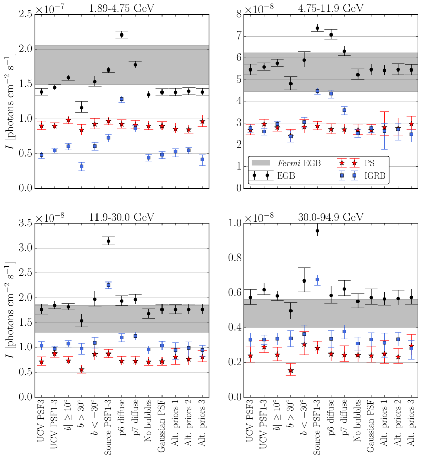
3.5 High-Energy Analysis: 50–2000 GeV
We now consider the NPTF results at high energies from 50–2000 GeV. The number of photons available decreases when moving to higher energies, so we loosen the restrictions on the PSF quartiles to maximize the sensitivity potential of the NPTF. In this section, the majority of the analyses are done using all quartiles of the ultracleanveto data, though we also show results using all quartiles of source data. For the same reason, we widen the ROI to rather than , although the results are not sensitive to this cut, as we will show.
The best-fit energy spectra recovered by the NPTF analysis for the high-energy study of ultracleanveto data is shown in the bottom right panel of Fig. 3.7. The fit results are compared with the best-fit energy spectrum for sources in Fermi’s 2FHL catalog [214] (dashed black line). This recently-published catalog is based on 80 months of data and focuses on hard sources in the range from 50–2000 GeV. Statistical and systematic uncertainties are not accounted for in the determination of the 2FHL spectrum in Fig. 3.7; these are likely non-negligible, especially at the highest energies.
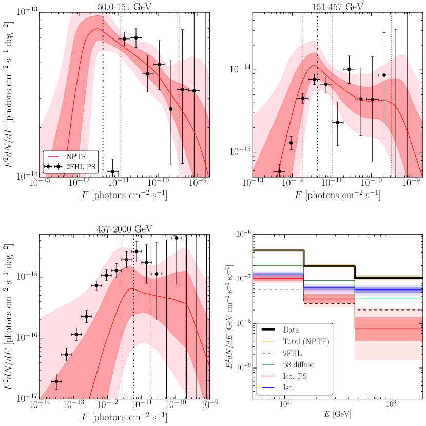
The best-fit source-count distributions for the three energy bins are also shown in Fig. 3.7, in the top row and bottom left panel. The black points in those panels denote the 2FHL source-count distributions, with vertical error bars indicating 68% Poisson errors. The statistical errors on the 2FHL sources are large due to the fact that there are not many sources. In all energy bins, the NPTF places the lowest break close to the single-photon sensitivity threshold (vertical dot-dashed line) and the highest break in the vicinity of the brightest 2FHL source, just as in the low-energy analysis. Most notably in the 50–151 GeV bin, the NPTF probes unresolved sources with fluxes nearly an order-of-magnitude below the apparent 2FHL threshold. We find no evidence for an additional intermediate-flux break in any of the energy bins, although it is difficult to make conclusive statements due to the large uncertainties in the individual source-count distributions.
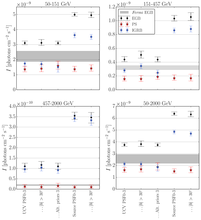
We have completed a number of systematic tests of the high-energy analyses that include looking at all quartiles of the source data, requiring for both event classes, and using the third alternate prior choice, with . The results are summarized in Fig. 3.8. Importantly, the isotropic-PS intensity is consistent across all the tests. However, the EGB intensities recovered by the NPTF are, in general, higher than those measured by Fermi. This discrepancy is likely due to increased cosmic-ray contamination above 100 GeV, as suggested by the high IGRB intensities recovered by the NPTF at these energies. Indeed, the Fermi EGB study on Pass 7 data [199] used dedicated event classes with specific data cuts to minimize such contributions. Such an analysis is beyond the scope of this study, as our primary focus is on the PS populations. We simply caution the reader that the derived intensity for the smooth isotropic component in the high-energy analyses is subject to potentially large contamination.
It is possible to make stronger statements about the best-fit source-count distribution at high energies if we consider the wide-energy bin from 50–2000 GeV. The results are shown in the left panel of Fig. 3.9. Due to the improved statistics, the uncertainties on the source-count distribution are smaller than those for the three sub-bins. Other than the low-flux sensitivity break, the NPTF finds no preference for an additional break. The intermediate-flux break, , is essentially unconstrained as a result, and the power-law slope above (below) it are consistent within uncertainties: and , respectively. We compare this result to the best-fit source-count distribution (blue line) published by Fermi for sources in this same energy range [163]. There are important differences between the two analyses. In the Fermi study, simulated maps were created using several different source-count distributions, parametrized as singly broken power laws. The histogram of the photon-count distribution for each of these maps, averaged over the full region of interest, was compared to the actual data, and a fit was done to select the simulated maps that most closely resembled the data. This method is related to but in many ways distinct from the NPTF. The NPTF considers the difference between Poissonian and non-Poissonian photon probability distributions at the pixel-by-pixel level, instead of averaging the distributions over the full region. Moreover, in our analysis we rely on semi-analytic techniques to calculate the photon-count probability distributions as we scan over the space of model parameters, instead of relying on Monte Carlo samples to numerically construct these distributions. As a result, we are able to consider source-count distributions with additional degrees of freedom and also scan over the normalizations of all of the background templates, which tend to be well determined given the pixel-by-pixel nature of the fit. In contrast, the intensity of all Poissonian models in [163], including the smooth isotropic emission, was kept fixed while scanning over the source-count distribution degrees of freedom.
The cumulative source-count plot is provided in the right panel of Fig. 3.9. Our result is in good agreement with the 2FHL sources above the catalog sensitivity threshold ph cm-2 s-1. In the first few flux bins above this threshold, there appear to be more 2FHL sources than what is predicted by the NPTF, although the results are still consistent within uncertainties. This may be due to the Eddington bias [273] where extra sources are observed above threshold due to upward statistical fluctuations from sources immediately below.
Based on the results in Fig. 3.9, we can project the expected number of these sources that may be observed by the Cherenkov Telescope Array (CTA) [246, 247]. For energies above 50 GeV, the CTA flux sensitivity is cm-2 s-1 for 50 hours of observation per field-of-view (5 detection).*∥*∥*∥https://portal.cta-observatory.org/Pages/CTA-Performance.aspx For 250 hours total of observation time, this covers 190 deg2 of sky, assuming a field-of-view. As shown in Fig. 3.9, the NPTF predicts a density of deg-2 for sources above this threshold. This translates to detected sources, more than double what had previously been estimated for similar observing parameters [247]. Relaxing the observing time per source and assuming, as in [163], that a quarter of the sky is surveyed in 240 hours at 5mCrab sensitivity, then the NPTF predicts sources. This is lower, and in slight tension, with the sources predicted by the Fermi study using the blue source-count distribution illustrated in Fig. 3.9.
3.6 Discussion and Conclusions
The primary focus of this chapter is to characterize the properties of the PSs contributing to the EGB in a data-driven manner. To achieve this, we use a novel analysis method, referred to as Non-Poissonian Template Fitting (NPTF), which takes advantage of photon-count statistics to distinguish diffuse and PS contributions to gamma-ray maps with non-trivial spatial variations. We presented the NPTF results on Fermi Pass 8 data at low (1.89–94.9 GeV, ) and high (50–2000 GeV, ) energies. For the first time, the intensity and source-count distributions for the isotropic PSs have been obtained as a function of energy, up to 2 TeV. The best-fit source-count distributions probe fluxes below the current detection threshold for the Fermi 3FGL and 2FHL catalogs, providing information on the unresolved populations.
Through extensive studies of how the NPTF responds to simulated populations, we have shown that the analysis procedure reproduces the properties of input source classes. Therefore, the features of the best-fit source-count distributions obtained from the data provide a potential wealth of information about the source populations of the EGB. While a detailed interpretation of the source-count distributions in terms of particular theoretical models is beyond the scope of this study, several important trends were observed.
In this chapter, the source-count distributions are parametrized as triply-broken power laws in the NPTF. At all energies, a break is fit at low (high) fluxes, below (above) which the analysis method loses sensitivity. Of particular interest is whether an additional break, , is preferred at intermediate flux. We find a break in the lowest energy bin (1.89–4.75 GeV) at cm-2 s-1 with slope above and below. In the subsequent two energy bins, 4.75–11.9 GeV and 11.9–30.0 GeV, there is a mild indication that the source-count distribution hardens below the intermediate flux break, though the change in slope is not as robust and significant as in the lowest energy bin. At higher energies, above 30 GeV, there is no indication that the source-count distribution changes slope at the intermediate break. This trend is in line with the expectations from the blazar simulations in Sec. 3.3. For example, in both Figs. 3.1 and LABEL:fig:bl2dnds, which show the results of the NPTF run on simulated data with the Blazar–1 and Blazar–2 models, we find evidence for curvature in the source-count distribution at intermediate fluxes in the lowest energy bins, while at higher energies the recovered source-count distribution appears as a single power law at fluxes above the sensitivity threshold of the NPTF. In the energy bin from 50–2000 GeV the best-fit value for is essentially unconstrained and the slopes above and below it are consistent within uncertainties: and .
The NPTF also provides the best-fit intensities for the isotropic-PS populations as a function of energy. Figure 3.10 illustrates this spectrum for analyses done using the ultracleanveto event class. The filled red circles (open red boxes) show the results for the dedicated low (high)-energy analysis, with PSF1–3 data used at low energies and PSF0–3 data at high energies. For comparison, the Fermi EGB spectrum is shown by the black line [199]. This corresponds to the best-fit intensity using the Model A diffuse background from that study. To illustrate the systematic uncertainty on this curve, we also plot the spectra for diffuse models B and C (dashed and dotted, respectively).
| Low-Energy Analysis | High-Energy Analysis | |||||||
| 1.89–4.75 | 4.75–11.9 | 11.9–30 | 30–94.9 | 50–151 | 151–457 | 457–2000 | 50–2000 | |
| Scenario A | ||||||||
| Scenario B | ||||||||
The PS fraction, defined as , is provided in Tab. 3.4 for each energy bin. While using the EGB intensity derived in this study (‘Scenario A’) is the most self-consistent comparison, this may underestimate the PS contribution above 100 GeV, where the NPTF appears to recover too much smooth isotropic emission due to increased cosmic-ray contamination in the data sets used, as already discussed. Therefore, we also show the PS fractions calculated relative to the Fermi EGB intensity from [199] for diffuse model A (‘Scenario B’). The comparison to the EGB as measured in [199] is not fully self consistent, since, for example, the foreground modeling and data sets in [199] differ from those used in this study to measure . However, the advantage of this comparison is that the Fermi analysis uses special event-quality cuts to mitigate contamination, and thus their measure of is likely more faithful than that presented in this study. These results are shown in the second row of Tab. 3.4. For the low-energy analysis, the PS fractions are consistent, within uncertainties, when is taken from our study or Fermi’s.*********For ‘Scenario B’, the quoted uncertainties only include those measured in this work for . For , we use the best-fit value given in [199]. The substantial differences occur at high-energies, where our result is systematically lower than the fractions based on Fermi’s EGB intensity.
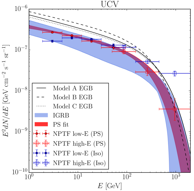
In general, we find that approximately 50–70% of the EGB consists of PSs in the energy ranges considered. To interpret these results, we use the ratios obtained in the simulation studies of Sec. 3.3. In that section, we showed that the efficiency for the NPTF to recover the flux for the Blazar–2 model (with PSF1–3) is 100% in the first energy bin and drops to 60% in the fourth energy bin. For the Blazar–1 model, the efficiencies are consistently higher than the Blazar–2 scenario. These two blazar models are meant to illustrate extreme scenarios, with the Blazar–1 model having a significant fraction of the total flux arising from high-flux sources, while low-flux sources dominate instead in the Blazar–2 case. The high efficiency of the NPTF to recover the blazar component at low energies, combined with the PS fractions observed in the data (Tab. 3.4), clearly suggests that there is a substantial non-blazar component of the EGB up to energies 30 GeV. The interpretation of the results in the energy bin from 30.0–94.9 GeV is less clear. A proper interpretation of the results at higher energies in terms of evidence for or against a non-blazar component of the EGB requires dedicated blazar simulations, which we leave to future work.
Our results tend to predict fewer PSs (and photons from PSs) where we do overlap with previous studies. For example, a similar photon-count analysis was used by [162] to study 1–10 GeV energies in the Pass 7 Reprocessed data. They found an 80% PS fraction at these energies. At the lowest energies that we probe—which admittedly do not extend down as low as 1 GeV—we only find a 54% PS fraction (relative to Model A). Systematic uncertainties, as shown in Fig. 3.6, can affect the recovered PS intensities at the level, which can partially alleviate the tension between our results.
Above 50 GeV, the NPTF procedure predicts that of the EGB consists of PSs, with systematic uncertainties estimated at approximately . This fraction is smaller, and in slight tension, with the predicted value obtained in previous work [163]. The fact that our results suggest that there is more diffuse isotropic emission at high energies may help alleviate the tension between [163] and the hadronuclear () interpretation of IceCube’s PeV neutrinos [230]. Some models suggest, for example, that these very-high-energy neutrinos are produced in hadronuclear interactions, along with high-energy gamma-rays that would contribute to the IGRB [230, 224, 244, 229]. If the smooth isotropic gamma-ray spectrum (i.e., the non-blazar spectrum) is suppressed above 50 GeV in the Fermi data, it could put such scenarios in tension with the data [171, 274]; however, that does not necessarily appear to be the case given the results of our analysis [172]. With that said, and as already mentioned, dedicated blazar simulations at high energies are needed to properly interpret our results at these energies.
The PS spectrum in Fig. 3.10 is well-modeled (reduced ) as a power law with an exponential cut-off:
| (3.13) |
where GeV-1cm-2s-1sr-1, , and GeV are the best-fit parameters.*††*††*††Repeating the fit using the results from the NPTF analyses with source data returns similar results, though the PS spectrum is slightly enhanced relative to the ultracleanveto result. In particular, with source data, we find GeV-1cm-2s-1sr-1, , and GeV, with reduced . Note that the fit is done taking into account the uncertainties on the PS intensities in the energy sub-bins. The global fit for the PS spectrum is shown in Fig. 3.10 by the red band, which denotes the 68% credible interval. Interestingly, the index and cut-off that we extract from the fit are very similar to the values found in [199], which used the same functional form to fit the EGB spectrum. Subtracting our PS spectrum from the EGB spectral fits gives the blue band in Fig. 3.10. The band includes statistical uncertainties from our global fit as well as systematic uncertainties associated with varying between Models A-C. The blue band is an estimate of the IGRB spectrum and we compare it to the smooth isotropic spectrum recovered by the NPTF (blue points). Note that the two are consistent, within the large uncertainties, below 100 GeV; above this energy, our IGRB value is expectedly high.
The NPTF allows us to make statistical statements about the properties of source populations contributing to the EGB, but at the expense of identifying the precise locations of these sources. However, it is still possible to make probabilistic statements about these locations. To do so, we compare the observed photon count in a given pixel, , to the mean expected value, , without accounting for PSs. To determine we include the diffuse background, smooth isotropic emission, and the Fermi bubbles templates, with normalizations as determined from the NPTF. The pixel-dependent survival function is defined as
| (3.14) |
where CDF is the Poisson cumulative distribution function. The smaller the value of (or, conversely, the larger the value of ), the more probable it is that the pixel contains a PS. Figure 3.11 shows full-sky maps of for both low (1.89–94.9 GeV) and high (50–2000 GeV) energies.*‡‡*‡‡*‡‡ Digital versions of these maps are available upon request. The white circles indicate the presence of a 3FGL (2FHL) source for the low- (high-)energy map, with the radii proportional to the predicted photon counts for the sources. There is good correspondence between the hottest pixels, as determined by , and the brightest resolved sources. Pixels that are correspondingly less “hot” tend to be associated with less-bright 3FGL (or 2FHL) sources. Of particular interest are the hot pixels not already identified by the published catalogs. In the region () in the low- (high-)energy analysis, these are likely the sources lending the most weight to the NPTF below the catalog sensitivity thresholds. While more sophisticated algorithms are needed to further refine the candidate source locations, Fig. 3.11 provides a starting point for identifying the spatial locations of potential new sources to help guide, for example, future TeV gamma-ray observations and cross-correlations with other data sets, such as the IceCube ultra-high-energy neutrinos.
Deciphering the constituents of the EGB remains an important goal in the study of high-energy gamma-ray astrophysics, with broad implications extending from the production of PeV neutrinos to signals of dark matter annihilation or decay. The Fermi LAT has already played an important role in the discovery of many new sources in the GeV sky. By taking advantage of the statistical properties of unresolved populations, our results provide a glimpse at the aggregate properties of the sources that lie below the detection threshold of these published catalogs and suggest a wealth of detections for future observatories.
3.6.1 Implication for Dark Matter Annihilation Searches
Pinning down the origin of 50-70% of the extragalactic gamma-ray sky as being of point source origin narrows down the potential contribution of more exotic sources such as the integrated emission of annihilating dark matter in halos around far-away galaxies and clusters. This would lead to an improvement in constraints on annihilating DM obtained by studying their contribution to the isotropic gamma-ray background (IGRB), such as those presented in [117, 118], potentially by a factor of a few.
There are a few drawbacks to this approach, however. The contribution of relatively nearby halos to an annihilation signal is expected to dominate due to the late-time clustering of matter (which boosts the annihilation signal) as well as our favored location in the Local Group where we are surrounded by halos and clusters of a larger size than those around a randomly chosen place in the Universe. This fact is not optimally taken into account in IGRB analyses. Secondly, IGRB analyses for dark matter annihilation cannot conclusively discover a DM signal due to the irreducible isotropic background of astrophysical origin – only constraints on its properties are possible.
In the next part of this thesis, we will systematically build up the best way to search for extragalactic dark matter annihilation, focusing on emission from nearby galaxies and clusters. We will develop a framework to characterize the distribution of nearby extragalactic dark matter halos (Ch. 4) and look for this structure in Fermi data (Ch. 5).
Chapter 4 Mapping Extragalactic Dark Matter Annihilation with Galaxy Surveys
This chapter is based on an edited version of Mapping Extragalactic Dark Matter Annihilation with Galaxy Surveys: A Systematic Study of Stacked Group Searches, Phys.Rev. D97 (2018) 063005 [arXiv:1709.00416] with Mariangela Lisanti, Nicholas Rodd, Benjamin Safdi and Risa Wechsler [131]. The results of this chapter have been presented at the following conferences and workshops: TeV Particle Astrophysics (TeVPA) 2017 in Columbus, OH (August 2017), Dark Matter, Neutrinos and their Connection (DACO) in Odense, Denmark (August 2017), Workshop on Statistical Challenges in the Search for Dark Matter in Banff, Canada (February 2018) and Recontres de Blois 2018 in Blois, France (June 2018).
4.1 Introduction
Dark matter (DM) annihilation into visible final states remains one of the most promising avenues for discovering non-gravitational interactions in the dark sector. While an individual annihilation event is rare, the probability of observing it can be maximized by searching for excess photons in regions of high dark matter density. The center of the Milky Way is potentially one of the brightest regions of DM annihilation as seen from Earth, but the astrophysical uncertainties associated with the baryonic physics at the heart of our Galaxy motivate exploring other targets. Gamma-ray studies of DM-dominated dwarf galaxies in the Local Group currently provide some of the most robust constraints on the annihilation cross section [89, 90]. However, many more potential targets are available beyond the Local Group. This chapter proposes a new analysis strategy to search for DM emission from hundreds more DM halos identified in galaxy group catalogs.
A variety of methods have been used to study gamma-ray signatures of extragalactic DM annihilation, including modeling potential contributions to the Isotropic Gamma-Ray Background [231, 232, 233, 234, 43, 235, 118, 120, 117, 275], measuring the Fermi auto-correlation power spectrum [276, 277, 278, 279], and cross-correlating the Fermi data with galaxy counts [280, 281, 122, 121, 126, 125, 124, 123], cosmic shear [282, 130, 283, 284, 128, 127, 129] and lensing of the Cosmic Microwave Background [285, 275]. These methods typically rely on using a probabilistic distribution of the DM annihilation signal on the sky. Our approach is more deterministic in nature. In particular, we treat a collection of known galaxies as seeds for DM halos. The properties of each galaxy—such as its luminosity and redshift—enable one to deduce the characteristics of its associated halo and the expected DM-induced gamma-ray flux from that particular direction in the sky. In this way, we can build a map of the expected DM annihilation flux that traces the observed distribution of galaxy groups.
In certain ways, our approach resembles that used in previous studies of DM annihilation from individual galaxy clusters. For example, most recently the Andromeda galaxy [286] and Virgo cluster [116] have been the subject of dedicated study by the Fermi Collaboration. Other work has inferred the properties of the DM halos associated with galaxy clusters detected in X-rays [287, 288, 289, 290, 291, 292, 293]. Most of these studies focused on a small number of galaxy clusters and obtained DM sensitivities weaker than those from dwarf galaxies.
Recent advancements in the development of galaxy group catalogs allow us to now build a full-sky map of the nearby galaxies that should be the brightest DM gamma-ray emitters. Catalogs based primarily on the 2MASS Redshift Survey (2MRS) [294] provide an unprecedented amount of information regarding a group’s constituents and halo properties [132, 133, 295]. This information allows us to build a list of the brightest extragalactic DM targets on the sky and to perform a stacked analysis for gamma-ray emission from them. A gamma-ray line search using this methodology was recently performed by Ref. [296]. Our focus is on continuum DM signatures, which carry considerably more complications in terms of the treatment of astrophysical backgrounds.
In the upcoming Chapter 5, we present results implementing a stacked analysis of the group catalogs from Ref. [132, 133] on Fermi data and show explicitly that this method yields competitive sensitivity to the dwarf searches. Here, we present the full details of the analysis method and a thorough discussion of the systematic uncertainties involved in deducing the DM-induced flux associated with a given galaxy group. To fully understand these uncertainties, we apply these methods on mock data where it is possible to compare the inferred DM properties to their true values. For this purpose, we use the DarkSky cosmological -body simulation [297, 298] and an associated galaxy catalog from Ref. [298]. We emphasize that, while we illustrate the analysis method on gamma-ray data, it can also be applied to other wavelengths and even other messengers, such as neutrinos.
This chapter is organized as follows. In Sec. 4.2, we describe how to build DM annihilation flux maps starting from a galaxy group catalog and discuss the associated systematic uncertainties. Sec. 4.3 presents a detailed description of the statistical methods that we follow to implement the stacking. We show the results of applying the limit-setting and signal recovery procedures on mock data in Sec. 4.4 and conclude in Sec. 4.5. Appendix A provides a detailed discussion of the -factor expressions used in the main text.
4.2 Tracing Dark Matter Flux with Galaxy Surveys
In this Section, we describe how to construct catalogs of extragalactic DM targets starting from a list of galaxy groups. We begin by reviewing the properties of the galaxy group catalogs and then describe how to predict the DM signal from a given galaxy group and quantify the systematic uncertainties of this extrapolation.
4.2.1 Galaxy and Halo Catalogs
The approach that we use throughout this work relies on galaxy surveys as an input. Different galaxy catalogs span a range of redshifts and luminosities. Optimal catalogs for DM searches should cover as much of the sky as possible (to increase statistics) and sample low redshifts (). The strength of the DM signal increases at lower redshifts due to accretion of mass at late times, affecting both the halo mass distribution and substructure [122]. In contrast, the integrated gamma-ray flux of standard astrophysical sources, such as Active Galactic Nuclei and star-forming galaxies, is expected to peak at higher redshifts between 0.1 and 2 depending on the specific source class and model for its unresolved contribution [122, 126].
The Two Micron All-Sky Survey Extended Sources Catalog (2MASS XSC) [299, 294] satisfies the criteria listed above and has been used extensively in past cross-correlation studies [121, 122, 123, 124, 125, 281, 126]. The XSC is an all-sky infrared survey that consists of approximately one million galaxies up to a limiting magnitude of mag. Several redshift surveys based on the 2MASS XSC map the redshifts associated with these galaxies. The 2MRS [294], for example, samples about 45,000 galaxies in the 2MASS XSC with redshifts to a limiting magnitude of mag. This corresponds to a nearly complete galaxy sample up to redshifts of , which is ideal for DM studies.
Galaxies from large surveys such as 2MASS can be organized into group catalogs. A group of gravitationally-bound galaxies shares a DM host halo. The brightest galaxy in the group is referred to as the central galaxy; the additional galaxies are bound satellites surrounded by their own subhalos. As we will see, the total luminosity of the galaxies in the group is a good predictor of the mass of the DM host halo. A variety of group finders have been developed and applied to the 2MASS data set [132, 295, 133], using the 2MRS which adds information in the redshift dimension. The groups in these catalogs range from cluster scales with 190 members and associated halo masses of 1015 M⊙, down to much smaller systems with only a single member. Galaxy group catalogs are especially relevant for the present study, since (as will be shown) halo properties tend to be correlated with properties of galaxy groups rather than those of individual galaxies.
While in the upcoming Chapter 5 we use information from the 2MASS group catalogs in the analysis of Fermi data, we focus on a catalog of simulated galaxies and halos here. We use the DarkSky-400 cosmological -body simulation (version ds14_i) [297, 298] and an associated -band galaxy catalog. Using the code 2hot [300], DarkSky-400 follows the evolution of particles (DM-only) of mass M⊙ in a box 400 Mpc per side. Initial perturbations are tracked from to today, assuming . The halo catalog was generated using the Rockstar halo finder [301, 298]. Crucially, the simulation covers the relevant redshift space for DM studies.***The snapshot of the simulation analyzed in this work is taken at , but we will refer to distance using redshift because that is the more appropriate language when applied to real data. In particular, an observer at the center of the simulation box has a complete sample of galaxies out to , with the furthest galaxies extending out to . In our work, we only consider groups located within , which is the approximate redshift cutoff of the catalogs in Ref. [132, 133, 295]. We include only well-resolved halos in our analysis by imposing a lower cut-off of M⊙ on the mass of included host halos. The associated galaxy catalog is generated using the abundance matching technique following Ref. [302, 303] with luminosity function and two-point correlation measurements from the Sloan Digital Sky Survey (SDSS). Specifically, the model from Ref. [298] is used, which was shown to provide the best fit to SDSS two-point clustering. The DarkSky galaxy catalog contains the same information that would be found in, e.g. the 2MASS galaxy catalog and associated group catalogs, such as individual galaxy luminosities and sky locations.
Figure 4.1 shows a sky map of the galaxy counts in DarkSky up to for an observer at the center of the simulation box. It is a HEALPix [186] map with resolution nside=128. To first approximation, the galaxies are isotropically distributed throughout the sky. However, regions of higher and lower galaxy density are clearly visible. Note that this is shown for a particular sky realization and placing the observer in different parts of the DarkSky box would change the regions of contrasting galaxy density.
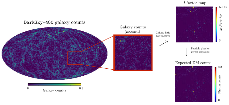
4.2.2 Dark Matter Annihilation Flux Map
One can predict the DM annihilation flux associated with a halo that surrounds a given galaxy group. This requires knowing the halo’s properties, including its mass and concentration. In this subsection, we discuss how to determine the flux when the halo’s properties are known exactly. Then, in the following subsection, we consider how to generalize the results to the more realistic scenario where the halo properties have to be inferred.
Each halo in DarkSky is fit by the Rockstar halo finder with a Navarro-Frenk-White (NFW) distribution [304] of the form
| (4.1) |
where is the scale radius and is the normalization. The NFW parameters are determined from the parameters that are provided for each DM halo—specifically, its redshift , virial mass , virial radius , and virial concentration parameter .
In the simplest scenarios, the annihilation flux factorizes as
| (4.2) |
where is the photon energy and () encodes the particle physics (astrophysical) dependence. The particle physics contribution is given by
| (4.3) |
where is the DM mass, is its annihilation cross section, is its branching fraction to the annihilation channel, is the photon energy distribution in this channel, which is modeled using PPPC4DMID [88], and is the redshift. We consider the case of annihilation into the channel as a generic example of a continuum spectrum. Of course, the exact limits will vary for different spectra, and one should consider a range of final states when applying the method to data, or use model independent-approaches (see, e.g., Ref. [305, 306]).
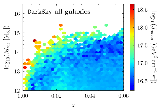
The -factor is defined as the integral along the line-of-sight of the squared DM density of the observed object:†††As defined, the -factor has units of []. This definition is convenient for extragalactic objects, but beware because another common definition of the -factor involves dividing out by a solid angle to remove the units of . A detailed discussion of the units is provided in Appendix A.
| (4.4) |
where is the line-of-sight distance and is the so-called boost factor. The boost factor accounts for the enhancement in the flux due to the annihilation in DM substructure (subhalos, subhalos within subhalos and so on…), and is usually the dominant source of systematic uncertainty in extragalactic DM annihilation studies. For the case of extragalactic objects, one can obtain a closed form solution that is an excellent approximation to the integral in Eq. 4.4, which is proportional to
| (4.5) |
where is the comoving distance (a function of redshift, ), is the critical density, and is the concentration. In our analysis, we calculate the -factor exactly, but the scaling illustrated in Eq. 4.5 is useful for understanding the dependence of on the halo mass and concentration. The derivation of the -factor expression is reviewed in detail in Appendix A, where we also show the result for the Burkert profile.
Figure 4.1 illustrates the truth -factor map associated with DarkSky, obtained by putting the observer in the center of the simulation box. This map is constructed by applying Eq. 4.4 to all host halos in the DarkSky catalog and using the boost model from Ref. [307] to describe the contribution from substructure. Once the -factors are known, the expected photon counts per pixel can be determined using Eq. 4.2 and Fermi’s exposure map. This is also shown in Fig. 4.1, assuming a DM particle with GeV that annihilates to with cms-1. Not all the pixels that contain one or more galaxies correspond to significant regions of DM annihilation. The DM annihilation flux is largest for the most massive, concentrated, and/or closest galaxy groups.
Note that when constructing Fig. 4.1, we perform the angular integrals in Eq. 4.4 as a function of angular extent, . In doing so, we implicitly assume that the boost factor is simply a multiplicative factor. In reality, the boost factor likely broadens the angular profile, because the subhalo annihilation should extend further away from the halo center. However, since the angular extent of the annihilation in most halos is small compared to the instrument point-spread function (PSF), we do not model this extension here. Some nearby halos may have significantly larger angular extent, as would be expected for the Andromeda galaxy. Nevertheless, such considerations need to be made case by case and are discussed in detail in the next chapter, where we choose to exclude Andromeda due to its size.
Figure 4.2 is a heatmap representing the average -factor, for a given and , of the DarkSky halos in the above configuration. The halos span a wide range of masses and redshifts, with -factors averaging over several orders of magnitude from 10. The largest -factors are observed for the most massive, cluster-sized halos at 0.01–0.02, as well as for less-massive halos at smaller redshifts ().
4.2.3 Uncertainties in Halo Modeling
Now, we consider more carefully the systematic uncertainties associated with modeling the halo properties. A halo with an NFW density profile has a -factor dictated by its parameters as given in Eq. 4.5. In addition to the distance, the -factor also depends on the virial mass and concentration.‡‡‡Note that uncertainties on the halo redshift also feed into the -factor. However, we consider this uncertainty to be subdominant for spectroscopically determined redshifts. For nearby halos, where the relation between distance and redshift is nontrivial, the uncertainty on the distance can be noticeably larger, and as high as 5% [308]. Nonetheless, even such uncertainties are considerably smaller than those associated with the mass and concentration, and so we do not consider them. Therefore, any uncertainty in the determination of these halo properties is propagated through to the uncertainty on the DM annihilation flux. Up until now, we have taken the halo mass and concentration directly from DarkSky, but in practice these parameters need to be inferred from properties of the observed galaxy groups.
Within DarkSky, the halo mass can be inferred from the absolute luminosity of its associated galaxy group. We obtain a deterministic relation following a procedure similar to that in Ref. [309], which derived a phenomenological relation between the -band galaxy luminosity and the mass of its DM halo. The left panel of Fig. 4.3 shows the true masses for the DarkSky halos, as a function of central galaxy luminosity (green) or the total luminosity, which includes the luminosity of the satellite galaxies (red). The DarkSky catalog provides the associations for all galaxies, central and satellite, so we include all satellites that are associated to the group when calculating the total absolute luminosity. This is similar to what is done in published group catalogs [132, 133, 295], where they account for the loss in luminosity of satellite galaxies that are farther away.
From Fig. 4.3, we see that the spread in the associated halo mass increases above L⊙, up to the brightest galaxy at L⊙, when the central galaxy luminosity is used. In contrast, the spread is significantly smaller when the total luminosity is used, making it a better predictor for the halo mass. As demonstrated in the right panel of Fig. 4.3, including the satellite luminosities allows one to better reconstruct the halo mass. Therefore, we use the median relation thus obtained as our fiducial case to infer the central mass estimate, and we use the spread in the relation to infer the uncertainty on the mass. Note that the relation shown in Fig. 4.3 is constructed by binning the DarkSky data in luminosity and calculating the 16, 50, and 84 percentiles in ; different results would be obtained by binning in and then constructing the percentiles from the luminosity distributions. This procedure is similar to that adopted by galaxy group catalogs to infer the halo mass [132, 295, 133]. Using this relation, we can infer the halo mass and uncertainty for each galaxy-group host halo in DarkSky.
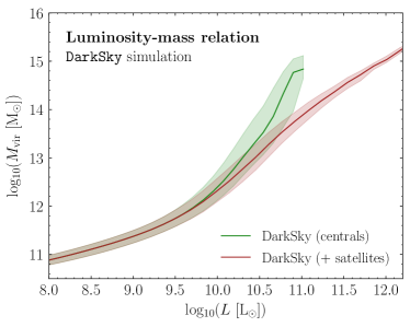
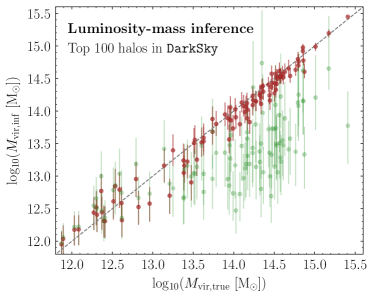
DM halos of the same mass can have very different characteristics, usually reflecting their distinct formation history and environment. One such characteristic is the halo’s virial concentration . The scale radius is the relevant quantity to compare to as it indicates an isothermal slope for the density profile, which is required for a flat rotation curve. The virial radius corresponds to the spherical volume within which the mean density is times the critical density of the Universe at that redshift. We use with in accordance with Ref. [310]. The cosmology associated with the DarkSky simulation is used throughout, with , and .
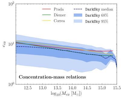
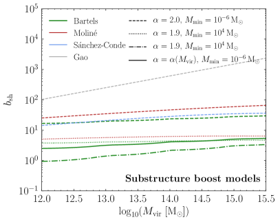
In general, the concentration correlates strongly with halo mass due to the dependence of halo formation time on mass—on average, lower mass halos tend to be more concentrated because they collapsed earlier, when the Universe was denser. For the same reason, the concentration is sensitive to the cosmology, which determines how early halos start to assemble. The concentration of field halos has been extensively studied and several concentration-mass relations have been proposed in the literature, usually based on -body simulations or physically motivated analytic approaches [316, 313, 139, 312, 311, 314, 317, 318]. In the left panel of Fig. 4.4, we show the median value of the concentration-mass relation derived directly from the DarkSky simulation, as well as the middle 68 and 95% spread. The middle 68% scatter in the relation is typically in the range 0.14-0.19 across the halo mass range considered. For comparison, we also show several concentration models that are commonly used in the literature. As is standard in the literature [110, 139], we model the uncertainty in the concentration, for a given virial mass, as a log-normal distribution around its median value.
To summarize, it is possible to infer the halo mass from the luminosity of the galaxy group and to then obtain the concentration. The final remaining property that is needed to solve for the -factor in Eq. 4.4 is the boost factor, which depends on the distribution and minimum cutoff of the subhalos’ mass. The boost factor encapsulates the complicated dependence of the subhalo mass distribution on both the particle physics assumptions of the DM model as well as the dynamics of the host halo formation. A variety of different boost models typically used in the literature are illustrated in the right panel of Fig. 4.4. As our fiducial case, we adopt the boost model of Ref. [307] (labeled as ‘Bartels Boost Model’), which self-consistently accounts for the concentration-mass relation of subhalos (compared to field halos) as well as the effects of tidal stripping. Specifically, in the subhalo mass function , we use a minimum subhalo mass cutoff of M⊙ and slope that varies self-consistently with host halo mass while accounting for evolution effects (see Ref. [307] for details).
We have now built up a framework that allows us to determine the expected DM annihilation flux map associated with a catalog of galaxy groups. Next, we show how to use this information to search for signals of DM from hundreds of galaxy groups.
4.3 Statistical Methods
In this work, we introduce and study a statistical procedure to search for gamma-ray signals from DM by stacking galaxy groups. All analyses discussed here are run on mock data, which is based on the expected astrophysical contributions to the real Fermi data set. When building this mock data set, we include contributions from (1) the diffuse emission, for which we use the Fermi Collaboration’s p7v6 model; (2) isotropic emission; (3) emission from the Fermi Bubbles [140]; and (4) emission from point sources in the Fermi 3FGL catalog [115]. The overall flux normalization for each component must be known a priori to create the mock data. To obtain this, we fit spatial maps of (1)–(4) above to the actual Fermi data. We use 413 weeks of UltracleanVeto (all PSF quartile) Pass 8 data collected between August 4, 2008 and July 7, 2016. We break the data into 40 equally log-spaced energy bins between 200 MeV and 2 TeV, applying the recommended data cuts: zenith angle , DATA_QUAL , and LAT_CONFIG . To minimize the Galactic contamination in this initial fit, we mask the region as well as the 68% containment radius for the 300 brightest and most variable sources in the 3FGL catalog. We emphasize that these masks are only used when creating the mock data and not in the stacked analysis. The fitting procedure described here provides the expected astrophysical background contribution from the real data. Monte Carlo (MC) is then generated by summing up these contributions and taking a Poisson draw from the resulting map. In the following discussion, we will show how results vary over different MC realizations of the mock data as a demonstration of Poisson fluctuations in the photon distribution.
We now describe in detail the statistical procedure we employ to implement the stacking analysis on the mock data. We perform a template-fitting profile likelihood analysis in a 10∘ region-of-interest (ROI) around each group. Template studies amount to describing the sky by a series of spatial maps (called templates). The normalization of each template is proportional to its relative gamma-ray flux. We use five templates in our study. The first four are associated with the known astrophysical sources (1)–(4) described above. Within of the halo center, we independently float the normalization of each 3FGL source.§§§The results do not change when floating all the point sources together as one combined template. This can potentially cause problems when implemented on data, however, because the 3FGL normalizations can be erroneous in certain energy bins. Allowing the normalizations of the sources to float separately helps to mitigate this potential problem. Sources outside this region may potentially contribute within the ROI because of the tails of the Fermi PSF. Therefore, between 10∘ and 18∘ of the halo center, we float the sources as a single template. The fifth and final template that we include is associated with the expected DM annihilation flux for the halo, which is effectively a map of the -factor and is described in Sec. 4.2. Note that all templates have been carefully smoothed using the Fermi PSF. The diffuse model is smoothed with the Fermi Science Tools, whereas other templates are smoothed according to the instrument response function using custom routines. Mismodeling the smoothing of either the point sources or individual halos can potentially impact the results.
A given mock data set, , is divided into 40 log-spaced energy bins indexed by . Each energy bin is then spatially binned using HEALPix [186] with nside=128 and individual pixels indexed by . In this way, the full data set is reduced to a two-dimensional array of integers describing the number of photons in energy bin and pixel . For a given halo, indexed by , only a subset of all the pixels in its vicinity are relevant. In particular, the relevant pixels are those with centers within 10∘ of the object. Restricting to these pixels leaves a subset of the data, which we denote by . Template fitting dictates that this data is described with a set of spatial templates binned in the same way as the data, which we label as , where indexes the different templates considered. The number of counts in a given pixel, energy bin, and region consists of a combination of these templates:
| (4.6) |
Here, represents the set of model parameters. For Poissonian template fitting, these are given by the normalizations of the templates , i.e., . Note that the template normalizations have an energy but not a spatial index, as the templates have an independent degree of freedom in each energy bin as written, but the spatial distribution of the model is fixed by the shapes of the templates themselves. In principle, we could also remove this freedom in the relative emission across energy bins, because we have models for the spectra of the various background components, and in particular DM. Nevertheless, we still allow the template normalizations to float independently in each energy bin for the various backgrounds. This is more conservative than assuming a model for the background spectra, and in particular we can use the shape of the derived spectra as a check that the dominant background components are being correctly modeled. The spectral shape of the DM forms part of our model prediction, however, and once we pick a final state such as annihilation to two -quarks, we fix the relative emission between the energy bins.
As we assume that the data comes from a Poisson draw of the model, the appropriate likelihood in energy bin and ROI is
| (4.7) |
Of the templates that enter this likelihood, there are some we are more interested in than others. In particular, we care about the the DM annihilation intensity, which we denote as . We treat the normalizations of the templates associated with the known astrophysical emission as nuisance parameters, . Below, we will describe how to remove the nuisance parameters to reduce Eq. 4.7 to a likelihood profile that depends only on the DM annihilation intensity, but for now we have .
Importantly, the nuisance parameters have different values between ROIs, but the DM parameters do not. This is because the DM parameters, such as the DM mass, annihilation rate, and set of final states, are universal, while the parameters that describe the astrophysical emission can vary from region to region. We do, however, profile over the -factor uncertainty in each ROI. Explicitly, each halo is given a model parameter , which is described by a log-normal distribution around the central value with width , both of which depend on the object and hence ROI considered. The -factor error, , is determined by propagating the errors associated with the mass and concentration of a given halo. To account for this, we append the following addition onto our likelihood as follows:
| (4.8) | ||||
Note that this procedure does not account for any systematic uncertainties that can bias the determination of the -factor.
The nuisance parameter can now be eliminated via the profile likelihood—see Ref. [319] for a review. Unlike for the other nuisance parameters, the value of does not depend on energy and so we eliminate the energy-dependent parameters first:
| (4.9) |
The full implementation of the profile likelihood method as suggested by this equation requires determining the maximum likelihood for the template coefficients, for every value of . Nevertheless, an excellent approximation to the profile likelihood, which is computationally more tractable, is simply to set the nuisance parameters to their maximum value obtained in an initial scan where all templates are floated.¶¶¶The DM template is only included for energy bins above 1 GeV. At lower energies, the large Fermi PSF leads to confusion between the DM, isotropic and point source templates, which can introduce a spurious preference for the DM template.
Using this approach to determine the likelihood in Eq. 4.9, we can build a total likelihood by combining the energy bins. Once this is done, the likelihood depends on the full set of DM intensities , which are specified by a DM model , cross section , mass , and -factor via Eq. 4.2. Explicitly:
| (4.10) |
and recall that unlike the other parameters on the left hand side, the -factor not only determines the , but also enters the likelihood through the expression in Eq. 4.8. We emphasize that in this equation, the DM model and mass specify the spectra, and thereby the relative weightings of the , whereas the cross section and -factor set the overall scale of the emission.
The remaining step to get the complete likelihood for a given halo is to remove , again using profile-likelihood:
| (4.11) |
This provides the full likelihood for this object as a function of the DM model parameters. The likelihood for the full stacked catalog is then simply a product over the individual likelihoods:
| (4.12) |
Using this likelihood, we define a test statistic (TS) profile as follows:
| (4.13) | ||||
where is the cross section that maximizes the likelihood for that DM model and mass. From here, we can use this TS, which is always nonpositive by definition, to set a threshold for limits on the cross-section. When searching for evidence for a signal, we use an alternate definition of the test statistic defined as
| (4.14) |
4.4 Analysis Results
In this Section, we present the results of our analysis on mock data using the DarkSky galaxy catalog. We begin by describing the sensitivity estimates associated with this study, commenting on the impact of statistical as well as systematic uncertainties and studying the effect of stacking a progressively larger number of halos. Then, we justify the halo selection criteria that are used by showing that we can recover injected signals on mock data.
4.4.1 Halo Selection and Limits
We now discuss the results obtained by applying the halo inference pipeline described in Sec. 4.2 and the statistical analysis described in Sec. 4.3 to mock gamma-ray data. We focus on the top 1000 galaxy groups in the DarkSky catalog, as ranked by the inferred -factors of their associated halos, placing ourselves at the center of the simulation box. In addition, we mask regions of the sky associated with seven large-scale structures that are challenging to model accurately: the Large and Small Magellanic Clouds, the Orion molecular clouds, the galaxy NGC5090, the blazar 3C454.3, and the pulsars J1836+5925 and Geminga. This is done here for simulated data in order to closely track the analysis that will subsequently be performed on real Fermi data.
While we start from an initial list of 1000 galaxy groups, we do not include all of them in the stacking procedure. A galaxy group is excluded if:
-
1.
it is located within ;
-
2.
it is located less than from the center of another brighter group in the catalog;
-
3.
it has TS and ,
where is the best-fit cross section at any mass and is the best-fit limit set by any halo at the specified DM mass. Note that the second requirement is applied sequentially to the ranked list of halos, ordered by -factor. We now explain the motivation for each of these requirements separately. The first requirement listed above removes groups that are located close to the Galactic plane to reduce contamination from regions of high diffuse emission and the associated uncertainties in modeling these. The second requirement demands that the halos be reasonably well-separated, which avoids issues having to do with overlapping halos and accounting for multiple DM parameters in the same ROI. The non-overlap criterion of 2∘ is chosen based on the Fermi PSF containment in the lowest energy bins used and on the largest spatial extent of gamma-ray emission associated with the extended halos, which collectively drive the possible overlap between nearby halos.
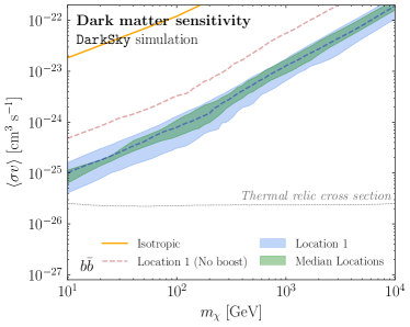
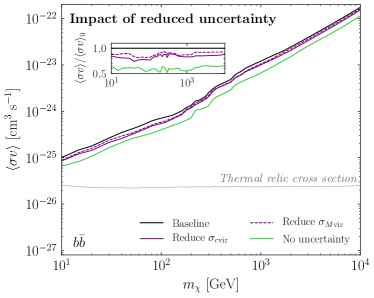
The final requirement excludes a galaxy group if it has an excess of at least 3 significance associated with the DM template that is simultaneously excluded by the other galaxy groups in the sample. This selection is necessary because we expect that some galaxy groups will have true cosmic-ray-induced gamma-ray emission from conventional astrophysics in the real data, unrelated to DM. To identify these groups, we take advantage of the fact that we are starting from a large population of halos that are all expected to be bright DM sources in the presence of a signal. Thus, if one halo sets a strong limit on the annihilation rate and another halo, at the same time, has a large excess that is severely in conflict with the limit, then most likely the large excess is not due to DM. The worry here is that we could have mis-constructed the -factor of the halo that gave the strong limit, so that the real limit is not as strong as we think it is. However, with the TS and criteria outlined above, this does not appear to be the case. In particular, we find that the criteria very rarely rejects halos due to statistical fluctuations. For example, over 50 MC iterations of the mock data, halos (out of 1000) remain after applying the TS and cross section cuts alone, and the excluded halos tend to have lower -factors, since there the requirement is more readily satisfied.
We expect that this selection criteria will be very important on real data, however, where real excesses can abound. In addition, as we will describe in the next subsection, injected signals are not excluded when the analysis pipeline is run on mock data. In an ideal scenario, we would attempt to understand the origin of these excesses by correlating their emission to known astrophysics either individually or statistically. In the present analysis, however, we take the conservative approach of removing halos that are robustly inconsistent with a DM signal and leave a deeper understanding of the underlying astrophysics to future work.
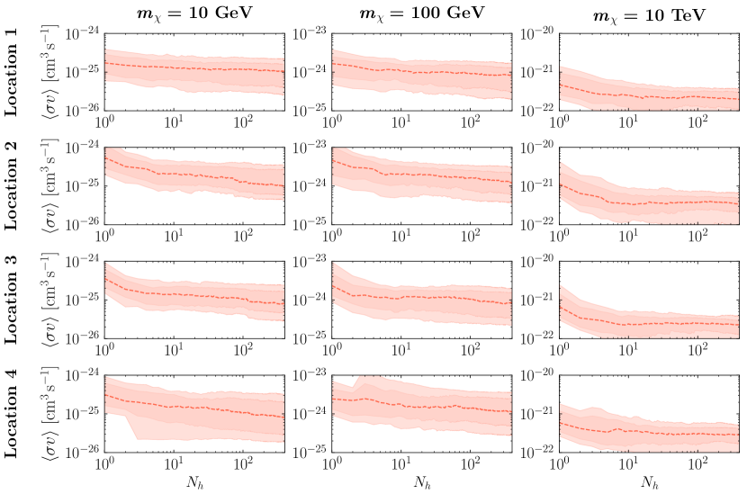
We apply the procedure outlined in Secs. 4.2 and 4.3 to the mock data to infer the 95% confidence limit on the DM annihilation cross section. The resulting sensitivity is shown by the blue dashed line in the left panel of Fig. 4.5, which uses the boost factor from Ref. [307]. For comparison, we also show the limit assuming no boost factor (red dashed line); note that the boost factor model that we use provides a modest improvement to the limit. Because the limit can potentially vary over different MC realizations of the mock data, we repeat the procedure for 100 MCs (associated with different Poisson realizations of the map); the blue band indicates the middle 68% spread in the limit associated with this statistical variation.
To see how the limit depends on the observer’s location within the DarkSky simulation box, we repeat the procedure described above over nine different locations.∥∥∥The nine locations we used are at the following coordinates Mpc/h in DarkSky: , , , , , , , , . The first listed location is our default position, and any time we use more than one location they are selected in order from this list. At each location, we perform 20 MCs and obtain the median DM limit. The green band in the left panel of Fig. 4.5 denotes the middle 68% spread on the median bounds for each of the different sky locations. In general, we find that the results obtained by an observer at the center of the DarkSky box are fairly representative, compared to random locations. Note, however, that this bound does not necessarily reflect the sensitivity reach one would expect to get with actual Fermi data. The reason for this is that the locations probed in DarkSky do not resemble that of the Local Group in detail. We will come back to this point below, when we compare the -factors of the DarkSky halos to those from galaxy catalogs that map the local Universe.
The orange line in the left panel of Fig. 4.5 shows the limit obtained by requiring that the DM emission from the groups not overproduce the measured isotropic gamma-ray component [199]. This should not be compared to the published DM bounds obtained with the Fermi Isotropic Gamma-Ray Background [117] because that study accounts for the integrated effect of the DM annihilation flux from halos much deeper than those we consider here. The inclusion of these halos results in a total flux that can be greater than those from our sample by over an order of magnitude. Nevertheless, this gives an idea of how much we gain by resolving the spatial structure of the local DM population and knowing the locations of the individual galaxy groups.
The right panel of Fig. 4.5 shows the effect of propagating uncertainties associated with inferring the halo properties. The green line indicates how the limit improves when no uncertainties are assumed, i.e., we can perfectly reconstruct the virial mass and concentration of the halos. The sensitivity reach improves by roughly a factor of two in this case. We further show the effect of individually reducing the error on (dashed purple line) and (purple line) by 50%. The reductions in the uncertainties provide only marginal improvements to the overall sensitivity, still far below the level of systematic uncertainty associated with extragalactic analyses in general.
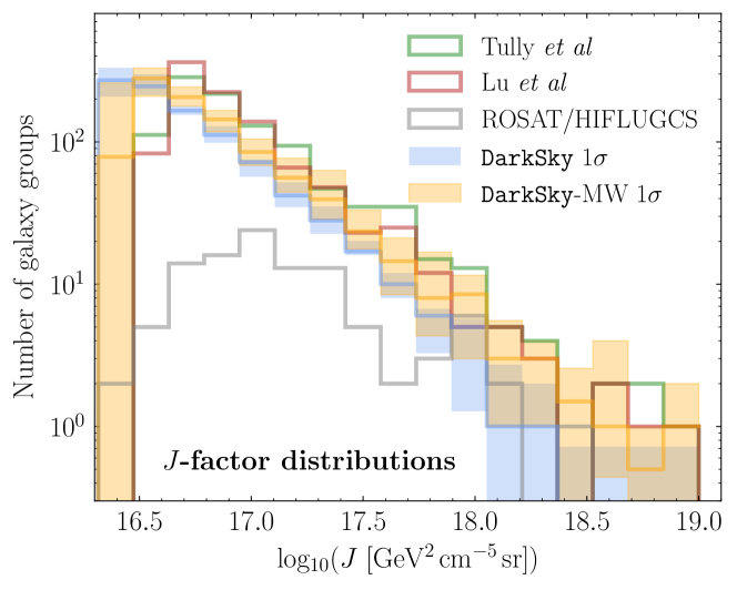
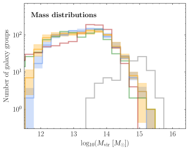
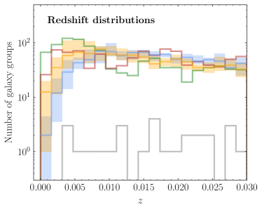
It is interesting to study how the limit scales with the number of halos, , included in the stacking procedure. This result is shown in Fig. 4.6 for and GeV, for four different observer locations in the simulation box. The dashed red line indicates the median 95% confidence limit. The red bands are the 2.5, 16, 84 and 97.5 percentiles on the limit, obtained from 100 MC realizations of the mock data. We observe that the limit typically improves continuously for the first 10 halos. As more halos are included in the stacking, the gains diminish. For some sky locations, the limit simply remains flat; for others we see some marginal improvements in the bounds. These results are consistent, within uncertainties, between the DM masses and the different sky locations of the observer.
We emphasize that the scaling on can be very different on applicaton to real data, because the distribution of -factors in the random DarkSky locations is not representative of our own environment in the Local Group and also some halos can have residuals that are not related to DM but rather to mismodeling or real cosmic-ray–induced emission from the galaxy groups. The former point is demonstrated in Fig. 4.7, where we histogram the top 1000 -factors associated with the baseline DarkSky analysis (blue line/band). For comparison, we also show the distributions corresponding to 2MRS galaxy group catalogs, specifically the Tully et al. [132, 133] (green line) and the Lu et al. [295] (red line) catalogs. We see that the distribution of -factors for the 2MRS catalogs is skewed towards higher values compared to that from DarkSky. (Note that the cut-off at low -factors is artificial and is simply a result of including 1000 halos for each catalog.)
The differences in the -factor distributions can be traced to the redshift distribution of the galaxy groups, as illustrated in Fig. 4.8. We see specifically that the mass function of the top 1000 DarkSky halos in each of the random sky locations sampled is roughly consistent with that observed in the 2MRS catalogs. In contrast, the actual catalogs have more groups at lower than observed in the random DarkSky locations.
While a random location in the DarkSky box does not resemble our own Local Group, we can try to find specific locations in the simulation box that do. Therefore, we place the observer at ten random Milky Way–like halos in the simulation box, which have a mass M⊙. More specifically, we select halos with mass and at least 100 Mpc from the box boundaries. The distribution of the top 1000 -factors is indicated by the orange line/band in Fig. 4.7, while the corresponding mass and redshift distributions are shown in Fig. 4.8. We see that the redshift—and, consequently, -factor—distributions approach the observations, though the correspondence is still not exact. A more thorough study could be done assessing the likelihood that an observer in DarkSky is located at a position that closely resembles the Local Group. However, as our primary goal here is to outline an analysis procedure that we can apply to actual data, we simply conclude that our own local Universe appears to be a richer environment compared to a random location within the DarkSky simulation box, which bodes well for studying the actual Fermi data.
4.4.2 Signal Recovery Tests
It is critical that the halo selection criteria described in the previous section do not exclude a potential DM signal if one were present. To verify this, we have conducted extensive tests where we inject a signal into the mock data, pass it through the analysis pipeline and test our ability to accurately recover its cross section in the presence of the selection cuts. Figure 4.9 summarizes the results of the signal injection tests for two different observer locations in the DarkSky simulation box (top and bottom rows, respectively). We inject a signal in the mock data that is associated with annihilation for three different masses ( GeV) that traces the DM annihilation flux map associated with DarkSky. The dashed line in each panel delineates where the injected cross section, , matches the recovered cross section, .
The green line shows the 95% one-sided limit on the cross section found using Eq. 4.13, with a TS threshold corresponding to . The green band shows the 68% containment region on this limit, constructed from twenty different MC realizations of the mock data set. Importantly, the limit on roughly follows—but is slightly weaker than—the injected signal, up until the maximum sensitivity is reached and smaller cross sections can no longer be probed. This behavior is generally consistent between the three DM masses tested and both sky locations. We clearly see that the limit obtained by the statistical procedure never excludes an injected signal over the entire cross section range.
Next, we consider the recovered cross section that is associated with the maximum test statistic, TS, in the total likelihood. The blue line in each panel of Fig. 4.9 shows the median value of over 20 MCs of the mock data. The blue band spans the median cross sections associated with . The inset show the median and 68% containment region for TS as a function of the injected cross section. The maximum test statistic is an indicator for the significance of the DM model and as such the distributions are only influenced by the data at high injected cross sections where TS has begun to increase. At lower injected cross sections, the distributions for are not meaningful.
Two issues are visible in Fig. 4.9: (i) at high injected cross sections, the best-fit recovered cross sections are systematically around 1 too high, and (ii) at high DM masses and near-zero injected cross sections, the distribution of TS deviates from the chi-square distribution (which can be seen based on the fact that the TS flattens out with a non-zero median value). The first issue stems from the way we model the -factor contribution to the likelihood, while the second arises from the approximations we make to perform the profile likelihood in a computationally efficient manner.
4.5 Conclusions
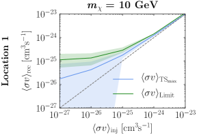

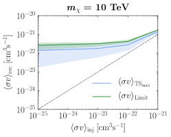
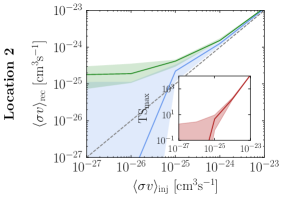
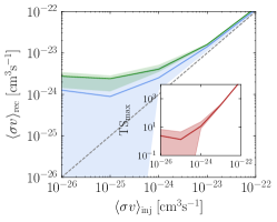
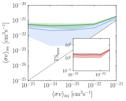
In this chapter, we introduced a procedure to build a full-sky map of extragalactic DM targets based on galaxy surveys and demonstrated this methodology using the DarkSky cosmological simulation. Starting from the galaxies in the DarkSky catalog, we inferred the properties of their respective DM halos using the galaxy-halo connection. In so doing, we identified the halos that are the brightest sources of extragalactic DM annihilation and which act as the best annihilation targets. This procedure allows us to account for the fact that not all galaxy groups are expected to be bright DM emitters; the most massive, concentrated, and/or most nearby galaxies dominate the signals. By building a map of extragalactic DM targets, we can focus our search for DM annihilation on the most relevant regions of sky. This philosophy contrasts with that of cross-correlation studies, which treat all galaxies as equally good targets for DM.
With a list of extragalactic DM halos in hand, as well as their inferred -factors, we performed a stacked analysis to search for gamma-ray signatures of DM annihilation in mock data. We described the likelihood procedure for the stacking analysis in detail. There are two clear advantages to this approach over, say, a full-sky template study. First, focusing on smaller regions around each halo significantly reduces the sensitivity to mis-modeling of the foregrounds. Second, uncertainties on the predicted DM annihilation flux can be straightforwardly included in the likelihood function. In particular, we outlined how uncertainties in the -factors, which arise from the determination of the virial mass and concentration, are marginalized over in the analysis.
We presented limits on the DM annihilation cross section for mock data and, most importantly, demonstrated that the analysis procedure robustly recovers injected signals. We found that the sensitivity improves by nearly two orders of magnitude when the structure of extragalactic DM emission on the sky is accounted for, rather than simply assuming an isotropic distribution. Typically, the limit is dominated by the brightest halos in the stacking, though this varies depending on the location in the simulation box. The -factor distribution of nearby groups in our own Galaxy differs from the random locations sampled in the DarkSky box, which can change the number of halos that dominate the limit. In actuality, one would want to continue adding halos to the analysis—ranked starting from the brightest -factors—until the gains in the limit are observed to level off.
One advantage of using the DarkSky simulation in this initial study is that the truth information for all the halos is known. We can therefore study how the DM limits improve when the virial mass and concentration of the halos are known precisely. For this ideal scenario, we find that that the limits improve by roughly 50% over those obtained by marginalizing over uncertainties. This suggests that a concrete way to improve the bounds on DM annihilation is to reduce the uncertainties on and for the brightest halos in the catalog.
The substructure boost factor remains one of the most difficult systematics to handle. In this work, we use recent boost factor models that account for tidal stripping of subhalos. This boost factor changes the limit by an factor, which is more conservative than other models sometimes used in extragalactic DM studies. While the boost factor enhancement is fairly modest, it is still the dominant systematic uncertainty over the halo mass and concentration.
The analysis outlined in this chapter can be repeated on Fermi data using published galaxy group catalogs. In particular, the Tully et al. catalogs [132, 133] and the Lu et al. catalog [295] provide a map of the galaxy groups in the local Universe within . Both catalogs are based primarily on 2MRS, but use different clustering algorithms and halo mass determinations. Taken together, they provide a way to estimate the systematic uncertainties associated with the galaxy to halo mapping procedure. Previous cluster studies on Fermi data [287, 288, 289, 290, 293] used the extended HIghest X-ray FLUx Galaxy Cluster Sample (HIFLUGCS) [322, 323], which includes 106 of the brightest clusters observed in X-ray with the ROSAT all-sky survey. These clusters cover redshifts from ; the distribution of their -factors, masses, and redshifts are shown in Fig. 4.7 and 4.8. In general, the 2MRS catalogs provide a larger number of groups that should be brighter in DM annihilation flux, so we expect a corresponding improvement in the sensitivity to annihilation signatures.
The recent advancement of galaxy catalogs based on 2MRS and other nearby group catalogs allows us for the first time to map out the most important extragalactic DM targets in the nearby Universe. This, in turn, enables us to perform a search that focuses on regions of sky where we expect the DM signals to be the brightest outside the Local Group. We present the complete results of such an analysis, as applied to data, in the next chapter.
Chapter 5 A Search for Dark Matter Annihilation in Galaxy Groups
This chapter is based on an edited version of A Search for Dark Matter Annihilation in Galaxy Groups, Phys.Rev.Lett. 120 (2018) 101101 [arXiv:1708.09385] with Mariangela Lisanti, Nicholas Rodd and Benjamin Safdi [134]. The results of this chapter have been presented at the following conferences and workshops: TeV Particle Astrophysics (TeVPA) 2017 in Columbus, OH (August 2017), Dark Matter, Neutrinos and their Connection (DACO) in Odense, Denmark (August 2017), Workshop on Statistical Challenges in the Search for Dark Matter in Banff, Canada (February 2018) and Recontres de Blois 2018 in Blois, France (June 2018).
5.1 Introduction
Weakly-interacting massive particles, which acquire their cosmological abundance through thermal freeze-out in the early Universe, are leading candidates for dark matter (DM). Such particles can annihilate into Standard Model states in the late Universe, leading to striking gamma-ray signatures that can be detected with observatories such as the Fermi Large Area Telescope. Some of the strongest limits on the annihilation cross section have been set by searching for excess gamma-rays in the Milky Way’s dwarf spheroidal satellite galaxies (dSphs) [90, 89]. In this chapter, we present competitive constraints that are obtained using hundreds of galaxy groups within .
Chapter 4 describes the procedure for utilizing galaxy group catalogs in searches for extragalactic DM. Previous attempts to search for DM outside the Local Group were broad in scope, but yielded weaker constraints than the dSph studies. For example, limits on the annihilation rate were set by requiring that the DM-induced flux not overproduce the isotropic gamma-ray background [117]. These bounds could be improved by further resolving the contribution of sub-threshold point sources to the isotropic background [164, 165], or by looking at the auto-correlation spectrum [276, 276, 278, 279]. A separate approach involves cross-correlating [281, 122, 121, 126, 125, 124, 123] the Fermi data with galaxy-count maps constructed from, e.g., the Two Micron All-Sky Survey (2MASS) [324, 299]. A positive cross-correlation was detected with 2MASS galaxy counts [126], which could arise from annihilating DM with mass – GeV and a near-thermal annihilation rate [125]. However, other source classes, such as misaligned Active Galactic Nuclei, could also explain the signal [124].
| Name | ||||||||
| [GeV2 cm-5 sr] | [] | [deg] | [deg] | [deg] | ||||
| NGC4472/Virgo | 19.110.35 | 14.60.14 | 3.58 | 283.94 | 74.52 | 0.800.18 | 1.15 | 4.53 |
| NGC0253 | 18.760.37 | 12.70.12 | 0.79 | 98.24 | -87.89 | 1.000.17 | 0.77 | 2.90 |
| NGC3031 | 18.580.36 | 12.60.12 | 0.83 | 141.88 | 40.87 | 1.020.17 | 0.64 | 2.76 |
| NGC4696/Cen. | 18.330.35 | 14.60.14 | 8.44 | 302.22 | 21.65 | 0.800.18 | 0.47 | 4.50 |
| NGC1399 | 18.300.37 | 13.80.13 | 4.11 | 236.62 | -53.88 | 0.890.17 | 0.45 | 3.87 |
An alternative to studying the full-sky imprint of extragalactic DM annihilation is to use individual galaxy clusters [287, 288, 289, 116, 290, 291, 292, 293, 296, 325]. Previous analyses along these lines have looked at a small number of – M⊙ clusters whose properties were inferred from X-ray measurements [322, 323]. Like the dSph searches, the cluster studies have the advantage that the expected signal is localized in the sky, which reduces the systematic uncertainties associated with modeling the foregrounds and unresolved extragalactic sources. As we will show, however, the sensitivity to DM annihilation is enhanced—and is more robust—when a larger number of targets are included compared to previous studies.
Our work aims to combine the best attributes of the cross-correlation and cluster studies to improve the search for extragalactic DM annihilation. We use the galaxy group catalogs in Refs. [132] and [133] (hereby T15 and T17, respectively), which contain accurate mass estimates for halos with mass greater than M⊙ and , to systematically determine the galaxy groups that are expected to yield the best limits on the annihilation rate. The T15 catalog provides reliable redshift estimates in the range , while the T17 catalog provides measured distances for nearby galaxies, , based on Ref. [308]. The T15 catalog was previously used for a gamma-ray line search [296], but our focus here is on the broader, and more challenging, class of continuum signatures. We search for gamma-ray flux from these galaxy groups and interpret the null results as bounds on the annihilation cross section.
5.2 Galaxy Group Selection
The observed gamma-ray flux from DM annihilation in an extragalactic halo is proportional to both the particle physics properties of the DM, as well as its astrophysical distribution:
| (5.1) |
with units of . Here, is the gamma-ray energy, is the annihilation cross section, is the DM mass, is the branching fraction to the annihilation channel, and is the cosmological redshift. The energy spectrum for each channel is described the function , which is modeled using PPPC4DMID [88]. The -factor that appears in Eq. 5.1 encodes the astrophysical properties of the halo. It is proportional to the line-of-sight integral of the squared DM density distribution, , and is written in full as
| (5.2) |
where is the boost factor, which accounts for the enhancement due to substructure. For an extragalactic halo, where the comoving distance is much greater than the virial radius , the integral in Eq. 5.2 scales as for the Navarro-Frenk-White (NFW) density profile [326]. Here, is the virial mass, is the critical density, and is the virial concentration, with the scale radius. We infer using the concentration-mass relation from Ref. [311], which we update with the Planck 2015 cosmology [20]. For a given mass and redshift, the concentration is modeled as a log-normal distribution with mean given by the concentration-mass relation. We estimate the dispersion by matching to that observed in the DarkSky-400 simulation for an equivalent [298]. Typical dispersions range from – over the halo masses considered.
The halo mass and redshift also determine the boost factor enhancement that arises from annihilation in DM substructure. Accurately modeling the boost factor is challenging as it involves extrapolating the halo-mass function and concentration to masses smaller than can be resolved with current simulations. Some previous analyses of extragalactic DM annihilation have estimated boost factors – for cluster-size halos (see, for example, Ref. [315]) based on phenomenological extrapolations of the subhalo mass and concentration relations. However, more recent studies indicate that the concentration-mass relation likely flattens at low masses [327, 328, 311], suppressing the enhancement. We use the model of Ref. [307]—specifically, the “self-consistent” model with M⊙—which accounts for tidal stripping of bound subhalos and yields a modest boost for M⊙ halos. Additionally, we model the boost factor as a multiplicative enhancement to the rate in our main analysis, though we consider the effect of possible spatial extension from the subhalo annihilation in App. B. In particular, we find that modeling the boost component of the signal as tracing a subhalo population distributed as rather than degrades the upper limits obtained by almost an order of magnitude at higher masses GeV while strengthening the limit by a small factor at lower masses GeV. This is arguably a more plausible scenario, since the spatial distribution of subhalos is expected to follow the overall shape of the dark matter halo rather than the annihilation profile (modulo baryonic effects).
The halo masses and redshifts are taken from the galaxy group catalog T15 [132], which is based on the 2MASS Redshift Survey (2MRS) [329], and T17 [133], which compiles an inventory of nearby galaxies and distances from several sources. The catalogs provide group associations for these galaxies as well as mass estimates and uncertainties of the host halos, constructed from a luminosity-to-mass relation. The mass distribution is assumed to follow a log-normal distribution with uncertainty fixed at 1% in log-space (see Ch. 4), which translates to typical absolute uncertainties of 25-40%.***To translate, approximately, between log- and linear-space uncertainties for the mass, we may write , which implies that the linear-space fractional uncertainties are . This is conservative compared to the 20% uncertainty estimate given in T15 due to their inference procedure. The halo centers are assumed to coincide with the locations of the brightest galaxy in the group. We infer the -factor using Eq. 5.2 and calculate its uncertainty by propagating the errors on and , which we take to be uncorrelated. Note that we neglect the distance uncertainties, which are expected to be 5% [308, 133], as they are subdominant compared to the uncertainties on mass and concentration. We compile an initial list of nearby targets using the T17 catalog, supplementing these with the T15 catalog. We exclude from T15 all groups with Local Sheet velocity km s-1 () and km s-1 (), the former because of peculiar velocity contamination and the latter because of large uncertainties in halo mass estimation due to less luminous satellites. When groups overlap between the two catalogs, we preferentially choose distance and mass measurements from T17.
The galaxy groups are ranked by their inferred -factors, excluding any groups that lie within to mitigate contamination from Galactic diffuse emission. We require that halos do not overlap to within of each other, which is approximately the scale radius of the largest halos. The exclusion procedure is applied sequentially starting with a halo list ranked by -factor. We manually exclude Andromeda, the brightest halo in the catalog, because its large angular size is not ideally suited to our analysis pipeline and requires careful individual study [286]. As discussed later in this chapter, halos are also excluded if they show large residuals that are inconsistent with DM annihilation in the other groups in the sample. Starting with the top 1000 halos, we end up with 495 halos that pass all these requirements. Of the excluded halos, 276 are removed because they fall too close to the Galactic plane, 134 are removed by the proximity requirement, and 95 are removed because of the cut on large residuals. Other than the manual exclusion of Andromeda, these selection criteria are identical to those introduced and tested in Ch. 4 in the context of simulations.
Table 5.1 lists the top five galaxy groups included in the analysis, labeled by their central galaxy or common name, if one exists. We provide the inferred -factor including the boost factor, the halo mass, redshift, position in Galactic coordinates, inferred concentration, and boost factor. Additionally, we show to indicate the spatial extension of the halo. We find that is typically between the 68% and 95% containment radius for emission associated with annihilation in the halos, without accounting for spread from the point-spread function (PSF). For reference, Andromeda has . A complete list of the analyzed galaxy groups is provided as Supplementary Data at https://github.com/bsafdi/DMCat.
5.3 Data Analysis
We analyze 413 weeks of Pass 8 Fermi data in the UltracleanVeto event class, from August 4, 2008 through July 7, 2016. The data is binned in 26 logarithmically-spaced energy bins between 502 MeV and 251 GeV and spatially with a HEALPix pixelation [186] with nside=128.†††Our energy binning is constructed by taking 40 log-spaced bins between 200 MeV and 2 TeV and then removing the lowest four and highest ten bins, for reasons discussed in Ch. 4 The recommended set of quality cuts are applied to the data corresponding to zenith angle less than , , and .‡‡‡https://fermi.gsfc.nasa.gov/ssc/data/analysis/documentation/Cicerone/Cicerone_Data_Exploration/Data_preparation.html. We also mask known large-scale structures (see Ch. 4).
The template analysis that we perform using NPTFit [142] is similar to that of previous dSph studies [90, 89] and is detailed in Ch. 4. We summarize the relevant points here. Each region-of-interest (ROI), defined as the area surrounding each halo center, has its own likelihood. In each energy bin, this likelihood is the product, over all pixels, of the Poisson probability for the observed photon counts per pixel. This probability depends on the mean expected counts per pixel, which depends on contributions from known astrophysical emission as well as a potential DM signal. Note that the likelihood is also multiplied by the appropriate log-normal distribution for , which we treat as a single nuisance parameter for each halo and account for through the profile likelihood method.
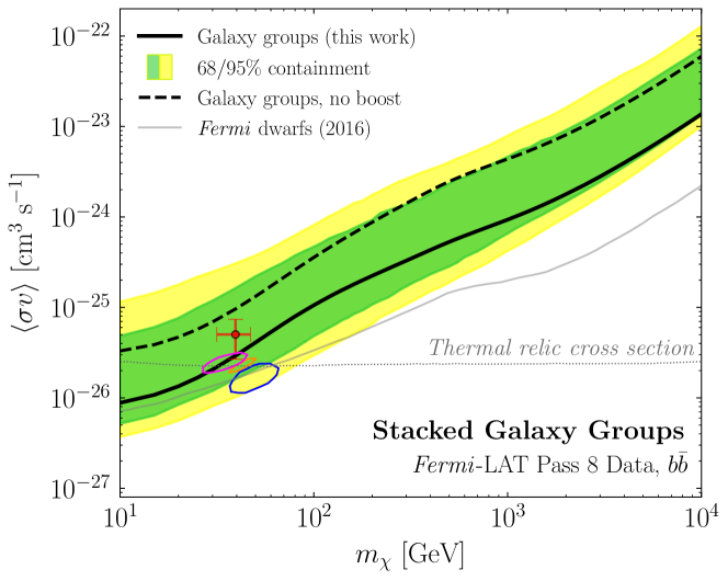
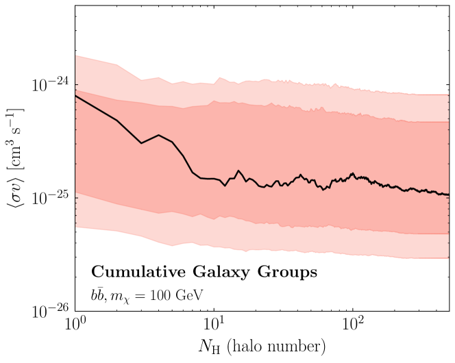
To model the expected counts per pixel, we include several templates in the analysis that trace the emission associated with: (i) the projected NFW-squared profile modeling the putative DM signal, (ii) the diffuse background, as described by the Fermi gll_iem_v06 (p8r2) model, (iii) isotropic emission, (iv) the Fermi bubbles [140], (v) 3FGL sources within to of the halo center, floated together after fixing their individual fluxes to the values predicted by the 3FGL catalog [115], and (vi) all individual 3FGL point sources within of the halo center. Note that we do not model the contributions from annihilation in the smooth Milky Way halo because the brightest groups have peak flux significantly (approximately an order of magnitude for the groups in Tab. 5.1) over the foreground emission from Galactic annihilation and because we expect Galactic annihilation to be subsumed by the isotropic component.
We assume that the best-fit normalizations (i.e., profiled values) of the astrophysical components, which we treat as nuisance parameters, do not vary appreciably with DM template normalization. This allows us to obtain the likelihood profile in a given ROI and energy bin by profiling over them in the presence of the DM template, then fixing the normalizations of the background components to the best-fit values and scanning over the DM intensity. We then obtain the total likelihood by taking the product of the individual likelihoods from each energy bin. In order to avoid degeneracies at low energies due to the large PSF, we only include the DM template when obtaining the best-fit background normalizations at energies above GeV. At the end of this procedure, the likelihood is only a function of the DM template intensity, which can then be mapped onto a mass and cross section for a given annihilation channel. We emphasize that the assumptions described above have been thoroughly vetted in Ch. 4, where we show that this procedure is robust in the presence of a potential signal.
The final step of the analysis involves stacking the likelihoods from each ROI. The stacked log-likelihood, , is simply the sum of the log-likelihoods for each ROI. It follows that the test statistic for data is defined as
| (5.3) | ||||
where is the cross section that maximizes the likelihood for DM model . The 95% upper limit on the annihilation cross section is given by the value of where .
Galaxy groups are expected to emit gamma-rays from standard cosmic-ray processes. Using group catalogs to study gamma-ray emission from cosmic rays in these objects is an interesting study in its own right (see, e.g., Ref. [330, 331, 116, 291]), which we leave to future work. For the purpose of the present analysis, however, we would like a way to remove groups with large residuals, likely arising from standard astrophysical processes in the clusters, to maintain maximum sensitivity to DM annihilation. This requires care, however, as we must guarantee that the procedure for removing halos does not remove a real signal, if one were present.
We adopt the following algorithm to remove halos with large residuals that are inconsistent with DM annihilation in the other groups in the sample. A group is excluded if it meets two conditions. First, to ensure it is a statistically significant excess, we require twice the difference between the maximum log likelihood and the log likelihood with to be greater than 9 at any DM mass. This selects sources with large residuals at a given DM mass. Second, the residuals must be strongly inconsistent with limits set by other galaxy groups. Specifically, the halo must satisfy , where is the halo’s best-fit cross section at any mass and is the strongest limit out of all halos at the specified . These conditions are designed to exclude galaxy groups where the gamma-ray emission is inconsistent with a DM origin. This prescription has been extensively tested on mock data and, crucially, does not exclude injected signals (see Ch. 4).
5.4 Results
Figure 5.1 illustrates the main results of the stacked analysis. The solid black line represents the limit obtained for DM annihilating to a final state using the fiducial boost factor model [307], while the dashed line shows the limit without the boost factor enhancement (results for final states other than are presented in App. B). To estimate the expected limit under the null hypothesis, we repeat the analysis by randomizing the locations of the halos on the sky 200 times, though still requiring they pass the selection cuts described above. The colored bands indicate the 68 and 95% containment regions for the expected limit. The limit is consistent with the expectation under the null hypothesis.
Figure 5.2 illustrates how the limits evolve for the final state with GeV as an increasing number of halos are stacked. We also show the expected 68% and 95% containment regions, which are obtained from the random sky locations. As can be seen, no single halo dominates the bounds. For example, removing Virgo, the brightest halo in the catalog, from the stacking has no significant effect on the limit. Indeed, the inclusion of all 495 halos buys one an additional order of magnitude in the sensitivity reach.
Fig. 5.3 shows a Mollweide projection of all the -factors inferred using the T15 and T17 catalogs, smoothed at with a Gaussian kernel. The map is shown in Galactic coordinates with the Galactic Center at the origin. Looking beyond astrophysical sources, this is how an extragalactic DM signal might show up in the sky. Although this map has no masks added to it, a clear extinction is still visible along the Galactic plane. This originates from the incompleteness of the catalogs along the Galactic plane.
The limit derived in this work is complementary to the published dSph bound [90, 89], shown as the solid gray line in Fig. 5.1. Given the large systematic uncertainties associated with the dwarf analyses (see e.g., Ref. [91]), we stress the importance of using complementary targets and detection strategies to probe the same region of parameter space. Our limit also probes the parameter space that may explain the Galactic Center excess (GCE); the best-fit models are marked by the orange cross [150], blue [98], red [99], and orange [95] regions. The GCE is a spherically symmetric excess of GeV gamma-rays observed to arise from the center of the Milky Way [96, 97, 100, 101]. The GCE has received a considerable amount of attention because it can be explained by annihilating DM. However, it can also be explained by more standard astrophysical sources; indeed, recent analyses have shown that the distribution of photons in this region of sky is more consistent with a population of unresolved point sources, such as millisecond pulsars, compared to smooth emission from DM [102, 103, 161, 332]. Because systematic uncertainties can be significant and hard to quantify in indirect searches for DM, it is crucial to have independent probes of the parameter space where DM can explain the GCE. While our null findings do not exclude the DM interpretation of the GCE, their consistency with the dwarf bounds (which also cut into the GCE region) put it further in tension. This does not, however, account for the fact that the systematics on the modeling of the Milky Way’s density distribution can potentially alleviate the tension by changing the best-fit cross section for the GCE.
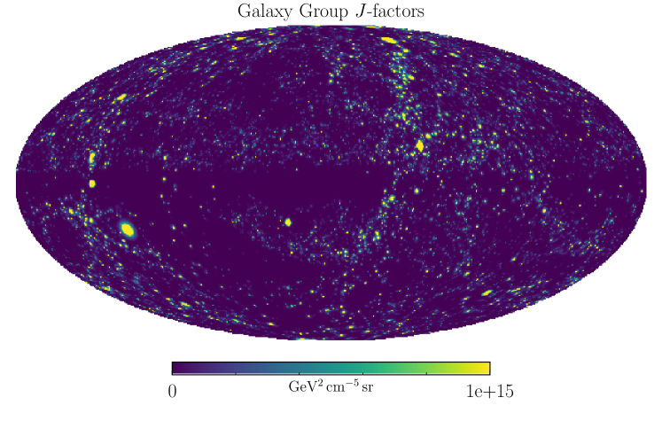
5.5 Conclusions
This chapter presents the results of the first systematic search for annihilating DM in nearby galaxy groups. We introduced and validated a prescription to infer properties of DM halos associated with these groups, thereby allowing us to build a map of DM annihilation in the local Universe. Using this map, we performed a stacked analysis of several hundred galaxy groups and obtained bounds that exclude thermal cross sections for DM annihilating to with mass below GeV, assuming a conservative boost factor model. These limits are competitive with those obtained from the Fermi dSph analyses and are in tension with the range of parameter space that can explain the GCE. Moving forward, we plan to investigate the objects with gamma-ray excesses to see if they can be interpreted in the context of astrophysical emission. In so doing, we can also develop more refined metrics for selecting the optimal galaxy groups for DM studies.
We include additional results in App. B that further extends the results presented here. There, we show limits for additional annihilation final states and the brightest individual halos. We also show how the limits are affected by several analysis choices, such as the inclusion of Andromeda and Virgo, as well as a variety of systematic uncertainties. A complete table of the galaxy groups used in this analysis, as well as their associated properties, are provided in Supplementary Data, which can be accessed at https://github.com/bsafdi/DMCat. The catalog includes decay factors for all of the groups in addition to the annihilation -factors. We emphasize that the supplementary catalog is separate from the Fermi analysis presented here and may be used to search for extragalactic DM annihilation and decay into neutral cosmic rays, regardless of wavelength, messenger, and instrument.
Appendix A - and -factors for Extragalactic Sources
In this Appendix, we derive the -factor relations used in the main text. We also derive the corresponding -factor relations, which apply to the case of decaying DM. Although we do not make use of the decay results in the main text, we include these results for completeness because much of our main analysis can be extended to the decaying case. This Appendix is broken into three subsections. In the first of these, we detail the units and conventions used in our definition of the - and -factors. After this, we derive an approximate form of the astrophysics factors for different DM density profiles and discuss the accuracy of the approximations made. We conclude with a discussion of error propagation in the -factors. Note that several of the details presented in these appendices have been discussed elsewhere, see e.g., Ref. [333, 334, 335, 336].
A.1 Units and Conventions
A.1.1 Dark Matter Flux
We begin by carefully outlining the units associated with the - and -factors. The flux, , associated with either DM annihilation or decay factorizes into two parts:
| (A.1) | ||||
where is the photon energy and the ‘ann.’ (‘dec.’) superscripts denote annihilation (decay). The particle physics factors are given by:
| (A.2) | ||||
where is the velocity-averaged annihilation cross section, is the DM mass, Bri is the branching fraction into the channel, is the photon energy distribution associated with this channel, and is the DM lifetime. The annihilation factor assumes that the DM is its own antiparticle; if this were not the case, and assuming no asymmetry in the dark sector, then the factor would be half as large. The particle physics factors carry the following dimensions:
| (A.3) | ||||
where ‘counts’ refers to the number of gamma-rays produced in the interaction and the is associated with the in the particle physics factors. Note that some references include this in the definition of the - or -factors, but this is not the convention that we follow here.
The - and -factors are defined as follows:
| (A.4) | ||||
where is the subhalo boost factor. The - and -factors carry the following units:
| (A.5) | ||||
Combining these with Eq. A.3, we find that
| (A.6) |
for both the annihilation and decay case. This means that is given in units of counts per experimental effective area [] per experimental run time []. In this work, we study extragalactic objects with small angular extent. So long as each object is centered on the region-of-interest (ROI), we expect that all of its flux will be contained within the ROI as well. This means that the photon counts obtained by integrating Eq. A.4 over the entire sky corresponds to the total counts expected from that object in the ROI. The situation is different when treating objects with a large angular extent that exceeds the size of the ROI—e.g., when looking for emission from the halo of the Milky Way. In such cases, it is more common to divide the - and -factors by the solid angle of the ROI () such that both they, and consequently , are averages rather than totals.
A.1.2 Halo Mass and Concentration
We briefly comment here on different mass and concentration definitions (virial and 200) as relevant to our analysis. Boost-factor models, concentration-mass relations, and masses are often specified in terms of 200 quantities, which must be converted to virial ones. In order to do this, we use the fact that
| (A.7) |
for the NFW profile [304], where is the normalization of the density profile, is the critical density, is the concentration parameter, and is the critical overdensity. For virial quantities, with in accordance with Ref. [310], while for 200 quantities, . Therefore, Eq. A.7 can be equated between the 200 and virial quantities and solved numerically to convert between definitions of the concentration.
For different mass definitions, we have
| (A.8) |
where the concentration definitions on the right-hand side depend on and and may have to be converted between each other and we have suppressed the redshift dependence for clarity. Solving this numerically, we can convert between the two mass definitions.
A.2 Approximate - and -factors
For an extragalactic DM halo, the astrophysical factors in Eq. A.4 can be approximated as:
| (A.9) | ||||
where the integrals are performed in a coordinate system centered on the halo, and is the comoving distance, which is a function of redshift for a given cosmology. The aim of this subsection is to derive Eq. A.9 from Eq. A.4 and to quantify the error associated with this approximation.
To handle the - and -factors simultaneously, we consider the following integral over all space:
| (A.10) |
with . Here, is playing the role of a radius in a spherical coordinate system centered on the Earth. Therefore, we can rewrite the measure as
| (A.11) |
Next, we transform to a coordinate system (denoted by primed quantities) that is centered at the origin of the halo described by . Because this change of coordinates is only a linear translation, it does not induce a Jacobian and . Assuming that the Earth is located at a position from the halo center and the DM interaction occurs at position , then and
| (A.12) |
where we take and .
Eq. A.12 can be simplified by taking advantage of several properties of the halo density. First, it is spherically symmetric about the origin of the primed coordinate system. Second, it only has finite support in . In particular, it does not make sense to integrate the object beyond the virial radius, . This allows us to rewrite the integral as follows:
For extragalactic objects, . As a result, we can take advantage of the following expansion:
| (A.14) |
where . It follows that the leading-order approximation to Eq. A.2 is
| (A.15) |
We can calculate the size of the neglected terms in Eq. A.14 to quantify the accuracy of this approximation. We take the parameters of the halo with the largest -factor in the catalog to estimate the largest error possible amongst the DarkSky halos. For this halo, the fractional correction to the -factor of the first neglected term in the expansion is for either an NFW or Burkert profile (described below), whilst for the -factor it is . These values are significantly smaller than the other sources of uncertainty present in estimating these quantities and so we conclude that the approximations in Eq. A.9 are sufficient for our purposes.
A.3 Analytic Relations
Starting from the approximate forms given in Eq. A.9 and specifying a DM density profile , the - and -factors can often be determined exactly. We will now demonstrate that the final results only depend on the distance, mass, and concentration of the halo—for a given substructure boost model and cosmology.
As a starting point, consider the NFW profile:
| (A.16) |
The parameter is the scale radius and dictates how sharply peaked the core of the DM distribution is. Starting from this distribution, the volume integral in the -factor evaluates to
| (A.17) | ||||
where is the virial concentration. To remove the normalization factor from this equation, we can write the virial mass of the halo as
| (A.18) | ||||
which, when combined with Eq. A.17, gives
| (A.19) | ||||
Stopping here, we would conclude that the -factor scales as . However, for a given and cosmology, is not an independent parameter. Using the results of Ref. [310], we can write:
| (A.20) |
where is the critical density and
| (A.21) | ||||
This relation can then be used to remove from the volume integral and we conclude that
| (A.22) | ||||
We see the additional mass dimension required from the fact this scales as not is carried by . The dependence highlights that the annihilation flux is critically dependent upon how sharply peaked the halo is. To summarize, Eq. A.22 demonstrates that the -factor is fully specified by three halo parameters for a given substructure boost model and cosmology: the redshift , mass , and concentration .
The basic scalings and dependence shown above are not peculiar to the NFW profile, but are in fact more generic. To demonstrate this, we can repeat the above exercise for the cored Burkert profile [337]:
| (A.23) |
which is manifestly non-singular as unlike the NFW profile. Here, and are the Burkert analogues of and in the NFW case, but they are not exactly the same. Indeed, following e.g., Ref. [307], by calculating physically measurable properties of halos such as the radius of maximum rotational velocity for both the NFW and Burkert cases and setting them equal, we find
| (A.24) |
We will replace with a concentration parameter . Following the same steps as for the NFW profile, we arrive at:
| (A.25) | ||||
from which we see that .
For the case of decaying DM, the approximate integral given in Eq. A.9 can be evaluated independent of any choice for the halo profile. Specifically:
| (A.26) |
where the second equality follows from the fact that the volume integral gives the virial mass exactly. For DM decays in relatively nearby halos, the emission can be quite extended, as the flux is not as concentrated towards the center of the halo as in the annihilation case. As such, it is often useful to have a version of the extragalactic -factor where one only integrates out to some angle on the sky from the center of the halo, or equivalently to a distance . In this case:
| (A.27) | ||||
for the NFW profile, where we have made explicit the fact that is a function of . When , this reduces to the simple result in Eq. A.26.
Appendix B Supplementary Material on Cluster Searches
B.1 Extended results
In the main analysis, Fig. 5.2 demonstrates how the limit on the annihilation cross section depends on the number of halos included in the stacking, for the case where GeV. In Fig. B.1, we show the corresponding plot for GeV (left) and TeV (right). As in the 100 GeV case, we see that no single halo dominates the bound and that stacking a large number of halos considerably improves the sensitivity.
The left panel of Fig. B.2 shows the maximum test statistic, TS, recovered for the stacked analysis in the channel. For a given data set , we define the maximum test-statistic in preference for the DM model, relative to the null hypothesis without DM, as
| (B.1) |
where is the cross section that maximizes the likelihood for DM model . The observed TS is negligible at all masses and well-within the null expectation (green/yellow bands), consistent with the conclusion that we find no evidence for DM annihilation.
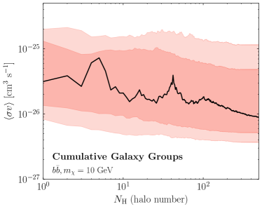
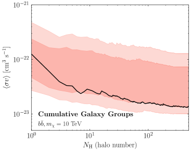
Other Annihilation Channels. In general, DM may annihilate to a variety of Standard Model final states. Figure B.2 (right) interprets the results of the analysis in terms of limits on additional final states that also lead to continuum gamma-ray emission. Final states that predominantly decay hadronically (, , , , , ) give similar limits because their energy spectra are mostly set by boosted pion decay. The leptonic channels (, ) give weaker limits because gamma-rays predominantly arise from final-state radiation or, in the case of the muon, radiative decays. The limit is intermediate because roughly 35% of the decays are leptonic, while the remaining are hadronic. Of course, the DM could annihilate into even more complicated final states than the two-body cases considered here and the results can be extended to these cases [305, 306]. Note that the limits we present for the leptonic final states are conservative, as they neglect Inverse Compton (IC) emission and electromagnetic cascades, which are likely important at high DM masses—see e.g., Ref. [338, 339]. A more careful treatment of these final states requires modeling the magnetic field strength and energy loss mechanisms within the galaxy groups.
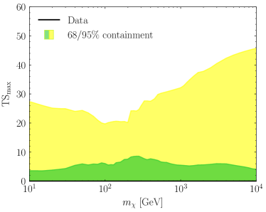
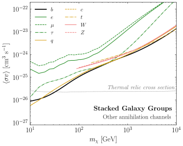
Injected Signal. An important consistency requirement is to ensure that the limit-setting procedure does not exclude a putative DM signal. The likelihood procedure employed here was extensively vetted in Ch. 4, where we demonstrated that the limit never excludes an injected signal. In Fig. B.3, we demonstrate a data-driven version of this test. In detail, we inject a DM signal on top of the actual data set used in the main analysis, focusing on the case of DM annihilation to for a variety of cross sections and masses. We then apply the analysis pipeline to these maps. The top panel of Fig. B.3 shows the recovered cross sections, as a function of the injected values. The green line corresponds to the 95% cross section limit, while the blue line shows the best-fit cross section. Note that statistical uncertainties arising from DM annihilation photon counts are not significant here, as the dominant source of counts arises from the data itself. The columns correspond to 10, 100, and 104 GeV DM annihilating to (left, center, right, respectively). The bottom row shows the maximum test statistic in favor of the model with DM as a function of the injected cross section. The best-fit cross sections are only meaningful when the maximum test statistic is , implying evidence for DM annihilation. We see that across all masses, the cross section limit (green line) is always weaker than the injected value. Additionally, the recovered cross section (blue line) closely approaches that of the injected signal as the significance of the DM excess increases.
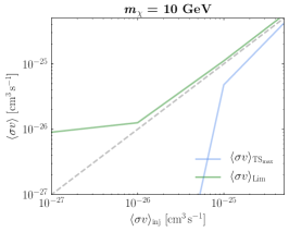
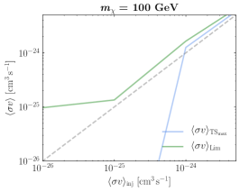
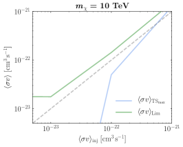
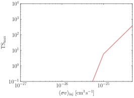
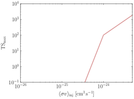
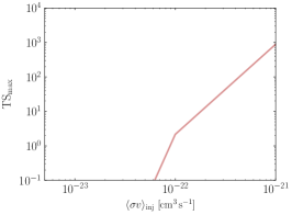
Results for Individual Halos. Here, we explore the properties of the individual galaxy groups that are included in the stacked analysis. These galaxy groups are taken from the catalogs in Ref. [132] and [133], which we refer to as T15 and T17, respectively. Table B.1 lists the top 25 galaxy groups, ordered by the relative brightness of their inferred -factor. If a group in the table is not labeled with a checkmark, then it is not included in the stacking because one of the following conditions is met:
| (B.2) |
Note that the overlap criteria is applied sequentially in order of increasing -factor. These selection criteria have been extensively studied on mock data in Ch. 4 and have been verified to not exclude a potential DM signal, even on data as discussed above. Of the five halos with the largest -factors that are excluded, Andromeda is removed because of its large angular extent, and the rest fail the latitude cut.
The exclusion of Andromeda is not a result of the criteria in Eq. B.2, so some more justification is warranted. As can be seen in Table B.1, the angular extent of Andromeda’s scale radius, , is significantly larger than that of any other halo. To justify as a proxy for angular extent of the emission, we calculate the 68% (95%) containment angle of the expected DM annihilation flux, without accounting for the PSF, and find 1.2∘ (4.4∘). This can be contrasted with the equivalent numbers for the next most important halo, Virgo, where the corresponding 68% (95%) containment angles are 0.5∘ (2.0∘). Because Andromeda is noticeably more extended beyond the Fermi PSF, one must carefully model the spatial distribution of both the smooth DM component and the substructure. Such a dedicated analysis of Andromeda was recently performed by the Fermi collaboration [286]. Out of an abundance of caution, we remove Andromeda from the main joint analysis, but we do show how the limits change when Andromeda is included further below.
Figure LABEL:fig:individual_lims shows the individual limits on the annihilation cross section for the top ten halos that pass the selection cuts and Fig. LABEL:fig:individual_maxts shows the maximum test statistic (TS), as a function of , for these same halos. The green and yellow bands in Fig. LABEL:fig:individual_lims and LABEL:fig:individual_maxts represent the 68% and 95% containment regions obtained by randomly changing the sky location of each individual halo 200 times (subject to the selection criteria listed above). As is evident, the individual limits for the halos are consistent with expectation under the null hypothesis—i.e., the black line falls within the green/yellow bands for each of these halos. Some of these groups have been analyzed in previous cluster studies. For example, the Fermi Collaboration provided DM bounds for Virgo [116]; our limit is roughly consistent with theirs, and possibly a bit stronger, though an exact comparison is difficult to make due to differences in the data set and DM model assumptions.***Note that the -factor in Ref. [116] is a factor of too small.
Figure LABEL:fig:individual_flux provides the 95% upper limits on the gamma-ray flux associated with the DM template for each of the top ten halos. The upper limits are provided for 26 energy bins and compared to the expectations under the null hypothesis. The upper limits are generally consistent with the expectations under the null hypothesis, though small systematic discrepancies do exist for a few halos, such as NGC3031, at high energies. This could be due to subtle differences in the sky locations and angular extents between the objects of interest and the set of representative halos used to create the null hypothesis expectations.
To demonstrate the case of a galaxy group with an excess, we show the TS distribution and the limit for NGC6822 in Fig. B.4. This object fails the selection criteria because it is too close to the Galactic plane. However, it also exhibits a TS excess and, as expected, the limit is weaker than the expectation under the null hypothesis.
Sky maps. In Fig. LABEL:fig:individual_skyrois, we show the counts map in square regions around each of the top nine halos that pass the selection cuts. For each map, we show all photons with energies above 500 MeV, indicate all Fermi 3FGL point sources with orange stars, and show the extent of with a dashed orange circle. Given a DM signal, we would expect to see emission extend out to at the center of these images.
| Name | TS | Incl. | ||||||||
| [GeV2 cm-5 sr] | [] | [deg] | [deg] | [deg] | ||||||
| Andromeda | 19.790.36 | 12.40.12 | 0.17 | 121.51 | -21.79 | 1.040.17 | 2.57 | 2.64 | 2.92 | |
| NGC4472/Virgo | 19.110.35 | 14.60.14 | 3.58 | 283.94 | 74.52 | 0.800.18 | 1.15 | 4.53 | 1.04 | ✓ |
| NGC5128 | 18.890.37 | 12.90.12 | 0.82 | 307.88 | 17.08 | 0.990.17 | 0.88 | 3.14 | 0.00 | |
| NGC0253 | 18.760.37 | 12.70.12 | 0.79 | 98.24 | -87.89 | 1.000.17 | 0.77 | 2.90 | 0.63 | ✓ |
| Maffei 1 | 18.680.37 | 12.60.12 | 0.78 | 136.23 | -0.44 | 1.010.17 | 0.71 | 2.81 | 7.26 | |
| NGC6822 | 18.590.37 | 10.70.10 | 0.11 | 25.34 | -18.40 | 1.170.17 | 0.77 | 1.70 | 16.65 | |
| NGC3031 | 18.580.36 | 12.60.12 | 0.83 | 141.88 | 40.87 | 1.020.17 | 0.64 | 2.76 | 0.00 | ✓ |
| NGC4696/Centaurus | 18.330.35 | 14.60.14 | 8.44 | 302.22 | 21.65 | 0.800.18 | 0.47 | 4.50 | 6.60 | ✓ |
| NGC1399 | 18.300.37 | 13.80.13 | 4.11 | 236.62 | -53.88 | 0.890.17 | 0.45 | 3.87 | 0.72 | ✓ |
| IC0356 | 18.260.36 | 13.50.13 | 3.14 | 138.06 | 12.70 | 0.920.17 | 0.43 | 3.51 | 0.02 | |
| NGC4594 | 18.260.35 | 13.30.13 | 2.56 | 299.01 | 51.30 | 0.940.17 | 0.43 | 3.36 | 0.00 | ✓ |
| IC1613 | 18.170.37 | 10.60.10 | 0.17 | 129.74 | -60.58 | 1.180.17 | 0.48 | 1.67 | 1.72 | |
| Norma | 18.160.33 | 15.10.15 | 17.07 | 325.29 | -7.21 | 0.740.18 | 0.39 | 5.17 | 0.00 | ✓ |
| NGC4736 | 18.120.36 | 12.20.12 | 1.00 | 124.83 | 75.76 | 1.050.17 | 0.38 | 2.58 | 0.00 | |
| NGC1275/Perseus | 18.120.33 | 15.00.15 | 17.62 | 150.58 | -13.26 | 0.750.18 | 0.37 | 5.16 | 0.93 | ✓ |
| NGC3627 | 18.110.35 | 13.00.13 | 2.20 | 241.46 | 64.36 | 0.980.17 | 0.35 | 3.23 | 27.24 | |
| NGC1316/Fornax | 18.010.36 | 13.50.13 | 4.17 | 239.98 | -56.68 | 0.920.17 | 0.32 | 3.49 | 2.33 | |
| NGC5236 | 18.010.36 | 12.20.12 | 1.09 | 314.58 | 31.98 | 1.050.17 | 0.33 | 2.56 | 22.08 | |
| IC0342 | 18.000.37 | 11.80.11 | 0.73 | 138.52 | 10.69 | 1.090.17 | 0.34 | 2.33 | 1.92 | |
| NGC4565 | 17.970.35 | 13.10.13 | 2.98 | 229.92 | 86.07 | 0.960.17 | 0.30 | 3.28 | 41.15 | |
| Coma | 17.960.33 | 15.20.15 | 24.45 | 57.20 | 87.89 | 0.730.18 | 0.31 | 5.21 | 2.35 | ✓ |
| NGC1553/Dorado | 17.940.36 | 13.40.13 | 4.02 | 265.56 | -43.51 | 0.940.17 | 0.30 | 3.41 | 0.08 | ✓ |
| NGC3311/Hydra | 17.940.34 | 14.40.14 | 10.87 | 269.55 | 26.41 | 0.820.17 | 0.30 | 4.32 | 0.04 | ✓ |
| NGC3379 | 17.930.37 | 12.90.12 | 2.42 | 233.64 | 57.77 | 0.990.17 | 0.29 | 3.11 | 0.00 | ✓ |
| NGC5194 | 17.930.37 | 12.60.12 | 1.84 | 104.86 | 68.53 | 1.010.17 | 0.30 | 2.81 | 4.94 | ✓ |
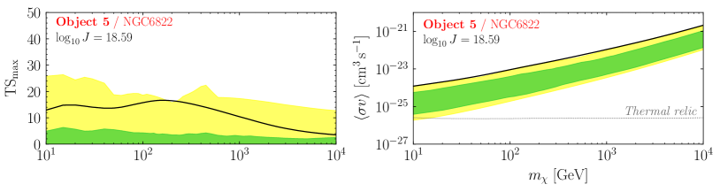
B.2 Variations on the Analysis
We have performed a variety of systematic tests to understand the robustness of the results presented in the main body of the analysis. Several of these uncertainties are discussed in detail in Ch. 4; here, we focus specifically on how they affect the results of the data analysis.
Halo Selection Criteria. Here, we demonstrate how variations on the halo selection conditions listed above affect the baseline results of Fig. 5.1. In the left panel of Fig. B.5, the red line shows the limit that is obtained when starting with 10,000 halos instead of 1000, but requiring the same selection conditions. Despite the modest improvement in the limit, we choose to use 1000 halos in the baseline study because systematically testing the robustness of the analysis procedure, as done in Ch. 4, becomes computationally prohibitive otherwise. In order to calibrate the analysis for higher halo numbers, it would be useful to use semi-analytic methods to project the sensitivity, such as those discussed in Ref. [340, 341], although we leave the details to future work.
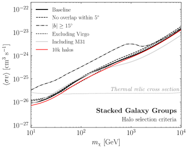
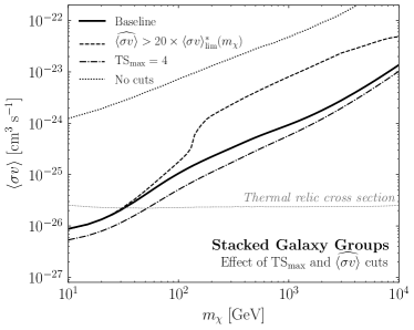
Virgo is the object with the highest -factor in the stacked sample. As made clear in the dedicated study of this object by the Fermi Collaboration [116], there are challenges associated with modeling the diffuse emission in Virgo’s vicinity. However, we emphasize that the baseline limit is not highly sensitive to any one halo, including the brightest in the sample. For example, the dotted line in the left panel of Fig. B.5 shows the impact on the limit after removing Virgo from the stacking. Critically, we see that the limit is almost unchanged, highlighting that the stacked result is not solely driven by the object with the largest -factor.
The effect of including Andromeda (M31) is shown as the gray solid line. We exclude Andromeda from the baseline analysis because of its large angular size, as discussed in detail above. Our analysis relies on the assumption that the DM halos are approximately point-like on the sky, which fails for Andromeda, and we therefore deem it to fall outside the scope of the systematic studies performed here.
The dashed line shows the effect of tightening the condition on overlapping halos from to . Predictably, the limit is slightly weakened due to the smaller pool of available targets. We also show the effect of decreasing the latitude cut to (dot-dashed line). In this case, the number of halos included in the stacked analysis increases, but the limit is weaker—considerably so below GeV. The weakened limits are likely due to enhanced diffuse emission along the plane as well as contributions from unresolved point sources, both of which are difficult to accurately model. In cases with such mismodeling, the addition of a DM template can generically improve the quality of the fit, which leads to excesses at low energies, in particular. The baseline latitude cut ameliorates precisely these concerns.
The right panel of Fig. B.5 illustrates the effects of changing, or removing completely, the cross section and TS cuts on the halos. Specifically, the dashed black line shows what happens when we require that a halo’s excess be even more inconsistent with the limits set by other galaxy groups; specifically, requiring that . The dot-dashed line shows the limit when we decrease the statistical significance requirement to . Note that the two changes have opposite effects on the limits. This is expected because more halos with excesses are included in the stacking procedure with the more stringent cross section requirement, which weakens the limit, whereas fewer are included if we reduce the TS cut, strengthening the limit.
The dotted line in the right panel of Fig. B.5 shows what happens when no requirement at all is placed on the TS and cross section; in this case, the limit is dramatically weakened by several orders of magnitude. We show the same result in Fig. B.6 (dotted line), but with a comparison to the null hypothesis corresponding to no TS and cross section cuts, which is shown as the 68% (95%) red (blue) bands.†††We thank A. Drlica-Wagner for suggesting this test. In the baseline case, the limit is consistent with the random sky locations—i.e., the solid black line falls within the green/yellow bands. However, with no TS and cross section cuts, this is no longer true—i.e., the dotted black line falls outside the red/blue bands. Clear excesses are observed above the background expectation in this case, but they are inconsistent with a DM interpretation as they are strongly excluded by other halos in the stack. When deciding on the TS and cross section requirements that we used for the baseline analysis in Fig. 5.1, our goal was to maximize the sensitivity reach while simultaneously ensuring that an actual DM signal would not be excluded. We verified the selection criteria thoroughly by performing injected signal tests on the data (discussed above) as well as on mock data (discussed in Ch. 4). Ideally, galaxy groups would be excluded from the stacking based on the specific properties of the astrophysical excesses that they exhibit, as opposed to the TS and cross section requirements used here. For example, one can imagine excluding groups that are known to host AGN or galaxies with high amounts of star-formation activity. We plan to study such possibilities in future work.
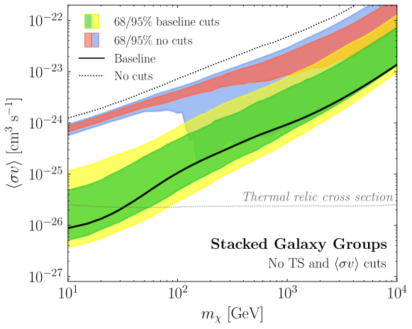
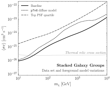
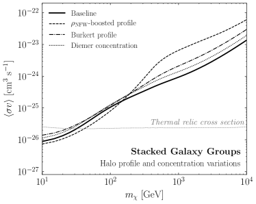
Data Set and Foreground Models. In the results presented thus far, we have used all quartiles of the UltracleanVeto event class of the Fermi data. Alternatively, we can restrict ourselves to the top quartile of events, as ranked by PSF. Using this subset of data has the advantage of improved angular resolution, but the disadvantage of a 75% reduction in statistics. The left panel of Fig. B.7 shows the limit (dot-dashed line) obtained by repeating the analysis with the top quartile of UltracleanVeto data; the bounds are weaker than in the all-quartile case, as would be expected. However, the amount by which the limit weakens is not completely consistent with the decrease in statistics. Rather, it appears that when we lower the photon statistics, more halos that were previously excluded by the cross section and TS criteria in the baseline analysis are allowed into the stacking and collectively weaken the limit.
Another choice that we made for the baseline analysis was to use the p8r2 foreground model for gamma-ray emission from cosmic-ray processes in the Milky Way. In this model, the bremsstrahlung and boosted pion emission are traced with gas column-density maps and the IC emission is modeled using Galprop [271]. After fitting the data with these three components, any ‘extended emission excesses’ are identified and added back into the foreground model [342]. To study the dependence of the results on the choice of foreground model, we repeat the analysis using the Pass 7 gal_2yearp7v6_v0.fits (p7v6) model, which includes large-scale structures like Loop 1 and the Fermi bubbles—in addition to the bremsstrahlung, pion, and IC emission—but does not account for any data-driven excesses as is done in p8r2. The results of the stacked analysis using the p7v6 model are shown in the left panel of Fig. B.7 (dashed line). The limit is somewhat weaker to that obtained using p8r2, though it is broadly similar to the latter. This is to be expected for stacked analyses, where the dependence on mismodeling of the foreground emission is reduced because the fits are done on small, independent regions of the sky, so that offsets in the point-to-point normalizations of the diffuse model can have less impact. For more discussion of this point, see Ref. [95, 161, 343, 344].
Halo Density Profile and Concentration. Our baseline analysis makes two assumptions about the profiles of gamma-ray emission from the extragalactic halos. The first assumption is that the DM profile of the smooth halo is described by an NFW profile:
| (B.3) |
where is the normalization and the scale radius [326]. The NFW profile successfully describes the shape of cluster-size DM halos in -body simulations with and without baryons (see, e.g., Ref. [138, 345]). However, some evidence exists pointing to cored density profiles on smaller scales (e.g., dwarf galaxies), and the density profiles in these systems may be better described by the phenomenological Burkert profile [337]:
| (B.4) |
where and are the Burkert corollaries to the NFW and , but have numerically different values. While it appears unlikely that the Burkert profile is a good description of the DM profiles of the cluster-scale halos considered here, using this profile provides a useful systematic variation because it predicts less annihilation flux than the NFW profile does. The right panel of Fig. B.7 shows the effect of using the Burkert profile to describe the halos in the T15 and T17 catalogs (dot-dashed line); the limit is slightly weaker, as expected.
The second assumption we made is that the shape of the gamma-ray emission from DM annihilation follows the projected integral of the DM-distribution squared. This is likely incorrect because the contribution from the boost factor, which can be substantial, should have the spatial morphology of the distribution of DM subhalos. Neglecting tidal effects, we expect the subhalos to follow the DM distribution (instead of the squared distribution). Including tidal effects is complicated, as subhalos closer to the halo center are more likely to be tidally stripped, which both increases their concentration and decreases their number density. We do not attempt to model the change in the spatial morphology of the subhalo distribution from tidal stripping and instead consider the limit where the annihilation flux from the subhalo boost follows the NFW distribution. This gives a much wider angular profile for the annihilation flux for large clusters, compared to the case where the boost is simply a multiplicative factor. The dashed line in the right panel of Fig. B.7 shows the effect on the limit of modeling the gamma-ray emission in this way (labeled “-boosted profile”). The extended spatial profile leads to a minimal change in the limit over most of the mass range, which is to be expected given that most of the galaxy groups can be well-approximated as point sources.
A halo’s virial concentration is an indicator of its overall density and is defined as , where is the virial radius and the NFW scale radius of the halo. A variety of models exist in the literature that map from halo mass to concentration. Our fiducial case is the Correa et al. model from Ref. [311]. Here we show how the limit (dotted line) changes when we use the model of Diemer and Kravtsov [312], updated with the Planck 2015 cosmology [20]. The change to the limit is minimal, which is perhaps a reflection of the fact that the change in the mean concentrations between the concentration-mass models is small compared to the statistical spread predicted in these models, which is incorporated into the -factor uncertainties. We have also verified that increasing the dispersion on the concentration for the Correa et al. model to 0.24 [346], which is above the 0.14–0.19 range used in the baseline study, worsens the limit by a factor.
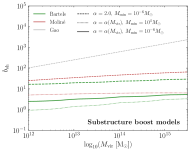
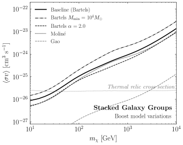
Substructure Boost. Hierarchical structure formation implies that larger structures can host smaller substructures, the presence of which can significantly enhance signatures of DM annihilation in host halos. Although several models exist in the literature to characterize this effect, the precise enhancement sensitively depends on the methods used as well as the astrophysical and particle physics properties that are assumed. Phenomenological extrapolation of subhalo properties (e.g., the concentration-mass relation) over many orders of magnitude down to very small masses ) M⊙ lead to large enhancements of and for galaxy- and cluster-sized halos, respectively [315]. Recent numerical simulations and analytic studies [327, 311, 328] suggest that the concentration-mass relation flattens at smaller masses, yielding boosts that are much more modest, about an order-of-magnitude below phenomenological extrapolations [347, 139]. In addition, the concentration-mass relation for field halos cannot simply be applied to subhalos, because the latter undergo tidal stripping as they fall into and orbit their host. Such effects tend to make the subhalos more concentrated—and therefore more luminous—than their field-halo counterparts, though the number-density of such subhalos is also reduced [307].
When taken together, the details of the halo formation process shape the subhalo mass function , where . The mass function does not follow a power-law to arbitrarily low masses, however, because the underlying particle physics model for the DM can place a minimum cutoff on the subhalo mass, . For example, DM models with longer free-streaming lengths wash out smaller-scale structures, resulting in higher cutoffs.
The left panel of Fig. B.8 shows a variety of boost models commonly used in DM studies. The fiducial boost model used here [307] is shown as the thick green solid line and variations on and are also plotted. The right panel of Fig. B.8 shows that the expected limit when M⊙ instead of M⊙ (dot-dashed) is weaker across all masses. While a minimum subhalo mass of M⊙ is likely inconsistent with bounds on the kinetic decoupling temperature of thermal DM, this example illustrates the importance played by in the sensitivity reach. Additionally, Fig. B.8 demonstrates the case where (dashed line). Increasing the inner slope of the subhalo mass function leads to a correspondingly stronger limit, however observations tend to favor a slope closer to (which is what the most massive halos correspond to in our fiducial case).
Ref. [139] derived a boost factor model that accounts for the flattening of the concentration-mass relation at low masses, but does not include the effect of tidal stripping. They assume a minimum sub-halo mass of M⊙ and a halo-mass function . This was updated by Ref. [314] to account for the effect of tidal disruption. This updated boost factor model, which takes , gives the constraint shown in Fig. B.8 labeled “Moliné” (dotted). This model is to be contrasted with the boost factor model of Ref. [315], labeled “Gao” in Fig. B.8 (grey-dashed), which uses a phenomenological power-law extrapolation of the concentration-mass relation to low sub-halo masses. Because the annihilation rate increases with increasing concentration parameter, the model in Ref. [315] predicts substantially larger boosts than other scenarios that take into account a more realistic flattening of the concentration-mass relation at low subhalo masses.
Galaxy Group Catalog.
We now explore the dependence of the results on the group catalog that is used to select the halos. In this way, we can better understand how the DM bounds are affected by uncertainties on galaxy clustering algorithms and the inference of the virial mass of the halos. The baseline limits are based on the T15 and T17 catalogs, but here we repeat the analysis using the Lu et al. catalog [295], which solely relies on 2MRS observations. The group-finding algorithm used by Ref. [295] is different to that of T15 and T17 in many ways, relying on a friends-of-friends algorithm as opposed to one based on matching group properties at different scales to -body simulations. Lu et al. also use a different halo mass determination. For these reasons, it provides a good counterpoint to T15 and T17 for estimating systematic uncertainties associated with the identification of galaxy groups. While T17 includes measured distances for nearby groups, the Lu catalog corrects for the effect of peculiar velocities following the prescription in Ref. [348] and the effect of Virgo infall as in Ref. [349]. Figure B.9 is a repeat of Fig. 5.1 in the main analysis, except using the Lu et al. catalog. Despite important differences between the group catalogs used, the Lu et al. results are very similar to the baseline case.
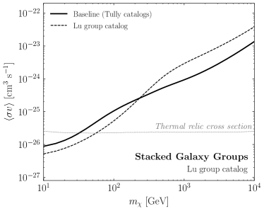
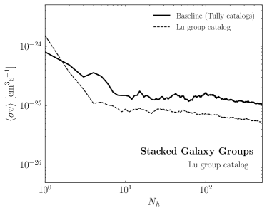
There are a variety of sources of systematic uncertainty beyond those described here that deserve further study. For example, a systematic bias in the -factor determination due to offsets in either the mass inference or the concentration-mass relation can be a potential source of uncertainty. A better understanding of the galaxy-halo connection and the small-scale structure of halos is required to mitigate this. Furthermore, we assumed distance uncertainties to be subdominant in our analysis. While this is certainly a good assumption over the redshift range of interest—nearby groups have measured distances, while groups further away come with spectroscopic redshift measurements with small expected peculiar velocity contamination—uncertainties on these do exist. We have also assumed that our targets consist of virialized halos and have not accounted for possible out-of-equilibrium effects in modeling these [350].
References
- [1] M. Lisanti, “Lectures on Dark Matter Physics,” in Proceedings, Theoretical Advanced Study Institute in Elementary Particle Physics: New Frontiers in Fields and Strings (TASI 2015): Boulder, CO, USA, June 1-26, 2015, pp. 399–446. 2017. arXiv:1603.03797 [hep-ph]. http://inspirehep.net/record/1427360/files/arXiv:1603.03797.pdf.
- [2] T. Plehn, “Yet Another Introduction to Dark Matter,” arXiv:1705.01987 [hep-ph].
- [3] T. R. Slatyer, “Indirect Detection of Dark Matter,” in Proceedings, Theoretical Advanced Study Institute in Elementary Particle Physics : Anticipating the Next Discoveries in Particle Physics (TASI 2016): Boulder, CO, USA, June 6-July 1, 2016, pp. 297–353. 2018. arXiv:1710.05137 [hep-ph].
- [4] G. Bertone and D. Hooper, “A History of Dark Matter,” Submitted to: Rev. Mod. Phys. (2016) , arXiv:1605.04909 [astro-ph.CO].
- [5] J. C. Kapteyn, “First Attempt at a Theory of the Arrangement and Motion of the Sidereal System,”ApJ 55 (May, 1922) 302.
- [6] J. H. Oort, “The force exerted by the stellar system in the direction perpendicular to the galactic plane and some related problems,”Bull. Astron. Inst. Netherlands 6 (Aug., 1932) 249.
- [7] J. H. Jeans, “The Motions of Stars in a Kapteyn Universe,”MNRAS 82 (Jan., 1922) 122–132.
- [8] E. Hubble and M. L. Humason, “The Velocity-Distance Relation among Extra-Galactic Nebulae,”ApJ 74 (July, 1931) 43.
- [9] F. Zwicky, “Die Rotverschiebung von extragalaktischen Nebeln,” Helvetica Physica Acta 6 (1933) 110–127.
- [10] F. Zwicky, “On the Masses of Nebulae and of Clusters of Nebulae,”ApJ 86 (Oct., 1937) 217.
- [11] H. W. Babcock, “The rotation of the Andromeda Nebula,” Lick Observatory Bulletin 19 (1939) 41–51.
- [12] V. C. Rubin and W. K. Ford, Jr., “Rotation of the Andromeda Nebula from a Spectroscopic Survey of Emission Regions,”ApJ 159 (Feb., 1970) 379.
- [13] M. S. Roberts and A. H. Rots, “Comparison of Rotation Curves of Different Galaxy Types,”A&A 26 (Aug., 1973) 483–485.
- [14] J. Einasto, A. Kaasik, and E. Saar, “Dynamic evidence on massive coronas of galaxies,”Nature 250 (July, 1974) 309–310.
- [15] J. P. Ostriker, P. J. E. Peebles, and A. Yahil, “The size and mass of galaxies, and the mass of the universe,”ApJ 193 (Oct., 1974) L1–L4.
- [16] Y. Sofue, M. Honma, and T. Omodaka, “Unified Rotation Curve of the Galaxy – Decomposition into de Vaucouleurs Bulge, Disk, Dark Halo, and the 9-kpc Rotation Dip –,”PASJ 61 (Feb., 2009) 227–236, arXiv:0811.0859.
- [17] S. Dodelson, Modern cosmology. Academic Press, San Diego, CA, 2003. https://cds.cern.ch/record/1282338.
- [18] E. W. Kolb and M. S. Turner, “The Early Universe,” Front. Phys. 69 (1990) 1–547.
- [19] G. Hinshaw, D. Larson, E. Komatsu, D. N. Spergel, C. L. Bennett, J. Dunkley, M. R. Nolta, M. Halpern, R. S. Hill, N. Odegard, L. Page, K. M. Smith, J. L. Weiland, B. Gold, N. Jarosik, A. Kogut, M. Limon, S. S. Meyer, G. S. Tucker, E. Wollack, and E. L. Wright, “Nine-year Wilkinson Microwave Anisotropy Probe (WMAP) Observations: Cosmological Parameter Results,”ApJS 208 (Oct., 2013) 19, arXiv:1212.5226.
- [20] Planck Collaboration, P. A. R. Ade et al., “Planck 2015 results. XIII. Cosmological parameters,” Astron. Astrophys. 594 (2016) A13, arXiv:1502.01589 [astro-ph.CO].
- [21] A. Lewis, A. Challinor, and A. Lasenby, “Efficient computation of CMB anisotropies in closed FRW models,” Astrophys. J. 538 (2000) 473–476, arXiv:astro-ph/9911177 [astro-ph].
- [22] BOSS Collaboration, S. Alam et al., “The clustering of galaxies in the completed SDSS-III Baryon Oscillation Spectroscopic Survey: cosmological analysis of the DR12 galaxy sample,” Mon. Not. Roy. Astron. Soc. 470 (2017) no. 3, 2617–2652, arXiv:1607.03155 [astro-ph.CO].
- [23] DES Collaboration, T. M. C. Abbott et al., “Dark Energy Survey Year 1 Results: Cosmological Constraints from Galaxy Clustering and Weak Lensing,” arXiv:1708.01530 [astro-ph.CO].
- [24] S. Vegetti, L. V. E. Koopmans, A. Bolton, T. Treu, and R. Gavazzi, “Detection of a dark substructure through gravitational imaging,”MNRAS 408 (Nov., 2010) 1969–1981, arXiv:0910.0760.
- [25] S. Vegetti, D. J. Lagattuta, J. P. McKean, M. W. Auger, C. D. Fassnacht, and L. V. E. Koopmans, “Gravitational detection of a low-mass dark satellite galaxy at cosmological distance,”Nature 481 (Jan., 2012) 341–343, arXiv:1201.3643.
- [26] D. Clowe et al., “A direct empirical proof of the existence of dark matter,” Astrophys. J. 648 (2006) L109–L113, astro-ph/0608407.
- [27] M. Milgrom, “A modification of the Newtonian dynamics as a possible alternative to the hidden mass hypothesis,”ApJ 270 (July, 1983) 365–370.
- [28] M. Milgrom, “A modification of the Newtonian dynamics - Implications for galaxies,”ApJ 270 (July, 1983) 371–389.
- [29] M. Milgrom, “A Modification of the Newtonian Dynamics - Implications for Galaxy Systems,”ApJ 270 (July, 1983) 384.
- [30] R. B. Tully and J. R. Fisher, “A new method of determining distances to galaxies,”A&A 54 (Feb., 1977) 661–673.
- [31] J. D. Bekenstein, “Relativistic gravitation theory for the MOND paradigm,” Phys. Rev. D70 (2004) 083509, arXiv:astro-ph/0403694 [astro-ph]. [Erratum: Phys. Rev.D71,069901(2005)].
- [32] C. Skordis, “TOPICAL REVIEW: The tensor-vector-scalar theory and its cosmology,”Classical and Quantum Gravity 26 (July, 2009) 143001, arXiv:0903.3602 [astro-ph.CO].
- [33] B. Famaey and S. McGaugh, “Modified Newtonian Dynamics (MOND): Observational Phenomenology and Relativistic Extensions,” Living Rev. Rel. 15 (2012) 10, arXiv:1112.3960 [astro-ph.CO].
- [34] S. S. Gershtein and Ya. B. Zeldovich, “Rest Mass of Muonic Neutrino and Cosmology,” JETP Lett. 4 (1966) 120–122. [,58(1966)].
- [35] R. Cowsik and J. McClelland, “An upper limit on the neutrino rest mass,”Phys. Rev. Lett. 29 (Sep, 1972) 669–670. https://link.aps.org/doi/10.1103/PhysRevLett.29.669.
- [36] B. W. Lee and S. Weinberg, “Cosmological lower bound on heavy-neutrino masses,”Phys. Rev. Lett. 39 (Jul, 1977) 165–168. https://link.aps.org/doi/10.1103/PhysRevLett.39.165.
- [37] J. E. Gunn, B. W. Lee, I. Lerche, D. N. Schramm, and G. Steigman, “Some astrophysical consequences of the existence of a heavy stable neutral lepton,”ApJ 223 (Aug., 1978) 1015–1031.
- [38] S. D. M. White, C. S. Frenk, and M. Davis, “Clustering in a neutrino-dominated universe,”ApJ 274 (Nov., 1983) L1–L5.
- [39] J. Wess and B. Zumino, “Supergauge Transformations in Four-Dimensions,” Nucl. Phys. B70 (1974) 39–50. [,24(1974)].
- [40] H. Pagels and J. R. Primack, “Supersymmetry, cosmology, and new physics at teraelectronvolt energies,”Phys. Rev. Lett. 48 (Jan, 1982) 223–226. https://link.aps.org/doi/10.1103/PhysRevLett.48.223.
- [41] G. Jungman, M. Kamionkowski, and K. Griest, “Supersymmetric dark matter,” Phys. Rept. 267 (1996) 195–373, arXiv:hep-ph/9506380.
- [42] S. Dimopoulos and H. Georgi, “Softly Broken Supersymmetry and SU(5),” Nucl. Phys. B193 (1981) 150–162.
- [43] G. Bertone, D. Hooper, and J. Silk, “Particle dark matter: Evidence, candidates and constraints,” Phys. Rept. 405 (2005) 279–390, hep-ph/0404175.
- [44] S. Weinberg, “A new light boson?,”Phys. Rev. Lett. 40 (Jan, 1978) 223–226. https://link.aps.org/doi/10.1103/PhysRevLett.40.223.
- [45] R. D. Peccei and H. R. Quinn, “CP Conservation in the Presence of Instantons,” Phys. Rev. Lett. 38 (1977) 1440–1443. [,328(1977)].
- [46] K. Abazajian, G. M. Fuller, and M. Patel, “Sterile neutrino hot, warm, and cold dark matter,” Phys. Rev. D64 (2001) 023501, arXiv:astro-ph/0101524 [astro-ph].
- [47] U. Seljak, A. Makarov, P. McDonald, and H. Trac, “Can sterile neutrinos be the dark matter?,” Phys. Rev. Lett. 97 (2006) 191303, arXiv:astro-ph/0602430 [astro-ph].
- [48] J. L. Feng and J. Kumar, “The WIMPless Miracle: Dark-Matter Particles without Weak- Scale Masses or Weak Interactions,” Phys. Rev. Lett. 101 (2008) 231301, arXiv:0803.4196 [hep-ph].
- [49] T. Lin, H.-B. Yu, and K. M. Zurek, “On Symmetric and Asymmetric Light Dark Matter,” Phys. Rev. D85 (2012) 063503, arXiv:1111.0293 [hep-ph].
- [50] L. Hui, J. P. Ostriker, S. Tremaine, and E. Witten, “Ultralight scalars as cosmological dark matter,” Phys. Rev. D95 (2017) no. 4, 043541, arXiv:1610.08297 [astro-ph.CO].
- [51] J. Zhang, J.-L. Kuo, H. Liu, Y.-L. S. Tsai, K. Cheung, and M.-C. Chu, “Is Fuzzy Dark Matter in tension with Lyman-alpha forest?,” arXiv:1708.04389 [astro-ph.CO].
- [52] S. Horiuchi, P. J. Humphrey, J. Onorbe, K. N. Abazajian, M. Kaplinghat, and S. Garrison-Kimmel, “Sterile neutrino dark matter bounds from galaxies of the Local Group,” Phys. Rev. D89 (2014) no. 2, 025017, arXiv:1311.0282 [astro-ph.CO].
- [53] K. Griest, A. M. Cieplak, and M. J. Lehner, “Experimental Limits on Primordial Black Hole Dark Matter from the First 2 yr of Kepler Data,” Astrophys. J. 786 (2014) no. 2, 158, arXiv:1307.5798 [astro-ph.CO].
- [54] T. Bringmann and S. Hofmann, “Thermal decoupling of WIMPs from first principles,” JCAP 0704 (2007) 016, arXiv:hep-ph/0612238 [hep-ph]. [Erratum: JCAP1603,no.03,E02(2016)].
- [55] M. Viel, G. D. Becker, J. S. Bolton, and M. G. Haehnelt, “Warm dark matter as a solution to the small scale crisis: New constraints from high redshift Lyman- forest data,” Phys. Rev. D88 (2013) 043502, arXiv:1306.2314 [astro-ph.CO].
- [56] K. Griest and M. Kamionkowski, “Unitarity Limits on the Mass and Radius of Dark Matter Particles,” Phys. Rev. Lett. 64 (1990) 615.
- [57] P. Gondolo and G. Gelmini, “Cosmic abundances of stable particles: improved analysis.,”Nuclear Physics B 360 (Aug., 1991) 145–179.
- [58] XENON Collaboration, E. Aprile et al., “Dark Matter Search Results from a One TonneYear Exposure of XENON1T,” arXiv:1805.12562 [astro-ph.CO].
- [59] DarkSide Collaboration, P. Agnes et al., “Low-Mass Dark Matter Search with the DarkSide-50 Experiment,” arXiv:1802.06994 [astro-ph.HE].
- [60] M. Escudero, A. Berlin, D. Hooper, and M.-X. Lin, “Toward (Finally!) Ruling Out Z and Higgs Mediated Dark Matter Models,” JCAP 1612 (2016) 029, arXiv:1609.09079 [hep-ph].
- [61] Particle Data Group Collaboration, C. Patrignani et al., “Review of Particle Physics,” Chin. Phys. C40 (2016) no. 10, 100001.
- [62] F. Kahlhoefer, “Review of LHC Dark Matter Searches,” Int. J. Mod. Phys. A32 (2017) no. 13, 1730006, arXiv:1702.02430 [hep-ph].
- [63] K. Griest and D. Seckel, “Three exceptions in the calculation of relic abundances,”Phys. Rev. D 43 (May, 1991) 3191–3203. https://link.aps.org/doi/10.1103/PhysRevD.43.3191.
- [64] R. T. D’Agnolo and J. T. Ruderman, “Light Dark Matter from Forbidden Channels,” Phys. Rev. Lett. 115 (2015) no. 6, 061301, arXiv:1505.07107 [hep-ph].
- [65] Y. Hochberg, E. Kuflik, T. Volansky, and J. G. Wacker, “Mechanism for Thermal Relic Dark Matter of Strongly Interacting Massive Particles,” Phys. Rev. Lett. 113 (2014) 171301, arXiv:1402.5143 [hep-ph].
- [66] Y. Hochberg, E. Kuflik, H. Murayama, T. Volansky, and J. G. Wacker, “Model for Thermal Relic Dark Matter of Strongly Interacting Massive Particles,” Phys. Rev. Lett. 115 (2015) no. 2, 021301, arXiv:1411.3727 [hep-ph].
- [67] A. Berlin, D. Hooper, and G. Krnjaic, “Thermal Dark Matter From A Highly Decoupled Sector,” Phys. Rev. D94 (2016) no. 9, 095019, arXiv:1609.02555 [hep-ph].
- [68] A. Berlin, D. Hooper, and G. Krnjaic, “PeV-Scale Dark Matter as a Thermal Relic of a Decoupled Sector,” Phys. Lett. B760 (2016) 106–111, arXiv:1602.08490 [hep-ph].
- [69] A. Berlin and N. Blinov, “Thermal Dark Matter Below an MeV,” Phys. Rev. Lett. 120 (2018) no. 2, 021801, arXiv:1706.07046 [hep-ph].
- [70] N. Bernal, X. Chu, and J. Pradler, “Simply split strongly interacting massive particles,” Phys. Rev. D95 (2017) no. 11, 115023, arXiv:1702.04906 [hep-ph].
- [71] J. M. Cline, H. Liu, T. Slatyer, and W. Xue, “Enabling Forbidden Dark Matter,” Phys. Rev. D96 (2017) no. 8, 083521, arXiv:1702.07716 [hep-ph].
- [72] R. T. D’Agnolo and A. Hook, “Selfish Dark Matter,” Phys. Rev. D91 (2015) no. 11, 115020, arXiv:1504.00361 [hep-ph].
- [73] R. T. D’Agnolo, D. Pappadopulo, and J. T. Ruderman, “Fourth Exception in the Calculation of Relic Abundances,” Phys. Rev. Lett. 119 (2017) no. 6, 061102, arXiv:1705.08450 [hep-ph].
- [74] F. D’Eramo and J. Thaler, “Semi-annihilation of Dark Matter,” JHEP 06 (2010) 109, arXiv:1003.5912 [hep-ph].
- [75] J. A. Dror, E. Kuflik, and W. H. Ng, “Codecaying Dark Matter,” Phys. Rev. Lett. 117 (2016) no. 21, 211801, arXiv:1607.03110 [hep-ph].
- [76] M. Farina, D. Pappadopulo, J. T. Ruderman, and G. Trevisan, “Phases of Cannibal Dark Matter,” JHEP 12 (2016) 039, arXiv:1607.03108 [hep-ph].
- [77] J. Kopp, J. Liu, T. R. Slatyer, X.-P. Wang, and W. Xue, “Impeded Dark Matter,” JHEP 12 (2016) 033, arXiv:1609.02147 [hep-ph].
- [78] E. Kuflik, M. Perelstein, N. R.-L. Lorier, and Y.-D. Tsai, “Elastically Decoupling Dark Matter,” Phys. Rev. Lett. 116 (2016) no. 22, 221302, arXiv:1512.04545 [hep-ph].
- [79] D. Pappadopulo, J. T. Ruderman, and G. Trevisan, “Dark matter freeze-out in a nonrelativistic sector,” Phys. Rev. D94 (2016) no. 3, 035005, arXiv:1602.04219 [hep-ph].
- [80] M. Pospelov, A. Ritz, and M. B. Voloshin, “Secluded WIMP Dark Matter,” Phys. Lett. B662 (2008) 53–61, arXiv:0711.4866 [hep-ph].
- [81] Fermi-LAT Collaboration, W. B. Atwood et al., “The Large Area Telescope on the Fermi Gamma-ray Space Telescope Mission,” Astrophys. J. 697 (2009) 1071–1102, arXiv:0902.1089 [astro-ph.IM].
- [82] HAWC Collaboration, A. U. Abeysekara et al., “Sensitivity of HAWC to high-mass dark matter annihilations,” Phys. Rev. D90 (2014) no. 12, 122002, arXiv:1405.1730 [astro-ph.HE].
- [83] HESS Collaboration, H. Abdallah et al., “Search for -Ray Line Signals from Dark Matter Annihilations in the Inner Galactic Halo from 10 Years of Observations with H.E.S.S.,” Phys. Rev. Lett. 120 (2018) no. 20, 201101, arXiv:1805.05741 [astro-ph.HE].
- [84] MAGIC Collaboration, M. L. Ahnen et al., “Indirect dark matter searches in the dwarf satellite galaxy Ursa Major II with the MAGIC Telescopes,” JCAP 1803 (2018) no. 03, 009, arXiv:1712.03095 [astro-ph.HE].
- [85] VERITAS Collaboration, S. Archambault et al., “Dark Matter Constraints from a Joint Analysis of Dwarf Spheroidal Galaxy Observations with VERITAS,” Phys. Rev. D95 (2017) no. 8, 082001, arXiv:1703.04937 [astro-ph.HE].
- [86] CTA Consortium Collaboration, M. Doro et al., “Dark Matter and Fundamental Physics with the Cherenkov Telescope Array,” Astropart. Phys. 43 (2013) 189–214, arXiv:1208.5356 [astro-ph.IM].
- [87] T. Sjostrand, S. Mrenna, and P. Z. Skands, “A Brief Introduction to PYTHIA 8.1,” Comput.Phys.Commun. 178 (2008) 852–867, arXiv:0710.3820 [hep-ph].
- [88] M. Cirelli, G. Corcella, A. Hektor, G. Hutsi, M. Kadastik, P. Panci, M. Raidal, F. Sala, and A. Strumia, “PPPC 4 DM ID: A Poor Particle Physicist Cookbook for Dark Matter Indirect Detection,” JCAP 1103 (2011) 051, arXiv:1012.4515 [hep-ph]. [Erratum: JCAP1210,E01(2012)].
- [89] DES, Fermi-LAT Collaboration, A. Albert et al., “Searching for Dark Matter Annihilation in Recently Discovered Milky Way Satellites with Fermi-LAT,” Astrophys. J. 834 (2017) no. 2, 110, arXiv:1611.03184 [astro-ph.HE].
- [90] Fermi-LAT Collaboration, M. Ackermann et al., “Searching for Dark Matter Annihilation from Milky Way Dwarf Spheroidal Galaxies with Six Years of Fermi Large Area Telescope Data,” Phys. Rev. Lett. 115 (2015) no. 23, 231301, arXiv:1503.02641 [astro-ph.HE].
- [91] A. Geringer-Sameth, S. M. Koushiappas, and M. G. Walker, “Comprehensive search for dark matter annihilation in dwarf galaxies,” Phys. Rev. D91 (2015) no. 8, 083535, arXiv:1410.2242 [astro-ph.CO].
- [92] J. L. Sanders, N. W. Evans, A. Geringer-Sameth, and W. Dehnen, “Indirect Dark Matter Detection for Flattened Dwarf Galaxies,” Phys. Rev. D94 (2016) no. 6, 063521, arXiv:1604.05493 [astro-ph.GA].
- [93] V. Bonnivard, D. Maurin, and M. G. Walker, “Contamination of stellar-kinematic samples and uncertainty about dark matter annihilation profiles in ultrafaint dwarf galaxies: the example of Segue I,”MNRAS 462 (Oct., 2016) 223–234, arXiv:1506.08209.
- [94] A. Geringer-Sameth, S. M. Koushiappas, and M. Walker, “Dwarf galaxy annihilation and decay emission profiles for dark matter experiments,” Astrophys. J. 801 (2015) no. 2, 74, arXiv:1408.0002 [astro-ph.CO].
- [95] T. Daylan, D. P. Finkbeiner, D. Hooper, T. Linden, S. K. N. Portillo, N. L. Rodd, and T. R. Slatyer, “The characterization of the gamma-ray signal from the central Milky Way: A case for annihilating dark matter,” Phys. Dark Univ. 12 (2016) 1–23, arXiv:1402.6703 [astro-ph.HE].
- [96] L. Goodenough and D. Hooper, “Possible Evidence For Dark Matter Annihilation In The Inner Milky Way From The Fermi Gamma Ray Space Telescope,” arXiv:0910.2998 [hep-ph].
- [97] D. Hooper and L. Goodenough, “Dark Matter Annihilation in The Galactic Center As Seen by the Fermi Gamma Ray Space Telescope,” Phys.Lett. B697 (2011) 412–428, arXiv:1010.2752 [hep-ph].
- [98] F. Calore, I. Cholis, and C. Weniger, “Background model systematics for the Fermi GeV excess,” JCAP 1503 (2015) 038, arXiv:1409.0042 [astro-ph.CO].
- [99] C. Gordon and O. Macias, “Dark Matter and Pulsar Model Constraints from Galactic Center Fermi-LAT Gamma Ray Observations,” Phys.Rev. D88 (2013) 083521, arXiv:1306.5725 [astro-ph.HE].
- [100] Fermi-LAT Collaboration, M. Ajello et al., “Fermi-LAT Observations of High-Energy -Ray Emission Toward the Galactic Center,” Astrophys. J. 819 (2016) no. 1, 44, arXiv:1511.02938 [astro-ph.HE].
- [101] C. Karwin, S. Murgia, T. M. P. Tait, T. A. Porter, and P. Tanedo, “Dark Matter Interpretation of the Fermi-LAT Observation Toward the Galactic Center,” Phys. Rev. D95 (2017) no. 10, 103005, arXiv:1612.05687 [hep-ph].
- [102] S. K. Lee, M. Lisanti, B. R. Safdi, T. R. Slatyer, and W. Xue, “Evidence for Unresolved -Ray Point Sources in the Inner Galaxy,” Phys. Rev. Lett. 116 (2016) no. 5, 051103, arXiv:1506.05124 [astro-ph.HE].
- [103] R. Bartels, S. Krishnamurthy, and C. Weniger, “Strong support for the millisecond pulsar origin of the Galactic center GeV excess,” Phys. Rev. Lett. 116 (2016) no. 5, 051102, arXiv:1506.05104 [astro-ph.HE].
- [104] R. Bartels, E. Storm, C. Weniger, and F. Calore, “The Fermi-LAT GeV Excess Traces Stellar Mass in the Galactic Bulge,” arXiv:1711.04778 [astro-ph.HE].
- [105] R. Bartels, F. Calore, E. Storm, and C. Weniger, “Galactic Binaries Can Explain the Fermi Galactic Center Excess and 511 keV Emission,” arXiv:1803.04370 [astro-ph.HE].
- [106] O. Macias, C. Gordon, R. M. Crocker, B. Coleman, D. Paterson, S. Horiuchi, and M. Pohl, “Discovery of Gamma-Ray Emission from the X-shaped Bulge of the Milky Way,” arXiv:1611.06644 [astro-ph.HE].
- [107] L. J. Chang, M. Lisanti, and S. Mishra-Sharma, “A Search for Dark Matter Annihilation in the Milky Way Halo,” arXiv:1804.04132 [astro-ph.CO].
- [108] J. I. Read, G. Iorio, O. Agertz, and F. Fraternali, “The stellar mass-halo mass relation of isolated field dwarfs: a critical test of CDM at the edge of galaxy formation,”MNRAS 467 (May, 2017) 2019–2038, arXiv:1607.03127.
- [109] A. Fitts et al., “FIRE in the Field: Simulating the Threshold of Galaxy Formation,” Mon. Not. Roy. Astron. Soc. 471 (2017) no. 3, 3547–3562, arXiv:1611.02281 [astro-ph.GA].
- [110] M. Hütten, C. Combet, G. Maier, and D. Maurin, “Dark matter substructure modelling and sensitivity of the Cherenkov Telescope Array to Galactic dark halos,” JCAP 1609 (2016) no. 09, 047, arXiv:1606.04898 [astro-ph.HE].
- [111] B. Bertoni, D. Hooper, and T. Linden, “Examining The Fermi-LAT Third Source Catalog In Search Of Dark Matter Subhalos,” JCAP 1512 (2015) no. 12, 035, arXiv:1504.02087 [astro-ph.HE].
- [112] F. Calore, V. De Romeri, M. Di Mauro, F. Donato, and F. Marinacci, “Realistic estimation for the detectability of dark matter sub-halos with Fermi-LAT,” Phys. Rev. D96 (2017) no. 6, 063009, arXiv:1611.03503 [astro-ph.HE].
- [113] D. Hooper and S. J. Witte, “Gamma Rays From Dark Matter Subhalos Revisited: Refining the Predictions and Constraints,” JCAP 1704 (2017) no. 04, 018, arXiv:1610.07587 [astro-ph.HE].
- [114] D. Schoonenberg, J. Gaskins, G. Bertone, and J. Diemand, “Dark matter subhalos and unidentified sources in the Fermi 3FGL source catalog,” JCAP 1605 (2016) no. 05, 028, arXiv:1601.06781 [astro-ph.HE].
- [115] Fermi-LAT Collaboration, F. Acero et al., “Fermi Large Area Telescope Third Source Catalog,” arXiv:1501.02003 [astro-ph.HE].
- [116] Fermi-LAT Collaboration, M. Ackermann et al., “Search for extended gamma-ray emission from the Virgo galaxy cluster with Fermi-LAT,” Astrophys. J. 812 (2015) no. 2, 159, arXiv:1510.00004 [astro-ph.HE].
- [117] Fermi-LAT Collaboration, M. Ackermann et al., “Limits on Dark Matter Annihilation Signals from the Fermi LAT 4-year Measurement of the Isotropic Gamma-Ray Background,” JCAP 1509 (2015) no. 09, 008, arXiv:1501.05464 [astro-ph.CO].
- [118] M. Ajello et al., “The Origin of the Extragalactic Gamma-Ray Background and Implications for Dark-Matter Annihilation,” Astrophys. J. 800 (2015) no. 2, L27, arXiv:1501.05301 [astro-ph.HE].
- [119] I. Cholis, D. Hooper, and S. D. McDermott, “Dissecting the Gamma-Ray Background in Search of Dark Matter,” JCAP 1402 (2014) 014, 1312.0608.
- [120] M. Di Mauro and F. Donato, “Composition of the Fermi-LAT isotropic gamma-ray background intensity: Emission from extragalactic point sources and dark matter annihilations,” Phys. Rev. D91 (2015) no. 12, 123001, arXiv:1501.05316 [astro-ph.HE].
- [121] S. Ando, A. Benoit-Lévy, and E. Komatsu, “Mapping dark matter in the gamma-ray sky with galaxy catalogs,” Phys. Rev. D90 (2014) no. 2, 023514, arXiv:1312.4403 [astro-ph.CO].
- [122] S. Ando, “Power spectrum tomography of dark matter annihilation with local galaxy distribution,” JCAP 1410 (2014) no. 10, 061, arXiv:1407.8502 [astro-ph.CO].
- [123] S. Ando and K. Ishiwata, “Constraining particle dark matter using local galaxy distribution,” JCAP 1606 (2016) no. 06, 045, arXiv:1604.02263 [hep-ph].
- [124] A. Cuoco, J.-Q. Xia, M. Regis, E. Branchini, N. Fornengo, and M. Viel, “Dark Matter Searches in the Gamma-ray Extragalactic Background via Cross-correlations With Galaxy Catalogs,” Astrophys. J. Suppl. 221 (2015) no. 2, 29, arXiv:1506.01030 [astro-ph.HE].
- [125] M. Regis, J.-Q. Xia, A. Cuoco, E. Branchini, N. Fornengo, and M. Viel, “Particle dark matter searches outside the Local Group,” Phys. Rev. Lett. 114 (2015) no. 24, 241301, arXiv:1503.05922 [astro-ph.CO].
- [126] J.-Q. Xia, A. Cuoco, E. Branchini, and M. Viel, “Tomography of the Fermi-lat -ray Diffuse Extragalactic Signal via Cross Correlations With Galaxy Catalogs,” Astrophys. J. Suppl. 217 (2015) no. 1, 15, arXiv:1503.05918 [astro-ph.CO].
- [127] M. Shirasaki, S. Horiuchi, and N. Yoshida, “Cross-Correlation of Cosmic Shear and Extragalactic Gamma-ray Background: Constraints on the Dark Matter Annihilation Cross-Section,” Phys. Rev. D90 (2014) no. 6, 063502, arXiv:1404.5503 [astro-ph.CO].
- [128] M. Shirasaki, S. Horiuchi, and N. Yoshida, “Cross-Correlation of the Extragalactic Gamma-ray Background with Luminous Red Galaxies,” Phys. Rev. D92 (2015) no. 12, 123540, arXiv:1511.07092 [astro-ph.CO].
- [129] M. Shirasaki, O. Macias, S. Horiuchi, S. Shirai, and N. Yoshida, “Cosmological constraints on dark matter annihilation and decay: Cross-correlation analysis of the extragalactic -ray background and cosmic shear,” Phys. Rev. D94 (2016) no. 6, 063522, arXiv:1607.02187 [astro-ph.CO].
- [130] T. Tröster et al., “Cross-correlation of weak lensing and gamma rays: implications for the nature of dark matter,” arXiv:1611.03554 [astro-ph.CO]. [Mon. Not. Roy. Astron. Soc.467,2706(2017)].
- [131] M. Lisanti, S. Mishra-Sharma, N. L. Rodd, B. R. Safdi, and R. H. Wechsler, “Mapping Extragalactic Dark Matter Annihilation with Galaxy Surveys: A Systematic Study of Stacked Group Searches,” Phys. Rev. D97 (2018) no. 6, 063005, arXiv:1709.00416 [astro-ph.CO].
- [132] R. B. Tully, “Galaxy Groups: A 2MASS Catalog,” Astron. J. 149 (2015) 171, arXiv:1503.03134 [astro-ph.CO].
- [133] E. Kourkchi and R. B. Tully, “Galaxy Groups Within 3500 km s-1,” Astrophys. J. 843 (2017) 16, arXiv:1705.08068 [astro-ph.GA].
- [134] M. Lisanti, S. Mishra-Sharma, N. L. Rodd, and B. R. Safdi, “Search for Dark Matter Annihilation in Galaxy Groups,” Phys. Rev. Lett. 120 (2018) no. 10, 101101, arXiv:1708.09385 [astro-ph.CO].
- [135] C. F. McKee, A. Parravano, and D. J. Hollenbach, “Stars, Gas, and Dark Matter in the Solar Neighborhood,”ApJ 814 (Nov., 2015) 13, arXiv:1509.05334.
- [136] S. Sivertsson, H. Silverwood, J. I. Read, G. Bertone, and P. Steger, “The Local Dark Matter Density from SDSS-SEGUE G-dwarfs,” Submitted to: Mon. Not. Roy. Astron. Soc. (2017) , arXiv:1708.07836 [astro-ph.GA].
- [137] J. I. Read, “The Local Dark Matter Density,” J. Phys. G41 (2014) 063101, arXiv:1404.1938 [astro-ph.GA].
- [138] V. Springel et al., “The Aquarius Project: the subhalos of galactic halos,” Mon. Not. Roy. Astron. Soc. 391 (2008) 1685–1711, arXiv:0809.0898 [astro-ph].
- [139] M. A. Sánchez-Conde and F. Prada, “The flattening of the concentration–mass relation towards low halo masses and its implications for the annihilation signal boost,” Mon. Not. Roy. Astron. Soc. 442 (2014) no. 3, 2271–2277, arXiv:1312.1729 [astro-ph.CO].
- [140] M. Su, T. R. Slatyer, and D. P. Finkbeiner, “Giant Gamma-ray Bubbles from Fermi-LAT: AGN Activity or Bipolar Galactic Wind?,” Astrophys.J. 724 (2010) 1044–1082, arXiv:1005.5480 [astro-ph.HE].
- [141] Fermi-LAT Collaboration, M. Ackermann et al., “The Spectrum and Morphology of the Bubbles,” Astrophys. J. 793 (2014) no. 1, 64, arXiv:1407.7905 [astro-ph.HE].
- [142] S. Mishra-Sharma, N. L. Rodd, and B. R. Safdi, “NPTFit: A code package for Non-Poissonian Template Fitting,” Astron. J. 153 (2017) no. 6, 253, arXiv:1612.03173 [astro-ph.HE].
- [143] S. K. Lee, M. Lisanti, and B. R. Safdi, “Distinguishing Dark Matter from Unresolved Point Sources in the Inner Galaxy with Photon Statistics,” JCAP 1505 (2015) no. 05, 056, arXiv:1412.6099 [astro-ph.CO].
- [144] T. Miyaji and R. E. Griffiths, “Faint source counts from off-source fluctuation analysis on chandra observations of the hubble deep field-north,” Astrophys. J. 564 (2002) L5, arXiv:astro-ph/0111393 [astro-ph].
- [145] D. Malyshev and D. W. Hogg, “Statistics of gamma-ray point sources below the Fermi detection limit,” Astrophys. J. 738 (2011) 181, arXiv:1104.0010 [astro-ph.CO].
- [146] A. Boyarsky, D. Malyshev, and O. Ruchayskiy, “A comment on the emission from the Galactic Center as seen by the Fermi telescope,” Phys.Lett. B705 (2011) 165–169, arXiv:1012.5839 [hep-ph].
- [147] D. Hooper and T. Linden, “On The Origin Of The Gamma Rays From The Galactic Center,” Phys.Rev. D84 (2011) 123005, arXiv:1110.0006 [astro-ph.HE].
- [148] K. N. Abazajian and M. Kaplinghat, “Detection of a Gamma-Ray Source in the Galactic Center Consistent with Extended Emission from Dark Matter Annihilation and Concentrated Astrophysical Emission,” Phys.Rev. D86 (2012) 083511, arXiv:1207.6047 [astro-ph.HE].
- [149] D. Hooper and T. R. Slatyer, “Two Emission Mechanisms in the Fermi Bubbles: A Possible Signal of Annihilating Dark Matter,” Phys.Dark Univ. 2 (2013) 118–138, arXiv:1302.6589 [astro-ph.HE].
- [150] K. N. Abazajian, N. Canac, S. Horiuchi, and M. Kaplinghat, “Astrophysical and Dark Matter Interpretations of Extended Gamma-Ray Emission from the Galactic Center,” Phys.Rev. D90 (2014) 023526, arXiv:1402.4090 [astro-ph.HE].
- [151] K. N. Abazajian, N. Canac, S. Horiuchi, M. Kaplinghat, and A. Kwa, “Discovery of a New Galactic Center Excess Consistent with Upscattered Starlight,” JCAP 1507 (2015) no. 07, 013, arXiv:1410.6168 [astro-ph.HE].
- [152] H. A. Clark, P. Scott, R. Trotta, and G. F. Lewis, “Substructure considerations rule out dark matter interpretation of Fermi Galactic Center excess,” arXiv:1612.01539 [astro-ph.HE].
- [153] K. N. Abazajian, “The Consistency of Fermi-LAT Observations of the Galactic Center with a Millisecond Pulsar Population in the Central Stellar Cluster,” JCAP 1103 (2011) 010, arXiv:1011.4275 [astro-ph.HE].
- [154] D. Hooper, I. Cholis, T. Linden, J. Siegal-Gaskins, and T. R. Slatyer, “Millisecond pulsars Cannot Account for the Inner Galaxy’s GeV Excess,” Phys.Rev. D88 (2013) 083009, arXiv:1305.0830 [astro-ph.HE].
- [155] F. Calore, M. Di Mauro, F. Donato, and F. Donato, “Diffuse gamma-ray emission from galactic pulsars,” Astrophys. J. 796 (2014) 1, arXiv:1406.2706 [astro-ph.HE].
- [156] I. Cholis, D. Hooper, and T. Linden, “Challenges in Explaining the Galactic Center Gamma-Ray Excess with Millisecond Pulsars,” JCAP 1506 (2015) no. 06, 043, arXiv:1407.5625 [astro-ph.HE].
- [157] J. Petrović, P. D. Serpico, and G. Zaharijas, “Millisecond pulsars and the Galactic Center gamma-ray excess: the importance of luminosity function and secondary emission,” JCAP 1502 (2015) no. 02, 023, arXiv:1411.2980 [astro-ph.HE].
- [158] Q. Yuan and K. Ioka, “Testing the millisecond pulsar scenario of the Galactic center gamma-ray excess with very high energy gamma-rays,” Astrophys. J. 802 (2015) no. 2, 124, arXiv:1411.4363 [astro-ph.HE].
- [159] R. M. O’Leary, M. D. Kistler, M. Kerr, and J. Dexter, “”Young Pulsars and the Galactic Center GeV Gamma-ray Excess”,” 1504.02477 (2015) .
- [160] T. D. Brandt and B. Kocsis, “Disrupted Globular Clusters Can Explain the Galactic Center Gamma Ray Excess,” Astrophys. J. 812 (2015) no. 1, 15, arXiv:1507.05616 [astro-ph.HE].
- [161] T. Linden, N. L. Rodd, B. R. Safdi, and T. R. Slatyer, “The High-Energy Tail of the Galactic Center Gamma-Ray Excess,” arXiv:1604.01026 [astro-ph.HE].
- [162] H.-S. Zechlin, A. Cuoco, F. Donato, N. Fornengo, and A. Vittino, “Unveiling the Gamma-ray Source Count Distribution Below the Fermi Detection Limit with Photon Statistics,” Astrophys. J. Suppl. 225 (2016) no. 2, 18, arXiv:1512.07190 [astro-ph.HE].
- [163] Fermi-LAT Collaboration, M. Ackermann et al., “Resolving the Extragalactic -Ray Background above 50 GeV with the Fermi Large Area Telescope,” Phys. Rev. Lett. 116 (2016) no. 15, 151105, arXiv:1511.00693 [astro-ph.CO].
- [164] H.-S. Zechlin, A. Cuoco, F. Donato, N. Fornengo, and M. Regis, “Statistical Measurement of the Gamma-ray Source-count Distribution as a Function of Energy,” Astrophys. J. 826 (2016) no. 2, L31, arXiv:1605.04256 [astro-ph.HE].
- [165] M. Lisanti, S. Mishra-Sharma, L. Necib, and B. R. Safdi, “Deciphering Contributions to the Extragalactic Gamma-Ray Background from 2 GeV to 2 TeV,” arXiv:1606.04101 [astro-ph.HE].
- [166] T. Daylan, S. K. N. Portillo, and D. P. Finkbeiner, “Inference of Unresolved Point Sources At High Galactic Latitudes Using Probabilistic Catalogs,” arXiv:1607.04637 [astro-ph.IM].
- [167] IceCube Collaboration, M. G. Aartsen et al., “First observation of PeV-energy neutrinos with IceCube,” Phys. Rev. Lett. 111 (2013) 021103, arXiv:1304.5356 [astro-ph.HE].
- [168] IceCube Collaboration, M. G. Aartsen et al., “Evidence for High-Energy Extraterrestrial Neutrinos at the IceCube Detector,” Science 342 (2013) 1242856, arXiv:1311.5238 [astro-ph.HE].
- [169] IceCube Collaboration, M. G. Aartsen et al., “A combined maximum-likelihood analysis of the high-energy astrophysical neutrino flux measured with IceCube,” Astrophys. J. 809 (2015) no. 1, 98, arXiv:1507.03991 [astro-ph.HE].
- [170] IceCube Collaboration, M. G. Aartsen et al., “Evidence for Astrophysical Muon Neutrinos from the Northern Sky with IceCube,” Phys. Rev. Lett. 115 (2015) no. 8, 081102, arXiv:1507.04005 [astro-ph.HE].
- [171] K. Bechtol, M. Ahlers, M. Di Mauro, M. Ajello, and J. Vandenbroucke, “Evidence against star-forming galaxies as the dominant source of IceCube neutrinos,” arXiv:1511.00688 [astro-ph.HE].
- [172] K. Murase and E. Waxman, “Constraining High-Energy Cosmic Neutrino Sources: Implications and Prospects,” MNRAS (2016) , arXiv:1607.01601 [astro-ph.HE].
- [173] B. Bertoni, D. Hooper, and T. Linden, “Is The Gamma-Ray Source 3FGL J2212.5+0703 A Dark Matter Subhalo?,” arXiv:1602.07303 [astro-ph.HE].
- [174] G. Hasinger, R. Burg, R. Giacconi, G. Hartner, M. Schmidt, J. Trumper, and G. Zamorani, “empty,” A&A 275 (1993) no. 1, 1.
- [175] I. Georgantopoulos, G. C. Stewart, T. Shanks, R. E. Griffiths, and B. J. Boyle, “A deep ROSAT survey. II - Observations of the isotropy of the 1-2 keV X-ray background,”MNRAS 262 (June, 1993) 619–626.
- [176] K. C. Gendreau, X. Barcons, and A. C. Fabian, “Deep hard x-ray source counts from a fluctuation analysis of asca sis images,” Mon. Not. Roy. Astron. Soc. 297 (1998) 41, arXiv:astro-ph/9711083 [astro-ph].
- [177] M. Perri and P. Giommi, “Extragalactic 2-10 kev source counts from a fluctuation analysis of deep bepposax mecs images,” Astron. Astrophys. 362 (2000) L57, arXiv:astro-ph/0006298 [astro-ph].
- [178] M. R. Feyereisen, S. Ando, and S. K. Lee, “Modelling the flux distribution function of the extragalactic gamma-ray background from dark matter annihilation,” JCAP 1509 (2015) no. 09, 027, arXiv:1506.05118 [astro-ph.CO].
- [179] M. R. Feyereisen, I. Tamborra, and S. Ando, “One-point fluctuation analysis of the high-energy neutrino sky,” arXiv:1610.01607 [astro-ph.HE].
- [180] S. Behnel, R. Bradshaw, C. Citro, L. Dalcin, D. Seljebotn, and K. Smith, “Cython: The best of both worlds,”Computing in Science Engineering 13 (3, 2011) 31 –39.
- [181] F. Feroz, M. P. Hobson, and M. Bridges, “MultiNest: an efficient and robust Bayesian inference tool for cosmology and particle physics,” Mon. Not. Roy. Astron. Soc. 398 (2009) 1601–1614, arXiv:0809.3437 [astro-ph].
- [182] J. Buchner, A. Georgakakis, K. Nandra, L. Hsu, C. Rangel, M. Brightman, A. Merloni, M. Salvato, J. Donley, and D. Kocevski, “X-ray spectral modelling of the AGN obscuring region in the CDFS: Bayesian model selection and catalogue,” Astron. Astrophys. 564 (2014) A125, arXiv:1402.0004 [astro-ph.HE].
- [183] F. Feroz, M. P. Hobson, E. Cameron, and A. N. Pettitt, “Importance Nested Sampling and the MultiNest Algorithm,” arXiv:1306.2144 [astro-ph.IM].
- [184] F. Feroz and M. P. Hobson, “Multimodal nested sampling: an efficient and robust alternative to MCMC methods for astronomical data analysis,” Mon. Not. Roy. Astron. Soc. 384 (2008) 449, arXiv:0704.3704 [astro-ph].
- [185] J. Skilling, “Nested sampling for general bayesian computation,”Bayesian Anal. 1 (12, 2006) 833–859. http://dx.doi.org/10.1214/06-BA127.
- [186] K. M. Gorski, E. Hivon, A. J. Banday, B. D. Wandelt, F. K. Hansen, M. Reinecke, and M. Bartelman, “HEALPix - A Framework for high resolution discretization, and fast analysis of data distributed on the sphere,” Astrophys. J. 622 (2005) 759–771, arXiv:astro-ph/0409513 [astro-ph].
- [187] F. Pérez and B. E. Granger, “IPython: a system for interactive scientific computing,”Computing in Science and Engineering 9 (May, 2007) 21–29. http://ipython.org.
- [188] D. Foreman-Mackey, W. Vousden, A. Price-Whelan, M. Pitkin, V. Zabalza, G. Ryan, Emily, M. Smith, G. Ashton, K. Cruz, W. Kerzendorf, T. A. Caswell, S. Hoyer, K. Barbary, I. Czekala, H. Rein, E. Gentry, B. J. Brewer, and D. W. Hogg, “corner.py: corner.py v2.0.0,” May, 2016. https://doi.org/10.5281/zenodo.53155.
- [189] J. D. Hunter, “Matplotlib: A 2d graphics environment,” Computing In Science & Engineering 9 (2007) no. 3, 90–95.
- [190] F. Johansson et al., mpmath: a Python library for arbitrary-precision floating-point arithmetic (version 0.18), December, 2013. http://mpmath.org/.
- [191] M. Galassi, J. Davies, J. Theiler, B. Gough, G. Jungman, P. Alken, M. Booth, F. Rossi, and R. Ulerich, “Gnu scientific library reference manual , isbn 0954612078,” Library available online at http://www. gnu. org/software/gsl (2015) .
- [192] T. E. Oliphant, A guide to NumPy, vol. 1. Trelgol Publishing USA, 2006.
- [193] G. W. Clark, G. P. Garmire, and W. L. Kraushaar, “Observation of High-Energy Cosmic Gamma Rays,”Astrophys. J. Lett. 153 (Sept., 1968) L203.
- [194] W. L. Kraushaar et al., “High-Energy Cosmic Gamma-Ray Observations from the OSO-3 Satellite,”Astrophys. J. 177 (Nov., 1972) 341.
- [195] C. E. Fichtel et al., “High-energy gamma-ray results from the second small astronomy satellite,”Astrophys. J. 198 (May, 1975) 163–182.
- [196] C. E. Fichtel, G. A. Simpson, and D. J. Thompson, “Diffuse gamma radiation,”Astrophys. J. 222 (June, 1978) 833–849.
- [197] P. Sreekumar et al., “EGRET Observations of the Extragalactic Gamma-Ray Emission,”Astrophys. J. 494 (Feb., 1998) 523–534, astro-ph/9709257.
- [198] A. W. Strong, I. V. Moskalenko, and O. Reimer, “A New Determination of the Extragalactic Diffuse Gamma-Ray Background from EGRET Data,”Astrophys. J. 613 (Oct., 2004) 956–961, astro-ph/0405441.
- [199] Fermi-LAT Collaboration, M. Ackermann et al., “The spectrum of isotropic diffuse gamma-ray emission between 100 MeV and 820 GeV,” Astrophys. J. 799 (2015) 86, arXiv:1410.3696 [astro-ph.HE].
- [200] F. W. Stecker, M. H. Salamon, and M. A. Malkan, “The High-energy diffuse cosmic gamma-ray background radiation from blazars,” Astrophys. J. 410 (1993) L71–L74.
- [201] F. W. Stecker and M. H. Salamon, “The Gamma-ray background from blazars: A New look,” Astrophys. J. 464 (1996) 600–605, arXiv:astro-ph/9601120 [astro-ph].
- [202] A. Muecke and M. Pohl, “On the contribution of unresolved blazars to the extragalactic gamma-ray background,” ASP Conf. Ser. 159 (1999) 217, arXiv:astro-ph/9807297 [astro-ph].
- [203] T. Narumoto and T. Totani, “Gamma-ray luminosity function of blazars and the cosmic gamma-ray background: evidence for the luminosity dependent density evolution,” Astrophys. J. 643 (2006) 81–91, arXiv:astro-ph/0602178 [astro-ph].
- [204] C. D. Dermer, “The Extragalactic Gamma Ray Background,” AIP Conf. Proc. 921 (2007) 122–126, arXiv:0704.2888 [astro-ph].
- [205] V. Pavlidou and T. M. Venters, “The Spectral Shape of the Gamma-ray Background from Blazars,” Astrophys. J. 673 (2008) 114–118, arXiv:0710.0002 [astro-ph].
- [206] M. Ajello et al., “The Evolution of Swift/BAT blazars and the origin of the MeV background,” Astrophys. J. 699 (2009) 603–625, arXiv:0905.0472 [astro-ph.CO].
- [207] Fermi-LAT Collaboration, “The Fermi-LAT high-latitude Survey: Source Count Distributions and the Origin of the Extragalactic Diffuse Background,” Astrophys. J. 720 (2010) 435–453, arXiv:1003.0895 [astro-ph.CO].
- [208] K. N. Abazajian, S. Blanchet, and J. P. Harding, “The Contribution of Blazars to the Extragalactic Diffuse Gamma-ray Background and Their Future Spatial Resolution,” Phys. Rev. D84 (2011) 103007, arXiv:1012.1247 [astro-ph.CO].
- [209] F. W. Stecker and T. M. Venters, “Components of the Extragalactic Gamma Ray Background,” Astrophys. J. 736 (2011) 40, arXiv:1012.3678 [astro-ph.HE].
- [210] J. Singal, V. Petrosian, and M. Ajello, “Flux and Photon Spectral Index Distributions of Fermi-LAT Blazars And Contribution To The Extragalactic Gamma-ray Background,” Astrophys. J. 753 (2012) 45, arXiv:1106.3111 [astro-ph.CO].
- [211] M. Ajello et al., “The Luminosity Function of Fermi-detected Flat-Spectrum Radio Quasars,” Astrophys. J. 751 (2012) 108, arXiv:1110.3787 [astro-ph.CO].
- [212] M. Ajello et al., “The Cosmic Evolution of Fermi BL Lacertae Objects,” Astrophys. J. 780 (2014) 73, arXiv:1310.0006 [astro-ph.CO].
- [213] M. Di Mauro, F. Donato, G. Lamanna, D. A. Sanchez, and P. D. Serpico, “Diffuse -ray emission from unresolved BL Lac objects,” Astrophys. J. 786 (2014) 129, arXiv:1311.5708 [astro-ph.HE].
- [214] Fermi-LAT Collaboration, M. Ackermann et al., “2FHL: The Second Catalog of Hard Fermi-LAT Sources,” Astrophys. J. Suppl. 222 (2016) no. 1, 5, arXiv:1508.04449 [astro-ph.HE].
- [215] A. M. Soltan and J. Juchniewicz, “FIR galaxies and the gamma-ray background,” Astrophys. Lett. 39 (1999) 197, arXiv:astro-ph/9811405 [astro-ph].
- [216] V. Pavlidou and B. D. Fields, “The Guaranteed gamma-ray background,” Astrophys. J. 575 (2002) L5–L8, arXiv:astro-ph/0207253 [astro-ph].
- [217] D. Bhattacharya, P. Sreekumar, and R. Mukherjee, “Contribution from unresolved discrete sources to the Extragalactic Gamma-Ray Background (EGRB),” Res. Astron. Astrophys. 9 (2009) 1205–1214, arXiv:0907.1741 [astro-ph.HE].
- [218] S. Ando and V. Pavlidou, “Imprint of Galaxy Clustering in the Cosmic Gamma-Ray Background,” Mon. Not. Roy. Astron. Soc. 400 (2009) 2122, arXiv:0908.3890 [astro-ph.HE].
- [219] B. D. Fields, V. Pavlidou, and T. Prodanovic, “Cosmic Gamma-Ray Background from Star-Forming Galaxies,” Astrophys. J. 722 (2010) L199, arXiv:1003.3647 [astro-ph.CO].
- [220] R. Makiya, T. Totani, and M. A. R. Kobayashi, “Contribution from Star-Forming Galaxies to the Cosmic Gamma-Ray Background Radiation,” Astrophys. J. 728 (2011) 158, arXiv:1005.1390 [astro-ph.HE].
- [221] Fermi-LAT Collaboration, M. Ackermann et al., “GeV Observations of Star-forming Galaxies with Fermi LAT,” Astrophys. J. 755 (2012) 164, arXiv:1206.1346 [astro-ph.HE].
- [222] N. Chakraborty and B. D. Fields, “Inverse Compton Contribution to the Star-Forming Extragalactic Gamma-Ray Background,” Astrophys. J. 773 (2013) 104, arXiv:1206.0770 [astro-ph.CO].
- [223] B. C. Lacki, S. Horiuchi, and J. F. Beacom, “The Star-Forming Galaxy Contribution to the Cosmic MeV and GeV Gamma-Ray Background,” Astrophys. J. 786 (2014) 40, arXiv:1206.0772 [astro-ph.HE].
- [224] I. Tamborra, S. Ando, and K. Murase, “Star-forming galaxies as the origin of diffuse high-energy backgrounds: Gamma-ray and neutrino connections, and implications for starburst history,” JCAP 1409 (2014) 043, arXiv:1404.1189 [astro-ph.HE].
- [225] L. Stawarz, T. M. Kneiske, and J. Kataoka, “Kiloparsec-scale jets in FR I radio galaxies and the gamma-ray background,” Astrophys. J. 637 (2006) 693–698, arXiv:astro-ph/0507316 [astro-ph].
- [226] Y. Inoue, “Contribution of the Gamma-ray Loud Radio Galaxies Core Emissions to the Cosmic MeV and GeV Gamma-Ray Background Radiation,” Astrophys. J. 733 (2011) 66, arXiv:1103.3946 [astro-ph.HE].
- [227] F. Massaro and M. Ajello, “Fueling lobes of radio galaxies: statistical particle acceleration and the extragalactic gamma-ray background,” Astrophys. J. 729 (2011) L12, arXiv:1102.0774 [astro-ph.HE].
- [228] M. Di Mauro, F. Calore, F. Donato, M. Ajello, and L. Latronico, “Diffuse -ray emission from misaligned active galactic nuclei,” Astrophys. J. 780 (2014) 161, arXiv:1304.0908 [astro-ph.HE].
- [229] D. Hooper, T. Linden, and A. Lopez, “Radio Galaxies Dominate the High-Energy Diffuse Gamma-Ray Background,” arXiv:1604.08505 [astro-ph.HE].
- [230] K. Murase, M. Ahlers, and B. C. Lacki, “Testing the Hadronuclear Origin of PeV Neutrinos Observed with IceCube,” Phys. Rev. D88 (2013) no. 12, 121301, arXiv:1306.3417 [astro-ph.HE].
- [231] H. U. Bengtsson, P. Salati, and J. Silk, “Quark Flavors and the gamma-ray Spectrum From Halo Dark Matter Annihilations,” Nucl. Phys. B346 (1990) 129–148.
- [232] L. Bergstrom, J. Edsjo, and P. Ullio, “Spectral gamma-ray signatures of cosmological dark matter annihilation,” Phys. Rev. Lett. 87 (2001) 251301, arXiv:astro-ph/0105048 [astro-ph].
- [233] P. Ullio, L. Bergstrom, J. Edsjo, and C. G. Lacey, “Cosmological dark matter annihilations into gamma-rays - a closer look,” Phys. Rev. D66 (2002) 123502, arXiv:astro-ph/0207125 [astro-ph].
- [234] A. Bottino, F. Donato, N. Fornengo, and S. Scopel, “Indirect signals from light neutralinos in supersymmetric models without gaugino mass unification,” Phys. Rev. D70 (2004) 015005, arXiv:hep-ph/0401186 [hep-ph].
- [235] T. Bringmann and C. Weniger, “Gamma Ray Signals from Dark Matter: Concepts, Status and Prospects,” Phys. Dark Univ. 1 (2012) 194–217, arXiv:1208.5481 [hep-ph].
- [236] A. Loeb and E. Waxman, “Cosmic gamma-ray background from structure formation in the intergalactic medium,”Nature 405 (05, 2000) 156–158. http://dx.doi.org/10.1038/35012018.
- [237] O. E. Kalashev, D. V. Semikoz, and G. Sigl, “Ultra-High Energy Cosmic Rays and the GeV-TeV Diffuse Gamma-Ray Flux,” Phys. Rev. D79 (2009) 063005, arXiv:0704.2463 [astro-ph].
- [238] M. Ahlers and J. Salvado, “Cosmogenic gamma-rays and the composition of cosmic rays,” Phys. Rev. D84 (2011) 085019, arXiv:1105.5113 [astro-ph.HE].
- [239] K. Murase, J. F. Beacom, and H. Takami, “Gamma-Ray and Neutrino Backgrounds as Probes of the High-Energy Universe: Hints of Cascades, General Constraints, and Implications for TeV Searches,” JCAP 1208 (2012) 030, arXiv:1205.5755 [astro-ph.HE].
- [240] A. M. Taylor, M. Ahlers, and D. Hooper, “Indications of Negative Evolution for the Sources of the Highest Energy Cosmic Rays,” Phys. Rev. D92 (2015) no. 6, 063011, arXiv:1505.06090 [astro-ph.HE].
- [241] K. Murase, S. Inoue, and S. Nagataki, “Cosmic Rays Above the Second Knee from Clusters of Galaxies and Associated High-Energy Neutrino Emission,” Astrophys. J. 689 (2008) L105, arXiv:0805.0104 [astro-ph].
- [242] F. Zandanel, I. Tamborra, S. Gabici, and S. Ando, “High-energy gamma-ray and neutrino backgrounds from clusters of galaxies and radio constraints,” Astron. Astrophys. 578 (2015) A32, arXiv:1410.8697 [astro-ph.HE].
- [243] A. R. Sandage, R. G. Kron, and M. S. Longair, The Deep Universee. Springer, Berlin, 1995.
- [244] S. Ando, I. Tamborra, and F. Zandanel, “Tomographic Constraints on High-Energy Neutrinos of Hadronuclear Origin,” Phys. Rev. Lett. 115 (2015) no. 22, 221101, arXiv:1509.02444 [astro-ph.HE].
- [245] D. Hooper, “A Case for Radio Galaxies as the Sources of IceCube’s Astrophysical Neutrino Flux,” arXiv:1605.06504 [astro-ph.HE].
- [246] T. CTA Consortium, “Contributions from the Cherenkov Telescope Array (CTA) Consortium to the ICRC 2011,”ArXiv e-prints (Nov., 2011) , arXiv:1111.2183 [astro-ph.IM].
- [247] G. Dubus et al., “Surveys with the Cherenkov Telescope Array,” Astropart. Phys. 43 (2013) 317–330, arXiv:1208.5686 [astro-ph.HE].
- [248] M. Di Mauro, A. Cuoco, F. Donato, and J. M. Siegal-Gaskins, “Fermi-LAT -ray anisotropy and intensity explained by unresolved Radio-Loud Active Galactic Nuclei,” JCAP 1411 (2014) no. 11, 021, arXiv:1407.3275 [astro-ph.HE].
- [249] R. Gould and G. Schréder, “Opacity of the Universe to High-Energy Photons,” Phys. Rev. Lett. 16 (1966) no. 6, 252–254.
- [250] G. G. Fazio and F. W. Stecker, “Predicted high energy break in the isotropic gamma-ray spectrum: A Test of cosmological origin,” Nature 226 (1970) 135–136.
- [251] F. W. Stecker, O. C. de Jager, and M. H. Salamon, “TeV gamma rays from 3C 279 - A possible probe of origin and intergalactic infrared radiation fields,”Astrophys. J. Lett. 390 (May, 1992) L49–L52.
- [252] A. Franceschini, G. Rodighiero, and M. Vaccari, “The extragalactic optical-infrared background radiations, their time evolution and the cosmic photon-photon opacity,” Astron. Astrophys. 487 (2008) 837, arXiv:0805.1841 [astro-ph].
- [253] M. Ackermann et al., “The Imprint of the Extragalactic Background Light in the Gamma-Ray Spectra of Blazars,” Science 338 (2012) 1190, arXiv:1211.1671 [astro-ph.CO].
- [254] HESS Collaboration, A. Abramowski et al., “Measurement of the extragalactic background light imprint on the spectra of the brightest blazars observed with H.E.S.S,” Astron. Astrophys. 550 (2013) A4, arXiv:1212.3409 [astro-ph.HE].
- [255] A. Domínguez et al., “Detection of the cosmic gamma-ray horizon from multiwavelength observations of blazars,” Astrophys. J. 770 (2013) 77, arXiv:1305.2162 [astro-ph.CO].
- [256] J. D. Finke, S. Razzaque, and C. D. Dermer, “Modeling the Extragalactic Background Light from Stars and Dust,”ApJ 712 (Mar., 2010) 238–249, arXiv:0905.1115 [astro-ph.HE].
- [257] C. M. Urry and P. Padovani, “Unified schemes for radio-loud active galactic nuclei,” Publ. Astron. Soc. Pac. 107 (1995) 803, arXiv:astro-ph/9506063 [astro-ph].
- [258] J. Angel and H. Stockman, “Optical and Infrared Polarization of Active Extraglactic Objects,” ARA&A 18 (1980) 321.
- [259] G. Fossati, L. Maraschi, A. Celotti, A. Comastri, and G. Ghisellini, “A Unifying view of the spectral energy distributions of blazars,” Mon. Not. Roy. Astron. Soc. 299 (1998) 433–448, arXiv:astro-ph/9804103 [astro-ph].
- [260] G. Ghisellini, A. Celotti, G. Fossati, L. Maraschi, and A. Comastri, “A Theoretical unifying scheme for gamma-ray bright blazars,” Mon. Not. Roy. Astron. Soc. 301 (1998) 451, arXiv:astro-ph/9807317 [astro-ph].
- [261] G. Ghisellini, F. Tavecchio, L. Foschini, G. Ghirlanda, L. Maraschi, and A. Celotti, “General physical properties of bright Fermi blazars,” Mon. Not. Roy. Astron. Soc. 402 (2010) 497, arXiv:0909.0932 [astro-ph.CO].
- [262] M. Boettcher, A. Reimer, K. Sweeney, and A. Prakash, “Leptonic and Hadronic Modeling of Fermi-Detected Blazars,” Astrophys. J. 768 (2013) 54, arXiv:1304.0605 [astro-ph.HE].
- [263] F. Tavecchio, “On the hadronic cascade scenario for extreme BL Lacs,” Mon. Not. Roy. Astron. Soc. 438 (2014) no. 4, 3255–3262, arXiv:1312.4281 [astro-ph.HE].
- [264] M. Cerruti, A. Zech, C. Boisson, and S. Inoue, “A hadronic origin for ultra-high-frequency-peaked BL Lac objects,” Mon. Not. Roy. Astron. Soc. 448 (2015) 910–927, arXiv:1411.5968 [astro-ph.HE].
- [265] A. A. Zdziarski and M. Böttcher, “Hadronic models of blazars require a change of the accretion paradigm,” Mon. Not. Roy. Astron. Soc. 450 (2015) no. 1, L21–L25, arXiv:1501.06124 [astro-ph.HE].
- [266] P. Giommi and P. Padovani, “A simplified view of blazars: contribution to the X-ray and -ray cosmic backgrounds,” Mon. Not. Roy. Astron. Soc. 450 (2015) no. 3, 2404–2409, arXiv:1504.01978 [astro-ph.HE].
- [267] P. Padovani and P. Giommi, “A simplified view of blazars: the very high energy -ray vision,” Mon. Not. Roy. Astron. Soc. 446 (2015) no. 1, L41–L45, arXiv:1410.0497 [astro-ph.HE].
- [268] Fermi-LAT Collaboration, A. A. Abdo, “The First Catalog of Active Galactic Nuclei Detected by the Fermi Large Area Telescope,” Astrophys. J. 715 (2010) 429–457, arXiv:1002.0150 [astro-ph.HE].
- [269] M. Fornasa and M. A. Sánchez-Conde, “The nature of the Diffuse Gamma-Ray Background,” Phys. Rept. 598 (2015) 1–58, arXiv:1502.02866 [astro-ph.CO].
- [270] Fermi-LAT Collaboration, M. Ackermann et al., “Fermi-LAT Observations of the Diffuse Gamma-Ray Emission: Implications for Cosmic Rays and the Interstellar Medium,” Astrophys. J. 750 (2012) 3, arXiv:1202.4039 [astro-ph.HE].
- [271] A. W. Strong, I. V. Moskalenko, and V. S. Ptuskin, “Cosmic-ray propagation and interactions in the Galaxy,” Ann. Rev. Nucl. Part. Sci. 57 (2007) 285–327, astro-ph/0701517.
- [272] F. Acero et al., “Development of the model of galactic interstellar emission for standard point-source analysis of fermi large area telescope data,” Astrophys. J. Supp. 223 (2016) no. 2, 26.
- [273] A. S. Eddington, “The Distribution in Space of the Bright Stars,” MNRAS 73 (1913) 359.
- [274] K. Murase, D. Guetta, and M. Ahlers, “Hidden Cosmic-Ray Accelerators as an Origin of TeV-PeV Cosmic Neutrinos,” Phys. Rev. Lett. 116 (2016) no. 7, 071101, arXiv:1509.00805 [astro-ph.HE].
- [275] C. Feng, A. Cooray, and B. Keating, “Planck Lensing and Cosmic Infrared Background Cross-Correlation with Fermi-LAT: Tracing Dark Matter Signals in the Gamma-Ray Background,” Astrophys. J. 836 (2017) no. 1, 127, arXiv:1608.04351 [astro-ph.CO].
- [276] Fermi LAT Collaboration Collaboration, M. Ackermann et al., “Anisotropies in the diffuse gamma-ray background measured by the Fermi LAT,” Phys.Rev. D85 (2012) 083007, arXiv:1202.2856 [astro-ph.HE].
- [277] M. Fornasa et al., “Angular power spectrum of the diffuse gamma-ray emission as measured by the Fermi Large Area Telescope and constraints on its dark matter interpretation,” Phys. Rev. D94 (2016) no. 12, 123005, arXiv:1608.07289 [astro-ph.HE].
- [278] S. Ando, E. Komatsu, T. Narumoto, and T. Totani, “Dark matter annihilation or unresolved astrophysical sources? Anisotropy probe of the origin of cosmic gamma-ray background,” Phys. Rev. D75 (2007) 063519, arXiv:astro-ph/0612467 [astro-ph].
- [279] S. Ando and E. Komatsu, “Constraints on the annihilation cross section of dark matter particles from anisotropies in the diffuse gamma-ray background measured with Fermi-LAT,” Phys. Rev. D87 (2013) no. 12, 123539, arXiv:1301.5901 [astro-ph.CO].
- [280] E. Branchini, S. Camera, A. Cuoco, N. Fornengo, M. Regis, M. Viel, and J.-Q. Xia, “Cross-correlating the -ray sky with Catalogs of Galaxy Clusters,” Astrophys. J. Suppl. 228 (2017) no. 1, 8, arXiv:1612.05788 [astro-ph.CO].
- [281] J.-Q. Xia, A. Cuoco, E. Branchini, M. Fornasa, and M. Viel, “A cross-correlation study of the Fermi-LAT -ray diffuse extragalactic signal,” Mon. Not. Roy. Astron. Soc. 416 (2011) 2247–2264, arXiv:1103.4861 [astro-ph.CO].
- [282] S. Camera, M. Fornasa, N. Fornengo, and M. Regis, “Tomographic-spectral approach for dark matter detection in the cross-correlation between cosmic shear and diffuse -ray emission,” JCAP 1506 (2015) no. 06, 029, arXiv:1411.4651 [astro-ph.CO].
- [283] A. Choi, C. Heymans, C. Blake, H. Hildebrandt, C. A. J. Duncan, T. Erben, R. Nakajima, L. Van Waerbeke, and M. Viola, “CFHTLenS and RCSLenS: Testing Photometric Redshift Distributions Using Angular Cross-Correlations with Spectroscopic Galaxy Surveys,” Mon. Not. Roy. Astron. Soc. 463 (2016) no. 4, 3737–3754, arXiv:1512.03626 [astro-ph.CO].
- [284] S. Camera, M. Fornasa, N. Fornengo, and M. Regis, “A Novel Approach in the Weakly Interacting Massive Particle Quest: Cross-correlation of Gamma-Ray Anisotropies and Cosmic Shear,” Astrophys. J. 771 (2013) L5, arXiv:1212.5018 [astro-ph.CO].
- [285] N. Fornengo, L. Perotto, M. Regis, and S. Camera, “Evidence of Cross-correlation between the CMB Lensing and the -ray sky,” Astrophys. J. 802 (2015) no. 1, L1, arXiv:1410.4997 [astro-ph.CO].
- [286] Fermi-LAT Collaboration, M. Ackermann et al., “Observations of M31 and M33 with the Fermi Large Area Telescope: A Galactic Center Excess in Andromeda?,” Astrophys. J. 836 (2017) no. 2, 208, arXiv:1702.08602 [astro-ph.HE].
- [287] M. Ackermann et al., “Constraints on Dark Matter Annihilation in Clusters of Galaxies with the Fermi Large Area Telescope,” JCAP 1005 (2010) 025, arXiv:1002.2239 [astro-ph.CO].
- [288] S. Ando and D. Nagai, “Fermi-LAT constraints on dark matter annihilation cross section from observations of the Fornax cluster,” JCAP 1207 (2012) 017, arXiv:1201.0753 [astro-ph.HE].
- [289] Fermi-LAT Collaboration, M. Ackermann et al., “Search for cosmic-ray induced gamma-ray emission in Galaxy Clusters,” Astrophys. J. 787 (2014) 18, arXiv:1308.5654 [astro-ph.HE].
- [290] B. Anderson, S. Zimmer, J. Conrad, M. Gustafsson, M. Sánchez-Conde, and R. Caputo, “Search for Gamma-Ray Lines towards Galaxy Clusters with the Fermi-LAT,” JCAP 1602 (2016) no. 02, 026, arXiv:1511.00014 [astro-ph.HE].
- [291] Fermi-LAT Collaboration, M. Ackermann et al., “Search for gamma-ray emission from the Coma Cluster with six years of Fermi-LAT data,” Astrophys. J. 819 (2016) no. 2, 149, arXiv:1507.08995 [astro-ph.HE].
- [292] M. L. Ahnen et al., “Deep observation of the NGC 1275 region with MAGIC: search of diffuse -ray emission from cosmic rays in the Perseus cluster,”Astron. Astrophys. 589 (May, 2016) A33, arXiv:1602.03099 [astro-ph.HE].
- [293] Y.-F. Liang, Z.-Q. Shen, X. Li, Y.-Z. Fan, X. Huang, S.-J. Lei, L. Feng, E.-W. Liang, and J. Chang, “Search for a gamma-ray line feature from a group of nearby galaxy clusters with Fermi LAT Pass 8 data,” Phys. Rev. D93 (2016) no. 10, 103525, arXiv:1602.06527 [astro-ph.HE].
- [294] J. P. Huchra et al., “The 2MASS Redshift Survey - Description and Data Release,” Astrophys. J. Suppl. 199 (2012) 26, arXiv:1108.0669 [astro-ph.CO].
- [295] Y. Lu, X. Yang, F. Shi, H. J. Mo, D. Tweed, H. Wang, Y. Zhang, S. Li, and S. H. Lim, “Galaxy groups in the 2MASS Redshift Survey,” Astrophys. J. 832 (2016) no. 1, 39, arXiv:1607.03982 [astro-ph.GA].
- [296] D. Q. Adams, L. Bergstrom, and D. Spolyar, “Improved Constraints on Dark Matter Annihilation to a Line using Fermi-LAT observations of Galaxy Clusters,” arXiv:1606.09642 [astro-ph.CO].
- [297] S. W. Skillman, M. S. Warren, M. J. Turk, R. H. Wechsler, D. E. Holz, and P. M. Sutter, “Dark Sky Simulations: Early Data Release,” arXiv:1407.2600 [astro-ph.CO].
- [298] B. V. Lehmann, Y.-Y. Mao, M. R. Becker, S. W. Skillman, and R. H. Wechsler, “The Concentration Dependence of the Galaxy-Halo Connection: Modeling Assembly Bias with Abundance Matching,” Astrophys. J. 834 (2017) no. 1, 37, arXiv:1510.05651 [astro-ph.CO].
- [299] M. Bilicki, T. H. Jarrett, J. A. Peacock, M. E. Cluver, and L. Steward, “2MASS Photometric Redshift catalog: a comprehensive three-dimensional census of the whole sky,” Astrophys. J. Suppl. 210 (2013) 9, arXiv:1311.5246 [astro-ph.CO].
- [300] M. S. Warren, “2HOT: An Improved Parallel Hashed Oct-Tree N-Body Algorithm for Cosmological Simulation,” 2013. arXiv:1310.4502 [astro-ph.IM]. https://inspirehep.net/record/1261073/files/arXiv:1310.4502.pdf.
- [301] P. S. Behroozi, R. H. Wechsler, and H.-Y. Wu, “The Rockstar Phase-Space Temporal Halo Finder and the Velocity Offsets of Cluster Cores,” Astrophys. J. 762 (2013) 109, arXiv:1110.4372 [astro-ph.CO].
- [302] P. S. Behroozi, C. Conroy, and R. H. Wechsler, “A Comprehensive Analysis of Uncertainties Affecting the Stellar Mass-Halo Mass Relation for 0¡z¡4,” Astrophys. J. 717 (2010) 379–403, arXiv:1001.0015 [astro-ph.CO].
- [303] R. M. Reddick, R. H. Wechsler, J. L. Tinker, and P. S. Behroozi, “The Connection between Galaxies and Dark Matter Structures in the Local Universe,” Astrophys. J. 771 (2013) 30, arXiv:1207.2160 [astro-ph.CO].
- [304] J. F. Navarro, C. S. Frenk, and S. D. M. White, “The Structure of Cold Dark Matter Halos,” Astrophys. J. 462 (1996) 563–575, astro-ph/9508025.
- [305] G. Elor, N. L. Rodd, and T. R. Slatyer, “Multistep cascade annihilations of dark matter and the Galactic Center excess,” Phys. Rev. D91 (2015) 103531, arXiv:1503.01773 [hep-ph].
- [306] G. Elor, N. L. Rodd, T. R. Slatyer, and W. Xue, “Model-Independent Indirect Detection Constraints on Hidden Sector Dark Matter,” arXiv:1511.08787 [hep-ph].
- [307] R. Bartels and S. Ando, “Boosting the annihilation boost: Tidal effects on dark matter subhalos and consistent luminosity modeling,” Phys. Rev. D92 (2015) no. 12, 123508, arXiv:1507.08656 [astro-ph.CO].
- [308] R. B. Tully, H. M. Courtois, and J. G. Sorce, “Cosmicflows-3,” Astron. J. 152 (2016) 50, arXiv:1605.01765 [astro-ph.CO].
- [309] A. Vale and J. P. Ostriker, “The non-parametric model for linking galaxy luminosity with halo/subhalo mass,” Mon. Not. Roy. Astron. Soc. 371 (2006) 1173–1187, arXiv:astro-ph/0511816 [astro-ph].
- [310] G. L. Bryan and M. L. Norman, “Statistical properties of x-ray clusters: Analytic and numerical comparisons,” Astrophys. J. 495 (1998) 80, arXiv:astro-ph/9710107 [astro-ph].
- [311] C. A. Correa, J. S. B. Wyithe, J. Schaye, and A. R. Duffy, “The accretion history of dark matter haloes – III. A physical model for the concentration–mass relation,” Mon. Not. Roy. Astron. Soc. 452 (2015) no. 2, 1217–1232, arXiv:1502.00391 [astro-ph.CO].
- [312] B. Diemer and A. V. Kravtsov, “A universal model for halo concentrations,” Astrophys. J. 799 (2015) no. 1, 108, arXiv:1407.4730 [astro-ph.CO].
- [313] F. Prada, A. A. Klypin, A. J. Cuesta, J. E. Betancort-Rijo, and J. Primack, “Halo concentrations in the standard LCDM cosmology,” Mon. Not. Roy. Astron. Soc. 423 (2012) 3018–3030, arXiv:1104.5130 [astro-ph.CO].
- [314] Á. Moliné, M. A. Sánchez-Conde, S. Palomares-Ruiz, and F. Prada, “Characterization of subhalo structural properties and implications for dark matter annihilation signals,” Mon. Not. Roy. Astron. Soc. 466 (2017) no. 4, 4974–4990, arXiv:1603.04057 [astro-ph.CO].
- [315] L. Gao, C. S. Frenk, A. Jenkins, V. Springel, and S. D. M. White, “Where will supersymmetric dark matter first be seen?,” Mon. Not. Roy. Astron. Soc. 419 (2012) 1721, arXiv:1107.1916 [astro-ph.CO].
- [316] A. R. Duffy, J. Schaye, S. T. Kay, and C. Dalla Vecchia, “Dark matter halo concentrations in the Wilkinson Microwave Anisotropy Probe year 5 cosmology,” Mon. Not. Roy. Astron. Soc. 390 (2008) L64, arXiv:0804.2486 [astro-ph]. [Erratum: Mon. Not. Roy. Astron. Soc.415,L85(2011)].
- [317] A. Klypin, G. Yepes, S. Gottlober, F. Prada, and S. Hess, “MultiDark simulations: the story of dark matter halo concentrations and density profiles,” Mon. Not. Roy. Astron. Soc. 457 (2016) no. 4, 4340–4359, arXiv:1411.4001 [astro-ph.CO].
- [318] A. A. Dutton and A. V. Macciò, “Cold dark matter haloes in the Planck era: evolution of structural parameters for Einasto and NFW profiles,” Mon. Not. Roy. Astron. Soc. 441 (2014) no. 4, 3359–3374, arXiv:1402.7073 [astro-ph.CO].
- [319] W. A. Rolke, A. M. Lopez, and J. Conrad, “Limits and confidence intervals in the presence of nuisance parameters,” Nucl. Instrum. Meth. A551 (2005) 493–503, arXiv:physics/0403059 [physics].
- [320] F. James and M. Roos, “Minuit: A System for Function Minimization and Analysis of the Parameter Errors and Correlations,” Comput. Phys. Commun. 10 (1975) 343–367.
- [321] G. Steigman, B. Dasgupta, and J. F. Beacom, “Precise Relic WIMP Abundance and its Impact on Searches for Dark Matter Annihilation,” Phys.Rev. D86 (2012) 023506, arXiv:1204.3622 [hep-ph].
- [322] T. H. Reiprich and H. Boehringer, “The Mass function of an X-ray flux-limited sample of galaxy clusters,” Astrophys. J. 567 (2002) 716–740, arXiv:astro-ph/0111285 [astro-ph].
- [323] Y. Chen, T. H. Reiprich, H. Bohringer, Y. Ikebe, and Y. Y. Zhang, “Statistics of X-ray observables for the cooling-core and non-cooling core galaxy clusters,” Astron. Astrophys. (2007) , arXiv:astro-ph/0702482 [astro-ph]. [Astron. Astrophys.466,805(2007)].
- [324] T. H. Jarrett, T. Chester, R. Cutri, S. Schneider, M. Skrutskie, and J. P. Huchra, “2mass extended source catalog: overview and algorithms,” Astron. J. 119 (2000) 2498–2531, arXiv:astro-ph/0004318 [astro-ph].
- [325] X. Huang, G. Vertongen, and C. Weniger, “Probing Dark Matter Decay and Annihilation with Fermi LAT Observations of Nearby Galaxy Clusters,” JCAP 1201 (2012) 042, arXiv:1110.1529 [hep-ph].
- [326] J. F. Navarro, C. S. Frenk, and S. D. White, “A Universal density profile from hierarchical clustering,” Astrophys.J. 490 (1997) 493–508, arXiv:astro-ph/9611107 [astro-ph].
- [327] D. Anderhalden and J. Diemand, “Density Profiles of CDM Microhalos and their Implications for Annihilation Boost Factors,” JCAP 1304 (2013) 009, arXiv:1302.0003 [astro-ph.CO]. [Erratum: JCAP1308,E02(2013)].
- [328] A. D. Ludlow, J. F. Navarro, R. E. Angulo, M. Boylan-Kolchin, V. Springel, C. Frenk, and S. D. M. White, “The mass–concentration–redshift relation of cold dark matter haloes,” Mon. Not. Roy. Astron. Soc. 441 (2014) no. 1, 378–388, arXiv:1312.0945 [astro-ph.CO].
- [329] A. C. Crook, J. P. Huchra, N. Martimbeau, K. L. Masters, T. Jarrett, and L. M. Macri, “Groups of Galaxies in the Two Micron All-Sky Redshift Survey,” Astrophys. J. 655 (2007) 790–813, arXiv:astro-ph/0610732 [astro-ph].
- [330] T. E. Jeltema, J. Kehayias, and S. Profumo, “Gamma Rays from Clusters and Groups of Galaxies: Cosmic Rays versus Dark Matter,” Phys. Rev. D80 (2009) 023005, arXiv:0812.0597 [astro-ph].
- [331] B. Huber, C. Tchernin, D. Eckert, C. Farnier, A. Manalaysay, U. Straumann, and R. Walter, “Probing the cosmic-ray content of galaxy clusters by stacking Fermi-LAT count maps,” Astron. Astrophys. 560 (2013) A64, arXiv:1308.6278 [astro-ph.HE].
- [332] Fermi-LAT Collaboration, M. Ajello et al., “Characterizing the population of pulsars in the Galactic bulge with the Large Area Telescope,” Submitted to: Astrophys. J. (2017) , arXiv:1705.00009 [astro-ph.HE].
- [333] Fermi-LAT Collaboration, A. A. Abdo et al., “Observations of Milky Way Dwarf Spheroidal galaxies with the Fermi-LAT detector and constraints on Dark Matter models,” Astrophys. J. 712 (2010) 147–158, arXiv:1001.4531 [astro-ph.CO].
- [334] A. Charbonnier et al., “Dark matter profiles and annihilation in dwarf spheroidal galaxies: prospectives for present and future gamma-ray observatories - I. The classical dSphs,” Mon. Not. Roy. Astron. Soc. 418 (2011) 1526–1556, arXiv:1104.0412 [astro-ph.HE].
- [335] A. Charbonnier, C. Combet, and D. Maurin, “CLUMPY: a code for gamma-ray signals from dark matter structures,” Comput. Phys. Commun. 183 (2012) 656–668, arXiv:1201.4728 [astro-ph.HE].
- [336] N. W. Evans, J. L. Sanders, and A. Geringer-Sameth, “Simple J-Factors and D-Factors for Indirect Dark Matter Detection,” Phys. Rev. D93 (2016) no. 10, 103512, arXiv:1604.05599 [astro-ph.GA].
- [337] A. Burkert, “The Structure of dark matter halos in dwarf galaxies,” IAU Symp. 171 (1996) 175, arXiv:astro-ph/9504041 [astro-ph]. [Astrophys. J.447,L25(1995)].
- [338] M. Cirelli, P. Panci, and P. D. Serpico, “Diffuse gamma ray constraints on annihilating or decaying Dark Matter after Fermi,” Nucl. Phys. B840 (2010) 284–303, arXiv:0912.0663 [astro-ph.CO].
- [339] K. Murase and J. F. Beacom, “Constraining Very Heavy Dark Matter Using Diffuse Backgrounds of Neutrinos and Cascaded Gamma Rays,” JCAP 1210 (2012) 043, arXiv:1206.2595 [hep-ph].
- [340] G. Cowan, K. Cranmer, E. Gross, and O. Vitells, “Asymptotic formulae for likelihood-based tests of new physics,” Eur. Phys. J. C71 (2011) 1554, arXiv:1007.1727 [physics.data-an]. [Erratum: Eur. Phys. J.C73,2501(2013)].
- [341] T. D. P. Edwards and C. Weniger, “A Fresh Approach to Forecasting in Astroparticle Physics and Dark Matter Searches,” arXiv:1704.05458 [astro-ph.IM].
- [342] Fermi-LAT Collaboration, F. Acero et al., “Development of the Model of Galactic Interstellar Emission for Standard Point-Source Analysis of Fermi Large Area Telescope Data,” Astrophys. J. Suppl. 223 (2016) no. 2, 26, arXiv:1602.07246 [astro-ph.HE].
- [343] S. A. Narayanan and T. R. Slatyer, “A Latitude-Dependent Analysis of the Leptonic Hypothesis for the Fermi Bubbles,” arXiv:1603.06582 [astro-ph.HE].
- [344] T. Cohen, K. Murase, N. L. Rodd, B. R. Safdi, and Y. Soreq, “Gamma-ray Constraints on Decaying Dark Matter and Implications for IceCube,” Phys. Rev. Lett. 119 (2017) no. 2, 021102, arXiv:1612.05638 [hep-ph].
- [345] M. Schaller, C. S. Frenk, R. G. Bower, T. Theuns, A. Jenkins, J. Schaye, R. A. Crain, M. Furlong, C. D. Vecchia, and I. G. McCarthy, “Baryon effects on the internal structure of CDM haloes in the EAGLE simulations,” Mon. Not. Roy. Astron. Soc. 451 (2015) no. 2, 1247–1267, arXiv:1409.8617 [astro-ph.CO].
- [346] J. S. Bullock, T. S. Kolatt, Y. Sigad, R. S. Somerville, A. V. Kravtsov, A. A. Klypin, J. R. Primack, and A. Dekel, “Profiles of dark haloes. Evolution, scatter, and environment,” Mon. Not. Roy. Astron. Soc. 321 (2001) 559–575, arXiv:astro-ph/9908159 [astro-ph].
- [347] E. Nezri, R. White, C. Combet, D. Maurin, E. Pointecouteau, and J. A. Hinton, “gamma-rays from annihilating dark matter in galaxy clusters: stacking vs single source analysis,” Mon. Not. Roy. Astron. Soc. 425 (2012) 477, arXiv:1203.1165 [astro-ph.HE].
- [348] I. D. Karachentsev and D. A. Makarov, “The Galaxy Motion Relative to Nearby Galaxies and the Local Velocity Field,”AJ 111 (Feb., 1996) 794.
- [349] I. D. Karachentsev, R. B. Tully, P.-F. Wu, E. J. Shaya, and A. E. Dolphin, “Infall of Nearby Galaxies into the Virgo Cluster as Traced with Hubble Space Telescope,”ApJ 782 (Feb., 2014) 4, arXiv:1312.6769.
- [350] A. Diaferio, M. Ramella, M. J. Geller, and A. Ferrari, “Are groups of galaxies virialized systems?,”Astrophys. J. 105 (June, 1993) 2035–2046.