Vertical dispersion of Lagrangian tracers in fully developed stably stratified turbulence

Abstract

We study the effect of different forcing functions and of the local gradient Richardson number $\mathrm{Ri_{g}}$ on the vertical transport of Lagrangian tracers in stably stratified turbulence under the Boussinesq approximation, and present a wave and continuous-time random walk model for single- and two-particle vertical dispersion. The model consists of a random superposition of linear waves with their amplitude based on the observed Lagrangian spectrum of vertical velocity, and a random walk process to capture overturning that depends on the statistics of $\mathrm{Ri_{g}}$ among other Eulerian quantities. The model is in good agreement with direct numerical simulations of stratified turbulence, where single- and two-particle dispersion differs from the homogeneous and isotropic case. Moreover, the model gives insight into the mixture of linear and non-linear physics in the problem, as well as on the different processes responsible for vertical turbulent dispersion.

I Introduction

Stably stratified turbulence (SST) is common in geophysical flows, as the ocean and the atmosphere are usually in a turbulent state and affected by stratification (and rotation at the largest scales), making it of fundamental importance in the study of dispersion of pollutants, transport of nutrients, and turbulent mixing in a wide range of scales Wyngaard (1992); D’Asaro and Lien (2000); Watanabe et al. (2017); Amir et al. (2017). As stably stratified turbulence is anisotropic, it is also inherently different from homogeneous isotropic turbulence (HIT) Lindborg and Brethouwer (2008); Waite (2011); Marino et al. (2014); Maffioli (2017). In SST, the stratification reduces the vertical velocity, confining the flow into a quasi-horizontal layered motion, and generating vertically sheared horizontal winds (VSHWs) with high vertical variability Smith and Waleffe (2002). The stratification also results in a restoring force, allowing for the excitation of waves that can coexist with the turbulence.

As a result, vertical and horizontal turbulent transports in SST are fundamentally different. It has been speculated that horizontal transport could be more efficient than in HIT due to the presence of VSHWs Smith and Waleffe (2002); Clark di Leoni and Mininni (2015). Indeed, horizontal dispersion is dominated by the VSHWs, as shown in direct numerical simulations and by our recent model for horizontal particle dispersion in Sujovolsky et al. (2018a). This study also showed that the characteristic time scales of dispersion in the vertical and horizontal directions are very different. This difference is used in the present work to study vertical dispersion separately of its horizontal counterpart. For vertical transport and dispersion, stratification has some obvious and some not-so-obvious implications Kimura and Herring (1996); Kaneda and Ishida (2000); Liechtenstein et al. (2006). On the one hand, the vertical velocity in SST is intermittent, implying that arguments based solely on mean values of the vertical velocity or its power spectrum could be misleading due to the spontaneous occurrence of extreme values Rorai et al. (2014); Feraco et al. (2018). On the other hand, while it is well understood that in stratified turbulence as the stratification is increased the mean vertical velocity is quenched, vertical gradients also increase with increasing stratification, possibly balancing the vertical transport Billant and Chomaz (2001); de Bruyn Kops et al. (2004); Lindborg and Brethouwer (2008).

Mixing in stratified turbulence has been largely studied from an Eulerian point of view Bauer (1974); Fernando (1991); Polzin et al. (1997); Wunsch and Ferrari (2004); Ivey et al. (2008); Klein and Lapeyre (2009), but Lagrangian measurements with floaters are also common nowadays, specially in oceanic measurements of waves and turbulence D’Asaro and Lien (2000), where they are relevant to understand the transport of nutrients with applications for the fishing industry. Vertical dispersion is also important in the atmosphere Mingari et al. (2017), and particle dispersion has also been studied recently in atmospheric flows for forecasting purposes using Lagrangian models Jones et al. (2007). In spite of this, there are few studies of stratified turbulence from the Lagrangian point of view Godeferd et al. (1996); Nicolleau and Vassilicos (2000); Aartrijk et al. (2008), where linear theories of SST predict the bounding of particles in vertical layers and the saturation for long times of single- and two-particle vertical dispersion Nicolleau and Vassilicos (2000). However, these linear models cannot capture the effect of overturning, or of thermal diffusion, that can be relevant at intermediate times and dominate the dynamics of the vertical transport at very long times Aartrijk et al. (2008). It is also worth noting that inertial particles with density different from that of the fluid are also relevant to study transport, and have received substantial attention in HIT (see, e.g., Bec et al. (2007); Sumbekova et al. (2017)), with a special emphasis on the mechanisms leading to its spatial distribution and clustering. However, transport and distribution of inertial particles in SST have also been studied only recently van Aartrijk and Clercx (2010); Sozza et al. (2016); Amir et al. (2017); Sozza et al. (2018).

In this paper we present several direct numerical simulations (DNSs) of the Boussinesq equations with Reynolds buoyancy numbers $\mathrm{Rb}>1$ in two different domains: one cubic, and the other anisotropic (an elongated domain with the horizontal sides longer than the vertical), and using two different mechanical forcing functions. We applied random forcing (RND), or a Taylor-Green forcing (TG) which generates a coherent large-scale flow at the largest available scales thus affecting vertical transport. The Boussinesq Eulerian flow is evolved together with Lagrangian particles. We study single- and two-particle vertical dispersion, and analyze the role of the Froude number, the vertical shear, the large-scale flow, and the local gradient Richardson number in the vertical dispersion of particles. We also present a model for single- and two-particle vertical dispersion that is in good agreement with the DNS results. In a previous work Sujovolsky et al. (2018a), we focused on the study of horizontal displacements of Lagrangian particles in SST and we developed a model for single-particle horizontal dispersion; single-particle vertical displacements were considered but at moderate values of Rb and in cases dominated by waves. The model introduced here for vertical dispersion, together with the results in Sujovolsky et al. (2018a) for horizontal dispersion, provide a description of transport of Lagrangian tracers in SST in both the horizontal and vertical directions, for a wide range of parameters, and for both early and late times in the particles’ evolution. In particular, the superposition of linear and turbulent effects in the model for vertical dispersion presented in this work allows us to identify the leading physical effects resulting in vertical dispersion at early and at late times (compared with the period of the internal gravity waves). Moreover, as all parameters in the model can be obtained from large-scale Eulerian data, the model could be used autonomously to obtain statistical predictions of vertical particle dispersion provided a large-scale flow.

II Numerical Simulations

For this study we solved numerically the incompressible Boussinesq equations for the velocity ${\bf u}$ and for buoyancy (or “temperature”) fluctuations $\theta$,

$$\partial_{t}{\bf u}+{\bf u}\cdot{\bf\nabla}{\bf u} = -{\bf\nabla}p-N\theta{\hat{z}}+\nu\nabla^{2}{\bf u}+{\bf f},$$ (1)

$$\partial_{t}\theta+{\bf u}\cdot{\bf\nabla}\theta = N{\bf u}\cdot{\hat{z}}+\kappa\nabla^{2}\theta,$$ (2)

$${\bf\nabla}\cdot{\bf u} = 0,$$ (3)

where $p$ is the correction to the hydrostatic pressure, $\nu$ is the kinematic viscosity, ${\bf f}$ is an external mechanical forcing, $N$ is the Brunt-Väisälä frequency (which sets the stratification), and $\kappa$ is the diffusivity. In terms of the density fluctuations $\rho$, the Brunt-Väisälä frequency is $N^{2}=-(g/\rho_{0})(d\bar{\rho}/dz)$, with $d\bar{\rho}/dz$ the imposed (linear) background density stratification, and $\rho_{0}$ the mean density. We write the buoyancy field $\theta$ in units of velocity by defining $\theta=g\rho/(\rho_{0}N)$. All quantities are then made dimensionless using a characteristic length $L_{0}$ and a characteristic velocity $U_{0}$. All runs in this paper have a Prandtl number $\textrm{Pr}=\nu/\kappa=1$.

The Boussinesq equations were solved in a three-dimensional periodic domain, using a parallelized and fully dealiased pseudospectral method, and a second-order Runge-Kutta scheme for time integration Mininni et al. (2011). In the turbulent steady state of each simulation we also injected ${\cal O}(10^{6})$ Lagrangian particles, and integrated their trajectories in time using

$${\bf v}_{i}=\dfrac{d{\bf x}_{i}}{dt}={\bf u}({\bf x}_{i},t),$$ (4)

where the subindex $i$ labels each particle. Here and in the following, the velocity of Lagrangian particles and its Cartesian components are represented as ${\bf v}=(v_{x},v_{y},v_{z})$, while the Eulerian fluid velocity is given by ${\bf u}=(u_{x},u_{y},u_{z})$. Integration of particles’ trajectories was done using a second-order Runge-Kutta method in time, and a three-dimensional cubic spline spatial interpolation to estimate Lagrangian velocities at the particles positions ${\bf x}_{i}$ from the velocity ${\bf u}$ in the regular Eulerian grid Yeung and Pope (1988). All simulations were done using the GHOST code (Geophysical High-Order Suite for Turbulence), recently extended to work with non-cubic boxes Sujovolsky et al. (2018b).

Equations (1) and (2) have two controlling dimensionless parameters, the Reynolds and the Froude numbers, respectively given by

$$\textrm{Re}=\frac{LU}{\nu},\,\,\,\,\,\,\textrm{Fr}=\frac{U}{LN},$$ (5)

where $L$ and $U$ are respectively the characteristic Eulerian integral length and r.m.s. velocity of the flow. From Eq. (5) we can also define the buoyancy Reynolds number

$$\textrm{Rb}=\textrm{Re}\,\textrm{Fr}^{2},$$ (6)

which gives an estimation of how turbulent the flow is at the buoyancy scale $L_{b}=U/N$, and as a result can be expected to play an important role in turbulent transport. In the following we will consider simulations with $\textrm{Rb}>1$. The Ozmidov scale, $L_{oz}=2\pi/k_{oz}$ (with $k_{oz}=\sqrt{N^{3}/\epsilon}$ and $\epsilon$ the energy injection rate), will also play an important role in the following discussions, as for scales sufficiently small when compared with $L_{oz}$ the flow is expected to recover isotropy. When $\textrm{Rb}>1$ the Ozmidov scale is larger than the Kolmogorov dissipation scale $\eta$, and quasi-isotropic turbulent transport can thus be expected to take place at small scales. Another parameter that will be useful to quantify small scale turbulence and transport is the local gradient Richardson number

$$\textrm{Ri}_{g}=\dfrac{N(N-\partial_{z}\theta)}{(\partial_{z}u_{\perp})^{2}},$$ (7)

where $u_{\perp}$ is the horizontal velocity. When $\textrm{Ri}_{g}<1/4$ the flow can develop shear instabilities Billant and Chomaz (2000), while for $\textrm{Ri}_{g}<0$ local overturning can take place.

A relevant time scale for the tracers is the Lagrangian turnover time (or the Lagrangian time),

$$T_{L}=\int_{0}^{\infty}\left<{\bf v}_{i}(t-\tau)\cdot{\bf v}_{i}(t)\right>d\tau/\left<v_{i}^{2}\right>$$ (8)

where the averages are done over the time $t$ and over all particles (i.e., over the subindex $i$). $T_{L}$ quantifies the time over which particles’ velocities are auto-correlated. Other relevant parameters for the next sections are the Eulerian turnover time at the Ozmidov scale $\tau_{oz}=L_{oz}/U_{z}$ (with $U_{z}$ the characteristic Eulerian vertical velocity), and the energy-containing (or integral) isotropic and parallel length scales

$$L=2\pi\dfrac{\int E_{V}(k)k^{-1}dk}{\int E_{V}(k)dk},$$ (9)

$$L_{\parallel}=2\pi\dfrac{\int E_{V}(k_{\parallel})k_{\parallel}^{-1}dk_{\parallel}}{\int E_{V}(k)dk},$$ (10)

where $E_{V}(k)$ and $E_{V}(k_{\parallel})$ are respectively the isotropic and parallel kinetic energy spectra. From these lengths we can also define an energy-containing isotropic wavenumber as $K=2\pi/L$, and an energy-containing parallel wavenumber as $K_{\parallel}=2\pi/L_{\parallel}$.

The numerical simulations were performed in three-dimensional periodic domains with different aspect ratios. A first set of runs has a cubic box with domain lengths $L_{x}=L_{y}=L_{z}$ (equal to $2\pi$ in dimensionless units) and isotropic linear resolution $n_{x}=n_{y}=n_{z}$, and therefore with an aspect ratio of the vertical to horizontal lengths of $1:1$. Another set of simulations was done in elongated boxes with sizes $L_{x}=L_{y}=\alpha L_{z}$ and resolution $n_{x}=n_{y}=\alpha n_{z}$. Thus, the aspect ratio of the domain is $1:\alpha$, and we will consider in the following $\alpha=4$ or 8. Note that in all cases the spatial resolution is isotropic, i.e., the distance between grid points is the same in the three directions, $\Delta x=\Delta y=\Delta z$, and thus isotropy can in principle be recovered by the flow at the smallest scales.

In each domain, simulations were done using two different forcing functions. Some simulations were forced with Taylor-Green (TG) forcing (see, e.g., Riley and deBruynKops (2003); Clark di Leoni and Mininni (2015); Sujovolsky et al. (2018b)), which only excites directly the two horizontal components of the velocity field, and has vertical shear. The geometry of the large-scale flow generated by this forcing is that of pairs of counter-rotating horizontal vortices at large scales, and the expression of the forcing is

$${\bf f_{TG}}=f_{0}\left(\sin(x)\cos(y)\cos(\alpha z),-\cos(x)\sin(y)\cos(\alpha z),0\right).$$ (11)

The effectively forced wavenumber is then $k_{f}=(2+\alpha^{2})^{1/2}$. Note that changing the aspect ratio of the domain modifies the factor $\alpha=L_{x}/L_{z}$ and thus, the strength of vertical gradients in the flow. For $\alpha=1$ (cubic domain) $k_{f}\approx 1.7$, while for $\alpha=4$ or 8 we obtain respectively $k_{f}\approx 4.2$ or $8.1$. The flow generated by these forces (for $\alpha\neq 1$) still has a large-scale circulation at $k_{x}=k_{y}=1$, while developing stronger shear in the vertical direction as $\alpha$ is increased (see Sujovolsky et al. (2018b) for more details).

Other simulations were done using a random isotropic three-dimensional forcing (RND), with a correlation time $\tau_{corr}$ of half an eddy turn-over time. A forcing with random phases in the Fourier shell $k_{f}=\alpha$ is computed at a given time as

$${\bf f_{1}}=f_{0}\sum_{|{\bf k}|\in[k_{f},k_{f}+1)}\Re\left[i{\bf k}\times{\bf\hat{u}_{k}}e^{i({\bf k}\cdot{\bf r}+\varphi_{\bf k})}\right],$$ (12)

where $\Re$ stands for the real part, ${\bf\hat{u}_{k}}$ is a unit vector, and $\varphi_{\bf k}$ are uniformly distributed random phases. The actual forcing ${\bf f_{RND}}$ is obtained by slowly interpolating the forcing from a previous random state ${\bf f_{0}}$ to the new random state ${\bf f_{1}}$, in such a way that ${\bf f_{RND}}={\bf f_{1}}$ after $\tau_{corr}$. The process is then repeated to obtain a slowly evolving random forcing. As the forcing wavenumber depends on the aspect ratio, in the cubic box $k_{f}=1$ while in the elongated domains $k_{f}=4$ or $8$, similarly to the Taylor-Green case. However, note that in this case the choice $k_{f}=\alpha$ to maintain the forcing isotropic for all aspect ratios also implies that, as the aspect ratio $1:\alpha$ is decreased and the forcing is applied (isotropically) at smaller scales, the Reynolds number (based on the energy containing scale) will also decrease.

Run	Aspect ratio	$n_{x}=n_{y}$	$n_{z}$	Forcing	$N$	$Re$	$Fr$	$R_{b}$	$R$	$2\pi/N$	$L_{oz}$	$\tau_{oz}$
TG${}_{1}4$	1:1	512	512	TG	$4$	$7000$	0.04	$11$	0.12	1.57	0.28	1.2
TG${}_{1}8$	1:1	512	512	TG	$8$	$8000$	0.02	$3$	0.03	0.79	0.1	0.8
TG${}_{4}4$	1:4	768	192	TG	$4$	$10000$	0.05	$25$	0.25	1.57	0.36	1.4
TG${}_{4}8$	1:4	768	192	TG	$8$	$14000$	0.03	$13$	0.09	0.79	0.14	0.7
TG${}_{4}12$	1:4	768	192	TG	$12$	$15000$	0.02	$4$	0.03	0.52	0.07	1.0
TG${}_{8}8$	1:8	2048	256	TG	$8$	$35000$	0.03	$30$	0.30	0.79	0.18	0.8
RND${}_{1}4$	1:1	512	512	RND	$4$	$6000$	0.07	$29$	0.06	1.57	0.24	0.9
RND${}_{1}8$	1:1	512	512	RND	$8$	$8000$	0.03	$7$	0.02	0.79	0.07	0.3
RND${}_{4}8$	1:4	768	192	RND	$8$	$3000$	0.11	$36$	0.16	0.79	0.17	0.7
RND${}_{4}8$B	1:4	512	128	RND	$8$	$2000$	0.10	$20$	0.07	0.79	0.14	0.6
RND${}_{4}8$C	1:4	256	64	RND	$8$	$800$	0.17	$23$	0.02	0.79	0.16	0.8
RND${}_{4}8$D	1:4	128	32	RND	$8$	$300$	0.20	$12$	0.25	0.79	0.15	0.2

Table 1: Relevant parameters of the simulations. The aspect ratio gives the vertical to horizontal aspect ratio of the spatial domain $1:\alpha$, $n_{x}$, $n_{y}$, and $n_{z}$ are the grid points in each spatial direction, forcing indicates the forcing function, Re is the Reynolds number, Fr is the Froude number, Rb is the buoyancy Reynolds number, $R$ is the fraction of particles with $\mathrm{Ri_{g}}<0$, $L_{oz}$ is the Ozmidov length scale, and $\tau_{oz}=L_{oz}/U_{z}$ is the Eulerian turnover time at the Ozmidov scale.

All flows were evolved from ${\bf u}=\theta=0$, and once they reached the turbulent steady state Lagrangian particles were injected and integrated in time together with the flow. The list of all runs with their respective relevant parameters is presented in table 1. Runs are labeled using the forcing (TG or RND), a subindex for the inverse aspect ratio ($\alpha=1$, 4, or 8), and a number indicating the value of the Brunt-Väisälä frequency ($N=4$, 8, or 12). As mentioned above, note that run RND${}_{4}8$ has a lower Re than, e.g., run TG${}_{4}8$ (although it has the same spatial resolution and kinematic viscosity), as the isotropic forcing at $k_{f}=\alpha=4$ in the RND${}_{4}8$ run results in a smaller integral length scale when compared to the TG${}_{4}8$ run, which has a large-scale flow at horizontal scales (with $k_{\perp}\approx 1$) with shear at smaller vertical scales (with $k_{\parallel}=4$). However, note run RND${}_{4}8$ also has a larger Fr, thus resulting in a larger Rb. To explore the effect of varying Re and Rb, while keeping the forcing and aspect ratio fixed and Fr approximately the same, runs RND${}_{4}8$ and RND${}_{4}8$B to RND${}_{4}8$D were done at decreasing spatial resolution and at increasing values of $\nu=\kappa$.

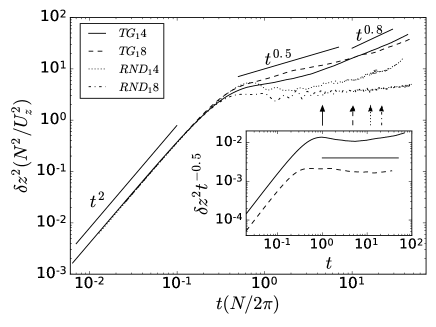
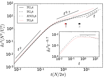
Figure 1: (Color online) Mean vertical dispersion $\delta z^{2}$ for (left) runs in cubic domains (boxes with aspect ratio 1:1), and (right) runs in elongated domains with aspect ratio 1:4, in both figures with TG and RND forcing and with different Brunt-Väisälä frequencies. The dispersion is normalized by $U_{z}^{2}/N^{2}$, the ratio of the squared mean vertical velocity to the Brunt-Väisälä frequency, and time is normalized by the Brunt-Väisälä period. Power laws are indicated as references. In each figure, the Lagrangian time of each run is indicated by a vertical arrow with the same line style as the corresponding run, while the insets show the mean vertical dispersion of some of the simulations, not normalized, and compensated by the power laws indicated in the main panels for intermediate times.

III Single-particle vertical dispersion in stably stratified turbulence

Particle dispersion in SST is inherently different from HIT as stratification suppresses vertical dispersion. As mentioned in the Introduction, linear models of SST predict the saturation of the vertical dispersion for $t\approx 2\pi/N$, as the displacement of particles is in practice vertically bounded by the stratification, resulting in an oscillatory motion of the particles Nicolleau and Vassilicos (2000). This is confirmed by numerical simulations at moderate buoyancy Reynolds number Kimura and Herring (1996); Lindborg and Brethouwer (2008).

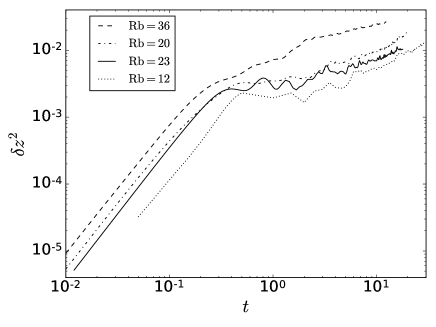
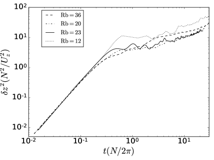
Figure 2: Mean squared vertical displacement $\delta z^{2}$ for RND runs in domains with aspect ratio 1:4 and with $N=8$ (run RND${}_{4}8$ and runs RND${}_{4}8$B to RND${}_{4}8$D, from higher to lower Re and Rb. Left: $\delta z^{2}(t)$ without normalization. Right: same, normalized by the ratio $U_{z}^{2}/N^{2}$, and with time normalized by the Brunt-Väisälä period.

We computed the single-particle vertical dispersion as $\delta z^{2}=\left<[z_{i}(t)-z_{i}(0)]^{2}\right>_{i}$, where $i$ is the particle label, and the average is computed over all particles. Figure 1 shows the resulting mean vertical dispersion in our simulations, for TG and RND forcing, different aspect ratios, and different Brunt-Väisälä frequencies (and thus, different Froude numbers). Time is normalized by $2\pi/N$ (the Brunt-Väisälä period), while $\delta z^{2}$ is normalized by $(U_{z}/N)^{2}$ (following the normalization used in Aartrijk et al. (2008)) where $U_{z}$ is, as already mentioned, the (Eulerian) r.m.s. vertical velocity in the turbulent steady state when the particles were injected in the flow (note that while $U_{z}$ does not change significantly in time and has similar values for both forcing functions, the pointwise value of $u_{z}$ changes significantly in space in the runs with TG forcing, as will be discussed in detail in Sec. IV.2). With this normalization all curves collapse from $t=0$ until $t\approx 2\pi/N$, in a time range when they display ballistic behavior $\delta z^{2}\sim t^{2}$. In Fig. 1 we also indicate with arrows the Lagrangian time $T_{L}$ of each simulation. These times are very different for each run, and are also different from the time at which the ballistic behavior ends. The end of the ballistic regime at the time of the wave period $2\pi/N$, instead of at the Lagrangian time $T_{L}$, indicates that the early-time fast vertical dispersion is dominated by the waves, in good agreement with previous studies of SST Aartrijk et al. (2008); Sujovolsky et al. (2018a): particles are first displaced ballistically by the internal gravity waves, which for $\textrm{Fr}<1$ are faster than the large-scale turbulent eddies.

The ballistic behavior observed in Fig. 1 finishes after one Brunt-Väisälä period, resulting in a change in the growth of $\delta z^{2}(t)$. In some cases (see runs RND${}_{1}4$ and RND${}_{1}8$ in Fig. 1) $\delta z^{2}(t)$ grows very slowly or even saturates at late times, displaying a plateau. The saturation was reported before in simulations of SST at moderate Re and Rb numbers Aartrijk et al. (2008); Sujovolsky et al. (2018a), where a very slow growth at late times was attributed to the effect of molecular diffusion. However, some of our runs (all TG runs even at moderate Rb, and simulations with RND forcing at higher Rb in elongated domains) display a more efficient transport (i.e., a faster growth of $\delta z^{2}(t)$ for $t>2\pi/N$) when compared with the runs that display the plateau. The enhanced dispersion after $t>2\pi/N$ seems to be controlled, at least for RND forcing, by Rb, suggesting it may be caused by turbulence generated by shear instabilities or by overturning events. As a reference, some power laws are shown in Fig. 1 in this late time regime, and the mean vertical dispersions of some of the simulations, compensated by these power laws, are shown in insets. However, note that as will be discussed in Sec. V, the enhanced dispersion seen in some of these runs is a combination of both the effects of the waves and of the turbulent eddies, and as a result it is not captured by a unique power law, and tends in some of the runs (at sufficiently high Rb or for sufficiently strong overturning events) to a $\delta z^{2}\sim t$ behavior for sufficiently long times.

To further illustrate the effect of varying Rb, Fig. 2 shows the single-particle vertical dispersion for several runs with RND forcing, and with the same parameters as RND${}_{4}8$ (runs RND${}_{4}8$B to RND${}_{4}8$D), but with different spatial resolution and values of Rb (by decreasing Re). Run RND${}_{4}8$D, with the lowest values of $\textrm{Re}\approx 300$ and of $\textrm{Rb}\approx 12$, displays a saturation in $\delta z^{2}(t)$ at $tN/(2\pi)\approx 7\times 10^{-1}$, a plateau until $tN/(2\pi)\approx 5$, and then a slow growth. As Rb increases the plateau shortens, until it completely disappears for run RND${}_{4}8$ (with $\textrm{Re}\approx 3000$ and $\textrm{Rb}\approx 36$). Note that while one panel in Fig. 2 shows $\delta z^{2}$ without any normalization (and thus the increase in its amplitude with increasing Rb can be easily appreciated), the other panel shows $\delta z^{2}(N^{2}/U_{z}^{2})$. In this latter case, the change in the amplitude seen at late times is thus associated with the fact that $U_{z}^{2}$ also increases with increasing Rb, resulting in a net decrease of $\delta z^{2}(N^{2}/U_{z}^{2})$ with increasing Rb. However, this normalization (together with the normalization of the time $t$ by the Brunt-Väisälä period) makes all curves collapse again at early times, further showing that the ballistic behavior is independent of Rb and thus of the strength of the small-scale turbulence.

The case of TG forcing is different, as the plateau in $\delta z^{2}(t)$ at intermediate times is not present even in runs at moderate Rb. Although turbulence plays an important role in the dispersion at high Rb, the TG forcing function generates a coherent large-scale flow which creates strong fronts and helps instabilities to develop Sujovolsky et al. (2018b), enhancing vertical dispersion even at values of Rb which are low when compared to the RND case. In the next section we study the gradient Richardson number Ri_g, with a special focus on the TG simulations, to characterize the features of this flow that result in differences in the vertical dispersion.

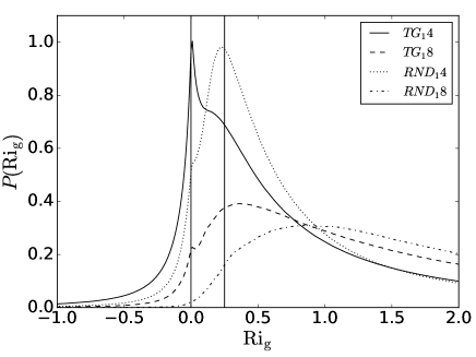
Figure 3: PDFs of the Eulerial local gradient Richardson number Ri_g, for all runs in cubic domains (runs TG${}_{1}4$ and TG${}_{1}8$ with TG forcing and $N=4$ and 8 respectively, and runs RND${}_{1}4$ and RND${}_{1}8$ with RND forcing and $N=4$ and 8 respectively). Vertical solid lines at $\textrm{Ri}_{g}=0$ and $1/4$ are shown as references.

IV The local gradient Richardson number

IV.1 General properties of the local gradient Richardson number

The local gradient Richardson number provides a measure of the vertical stability of stratified flows. When $\textrm{Ri}_{g}({\bf r})<1/4$ pointwise, local shear instabilities can take place Davidson (2013), while if $\textrm{Ri}_{g}<0$, then $\partial_{z}\theta>N$, and an overturning instability can develop generating convection locally in the flow. Figure 3 shows the probability density functions (PDFs) of the Eulerian $\textrm{Ri}_{g}$ for all runs in cubic domains. The PDFs of runs with $N=4$ (TG${}_{1}4$ and RND${}_{1}4$) display larger probabilities of low values of $\textrm{Ri}_{g}$ ($<1/4$ and $<0$) than the runs with the same forcing but with $N=8$ (TG${}_{1}8$ and RND${}_{1}8$). As $N$ is increased (for a given forcing), the peak of the PDF moves to larger values of $\textrm{Ri}_{g}$. This indicates, as expected, that as stratification increases vertical instabilities are inhibited, and as a result we can also expect a less efficient vertical transport (in agreement with the single-particle vertical dispersion observed in the previous section). However, when we compare TG and RND runs with the same value of $N$, we see that TG runs still shows larger probabilities of $\textrm{Ri}_{g}<1/4$ and of $\textrm{Ri}_{g}<0$. Indeed, the PDFs of the TG runs are shifted towards the left relative to the RND set, indicating that this flow is more vertically unstable and, consequently, can be more efficient at vertically displacing particles.

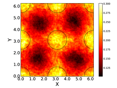
Figure 4: (Color online) Vertically averaged absolute value of the Eulerian vertical velocity, $\left<|u_{z}|\right>_{z}$, for run TG${}_{4}4$ (TG forcing, $N=4$, and aspect ratio 1:4). Bright regions correspond to large vertical velocities in absolute value. As the domain is periodic in both $x$ and $y$ directions, the regions with large $\left<|u_{z}|\right>_{z}$ can be enclosed by four circles (cylinders when extended in the $z$ direction), indicated as a reference by the black solid lines.

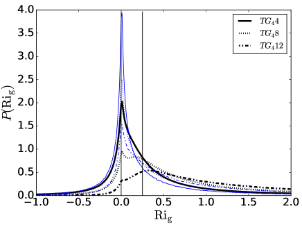
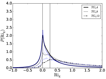
Figure 5: (Color online) Both panels show, in black thick lines, the Lagrangian PDFs of the gradient Richardson number Ri_g for TG runs in boxes with 1:4 aspect ratio. This PDF is compared with (left) the PDFs of $\textrm{Ri}_{g}$ restricted to Lagrangian velocities $|v_{z}|>\left<|v_{z}|\right>+2\sigma_{v_{z}}$ (where $\sigma_{v_{z}}$ is the dispersion in $v_{z}$) in thin (blue) lines, and (right) the PDFs of $\textrm{Ri}_{g}$ restricted to particles in the circular regions indicated in Fig. 4. Vertical lines at $\textrm{Ri}_{g}=0$ and $\text{Ri}_{g}=1/4$ are shown as references.

IV.2 The spatial structure of the local gradient Richardson number in the TG flow

We are interested in how the TG forcing affects the structure of the local gradient Richardson number. As the forcing generates a coherent large-scale flow, which in principle can affect vertical transport, we show first in Fig. 4 the mean vertical value of the absolute Eulerian vertical velocity $\left<|u_{z}|\right>_{z}$ computed for run TG${}_{4}4$ (where the subscript $z$ in the brackets indicates the average was computed along the $z$-coordinate). As explained in Sec. II, the TG flow consists of pairs of counter-rotating horizontal vortices, separated vertically by shear layers. Pressure gradients create a vertical circulation Sujovolsky et al. (2018b), and as a result the forcing generates a coherent structure at the largest scales that organize the flow into regions of high and low $\left<|u_{z}|\right>$. As a result, some well-defined spatial regions in the flow display a bias towards larger values of $|u_{z}|$ (also associated with the generation of front- and filament-like structures in the flow, as discussed in Sujovolsky et al. (2018b)). As a comparison, the runs with RND forcing do not display such a large-scale structure (not shown). It can thus be expected that Lagrangian particles approaching these regions in the TG flow will have a tendency to suffer larger displacements in the vertical direction, thus increasing $\delta z^{2}$ even at moderate Rb.

To confirm this effect, Fig. 5 shows the PDFs of the Lagrangian Ri_g (i.e., now computed using the gradients as seen by the Lagrangian particles) for runs with TG forcing in the box with 1:4 aspect ratio. Gradients (as well as velocity and density fluctuations) seen by the Lagrangian tracers are computed for each time and at each particle position using the same three-dimensional cubic spline interpolation used to integrate the particles discussed in Sec. II. From these quantities, the PDFs of Ri_g are computed. As expected, the “Lagrangian” PDFs coincide with the Eulerian PDFs, which are computed at a fixed time and for all points in the Eulerian spatial grid; however, the PDFs from Lagrangian data will allow us next to more easily compute statistics restricted to specific conditions over the fluid elements. As a result, as observed before for the Eulerian statistics, for the complete dataset as the stratification increases (i.e., for higher $N$) the mean gradient Richardson number also increases, and the fraction of fluid elements with $\textrm{Ri}_{g}<1/4$ or $\textrm{Ri}_{g}<0$ (i.e., prone to overturning) decreases. But, as we just mentioned, the computation of Ri_g using the gradients as seen by the Lagrangian particles also allow us to compute conditional statistics, e.g., only for instants when the particles suffer large vertical velocities, or when the particles are in a specific region in space. Using the mean of the absolute Lagrangian vertical velocity $\left<|v_{z}|\right>$ (averaged over all particles and over time), and the standard deviation of $v_{z}$ ($\sigma_{v_{z}}$), we computed the PDF of $\textrm{Ri}_{g}$ restricted to particles with absolute vertical velocity $2\sigma_{v_{z}}$ larger than $\left<|v_{z}|\right>$ (see Fig. 5). With this restriction, the fraction of fluid elements that can suffer overturning instabilities increases (note the PDFs have a larger peak at $\textrm{Ri}_{g}=0$, display larger values for $\textrm{Ri}_{g}<0$, and smaller values for $\textrm{Ri}_{g}>0$ when compared with the PDFs at the same $N$ without any restriction). This indicates that there is a correlation between fluid elements with $\textrm{Ri}_{g}\leq 0$ and large values of $|v_{z}|$ (and thus, of particles displacing larger distances in the vertical direction, and contributing to $\delta z^{2}$). We also see that as $N$ is increased, the probability of finding fluid elements with $\textrm{Ri}_{g}\leq 0$ decreases even when restricted to parcels with large $|v_{z}|$. Finally, Fig. 5 also shows the PDF of $\textrm{Ri}_{g}$ restricted to the instants the particles are in the spatial regions of the large-scale circulation for which the largest absolute values of $u_{z}$ were observed in Fig. 4. A similar (albeit weaker) behavior as for the restriction in $v_{z}$ is found, with the shift in the peak of the PDFs towards smaller values of $\textrm{Ri}_{g}$, confirming the relevance of the geometry of the large-scale flow in the TG runs for the vertical transport of Lagrangian particles.

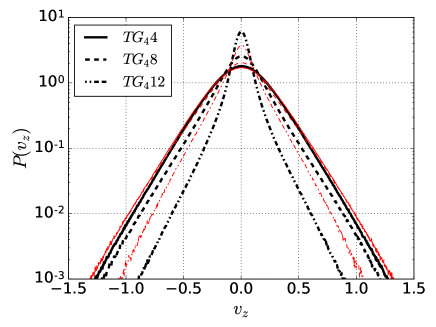
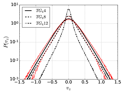
Figure 6: (Color online) Both panels show in thick black lines the PDFs of the Lagrangian vertical velocity $v_{z}$ for TG runs in domains with 1:4 aspect ratio and varying $N$. PDFs restricted to particles in instants with $\textrm{Ri}_{g}<1/4$ (left), or with $\textrm{Ri}_{g}<0$ (right), for the same runs, are shown in (red) thin lines.

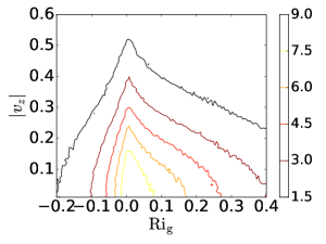
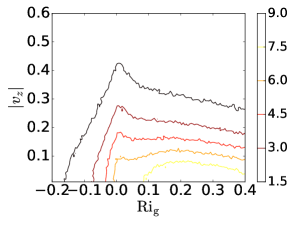
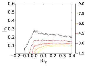
Figure 7: (Color online) Isocontours of the joint probability distribution function of $\textrm{Ri}_{g}$ and $|v_{z}|$, $P(\textrm{Ri}_{g},|v_{z}|)$, for runs TG${}_{4}4$ (left), TG${}_{4}8$ (middle), and TG${}_{4}12$ (right).

To further study the effect of $\textrm{Ri}_{g}$ on the vertical velocity of the particles, Fig. 6 shows the PDFs of the Lagrangian vertical velocity for all particles in TG runs with aspect ratio 1:4 and with varying $N$. As previously reported in Rorai et al. (2014); Feraco et al. (2018), the vertical velocity does not follow Gaussian statistics, and display strong tails (this feature is not exclusively associated with the TG forcing, as the same behavior was found in simulations with random forcing, see Rorai et al. (2014)). In Feraco et al. (2018) the extreme values were shown to be associated to intermittent overturning instabilities in the flow. Note that the behavior reported in Feraco et al. (2018) is non-monotonous in Fr, although for sufficiently small Fr (or sufficiently large values of $N$) the maximum values of $v_{z}$ decrease with increasing stratification (see Fig. 6). When we compute the PDFs restricted to particles in instants for which $\textrm{Ri}_{g}<1/4$ or $\textrm{Ri}_{g}<0$, while for the runs with moderate stratification ($N=4$ and 8) there are only small changes in the tails of the PDFs (albeit extreme values of $v_{z}$ become more probable), for stronger stratification ($N=12$) the changes are significantly larger, with stronger tails. This further confirms that points with $\textrm{Ri}_{g}<1/4$ or $\textrm{Ri}_{g}<0$ are associated with larger values of $v_{z}$, and can thus be expected to be associated with the enhanced dispersion after $t>2\pi/N$ at least in the TG runs.

This can be also confirmed in Fig. 7, which shows the joint probability density function as a function of $\textrm{Ri}_{g}$ and $|v_{z}|$, $P(\textrm{Ri}_{g},|v_{z}|)$, for the TG runs with aspect ratio 1:4 and with varying $N$. As the stratification increases, the probability of finding particles with large values of $|v_{z}|$ decreases, while that of finding larger values of $\textrm{Ri}_{g}$ increases. For $N=4$ and $N=8$ note the correlation between larger absolute values of the vertical velocity with $\textrm{Ri}_{g}\approx 0$ values, which is significantly weaker in the run with $N=12$.

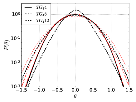
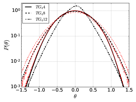
Figure 8: (Color online) PDFs of $\theta$ as seen by the Lagrangian particles (thick black curves), and the same PDFs restricted (in thin red curves) to (left) particles at times with $\textrm{Ri}_{g}<1/4$, and (right) particles at times with $\textrm{Ri}_{g}<0$. Except for the run TG${}_{4}12$, all PDFs are compatible with Gaussian statistics for $\theta$.

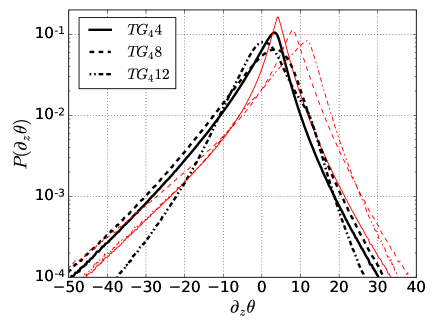
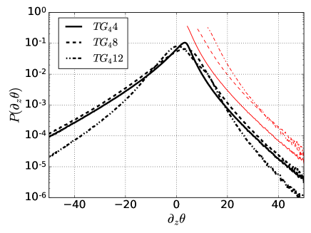
Figure 9: (Color online) PDFs of the Lagrangian vertical temperature gradients $\partial_{z}\theta$ (thick black curves), and the same PDFs restricted (in thin red curves) to (left) $\textrm{Ri}_{g}<1/4$ and (right) $\textrm{Ri}_{g}<0$.

Finally, we also studied how the value of $\textrm{Ri}_{g}$ affects $\theta$ and $\partial_{z}\theta$ with increasing stratification (note that the local value of $\partial_{z}\theta$ is important for overturning instabilities, as the gradient of the buoyancy fluctuations can compete with the background gradient, resulting in local inversion of the stratification). Figure 8 shows the PDFs of $\theta$ as seen by the Lagrangian particles, and the same PDFs restricted to instants when $\textrm{Ri}_{g}<1/4$ or $\textrm{Ri}_{g}<0$, in all cases for the $TG_{4}$ runs. For $N=4$ the PDFs of $\theta$ are close to Gaussian, and the restriction in the values of $\textrm{Ri}_{g}$ has a negligible effect in the statistics. However, for $N=8$, while the PDFs are still close to Gaussian, the restricted PDFs show a lower probability for $|\theta|<0.5$ and higher probability for $|\theta|>0.5$, indicating particles with $\textrm{Ri}_{g}<1/4$ or $\textrm{Ri}_{g}<0$ are more likely to be found in points with higher potential energy density $\sim\theta^{2}$. This behavior is enhanced for $N=12$, for which the PDFs also display non-Gaussian tails. Finally, Fig. 9 shows the PDFs of the Lagrangian vertical gradients of $\theta$, $\partial_{z}\theta$, which are non-Gaussian and asymmetric. The asymmetry is enhanced when the PDFs are restricted to instants when $\mathrm{Ri_{g}}<1/4$ or $\mathrm{Ri_{g}}<0$. While the non-restricted PDFs have their maximum at $\partial_{z}\theta\gtrsim 0$, for the restricted PDFs the maximum is at $\partial_{z}\theta\approx N$. From the ideal Boussinesq equation for $\theta$ (Eq. 2, with $\kappa=0$), it can be seen that ${\boldsymbol{\nabla}}\theta=\left(0,0,N\right)$ is a fixed point of both the equations for $\theta$ and for the Lagrangian evolution of $\partial_{z}\theta$, which could explain the accumulation of (restricted) particles with $\partial_{z}\theta\approx N$. Also, at points where $\mathrm{Ri_{g}}<0$, then $\partial_{z}\theta>N$ (for which overturning events can occur). This is the reason why the PDFs of particles restricted to $\mathrm{Ri_{g}}<0$ in Fig. 9 only take values of $\partial_{z}\theta$ greater than $N$. Finally, note that since $\textrm{Ri}_{g}$ depends explicitly on $\partial_{z}\theta$ and not on the pointwise value of $\theta$, a restriction on the values of $\textrm{Ri}_{g}$ can be expected to affect the PDFs in Fig. 9 more strongly than those in Fig. 8, as is indeed observed in the figures.

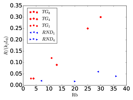
Figure 10: (Color online) Overturning probability normalized by the forcing wave number and unit length, $R/(k_{f}L_{0})$, as a function of the Reynolds Buoyancy number Rb for all simulation in table 1.

IV.3 Overturning probability and the buoyancy Reynolds number

As already mentioned, the extreme vertical velocities reported in the previous subsection are not exclusive of the TG flow. In Rorai et al. (2014); Feraco et al. (2018), non-Gaussian PDFs of $u_{z}$, $v_{z}$, and $\theta$ were reported for RND forcing depending on the values of Fr and Rb. However, it is clear from the results shown so far that the geometry of the TG flow facilitates the development of overturning instabilities and the occurrence of extreme values of the vertical velocity even at moderate Rb.

In the next section we will use these results to build a simple model for single-particle vertical dispersion, for all cases considered and independently of the two specific forcing function used. The results in Sec. III suggest that while the ballistic behavior of $\delta z^{2}$ for $t<2\pi/N$ is dominated by the waves, the differences in $\delta z^{2}$ for $t>2\pi/N$ depend on the strength of the vertical velocity and of the turbulence. For moderate turbulence (i.e., moderate values of Rb) and without a large-scale vertical circulation, $\delta z^{2}$ is dominated by the waves even at late times, resulting in the observed saturation of the single-particle vertical dispersion. But for larger values of Rb (as in some of the RND runs), or in the presence of a large-scale flow (as in all TG runs), strong vertical updrafts or downdrafts can enhance vertical transport resulting in the growth of $\delta z^{2}$ at late times. We will measure the probability of this happening by introducing an overturning probability $R$, defined as the fraction of particles (in the Lagrangian frame) or the fraction of space volume (in the Eulerian frame) with $\textrm{Ri}_{g}<0$. Figure 10 (see also table 1) gives $R/(k_{f}L_{0})$ as a function of Rb for all runs, where $R$ is measured as the integral of the PDF of $\textrm{Ri}_{g}$ for $\textrm{Ri}_{g}<0$. The normalization of $R$ by the product $k_{f}L_{0}$ (where $k_{f}$ is the forcing wave number and $L_{0}$ the unit length) makes all simulations with a given forcing (either RND or TG) collapse in the vicinity of approximate linear relations independently of the forcing wave number used. Indeed, the data follows (for the range of Rb considered) a linear relation with Rb, with two different slopes for the TG and RND runs (even when the runs in each set also have different aspect ratios, forcing wavenumbers, Reynolds, and Froude numbers). As expected, for fixed Rb, the TG runs display larger values of $R$ than the RND runs.

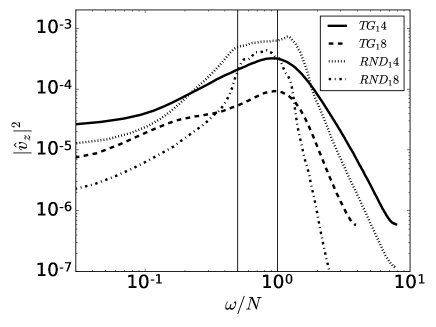
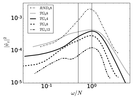
Figure 11: Power spectrum of the Lagrangian vertical velocity for (left) runs in cubic domains, and (right) runs in elongated domains. Frequencies have been normalized by the Brunt-Väisälä frequency. The solid vertical lines indicate (from left to right) $\omega=N/2$ and $\omega=N$.

V Single-particle vertical dispersion model

To study the vertical dispersion of single-particles observed in the DNSs of SST in section III, we now present a stochastic model that combines a random wave model (to consider the effect of internal gravity waves) with a CTRW Rast et al. (2016) (to capture the effect of overturning by turbulent or large-scale eddies).

Based on the results presented so far (and in particular, on the observation that at early times the behavior is dominated by waves), the wave model we present consists of a sum of linear waves with random phases. The presence of internal gravity waves in these flows, and their dispersion relation, have been studied before in spatio-temporal studies (see, e.g., Clark di Leoni and Mininni (2015)), further indicating their relevance in the dynamics of SST. We can thus approximate the trajectory of a Lagrangian particle moving vertically following these waves as

$$z_{wav}(t)=\Re\left[{\sum_{\omega}A_{\omega}e^{i(\omega t+\phi_{\omega})}}\right],$$ (13)

where $\phi_{\omega}$ is a random phase (note that as we are interested only in the vertical motion of the particles, the possible dependence of travelling waves on $x$ and $y$ can be ignored or absorbed into the random phase), and where the sum is performed over $N_{\omega}$ uniformly distributed frequencies in the range of frequencies $\omega\in[\omega_{min},\omega_{max}]$. The amplitude of the waves satisfies the spectral relation

$$A_{\omega}=A_{0}\,\omega^{-1},$$ (14)

for the same range of frequencies, and where $A_{0}$ is a normalization factor. The dependence of $A_{\omega}\sim\omega^{-1}$ follows from observations that the power spectrum of the actual Lagrangian vertical velocity has a broad maximum with approximately constant amplitude near the Brunt-Väisälä frequency. Note that associating $v_{z}$ with $\dot{z}_{wav}=\Re[{\sum A_{\omega}\omega e^{i(\omega t+\phi_{\omega})}}]$, a flat power spectrum for $v_{z}$ implies Eq. (14) for the amplitude of the waves. Once $N_{\omega}$ is chosen, the normalization factor $A_{0}$ can then be fixed as $A_{0}=\left(2U_{z}^{2}/N_{\omega}\right)^{1/2}$ by imposing that for each particle $\left<\dot{z}_{wav}^{2}\right>_{t}$ (averaged over time) must be equal to the mean squared Eulerian vertical velocity $U_{z}^{2}$ (also equal to the mean squared Lagrangian vertical velocity) using Parseval’s theorem.

Note also that a flat Lagrangian spectrum for a range of frequencies is compatible with oceanic observations of the so-called Garrett-Munk spectrum, and also with numerical simulations of SST Sujovolsky et al. (2018a). As an example, Fig. 11 shows the power spectrum of the Lagrangian vertical velocity for all runs in table 1. There is a broad peak near $\omega=N$, and in several of the runs an approximately flat spectrum can be observed in its vicinity (as a reference, the figure indicates a range of frequencies $[N/2,N]$), with a decay compatible with a power law for $\omega>N$, and a slowly decaying, or almost flat, spectrum for $\omega\ll N$). Also, for the runs with the smallest values of Rb considered in this study (runs TG${}_{1}8$ with $\textrm{Rb}=3.2$, and TG${}_{4}12$ with $\textrm{Rb}=4.3$), a secondary peak at smaller frequencies can be observed. In these runs turbulence is moderate, and the waves dominate the dispersion at intermediate times.

As the dispersion relation of internal gravity waves is $\omega=Nk_{\perp}/k\leq N$, we set $\omega_{max}=N$, and for simplicity, from the results in Fig. 11 we set $\omega_{min}=N/2$ in all cases. It then follows from Eq. (13) that the vertical displacement of any particle following the waves is given by

$$\delta z_{wav}(t)=z_{wav}(t)-z_{wav}(0)=\sum_{\omega}A_{w}\left[\cos(\omega t+\phi_{\omega})-\cos(\phi_{\omega})\right].$$ (15)

The square of this expression, when averaged over an ensemble of particles and waves, can be approximated by (see Appendix A)

$$\left<\delta z_{wav}^{2}\right>(t)=\left\{\begin{array}[]{lcc}U_{z}^{2}t^{2}&\textrm{if}&t\leq N^{-1},\\ \\ Q(t)&\textrm{if}&N^{-1}<t<4N^{-1},\\ \\ \dfrac{4U_{z}^{2}}{N^{2}}&\textrm{if}&t\geq 4N^{-1},\end{array}\right.$$ (16)

where $Q(t)$ is a third order polynomial function obtained by imposing $\left<\delta z_{wav}^{2}\right>$ and its time derivative to be continuous in time (see Appendix A). Figure 12 shows the mean dispersion for many particles calculated from a stochastic superposition of waves as in Eq. (15), and from the function in Eq. (16), in both cases using values of $A_{0}$ and $N$ that adjust the vertical r.m.s. velocity and the Brunt-Väisälä frequency of several TG runs. The function in Eq. (16) is in good agreement with the sum of random waves, specially for short and long times. Note also that this simple model based on a superposition of waves captures the early-time ballistic behavior of $\delta z^{2}\sim t^{2}$ seen for all DNSs in Fig. 1, as well as the saturation at late times seen in Fig. 1 for some of the simulations.

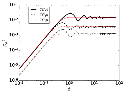
Figure 12: (Color online) Mean dispersion obtained from a random superposition of waves as in Eq. (15) (in thick black lines), and from Eq. (16) (in thin red lines), with the parameter $A_{0}$ to match the Eulerian vertical r.m.s. velocity and $N$ the Brunt-Väisälä frequency for some of the TG runs (see labels in the inset).

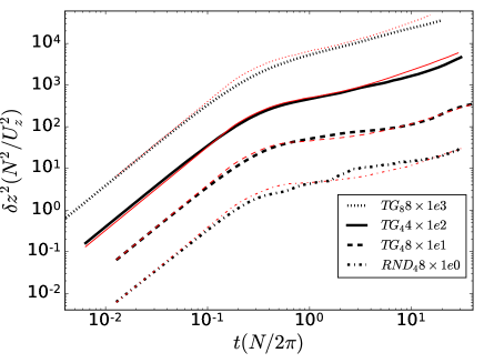
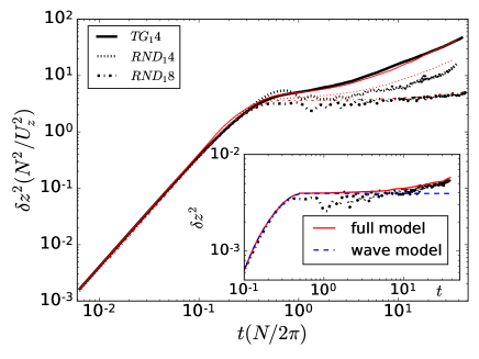
Figure 13: (Color online) Mean vertical dispersion $\delta z^{2}$ for (left) runs in elongated domains with amplitudes rescaled for better visualization (see the inset), and (right) runs in cubic domains, for RND and TG forcing, and with different values of $N$. Normalizations of $\delta z^{2}$ and of time are the same as in Fig. 1. In both figures the thick (black) lines show the results from the DNSs, and the thin (red) lines show the results obtained from the single-particle dispersion model. The inset on the right shows a detail of $\delta z^{2}$ for run RND${}_{1}8$ (thick dash-dotted curve), together with the mean squared vertical displacement predicted by the full model, and by the superposition of random waves alone.

The behavior shown in Fig. 12 is similar to the vertical dispersion predicted for SST by other models based on a linear superposition of waves Nicolleau and Vassilicos (2000), and is reminiscent of the vertical dispersion observed in previous DNSs of SST at moderate values of Rb Aartrijk et al. (2008); Sujovolsky et al. (2018a). However, this wave model fails to reproduce the dispersion observed at long times in some of our runs. To introduce an enhanced vertical dispersion by turbulent overturning, we add a CTRW model that mimics the trapping of particles by eddies, resulting in vertical displacements when the flow becomes unstable such that the total vertical dispersion will be $\delta z(t)=\delta z_{wav}(t)+\delta z_{CTRW}(t)$.

To compute $\delta z_{CTRW}(t)$, in each step $t$ of the random walk process we assume a particle has a probability $R$ of being trapped for a time $t_{t}$ inside an eddy of radius $r_{t}$ with velocity $U_{t}$. As in the previous section, $R$ is the probability of finding particles with $\textrm{Ri}_{g}<0$. Whether at a given step $t$ the particle is trapped or not is a binary decision, and thus the probability of the particle not being trapped is $1-R$ (in which case the particle does not move following eddies). When trapped, the probability of being advected by an eddy of radius $r_{t}$ is given by a Kolmogorov distribution $P(r_{t})\sim r_{t}^{4/3}$ for $r<L_{oz}$, compatible with an isotropic energy spectrum $\sim k^{-5/3}$ for wavenumbers $k>k_{oz}$; in other words, we assume that the eddies responsible for the vertical dispersion at late times are associated with overturning instabilities in the turbulent inertial range for scales equal to or smaller than the Ozmidov scale. The distribution of trapping times $P(t_{t})$ is continuous and uniform between $t_{t}=0$ and the Eulerian turnover time at the Ozmidov scale $\tau_{oz}$. Finally, at each step $t$ and if the particle is trapped, the particle velocity (or equivalently, the characteristic velocity of the eddy trapping the particle) is $U_{t}$, given by a probability distribution $P(U_{t})$ that is obtained from the observed PDF of the absolute value of the Eulerian vertical velocity (which, in practice, can be very well approximated by assuming that it follows a Rayleigh distribution, so knowledge of the r.m.s. value of $u_{z}$, $U_{z}$, is sufficient to estimate $P(U_{t})$).

As mentioned above, in each step of the CTRW if a particle is not trapped by an eddy, $\delta z_{CTRW}(t)$ will remain constant (i.e., the particle will not move as a result of eddy trapping). If it gets trapped, it will be displaced along a circle as the result of the trapping, with a vertical displacement of $r_{t}\sin(\theta_{t})$ which is just the projection of the circular trajectory of radius $r_{t}$ in the $z$ direction, and where $\theta_{t}=U_{t}t_{r}/r_{t}$ is the angle of the arc traveled during the time $t_{r}$. Thus, the random walk process just mimics in a simplified way the eventual presence of vertical eddies that can result in upward or downward transport of the Lagrangian particles. As described above the model has no free parameters; all parameters are obtained from Eulerian characteristic lengths and time scales of the flow.

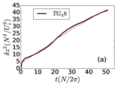
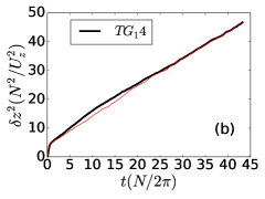
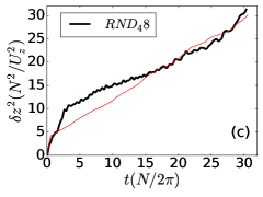
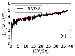
Figure 14: (Color online) Mean squared vertical displacement $\delta z^{2}$ in linear scale, for four cases: (a) TG${}_{4}8$, (b) TG${}_{1}4$, (c) RND${}_{4}8$, and (d) RND${}_{1}8$. The four cases are illustrative of runs with TG or RND forcing, with different levels of stratification, and with different domain aspect ratios. The thick (black) curves show the results from the DNSs, while the thin (red) lines show the results obtained from the model. In spite of the randomness in the DNSs and in the CTRW model, all cases display a reasonable agreement.

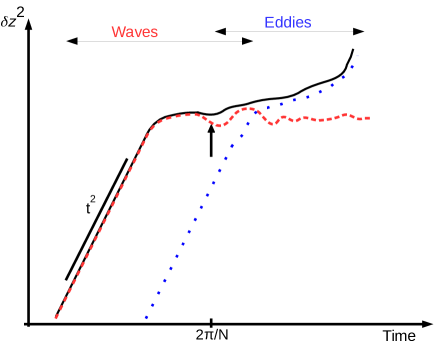
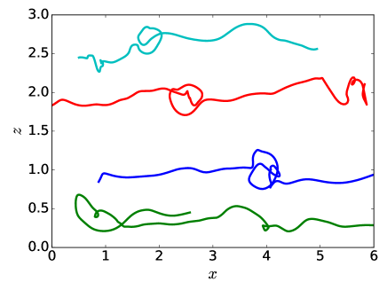
Figure 15: (Color online) Left: Sketch of the two contributions to vertical dispersion in the model. The random superposition of waves dominates at early times (red dashed curve), while the effect of turbulent eddies and overturning events become relevant at late times (blue dotted curve). The total vertical dispersion (black solid curve) results from the superposition of both effects. Right: A few particle trajectories from the TG${}_{4}4$ run projected on the $x$-$z$ plane. Note the small and wavy particles’ displacements in the vertical directions, interrupted by sudden and close to circular trajectories that result in a larger vertical displacement, which we associate by trapping by overturning eddies (see Sec. V for details).

We can summarize the computation of the entire model as follows:

1. Wave model: At any time, each particle vertical trajectory is computed as the sum of $N_{\omega}$ harmonic motions, each with amplitude $2U_{z}^{2}/(N_{w}\omega)$, and with uniformly distributed random frequencies $\omega$ between $N/2$ and $N$.

2. CTRW model:

   1. At each step $t$, a particle is trapped by and eddy with probability $R$ (or not trapped, with probability $1-R$).

   2. If the particle is trapped:

      1. The characteristic velocity of the eddy $U_{t}$ is given by $P(U_{t})$, a Rayleigh probability distribution with its mean given by the mean Eulerian vertical velocity of the flow.

      2. The eddy radius $r_{t}$ is chosen with a probability distribution $P(r_{t})\sim r^{4/3}$ for $r_{t}\leq L_{oz}$, $P(r_{t})=0$ in other case.

      3. The trapping time $t_{t}$ is chosen from a uniform probability distribution $P(t_{t})$ between 0 and $\tau_{oz}$.

      4. The central angle subtended by the arc traveled by the particle during the trapping time is computed as $\theta_{t}=U_{t}t_{t}/r_{t}$.

      5. The vertical displacement after the time $t_{t}$ is finally computed as $r_{t}\sin(\theta_{t})$.

   3. If the particle is not trapped, the particle is not displaced.

   4. The final vertical displacement resulting from the CTRW for any given particle and at a given time $t=\sum_{t=1}^{n}t_{t}$, is the sum over the $n$ vertical displacements.

3. Full model: At any given time, the total vertical displacement is obtained as the sum of the displacements generated by the waves and by the CTRW process.

The key parameters of the full model then are $N$, $U_{z}$, $L_{oz}$, and $R$, from which all other variables and probability distributions (as well as the total displacements) can be computed.

Figure 13 shows the mean vertical dispersion obtained from several DNSs, and $\delta z^{2}(t)=[\delta z_{wav}(t)+\delta z_{CTRW}(t)]^{2}$ as obtained from the wave and CTRW model (i.e., the full model). For the runs in elongated domains (with TG forcing, or larger values of Rb), as the dispersion is very similar for all runs, we rescaled $\delta z^{2}$ using an arbitrary value (indicated in the figure inset), so the curves can be distinguished more easily. In the other cases, the same normalization as in Fig. 1 was used for $\delta z^{2}$ and time. The model is in good agreement with the DNS data in all cases, and captures early and late time behavior independently of the forcing function (TG or RND), as well as cases with saturation of $\delta z^{2}(t)$ for $t>2\pi/N$ as cases in which $\delta z^{2}(t)$ keeps growing at late times. The inset in Fig. 13 shows a detail of the mean vertical dispersion for run $\textrm{RND}_{1}8$ (RND forcing with $N=8$), for which $\delta z^{2}$ almost completely saturates after $t(N/2\pi)\approx 1$, and grows only very slowly at late times. For this case, the inset also shows $\delta z^{2}$ obtained from the wave model alone (i.e., $\delta z_{wav}^{2}$), as well as $\delta z^{2}$ obtained from the full model). This case confirms that while the wave model can capture the saturation, the departure from this saturation and the growth observed at late times can only be captured if trapping by eddies is taken into account.

As mentioned in Sec. III, the aparent power laws observed at intermediate times in Fig. 1 are the result of this competition between dispersion by waves and eddies, and for sufficiently long times $\delta z^{2}$ approaches a linear $\sim t$ behavior if overturning is strong enough. To illustrate this, and to show the agreement between the model and the DNSs in more detail, Fig. 14 shows $\delta z^{2}(t)$ in linear scale for four selected runs (corresponding to cases with TG or RND forcing, with different Brunt-Väisälä frequencies, and with different domain aspect rations). Considering the inherent randomness of the DNSs results and of the CTRW process, a reasonable agreement is seen in all cases.

The differences between the early and late time behavior can now be further clarified using the model (see Fig. 15). At early times, the waves dominate the dispersion resulting in the observed ballistic regime up to the period of the slowest waves, $t\lesssim 2\pi/N$, for which the largest “fast” displacements (on the time scale of the waves) can take place. If considered alone, trapping by turbulent eddies in the CTRW model would also result in ballistic growth of $\delta z^{2}$, but it has an initial value significantly smaller, and as a result this process is subdominant to the dispersion by the waves. At intermediate times ($t\approx 2\pi/N$) dispersion by the waves saturates generating the plateau. If turbulence is moderate (and thus $R$ is also moderate), trapping by eddies is inefficient, resulting in a temporary saturation of the dispersion, or, in the most extreme cases, in a complete saturation of $\delta z^{2}$. Depending on how strong the turbulence is, at a certain time overturning events can start enhancing the dispersion, and for longer times the turbulence dominates the dynamic surpassing the effect of the waves. Remarkably, this simple picture is also compatible with the trajectories of individual Lagrangian particles. Figure 15 also shows as an example four trajectories projected into the $x$-$z$ plane, for four Eulerian eddy turn-over, and for run $\textrm{TG}_{4}4$. Small and wavy displacements can be seen in the vertical direction, interrupted by sudden and close to circular trajectories associated to trapping by overturning eddies, and which result in larger vertical displacements.

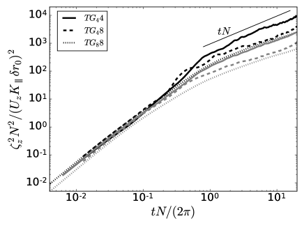
Figure 16: (Color online). Left: two-particle vertical dispersion for particles with initial vertical separation $\delta z_{0}\ll\eta$, and two initial horizontal separations: $\delta r_{0}=\eta$ (black lines) $\delta r_{0}=2\eta$ (gray lines). Results from three simulations with TG forcing are shown. The vertical dispersion was normalized by $(wK_{\parallel}\delta r_{0})^{2}/N^{2}$, and time by $1/N$. With this normalization all curves collapse during the ballistic regime. A power law at later times is indicated as a reference. Right: two-particle vertical dispersion from DNSs with RND or TG forcing (thick lines), and from the model (thin lines). The amplitude of the curves have been rescaled for better visualization (see the rescaling factor in the inset).

VI Two-particle vertical dispersion

We can also study the two-particle vertical dispersion $\zeta_{z}^{2}$, which the two simple processes presented above (dispersion by a random superposition of waves, and a CTRW process to capture the effect of turbulent overturning events) can also model. The two-particle vertical dispersion is defined as $\zeta_{z}^{2}=\langle[z_{i}(t)-z_{j}(t)]^{2}\rangle_{(i,j)}$, where $i\neq j$ are the labels of two particles that at the initial time have a vertical separation $\delta z_{0}$ and a horizontal separation $\delta r_{0}$, and where the subindex $(i,j)$ denotes that the average is computed over pairs of particles. Figure 16 shows the resulting two-particle vertical dispersion for runs TG${}_{4}4$, TG${}_{4}8$, and TG${}_{8}8$. We consider pairs of particles which at time $t=0$ have a vertical separation $\delta z_{0}\ll\eta$ (where $\eta$ is the Kolmogorov dissipation scale), and horizontal separations $\delta r_{0}\approx\eta$ or $\delta r_{0}\approx 2\eta$ (see Aartrijk et al. (2008) for a detailed study on different choices of the initial separation in two-particle dispersion in SST). Normalizing the vertical dispersion $\zeta_{z}^{2}$ by $(U_{z}K_{\parallel}\delta r_{0})^{2}/N^{2}$ all curves approximately collapse during the ballistic regime. As for the case of single-particle dispersion, we see again a growth of the two-particle dispersion at late times, which is linear or almost linear with $t$ in all runs. Here we also see an effect of Rb: simulations with larger Rb display larger two-particle vertical dispersions at late times. It is also worth pointing out that when the initial horizontal separation $\delta r_{0}$ is increased (for a given run), the short-time two-particle dispersion augments proportionally, but the late-time two-particle dispersion remains equal, indicating a decorrelation of the two particles at late times as reported before in Aartrijk et al. (2008) (note that in Fig. 16, as $\zeta_{z}^{2}$ is normalized by $\delta r_{0}^{2}$, this late-time decorrelation results in different amplitudes of $(\zeta_{z}/\delta r_{0})^{2}$ as $\delta r_{0}^{2}$ is changed).

As mentioned above, the two-particle vertical dispersion can be modeled using an extension of the single-particle model. As before, we consider the effect of the waves and of the turbulent eddies separately. First, if we have two particles which are initially very close to each other (almost at the same height, but with a horizontal displacement $\delta r_{0}$), we can assume they will be displaced by the same waves but with a phase difference between the two (for each wave with frequency $\omega$) given by

$$\phi^{\prime}_{\omega}\approx\phi_{\omega}+k\,\delta r_{0}.$$ (17)

Here $\phi_{\omega}$ is the phase of the wave seen by one of the particles, $\phi^{\prime}_{\omega}$ is the phase seen by the other particle, $k$ is the wavenumber, and we approximate the total separation between the two particles by $\delta r_{0}$ (as $\delta z_{0}\ll\eta$). Using the expressions for the displacements of a particle in a superposition of random waves given by Eqs. (13) and (15), we can estimate the separation as a function of time for a single pair as

$$\zeta_{ij,(wav)}(t)=\sum_{\omega}A_{\omega}\left\{\left[\cos(\omega t+\phi_{\omega})-\cos(\phi_{\omega})\right]-\left[\cos(\omega t+\phi^{\prime}_{\omega})-\cos(\phi^{\prime}_{\omega})\right]\right\}+\delta z_{0},$$ (18)

where the subindices $i$ and $j$ again label the pairs of particles that at the initial time meet the condition $\delta r_{0}\approx\eta$ (or $\approx 2\eta$). Equation (18) is just the difference between two single-particle vertical trajectories, to which we added an initial vertical separation $\delta z_{0}\ll\eta$. As we did in the previous section, the resulting dispersion, when averaged over several pairs of particles and sets of random waves, can be approximated as (see Appendix B)

$$\left<\zeta_{z,(wav)}^{2}\right>(t)\approx\left\{\begin{array}[]{lcc}U_{z}^{2}\left(2.1\delta r_{0}\dfrac{2\pi}{L_{\parallel}}\right)^{2}t^{2}&\textrm{if}&t<N^{-1},\\ \\ Q_{2}(t)&\textrm{if}&N^{-1}<t<4N^{-1},\\ \\ \dfrac{16U_{z}^{2}(2.1\delta r_{0}\pi)^{2}}{\left(L_{\parallel}N\right)^{2}}&\textrm{if}&t\geq 4N^{-1},\end{array}\right.$$ (19)

where, as in the single-particle approximation in Eq. (16), $Q_{2}(t)$ is a third order polynomial interpolation for the two-particle case obtained by imposing the function and its derivative to be continuous in time, and we neglected all terms in $\delta{{z}_{0}}$ and $\delta{{z}_{0}}^{2}$ as they are small when compared with the leading order terms.

As at late times the particles separate significantly from each other, to take into account the effect of overturning we can assume the two particles are uncorrelated, and as a result we can just consider two independent CTRW processes with the same properties as the one described in the previous section for single-particles, one for each particle in the pair. This is compatible with observations of two-particle dispersion in DNSs of SST Aartrijk et al. (2008), and with the results from DNSs shown above, indicating the late time dispersion becomes independent of the original separation $\delta r_{0}$. The final result of combining $\zeta_{z,(wav)}$ with the CTRW processes is shown in Fig. 16. The model is in good agreement with the two-particle vertical dispersion obtained from the DNSs, both in the ballistic regime as well as for long times when dispersion becomes dominated by the turbulent eddies, for both forcing functions considered, different domain aspect ratios, and different values of Fr and Rb.

VII Conclusions

In this paper we studied single- and two-particle vertical dispersion for Lagrangian trajectories in forced stably stratified turbulence, using two different forcing functions (Taylor-Green and random forcing), domains with different aspect ratios, and different Froude and Reynolds numbers. Using direct numerical simulations we showed that late-time saturation of single-particle vertical dispersion, reported in previous studies of this problem, is obtained only for moderate values of the buoyancy Reynolds number, and that for larger values of Rb, or even for moderate Rb in the case of the Taylor-Green flow that develops a vertical circulation, the saturation does not take place. Instead, $\delta z^{2}$ keeps growing in time after the ballistic regime, albeit at a slower rate than in homogeneous and isotropic turbulence.

We showed that the gradient Richardson number plays an important role in the strength of the vertical transport of Lagrangian tracers, as overturning fluid elements with $\textrm{Ri}_{g}<0$ give an important contribution to vertical displacement of Lagrangian particles. In particular, regions of the flows with higher vertical velocity present a higher probability of having particles with $\textrm{Ri}_{g}<0$ and vice versa. The joint probability (or restricted PDFs) between $\textrm{Ri}_{g}$ and the Lagrangian vertical velocity, temperature fluctuations and gradients were studied, confirming this correlation.

Based on these results, we derived models for single- and two-particle vertical dispersion that consist of a superposition of random waves (to capture the early time ballistic regime), and an eddy-constrained continuous-time random walk process (to capture the effect of turbulent eddies and overturning instabilities in the flow at late times). These models, together with the model for single-particle horizontal dispersion in Sujovolsky et al. (2018a), provide a description for the anisotropic dispersion in both the vertical and horizontal directions of stably stratified turbulence. The vertical dispersion obtained from the model presented here is in good agreement with the vertical dispersions obtained from the direct numerical simulations. This agreement strengthens the observation that the waves dominate the dynamic of particles at short times, resulting in the initial ballistic regime, while at intermediate times ($t\approx 2\pi/N$) linear and non-linear effects coexist in the dynamics, giving rise to a transient that can develop (or not) a plateau on the dispersion depending on how strong (or weak) is the effect of overturning events. At later times, and if turbulence is sufficiently strong (as measured by Rb, or equivalently, by the probability of a fluid element to suffer overturning, $R=P(\textrm{Ri}_{g}<0)$), turbulence (modeled here by the continuous-time random walk process) dominates. The superposition of linear and turbulent contributions to the dispersion in the model thus allows clarification of the relevant time and length scales involved in the dynamics of Lagrangian tracers in stratified turbulence. Finally, as all parameters in the model can be obtained from large-scale Eulerian properties of the flow, the model opens the door to modeling turbulent dispersion of tracers in Eulerian simulations of stratified flows that do not resolve the smallest scales in the flow, as usually is the case in the study of atmospheric and oceanic flows.

Appendix A Derivation of the single-particle dispersion wave model

We want to derive averaged expressions for the dispersion as a function of time resulting from a random superposition of waves as that given by Eq. (15). For short times, from

$$\delta z_{wav}(t)=\sum_{\omega}A_{w}\left[\cos(\omega t+\phi_{\omega})-\cos(\phi_{\omega})\right],$$ (20)

we can take the square, use the trigonometric identity $\cos(\omega t+\phi_{\omega})=\cos(\omega t)\cos(\phi_{\omega})-\sin(\omega t)\sin(\phi_{\omega})$, the Taylor expansions to first order $\sin(\omega t)\approx\omega t$ and $\cos(\omega t)\approx 1$, and Eq. (14) with $A_{0}=(2U_{z}^{2}/N_{\omega})^{1/2}$, to get

$$\delta z^{2}_{wav}\approx t^{2}\dfrac{2U_{z}^{2}}{N_{\omega}}\left[\sum_{\omega}\sin(\phi_{\omega})\right]\left[\sum_{\omega^{\prime}}\sin(\phi_{\omega^{\prime}})\right]=t^{2}\dfrac{2U_{z}^{2}}{N_{\omega}}\left[\sum_{\omega}\sin^{2}(\phi_{\omega})+\sum_{\omega,\omega^{\prime}\neq\omega}\sin(\phi_{\omega})\sin(\phi_{\omega^{\prime}})\right].$$ (21)

As the average over random phases $\phi$ uniformly distributed between $0$ and $2\pi$ is

$$\left<\sin(\phi)\right>_{\phi}=\left<\cos(\phi)\right>_{\phi} = 0,$$ (22)

$$\left<\sin^{2}(\phi)\right>_{\phi}=\left<\cos^{2}(\phi)\right>_{\phi} = 1/2,$$ (23)

for $\phi_{\omega}$ and $\phi_{\omega^{\prime}}$ two independent stochastic variables, for short times and after averaging over an ensemble of particles with different sets of random waves, we then have

$$\left<\delta z^{2}_{wav}\right>(t)\approx t^{2}U_{z}^{2}.$$ (24)

For long times

$$\delta z_{wav}^{2}(t)=\dfrac{2U_{z}^{2}}{N_{\omega}}\left\{\sum_{\omega}\dfrac{1}{\omega}\left[\cos(\omega t+\phi_{\omega})-\cos(\phi_{\omega})\right]\right\}\left\{\sum_{\omega^{\prime}}\dfrac{1}{\omega^{\prime}}\left[\cos(\omega^{\prime}t+\phi_{\omega^{\prime}})-\cos(\phi_{\omega^{\prime}})\right]\right\},$$ (25)

which can be rewritten as

$$\delta z_{wav}^{2}(t)=\dfrac{2U_{z}^{2}}{N_{\omega}}\left\{\sum_{\omega}\dfrac{1}{\omega^{2}}\left[\cos(\omega t+\phi_{\omega})-\cos(\phi_{\omega})\right]^{2}+\sum_{\omega,\omega^{\prime}\neq\omega}\dfrac{1}{\omega\omega^{\prime}}\left[\cos(\omega^{\prime}t+\phi_{\omega^{\prime}})-\cos(\phi_{\omega^{\prime}})\right)\left(\cos(\omega t+\phi_{\omega})-\cos(\phi_{\omega})\right]\right\}.$$ (26)

As the time average over several wave periods results in $\left<\cos(\omega t+\phi_{\omega})^{2}\right>_{t}=1/2$, $\left<\cos(\omega t+\phi_{\omega})\right>_{t}=0$, and $\left<\cos(\omega t+\phi_{\omega})\cos(\omega^{\prime}t+\phi_{\omega^{\prime}})\right>_{t}=0$, using Eqs. (22) and (23) we obtain the average of Eq. (26) over time and over an ensemble of particles and random waves as

$$\left<\delta z_{wav}^{2}\right>_{t}\approx\dfrac{2U_{z}^{2}}{N_{\omega}}\sum_{\omega=\omega_{min}}^{N}\dfrac{1}{\omega^{2}}.$$ (27)

Using $\Delta\omega=(N-\omega_{min})/N_{\omega}$, then

$$\sum_{\omega=\omega_{min}}^{N}\dfrac{1}{\omega^{2}}=\sum_{\omega=\omega_{min}}^{N}\dfrac{1}{\omega^{2}}\dfrac{\Delta\omega}{\Delta\omega}\approx\dfrac{1}{\Delta\omega}\int_{\omega_{min}}^{N}\dfrac{1}{\omega^{2}}d\omega=\dfrac{1}{\Delta\omega}\dfrac{N-\omega_{min}}{N\omega_{min}}=\dfrac{N_{\omega}}{N\omega_{min}},$$ (28)

and finally, Eq. (27) can we rewritten as

$$\left<\delta z_{wav}^{2}\right>_{t}\approx\dfrac{2U_{z}^{2}}{N\omega_{min}},$$ (29)

where we chose $\omega_{min}=N/2$.

This gives the early time ($t\leq N^{-1}$) and late time ($t\geq 4N^{-1}$) expressions in Eq. (16) (note the choices of $N^{-1}$ and $4N^{-1}$ as the two limits for the validity of the approximations are somewhat arbitrary). To obtain a smooth (i.e., continuous in $\left<\delta z_{wav}^{2}\right>(t)$ and in its time derivative) interpolation between these two expressions, we use a third order polynomial function to interpolate $\left<\delta z_{wav}^{2}\right>(t)$ between $t_{a}=1/N$ and $t_{b}=4/N$. Writing a polynomial approximation $\left<\delta z_{wav}^{2}\right>(t)=Q(t)=At^{3}+Bt^{2}+Ct+D$, then the coefficients after imposing the continuity conditions are

$$A = \left[Q^{\prime}(t_{a})(t_{a}-t_{b})-2(Q(t_{a})-Q(t_{b}))\right]/(t_{a}-t_{b})^{3},$$ (30)

$$B = -\left[Q^{\prime}(t_{a})(t_{a}^{2}+t_{a}t_{b}-2t_{b}^{2})+3(t_{a}+t_{b})(Q(t_{b})-Q(t_{a}))\right]/(t_{a}-t_{b})^{3},$$ (31)

$$C = t_{b}\left[Q^{\prime}(t_{a})(2t_{a}^{2}-t_{a}t_{b}-t_{b}^{2})+6t_{a}(Q(t_{b})-Q(t_{a}))\right]/(t_{a}-t_{b})^{3},$$ (32)

$$D = -\left[t_{a}t_{b}^{2}Q^{\prime}(t_{a})(t_{a}-t_{b})+t_{b}^{2}Q(t_{a})(t_{b}-3t_{a})+t_{a}^{2}Q(t_{b})+(3t_{b}-t_{a})\right]/(t_{a}-t_{b})^{3},$$ (33)

where the values $Q(t_{a})$ and $Q(t_{b})$ are given by the expressions in Eqs. (16) and (19) evaluated at $t=N^{-1}$ or $t=4N^{-1}$.

Appendix B Two-particle dispersion wave model

To derive averaged expressions for the two-particle dispersion resulting from a random superposition of waves, we start from Eq. (18),

$$\zeta_{ij,(wav)}(t)=z_{i,(wav)}(t)-z_{j,(wav)}(t)=\sum_{\omega}A_{\omega}\left\{\left[\cos(\omega t+\phi_{\omega})-\cos(\phi_{\omega})\right]-\left[\cos(\omega t+\phi^{\prime}_{\omega})-\cos(\phi^{\prime}_{\omega})\right]\right\}+\delta z_{0},$$ (34)

where $\phi^{\prime}_{\omega}$ is the phase of the wave with frequency $\omega$ as seen by the particle $j$, which is displaced a distance $\approx\delta r_{0}$ (as $\delta z_{0}\ll\delta r_{0}$) from the particle $i$ (with phase $\phi_{\omega}$). Thus, $\phi^{\prime}_{\omega}\approx\phi_{\omega}+k\,\delta r_{0}$ (note we ignore any increase in time of the horizontal distance between the two particles, and in the following we consider only the increase in the vertical distance between them). We can approximate $k\approx K_{\parallel}/\cos\alpha$, where $\alpha$ is the angle of propagation of the waves with respect to the vertical direction, and $K_{\parallel}$ is the parallel integral wave number as introduced in Sec. II. From the dispersion relation of internal gravity waves we have $\omega=N\sin\alpha$ (or $\sin\alpha=\omega/N$), and using $\cos\alpha=(1-\sin^{2}\alpha)^{1/2}$ and that $\omega/N$ in the single-particle model is a random variable uniformly distributed between 1/2 and 1, we can estimate the mean value of the wavenumber $k$ for an ensemble of waves propagating in all available directions as

$$\left<k\right>=\left<\dfrac{K_{\parallel}}{\cos\alpha}\right>_{\omega/N}=2K_{\parallel}\int_{1/2}^{1}\dfrac{d(\omega/N)}{\sqrt{1-(\omega/N)^{2}}}\approx 2.1K_{\parallel},$$ (35)

where the factor $2$ multiplying the integral comes from computing the mean of $\omega/N$ in the interval $[1/2,1]$. Thus, the mean phase shift results to be $\left<\delta\phi\right>\approx 2.1K_{\parallel}\,\delta r_{0}$.

The two-particle mean squared vertical displacement caused by the waves $\langle\zeta_{z,(wav)}^{2}\rangle$ is the average over an ensemble of particle pairs of the square of the vertical two-particle displacements for a single pair $\zeta_{ij,(wav)}$. For a very small initial separation between the particle pairs $\delta\phi$ is also small and we can use in Eq. (34) the approximation $\cos(\omega t+\phi+\delta\phi)\approx\cos(\omega t+\phi)-\delta\phi\sin(\omega t+\phi)$ to get

$$\zeta_{ij,(wav)}\approx\sum_{\omega}-k\delta r_{0}A_{\omega}\left[\sin(\omega t+\phi_{\omega})-\sin(\phi_{\omega})\right]+\delta z_{0}.$$ (36)

For short times we can take the first order Taylor approximations $\sin(\omega t)\approx-\omega t$ and $\cos(\omega t)\approx 1$. Also, using the trigonometrical identity $\sin(\omega t+\phi_{\omega})=\sin(\omega t)\cos(\phi_{\omega})+\cos(\omega t)\sin(\phi_{\omega})$ we obtain

$$\zeta_{ij,(wav)}\approx t\delta r_{0}\sum_{\omega}\left[-\omega kA_{\omega}\cos(\phi_{\omega})\right]+\delta z_{0}.$$ (37)

Finally, we take the ensemble average of the square of $\zeta_{ij,(wav)}$, we use that $\alpha$ and $\omega$ are stochastic variables, we use Eq. (14) for $A_{\omega}$, and we use Eqs. (35), (22), and (23) to get

$$\left<\zeta_{wav}^{2}\right>(t)\approx U_{z}^{2}\left(2.1K_{\parallel}\delta r_{0}\right)^{2}t^{2},$$ (38)

where terms in $\delta z_{0}$ and $\delta z_{0}^{2}$ are neglected for being much smaller than the leading order term.

To obtain the long time approximation we start by neglecting the term $\delta z_{0}$ and taking the mean squared value of Eq. (34),

$$\begin{split}\left<\zeta_{ij,(wav)}^{2}\right>=\left<\sum_{\omega}A_{\omega}^{2}\left\{\left[\cos(\omega t+\phi_{\omega})-\cos(\phi_{\omega})\right]^{2}+\left[\cos(\omega t+\phi^{\prime}_{\omega})-\cos(\phi^{\prime}_{\omega})\right]^{2}-\right.\right.\\ \left.\left.2\left[\cos(\omega t+\phi_{\omega})-\cos(\phi_{\omega})\right]\left[\cos(\omega t+\phi^{\prime}_{\omega})-\cos(\phi^{\prime}_{\omega})\right]\right\}+\sum_{\omega,\omega^{\prime}\neq\omega}(...)\right>,\end{split}$$ (39)

where the mean is taken both over time and over particle pairs. The cross-product terms in Eq. (39) have mean value $\langle\sum_{\omega,\omega^{\prime}\neq\omega}(...)\rangle=0$, as discussed in Appendix A. Using again the approximation $\cos(\omega t+\phi_{\omega}+\delta\phi)\approx\cos(\omega t+\phi_{\omega})-\delta\phi\sin(\omega t+\phi)$ we get

$$\begin{split}\left<\zeta_{ij,(wav)}^{2}\right>\approx\left<\sum_{\omega}A_{\omega}^{2}\left\{\left[\cos(\omega t+\phi_{\omega})-\cos(\phi_{\omega})\right]^{2}+\left[\cos(\omega t+\phi_{\omega})-\cos(\phi_{\omega})-\delta\phi\left(\sin(\omega t+\phi_{\omega})-\sin(\phi)\right)\right]^{2}-\right.\right.\\ \left.\left.2\left[\cos(\omega t+\phi_{\omega})-\cos(\phi_{\omega})\right]\left[\cos(\omega t+\phi_{\omega})-\cos(\phi_{\omega})-\delta\phi\left(\sin(\omega t+\phi_{\omega})-\sin(\phi)\right)\right]\right\}\right>.\end{split}$$ (40)

Finally, using Eqs. (22), (23), (26), (27) and (29), and given that $\left<\sin(\phi)\cos(\phi)\right>_{\phi}=0$ with $\phi$ uniformly distributed between $0$ and $2\pi$, we have

$$\left<\zeta_{z,(wav)}^{2}\right>_{t}\approx\left<(k\delta r_{0})^{2}\right>\left<\sum_{\omega}A_{\omega}^{2}\left[\sin(\omega t+\phi)-\sin(\phi)\right]\right>_{t}\approx\left<(k\delta r_{0})^{2}\right>\left<\delta z_{wav}^{2}\right>_{t}\approx\dfrac{2(2.1K_{\parallel}\delta r_{0})^{2}U_{z}^{2}}{N\omega_{min}}.$$ (41)