Analysis of variable-step/non-autonomous artificial compression methods

Abstract

A standard artificial compression (AC) method for incompressible flow is

$$\frac{u_{n+1}^{\varepsilon}-u_{n}^{\varepsilon}}{k}+u_{n+1}^{\varepsilon}\cdot\nabla u_{n+1}^{\varepsilon}+{\frac{1}{2}}u_{n+1}^{\varepsilon}\nabla\cdot u_{n+1}^{\varepsilon}+\nabla p_{n+1}^{\varepsilon}-\nu\Delta u_{n+1}^{\varepsilon}=f\text{ ,}$$

$${\text{\ }}\varepsilon\frac{p_{n+1}^{\varepsilon}-p_{n}^{\varepsilon}}{k}+\nabla\cdot u_{n+1}^{\varepsilon}=0$$

for, typically, $\varepsilon=k$ (timestep). It is fast, efficient and stable with accuracy $O(\varepsilon+k)$. For adaptive (and thus variable) timestep $k_{n}$ (and thus $\varepsilon=\varepsilon_{n}$) its long time stability is unknown. For variable $k,\varepsilon$ this report shows how to adapt a standard AC method to recover a provably stable method. For the associated continuum AC model, we prove convergence of the $\varepsilon=\varepsilon(t)$ artificial compression model to a weak solution of the incompressible Navier-Stokes equations as $\varepsilon=\varepsilon(t)\rightarrow 0$. The analysis is based on space-time Strichartz estimates for a non-autonomous acoustic equation. Variable $\varepsilon,k$ numerical tests in $2d$ and $3d$ are given for the new AC method.

1 Introduction

Of the many methods for predicting incompressible flow, artificial compression (AC) methods, based on replacing $\nabla\cdot u=0$ by $\varepsilon p_{t}+\nabla\cdot u=0$ ($0<\varepsilon$ small) and advancing the pressure explicitly in time, are among the most efficient. These methods also have a reputation for low time accuracy. Herein we study one source of low accuracy, propose a resolution, give analytical support for the corrected method and show some numerical comparisons of a common AC method and its proposed correction. Consider the incompressible Navier-Stokes equations in a $3d$ domain $\Omega,$ here either a bounded open set or ${{\mathbb{R}}}^{3}$,

$$\begin{cases}&u_{t}+(u\cdot\nabla)u+\nabla p-\nu\Delta u=f(t,x)\\ &\nabla\cdot u=0,\end{cases}$$ (1)

where $(t,x)\in[0,T]\times\Omega$, $u\in{{\mathbb{R}}}^{3}$ is the velocity, $p\in{{\mathbb{R}}}$ the pressure, $\nu$ the kinematic viscosity, and $f\in{{\mathbb{R}}}^{3}$ the external force.

AC methods, e.g., [GMS06], [P97], [DLM17], are based on approximating the solution of the slightly compressible equations

$$\begin{cases}&u_{t}^{\varepsilon}+(u^{\varepsilon}\cdot\nabla)u^{\varepsilon}+{\frac{1}{2}}(\nabla\cdot u^{\varepsilon})u^{\varepsilon}+\nabla p^{\varepsilon}-\nu\Delta u^{\varepsilon}=f\\ &\varepsilon p_{t}^{\varepsilon}+\nabla\cdot u^{\varepsilon}=0,\text{ where }0<\varepsilon\text{ is small.}\end{cases}$$ (2)

Here $u^{\varepsilon}$ is the approximate velocity, $p^{\varepsilon}$ is the approximate pressure and the nonlinearity has been explicitly skew-symmetrized. (This is a common formulation but not the only one, Section 1.1). Time accuracy is obtained by either using explicit time discretization methods and small time steps for short time simulations, using high order methods with moderate timesteps for longer time simulations or by adding time adaptivity to a low or high order implicit method. The first is not considered herein. The second leads to highly ill-conditioned linear systems. (Shen [S96] also suggests that an accuracy barrier exists in AC methods.) The third, considered herein, has the possibility to both increase efficiency and provide time accuracy. To our knowledge, the defect correction based scheme of Guermond and Minev [GM18] is the only previous work in this direction.

To fix ideas, suppress the space discretization and consider a commonly used fully-implicit time discretization

$$\frac{u_{n+1}^{\varepsilon}-u_{n}^{\varepsilon}}{k}+(u_{n+1}^{\varepsilon}\cdot\nabla)u_{n+1}^{\varepsilon}+{\frac{1}{2}}(\nabla\cdot u_{n+1}^{\varepsilon})u_{n+1}^{\varepsilon}+\nabla p_{n+1}^{\varepsilon}-\nu\Delta u_{n+1}^{\varepsilon}=f(t_{n+1}),$$

$${\text{ \ \ \ }}\varepsilon\frac{p_{n+1}^{\varepsilon}-p_{n}^{\varepsilon}}{k}+\nabla\cdot u_{n+1}^{\varepsilon}=0.$$

For other time discretizations see, e.g., [K86], [OA10], [DLM17], [YBC16]. Here $k$ is the timestep, $t_{n}=nk,$ $u_{n}^{\varepsilon}$, $p_{n}^{\varepsilon}$ are approximations to the velocity and pressure at $t=t_{n}$. Since $\nabla p_{n+1}^{\varepsilon}=$ $\nabla p_{n}^{\varepsilon}-(k/\varepsilon)\nabla\nabla\cdot u_{n+1}^{\varepsilon}$, this uncouples into

$$\frac{u_{n+1}^{\varepsilon}-u_{n}^{\varepsilon}}{k}+(u_{n+1}^{\varepsilon}\cdot\nabla)u_{n+1}^{\varepsilon}+{\frac{1}{2}}(\nabla\cdot u_{n+1}^{\varepsilon})u_{n+1}^{\varepsilon}+\nabla p_{n}^{\varepsilon}-\frac{k}{\varepsilon}\nabla\nabla\cdot u_{n+1}^{\varepsilon}$$

$$-\nu\Delta u_{n+1}^{\varepsilon}=-\nabla p_{n}^{\varepsilon}+f_{n+1},$$ (3)

$${\text{ {then given }}u_{n+1}^{\varepsilon}\text{{: \ }}}p_{n+1}^{\varepsilon}=p_{n}^{\varepsilon}-(k/\varepsilon)\nabla\cdot u_{n+1}^{\varepsilon}.$$

This method is unconditionally, nonlinearly, long time stable, e.g., [GMS06], [GM15]. It has consistency error $\mathcal{O}(k+\varepsilon)$ and thus determines $\varepsilon$ balancing errors by $\varepsilon=k$. Time adaptivity means decreasing or increasing the time step according to solution activity, [GS00]. Given the $\mathcal{O}(k+\varepsilon)$ consistency error, this means varying both $k=k_{n}$ and $\varepsilon=\varepsilon_{n}$. To our knowledge, no long time stability analysis of this method with variable $k=k_{n}$ and $\varepsilon=\varepsilon_{n}$ is known or even possible at present, Section 2. Peculiar solution behavior seen in an adaptive simulation thus cannot be ascribed to either a flow phenomenon or to an anomaly created by the numerical method. This is the problem we address herein for the time discretized AC method (with $\varepsilon=\varepsilon_{n}$) and for the associated continuum AC model (with $\varepsilon=\varepsilon(t)$).

In Section 2 we first show that the standard AC method, (3) above, is 0-stable for variable $\varepsilon,k$ provided $\varepsilon,k$ are slowly varying. 0-stability allows non-catastrophic exponential growth. Thus, (3) suffices for short time simulations with nearly constant timesteps. The long time stability of (3) with variable-$\varepsilon,k$ is analyzed in Section 2 as well. Some preliminary conclusions are presented but then complete resolution of instability or stability is an open problem for the standard method.

Section 2 presents a stable extension of AC methods to variable $\varepsilon,k$, one central contribution of this report. The proposed method is

$$\frac{u_{n+1}^{\varepsilon}-u_{n}^{\varepsilon}}{k_{n+1}}+\nabla p_{n+1}^{\varepsilon}-\nu\Delta u_{n+1}^{\varepsilon}+(u_{n+1}^{\varepsilon}\cdot\nabla)u_{n+1}^{\varepsilon}+{\frac{1}{2}}(\nabla\cdot u_{n+1}^{\varepsilon})u_{n+1}^{\varepsilon}=f_{n+1},$$

$$\frac{1}{2}\frac{\varepsilon_{n+1}p_{n+1}^{\varepsilon}-\varepsilon_{n}p_{n}^{\varepsilon}}{k_{n+1}}+\frac{\varepsilon_{n}}{2}\frac{p_{n+1}^{\varepsilon}-p_{n}^{\varepsilon}}{k_{n+1}}+\nabla\cdot u_{n+1}^{\varepsilon}=0.$$ (4)

This method reduces to the standard AC method (3) for constant $\varepsilon,k$. Section 2 shows that the new method (4) is unconditionally, nonlinearly, long time stable without assumptions on $\varepsilon_{n},k_{n}$, Theorem 2.3. In numerical tests of (4) in Section 5, the new method works well (as expected) when $k_{n+1}=\varepsilon_{n+1}$ is picked self adaptively to ensure $||\nabla\cdot u||$ is below a present tolerance. It also performs well in tests where $k_{n}=\varepsilon_{n}$ is pre-chosen to try to break the method’s stability or physical fidelity by increasing or fluctuating $\varepsilon,k$.

In support, we give an analysis of the physical fidelity of the non-autonomous continuum model associated with (4):

$$\begin{array}[]{c}\partial_{t}u^{\varepsilon}+(u^{\varepsilon}\cdot\nabla)u^{\varepsilon}+{\frac{1}{2}}(\nabla\cdot u^{\varepsilon})u^{\varepsilon}+\nabla p^{\varepsilon}-\nu\Delta u^{\varepsilon}=f,\\ \partial_{t}(\varepsilon(t)p^{\varepsilon})-{\frac{1}{2}}\varepsilon_{t}(t)p^{\varepsilon}+\nabla\cdot u^{\varepsilon}=0.\end{array}$$ (5)

Sections 3 and 4 address the question: Under what conditions on $\varepsilon(t)$ do solutions to the new AC model (1.3) converge to weak solutions of the incompressible NSE as $\varepsilon\rightarrow 0$? Convergence (modulo a subsequence) is proven under the assumption on the fluctuation $\varepsilon_{t}(t)$ and the second variation $\varepsilon_{tt}(t)$ that

$$\varepsilon(t)\leq C\epsilon\rightarrow 0,\quad\lim_{\epsilon\rightarrow 0}{\frac{\varepsilon_{t}(t)}{\varepsilon(t)}}=0,\quad\lim_{\epsilon\rightarrow 0}{\frac{\varepsilon_{tt}(t)}{\varepsilon(t)}}=0,\quad{{\text{ for }}}t\in[0,T].$$ (6)

This extension of model convergence to the non-autonomous system is a second central contribution herein. In self-adaptive simulations based on (4), this condition requires smooth adjustment of timesteps and precludes a common strategy of timestep halving or doubling. A similar smoothness condition on $\varepsilon_{t}(t)$ recently arose in stability analysis of other variable timestep methods in [SFR18]. Weakening the condition (6) on $\varepsilon(t)$ (which we conjecture is possible) is an important open problem.

1.1 Related work

Artificial compression (AC) methods were introduced by Chorin [C68, C69], Oskolkov [O71] and Temam [T69I, T69II]. For constant (not time variable) $\varepsilon,$ convergence of the AC approximation (2) to a weak solution of the NSE (1) as $\varepsilon\rightarrow 0$ has been proven for bounded 2d domains Temam [T69I, T69II, T01] (using the method of fractional derivatives of Lions [L59]). Donatelli-Marcati [DM06, DM10] extended $\varepsilon\rightarrow 0$ convergence to the case of the 3d whole space and exterior domains and in [DM06] by using the dispersive structure of the acoustic pressure equation. There is also a growing literature establishing convergence of discretizations of AC models to NSE solutions including [GM15], [GM17], [JL04], [K02], [S92a].

1.2 Analytical difficulties of the $\varepsilon(t)\rightarrow 0$ limit

For $\Omega={{\mathbb{R}}}^{3}$, one difficulty in establishing convergence is the estimate for acoustic pressure waves. From the acoustic pressure wave equation (29) for the new model (5), the pressure wave speed is $\mathcal{O}(1/\varepsilon)$, suggesting only weak convergence of the velocity $u^{\varepsilon}$. Strong convergence of $u^{\varepsilon}$ thus hinges upon the dispersive behavior of these waves at infinity. In the case when $\varepsilon$ is constant, the classical Strichartz type estimates [GV95, KT98, S77] together with a refined bilinear estimate [KM93, S95] of the three-dimensional inhomogeneous wave equations can be directly applied to infer sufficient control of the pressure waves. However, when $\varepsilon=\varepsilon(t)$, the resulting acoustic equation is non-autonomous. There are still results on the space-time Strichartz estimates for variable-coefficient wave equations at our disposal, cf. Theorem 7. However the refined bilinear estimates do not seem to be available, since these estimates are based on the explicit structure of the Kirchhoff’s formula for the classical wave operator. To overcome this difficulty, we further introduce a scale change in the time variable so that the principal part of the resulting pressure wave equation becomes the classical wave operator. The lower order terms have coefficients depending on the fluctuation and second variation of $\varepsilon$, and can be thought of as the forcing terms. That is the motivation of the assumption (6) under which the coefficients of the lower order terms can be made small, $o(1)$, and hence can be absorbed into the left-hand side of the Strichartz estimates. This allows us to obtain the refined bilinear estimates, and therefore establish the desired dispersive estimates for the pressure. Please refer to Section 3.3 for more details.

1.3 Other AC formulations

Generally AC methods skew-symmetrize the nonlinearity and include a term $\varepsilon p_{t}$ that uncouples pressure and velocity and lets the pressure be explicitly advanced in time. There are several choices for the first and several for the second. A few alternate possibilities are described next and combinations of these are certainly possible.

Motivated by the equations of hyposonic flow [Z06], the material derivative can be used for the artificial compression term, e.g., [O71],

$$\begin{cases}&\partial_{t}u^{\varepsilon}+(u^{\varepsilon}\cdot\nabla)u^{\varepsilon}+{\frac{1}{2}}(\nabla\cdot u^{\varepsilon})u^{\varepsilon}+\nabla p^{\varepsilon}-\nu\Delta u^{\varepsilon}=f,\\ &\varepsilon\left(\partial_{t}p^{\varepsilon}+u^{\varepsilon}\cdot\nabla p^{\varepsilon}\right)+\nabla\cdot u^{\varepsilon}=0.\end{cases}$$ (7)

Numerical dissipation can be incorporated into the pressure equation, e.g. [K02], as in

$$\begin{cases}&\partial_{t}u^{\varepsilon}+(u^{\varepsilon}\cdot\nabla)u^{\varepsilon}+{\frac{1}{2}}(\nabla\cdot u^{\varepsilon})u^{\varepsilon}+\nabla p^{\varepsilon}-\nu\Delta u^{\varepsilon}=f\\ &\varepsilon\left(\partial_{t}p^{\varepsilon}+p^{\varepsilon}\right)+\nabla\cdot u^{\varepsilon}=0.\end{cases}$$ (8)

A dispersive regularization has been included in the momentum equation in [DLM17],

$$\begin{cases}&\partial_{t}\left(u^{\varepsilon}-\frac{1}{\varepsilon}\nabla\nabla\cdot u^{\varepsilon}\right)+(u^{\varepsilon}\cdot\nabla)u^{\varepsilon}+{\frac{1}{2}}(\nabla\cdot u^{\varepsilon})u^{\varepsilon}+\nabla p^{\varepsilon}-\nu\Delta u^{\varepsilon}=f,\\ &\varepsilon\partial_{t}p^{\varepsilon}+\nabla\cdot u^{\varepsilon}=0.\end{cases}$$ (9)

The nonlinearity can be skew symmetrized in various ways, replacing $u\cdot\nabla u$ in the NSE by one of the following

$$\begin{array}[]{ccc}\text{{standard skew-symmetrization}}&:&(u^{\varepsilon}\cdot\nabla)u^{\varepsilon}+{\frac{1}{2}}(\nabla\cdot u^{\varepsilon})u^{\varepsilon}\\ {\text{Rotational form}}&:&\left(\nabla\times u^{\varepsilon}\right)\times u^{\varepsilon}\\ {\text{EMA form \cite[cite]{[\@@bibref{}{CHOR17}{}{}]}}}&:&(\nabla u^{\varepsilon}+\left(\nabla u^{\varepsilon}\right)^{T})u^{\varepsilon}+(\nabla\cdot u^{\varepsilon})u^{\varepsilon}\end{array}$$

The penalty model (not studied herein) where $\nabla\cdot u=0$ is replaced by $\nabla\cdot u^{\varepsilon}=-\varepsilon p^{\varepsilon}$, is sometimes also viewed as an artificial compression model, [P97].

2 Stability of variable-$\varepsilon$ AC methods

We begin by considering variable $\varepsilon$ stability of the standard method

$$\frac{u_{n+1}^{\varepsilon}-u_{n}^{\varepsilon}}{k_{n+1}}+\nabla p_{n+1}^{\varepsilon}-\nu\Delta u_{n+1}^{\varepsilon}+(u_{n+1}^{\varepsilon}\cdot\nabla)u_{n+1}^{\varepsilon}+{\frac{1}{2}}(\nabla\cdot u_{n+1}^{\varepsilon})u_{n+1}^{\varepsilon}=f_{n+1},$$

$${\text{ \ \ \ }}\varepsilon_{n+1}\frac{p_{n+1}^{\varepsilon}-p_{n}^{\varepsilon}}{k_{n+1}}+\nabla\cdot u_{n+1}^{\varepsilon}=0,\text{ }$$ (10)

subject to initial and boundary conditions:

$$u_{0}^{\varepsilon}(x)=u_{0}(x),\quad p_{0}^{\varepsilon}(x)=p_{0}(x),\text{ in }\Omega\text{ ,}$$

$$u_{n}^{\varepsilon}=0\text{ on }\partial\Omega\text{ for }t>0\text{.}$$

We first prove 0-stability, namely that $u_{n}^{\varepsilon}$ can grow no faster than exponential, when $\varepsilon_{n}$ is slowly varying. The case when $f\equiv 0$ is clearest since then any energy growth is then incorrect.

Theorem 1.

For the standard method (10), let

$$f_{n}=0\text{ for all }n$$

and suppose

$$\left|\frac{\varepsilon_{n+1}-\varepsilon_{n}}{k_{n}}\right|\leq\beta\varepsilon_{n}\text{ for some }\beta\text{ for all }n\text{.}$$

Then

$$\frac{1}{2}\int\left[|u_{n}^{\varepsilon}|^{2}+\varepsilon_{n}\left(p_{n}^{\varepsilon}\right)^{2}\right]dx \leq \left(\Pi_{j=1}^{n-1}(1+k_{j}\beta)\right)\frac{1}{2}\int\left[|u_{0}|^{2}+\varepsilon_{0}\left(p_{0}\right)^{2}\right]dx$$

$$\leq e^{\beta t_{n}}\frac{1}{2}\int\left[|u_{0}|^{2}+\varepsilon_{0}\left(p_{0}\right)^{2}\right]dx.$$

Proof.

Take an inner product of the first equation with $k_{n+1}u_{n+1}^{\varepsilon}$, the second with $k_{n+1}p_{n+1}^{\varepsilon}$, integrate over $\Omega$, integrate by parts, use skew symmetry and add. This yields, by the polarization identity,

$$\frac{1}{2}\int|u_{n+1}^{\varepsilon}|^{2}-|u_{n}^{\varepsilon}|^{2}+|u_{n+1}^{\varepsilon}-u_{n}^{\varepsilon}|^{2}dx+$$

$$\frac{1}{2}\int\varepsilon_{n+1}\left(p_{n+1}^{\varepsilon}\right)^{2}-\varepsilon_{n+1}\left(p_{n}^{\varepsilon}\right)^{2}+\frac{\varepsilon_{n+1}}{2}|p_{n+1}^{\varepsilon}-p_{n}^{\varepsilon}|^{2}dx+k_{n+1}\int\nu|\nabla u_{n+1}^{\varepsilon}|^{2}dx=0.$$

The pressure terms do not collapse into a telescoping sum upon adding due to the variability of $\varepsilon$. Thus we correct for this effect, rearrange and adjust appropriately to yield

$$\frac{1}{2}\int|u_{n+1}^{\varepsilon}|^{2}+\varepsilon_{n+1}\left(p_{n+1}^{\varepsilon}\right)^{2}dx-\frac{1}{2}\int|u_{n}^{\varepsilon}|^{2}dx+\varepsilon_{n}\left(p_{n}^{\varepsilon}\right)^{2}dx+$$

$$+\int\frac{1}{2}|u_{n+1}^{\varepsilon}-u_{n}^{\varepsilon}|^{2}+\frac{\varepsilon_{n+1}}{2}|p_{n+1}^{\varepsilon}-p_{n}^{\varepsilon}|^{2}dx+$$

$$+k_{n+1}\int\nu|\nabla u_{n+1}^{\varepsilon}|^{2}dx=\frac{1}{2}\int\left(\varepsilon_{n+1}-\varepsilon_{n}\right)\left(p_{n}^{\varepsilon}\right)^{2}dx.$$

Note that $\int\left(\varepsilon_{n+1}-\varepsilon_{n}\right)\left(p_{n}^{\varepsilon}\right)^{2}dx\leq k_{n}\beta\int\varepsilon_{n}\left(p_{n}^{\varepsilon}\right)^{2}dx$. Dropping the (non-negative) dissipation terms we have

$$y_{n+1}-y_{n}\leq k_{n}\beta y_{n}\text{ where }y_{n}:=\frac{1}{2}\int|u_{n}^{\varepsilon}|^{2}dx+\varepsilon_{n}\left(p_{n}^{\varepsilon}\right)^{2}dx,$$

from which the first result follows immediately. For the second inequality, note that since $1+k_{j}\beta\leq e^{k_{j}\beta}$ we have

$$\Pi_{j=1}^{n-1}(1+k_{j}\beta)\leq\Pi_{j=1}^{n-1}e^{k_{j}\beta}=e^{\beta\left[\sum_{j=1}^{n-1}k_{j}\right]}=e^{\beta t_{n}}$$

   

Since $\beta$ (by assumption) is independent of the timestep $k$, this implies 0-stability. For short time simulations, 0-stability suffices, but is insufficient for simulations over longer time intervals. The assumption that  $\varepsilon$ (and thus also the timestep) is slowly varying:

$$\left|\frac{\varepsilon_{n+1}-\varepsilon_{n}}{k_{n}}\right|\leq\beta\varepsilon_{n}$$

precludes the common adaptive strategy of timestep halving and doubling. For example, suppose

$$\varepsilon_{n+1} = 2\varepsilon_{n}\text{ and }k_{n+1}=2k_{n}\text{ then}$$

$$\frac{\varepsilon_{n+1}-\varepsilon_{n}}{k_{n}\varepsilon_{n}} = \frac{2\varepsilon_{n}-\varepsilon_{n}}{k_{n}\varepsilon_{n}}=\frac{1}{k_{n}}\rightarrow\infty\text{ as }k\rightarrow 0.$$

2.1 The corrected, variable-$\varepsilon$ AC method

The above proof indicates that the problem arises from the fact that the discrete $\varepsilon p_{t}$ term is not a time difference when multiplied by $p$. In all cases, the standard method obeys the discrete energy law

$$\frac{1}{2}\int|u_{n+1}^{\varepsilon}|^{2}+\varepsilon_{n+1}\left(p_{n+1}^{\varepsilon}\right)^{2}dx-\frac{1}{2}\int|u_{n}^{\varepsilon}|^{2}dx+\varepsilon_{n}\left(p_{n}^{\varepsilon}\right)^{2}dx+$$ (11)

$$+\int\frac{1}{2}|u_{n+1}^{\varepsilon}-u_{n}^{\varepsilon}|^{2}+\frac{\varepsilon_{n+1}}{2}|p_{n+1}^{\varepsilon}-p_{n}^{\varepsilon}|^{2}+k_{n+1}\nu|\nabla u_{n+1}^{\varepsilon}|^{2}dx=$$

$$=\frac{1}{2}\int\left(\varepsilon_{n+1}-\varepsilon_{n}\right)\left(p_{n}^{\varepsilon}\right)^{2}dx.$$ (12)

Since the variable-$\varepsilon$ term $(\varepsilon_{n}-\varepsilon_{n+1})(p_{n})^{2}$ has two signs, depending only on whether the timestep is increasing or decreasing, it can either dissipate energy or input energy. The sign of the RHS shows that if:

• $k_{n}$ is decreasing the effect of changing the timestep is dissipative, while if

• $k_{n}$ is increasing the effect of changing the timestep inputs energy into the approximate solution.

In the second case, if the term $(\varepsilon_{n}-\varepsilon_{n+1})|p_{n}|^{2}$ dominates in the aggregate the other dissipative terms non-physical energy growth may be possible. However, we stress that we have neither a proof of long time stability of the variable-$\varepsilon$ standard method nor a convincing example of instability. Resolving this is an open problem discussed in the next sub-section.

The  practical question is how to adapt the AC method to variable-$\varepsilon$ so as to ensure long time stability. After testing a few natural alternatives we propose the new AC method

$$\frac{u_{n+1}^{\varepsilon}-u_{n}^{\varepsilon}}{k_{n+1}}+(u_{n+1}^{\varepsilon}\cdot\nabla)u_{n+1}^{\varepsilon}+{\frac{1}{2}}(\nabla\cdot u_{n+1}^{\varepsilon})u_{n+1}^{\varepsilon}-\nu\Delta u_{n+1}^{\varepsilon}+\nabla p_{n+1}^{\varepsilon} = f_{n+1},$$

$$\frac{1}{2}\frac{\varepsilon_{n+1}p_{n+1}^{\varepsilon}-\varepsilon_{n}p_{n}^{\varepsilon}}{k_{n+1}}+\frac{\varepsilon_{n}}{2}\frac{p_{n+1}^{\varepsilon}-p_{n}^{\varepsilon}}{k_{n+1}}+\nabla\cdot u_{n+1}^{\varepsilon} = 0.$$ (13)

When $\varepsilon$ is constant the new method (13) reduces to the standard method (3).

Remark 2 (Higher Order Methods).

If a higher order time discretization such as BDF2 is desired, the modification required is to use the higher order discretization for the momentum equation, the same modification of the continuity equation and select $\varepsilon_{n}=k_{n}^{\text{method order}}$ to preserve higher order consistency error. For example, for variable step BDF2, let $\tau=k_{n+1}/k_{n}.$ Then we have

$$\frac{\frac{2\tau+1}{\tau+1}u_{n+1}^{\varepsilon}-(\tau+1)u_{n}^{\varepsilon}+\frac{\tau^{2}}{\tau+1}u_{n-1}^{\varepsilon}}{k_{n+1}}+(u_{n+1}^{\varepsilon}\cdot\nabla)u_{n+1}^{\varepsilon}+{\frac{1}{2}}(\nabla\cdot u_{n+1}^{\varepsilon})u_{n+1}^{\varepsilon}$$

$$+\nabla p_{n+1}^{\varepsilon}-\nu\Delta u_{n+1}^{\varepsilon}=f(t_{n+1}),$$

$${\text{ \ }}\frac{1}{2}\frac{\varepsilon_{n+1}p_{n+1}^{\varepsilon}-\varepsilon_{n}p_{n}^{\varepsilon}}{k_{n+1}}+\frac{\varepsilon_{n}}{2}\frac{p_{n+1}^{\varepsilon}-p_{n}^{\varepsilon}}{k_{n+1}}+\nabla\cdot u_{n+1}^{\varepsilon}=0\text{ with }\varepsilon_{n+1}=k_{n+1}^{2}\text{.}$$

This is easily proven $A-$stable for constant timesteps. Since BDF2 is not $A-$stable for increasing timesteps, the above would also not be expected to be more than $0-$stable for increasing timesteps.

Theorem 3.

The variable-$\varepsilon,k$ method (13) is unconditionally, long time stable. For any $N>0$ the energy equality holds:

$$\frac{1}{2}\int|u_{N}^{\varepsilon}|^{2}+\varepsilon_{N}|p_{N}^{\varepsilon}|^{2}dx+$$

$$+\sum_{n=0}^{N-1}\left[\int\frac{1}{2}|u_{n+1}^{\varepsilon}-u_{n}^{\varepsilon}|^{2}+\frac{\varepsilon_{n}}{2}(p_{n+1}^{\varepsilon}-p_{n}^{\varepsilon})^{2}+k_{n+1}\nu|\nabla u_{n+1}^{\varepsilon}|^{2}dx\right]=$$

$$=\frac{1}{2}\int|u_{0}|^{2}+\varepsilon_{0}|p_{0}|^{2}dx+\sum_{n=0}^{N-1}k_{n+1}\int u_{n+1}^{\varepsilon}\cdot f_{n+1}dx$$

and the stability bound holds:

$$\frac{1}{2}\int|u_{N}^{\varepsilon}|^{2}+\varepsilon_{N}|p_{N}^{\varepsilon}|^{2}dx+$$

$$+\sum_{n=0}^{N-1}\left[\int\frac{1}{2}|u_{n+1}^{\varepsilon}-u_{n}^{\varepsilon}|^{2}+\frac{\varepsilon_{n}}{2}(p_{n+1}^{\varepsilon}-p_{n}^{\varepsilon})^{2}+k_{n+1}\frac{\nu}{2}|\nabla u_{n+1}^{\varepsilon}|^{2}dx\right]$$

$$=\frac{1}{2}\int|u_{0}|^{2}+\varepsilon_{0}|p_{0}|^{2}dx+\sum_{n=0}^{N-1}k_{n+1}\frac{1}{2\nu}||f_{n+1}||_{-1}^{2}$$

Proof.

We follow the stability analysis in the last proof. Take an inner product of the first equation with $k_{n+1}u_{n+1}^{\varepsilon}$, the second with $k_{n+1}p_{n+1}^{\varepsilon}$, integrate over the flow domain, integrate by parts, use skew symmetry, use the polarization identity twice and add. This yields

$$\frac{1}{2}\int|u_{n+1}^{\varepsilon}|^{2}-|u_{n}^{\varepsilon}|^{2}+|u_{n+1}^{\varepsilon}-u_{n}^{\varepsilon}|^{2}dx+\int k_{n+1}\nu|\nabla u_{n+1}^{\varepsilon}|^{2}dx$$

$$\frac{1}{2}\int\varepsilon_{n+1}p_{n+1}^{\varepsilon 2}-2\varepsilon_{n}p_{n}^{\varepsilon}p_{n+1}^{\varepsilon}+\varepsilon_{n}p_{n+1}^{\varepsilon 2}dx=k_{n+1}\int u_{n+1}^{\varepsilon}\cdot f_{n+1}dx.$$

From the identity

$$2\varepsilon_{n}p_{n}^{\varepsilon}p_{n+1}^{\varepsilon}=\varepsilon_{n}p_{n+1}^{\varepsilon 2}+\varepsilon_{n}p_{n}^{\varepsilon 2}-\varepsilon_{n}(p_{n+1}^{\varepsilon}-p_{n}^{\varepsilon})^{2},$$

the energy equality becomes

$$\int\frac{1}{2}|u_{n+1}^{\varepsilon}|^{2}+\frac{\varepsilon_{n+1}}{2}|p_{n+1}^{\varepsilon}|^{2}dx-\int\frac{1}{2}|u_{n}^{\varepsilon}|^{2}+\frac{\varepsilon_{n}}{2}|p_{n}^{\varepsilon}|^{2}dx+\int k_{n+1}\nu|\nabla u_{n+1}^{\varepsilon}|^{2}dx$$

$$\int\frac{1}{2}(u_{n+1}^{\varepsilon}-u_{n}^{\varepsilon})^{2}+\frac{\varepsilon_{n+1}}{2}(p_{n+1}^{\varepsilon}-p_{n}^{\varepsilon})^{2}dx=k_{n+1}\int u_{n+1}^{\varepsilon}\cdot f_{n+1}dx.$$

Upon summation the first two terms telescope, completing the proof of the energy equality. The stability estimate follows from the energy equality and the Cauchy-Schwarz-Young inequality.    

2.2 Insight into a possible variable-$\varepsilon$ instability

The difficulty in ensuring long time stability when simply solving (2) for variable $\varepsilon$ can be understood at the level of the continuum model. When $f=0$ the NSE kinetic energy is monotonically decreasing so any growth in model energy represents an instability. Dropping the superscript $\varepsilon$ for this sub-section, consider the kinetic energy evolution of

$$\begin{cases}&\partial_{t}u+\nabla p=\nu\Delta u-(u\cdot\nabla)u-{\frac{1}{2}}(\nabla\cdot u)u,\\ &\varepsilon(t)\partial_{t}p+\nabla\cdot u=0,\end{cases}$$ (14)

subject to periodic or no slip boundary conditions. Computing the model’s kinetic energy by taking the inner product with, respectively, $u$ and $p$, integrating then adding gives the continuum equivalent of the kinetic energy law of the standard AC method (11) above:

$$\frac{d}{dt}\frac{1}{2}\int|u(t)|^{2}+\varepsilon(t)p(t)^{2}dx+\int\nu|\nabla u|^{2}dx=\mathbf{+}\int\varepsilon^{\prime}(t)p(t)^{2}dx.$$ (15)

The RHS suggests the following:

Decreasing $\varepsilon$ ($\varepsilon^{\prime}(t)<0$) acts to decrease the $L^{2}$ norm of $u$ and $p$ while increasing  $\varepsilon$ ($\varepsilon^{\prime}(t)>0$) acts to increase the $\mathit{L}^{2}$ norm of $u$ and $p$.

Thus it seems like an example of instability would be simple to generate by taking a solution with large pressure, small velocity, small $\nu$ and $\varepsilon^{\prime}(t)>>\varepsilon(t)$. However, consider next the equation for pressure fluctuations about a rest state. Beginning with

$$\partial_{t}u+\nabla p=0{\text{ and }}\varepsilon(t)\partial_{t}p+\nabla\cdot u=0,$$ (16)

eliminate the velocity in the standard manner for deriving the acoustic equation. This yields the following induced equation for acoustic pressure oscillations

$$\left(\varepsilon(t)p_{t}\right)_{t}-\triangle p=0.$$

Oddly, $\varepsilon(t)=t$ (increasing) occurs in [L84]. Multiplying by $p_{t}$ and integrating yields

$$\frac{d}{dt}\int\varepsilon(t)(p_{t})^{2}+|\nabla p|^{2}dx=\mathbf{-}\int\varepsilon_{t}(t)(p_{t})^{2}dx.$$ (17)

The RHS of (17) yields the nearly opposite prediction that

Decreasing $\varepsilon$ ($\varepsilon^{\prime}(t)<0$) acts to increase the $L^{2}$ norm of $p_{t}$ and $\nabla p$ while increasing  $\varepsilon$ ($\varepsilon^{\prime}(t)>0$) acts to increase the $L^{2}$ norm of $p_{t}$ and $\nabla p$.

The analytical conclusion is that long time stability of the standard AC method with variable-$\varepsilon,k$ is a murky open problem.

3 Analysis of the variable-$\varepsilon$ continuum AC Model

The last subsection suggests that insight into the new model may be obtained through analysis of its continuum analog without the assumption of small fluctuations about a rest state. Accordingly, this section considers the pure Cauchy problem, $\Omega={{\mathbb{R}}}^{3}$, for

$$\begin{cases}&\partial_{t}u^{\varepsilon}+\nabla p^{\varepsilon}=\nu\Delta u^{\varepsilon}-(u^{\varepsilon}\cdot\nabla)u^{\varepsilon}-{\frac{1}{2}}(\nabla\cdot u^{\varepsilon})u^{\varepsilon}+f^{\varepsilon}\\ &\partial_{t}(\varepsilon(t)p^{\varepsilon})-{\frac{1}{2}}\varepsilon_{t}(t)p^{\varepsilon}+\nabla\cdot u^{\varepsilon}=0.\end{cases}$$ (18)

To explain the change of the pressure term in the continuity equation from $\varepsilon p_{t}^{\varepsilon}$ to $\partial_{t}(\varepsilon(t)p^{\varepsilon})-{\frac{1}{2}}\varepsilon_{t}(t)p^{\varepsilon}$, note that

$$\left({\frac{1}{2}}\varepsilon(p^{\varepsilon})^{2}\right)_{t}=p^{\varepsilon}\left[(\varepsilon p^{\varepsilon})_{t}-\frac{1}{2}\varepsilon_{t}p^{\varepsilon}\right]=p^{\varepsilon}\left[\varepsilon p_{t}^{\varepsilon}+{\frac{1}{2}}\varepsilon_{t}p^{\varepsilon}\right].$$

This can equivalently be formulated as $\frac{1}{2}(\varepsilon p^{\varepsilon})_{t}+\frac{1}{2}\varepsilon p_{t}^{\varepsilon}$ since

$$\left({\frac{1}{2}}\varepsilon(p^{\varepsilon})^{2}\right)_{t}=p^{\varepsilon}\frac{1}{2}\left[(\varepsilon p^{\varepsilon})_{t}+\varepsilon p_{t}^{\varepsilon}\right].$$

We will first recall the notion of Leray weak solution of the NS equation, and then derive the basic energy estimate for the new AC system (1.3), which will lead to the appropriate assumptions on initial conditions. We then introduce the assumption on the variable $\varepsilon(t)$, based on which we perform a dispersive approach to obtain the Strichartz estimate for the pressure.

3.1 Leray weak solution for NSE

We analyze the $\varepsilon\rightarrow 0$ limit of the continuum AC model (5). Since we will be focused on the convergence of the approximated system to a weak solution of the NSE, from now on we will for simplicity take $\nu=1$ and $f=0$. The inclusion of a body force and a different value of the kinematic viscosity adds no technical difficulty to the analysis.

Let us recall the notion of a Leray weak solution (see, for e.g. Lions [L96] and Temam [T01]) of the NSE.

Definition 4.

We say that $u\in L^{\infty}([0,T];L^{2}({{\mathbb{R}}}^{3}))\cap L^{2}([0,T];\dot{H}^{1}({{\mathbb{R}}}^{3}))$ is a Leray weak solution of the NS equation if it satisfies (1) in the sense of distribution for all test functions $\varphi\in C_{0}^{\infty}([0,T]\times{{\mathbb{R}}}^{3})$ with $\nabla\cdot\varphi=0$ and moreover the following energy inequality holds for every $t\in[0,T]$

$$\begin{split}{\frac{1}{2}}&\int_{{{\mathbb{R}}}^{3}}|u(t,x)|^{2}\,dx+\nu\int_{0}^{t}\int_{{{\mathbb{R}}}^{3}}|\nabla u(s,x)|^{2}\,dxds\\ &\leq{\frac{1}{2}}\int_{{{\mathbb{R}}}^{3}}|u(0,x)|^{2}\,dx.\end{split}$$ (19)

3.2 Energy estimates

We can easily verify that system (5) obeys the classical energy type estimate.

Theorem 5.

Let $(u^{\varepsilon},p^{\varepsilon})$ be a strong solution to (5) on $[0,T]$. Then it follows that for all $t\in[0,T]$

$$E(t)+\int_{0}^{t}\int_{{{\mathbb{R}}}^{3}}|\nabla u^{\varepsilon}(s,x)|^{2}\,dxds=E(0),$$ (20)

where

$$E(t)={\frac{1}{2}}\int_{{{\mathbb{R}}}^{3}}\left(|u^{\varepsilon}(t,x)|^{2}+\varepsilon(t)|p^{\varepsilon}(t,x)|^{2}\right)\,dx.$$ (21)

Since we expect the approximated solution $(u^{\varepsilon},p^{\varepsilon})$ to converge to the Leray solution, we require the finite energy constraint to be satisfied by $(u^{\varepsilon},p^{\varepsilon})$. So following [DM06] we further restrict the initial condition to system (5) (or (2)) to satisfy

$$\begin{cases}&u_{0}^{\varepsilon}:=u^{\varepsilon}(0,\cdot)\to u_{0}{{\text{ strongly in }}}L^{2}({{\mathbb{R}}}^{3}){{\text{ as }}}\varepsilon\to 0,\\ &\sqrt{\varepsilon}p_{0}^{\varepsilon}:=\sqrt{\varepsilon}p^{\varepsilon}(0,\cdot)\to 0{{\text{ strongly in }}}L^{2}({{\mathbb{R}}}^{3}){{\text{ as }}}\varepsilon\to 0.\end{cases}$$ (22)

This way we can obtain the following uniform estimates which are similar to those in [DM06, Corollary 4.2], and hence we omit the proof.

Corollary 6.

Under the assumptions of Theorem 5, together with (22), it follows that

$$\sqrt{\varepsilon}p^{\varepsilon}\quad {{\text{is bounded in }}}L^{\infty}([0,T];L^{2}({{\mathbb{R}}}^{3})),$$ (23)

$$\varepsilon p_{t}^{\varepsilon} {{\text{is relatively compact in }}}H^{-1}([0,T]\times{{\mathbb{R}}}^{3}),$$ (24)

$$\nabla u^{\varepsilon} {{\text{is bounded in }}}L^{2}([0,T]\times{{\mathbb{R}}}^{3}),$$ (25)

$$u^{\varepsilon} {{\text{ is bounded in }}}L^{\infty}([0,T];L^{2}({{\mathbb{R}}}^{3}))\cap L^{2}([0,T];L^{6}({{\mathbb{R}}}^{3})),$$ (26)

$$(u^{\varepsilon}\cdot\nabla)u^{\varepsilon} {{\text{is bounded in }}}L^{2}([0,T];L^{1}({{\mathbb{R}}}^{3}))\cap L^{1}([0,T];L^{3/2}({{\mathbb{R}}}^{3})),$$ (27)

$$(\nabla\cdot u^{\varepsilon})u^{\varepsilon} {{\text{is bounded in }}}L^{2}([0,T];L^{1}({{\mathbb{R}}}^{3}))\cap L^{1}([0,T];L^{3/2}({{\mathbb{R}}}^{3})).$$ (28)

3.3 Acoustic pressure wave and Strichartz estimates

Note that we can derive from system (5) that the pressure $p^{\varepsilon}$ satisfies the following wave equations

$$(\varepsilon p^{\varepsilon})_{tt}-\left({\frac{1}{2}}\varepsilon_{t}p^{\varepsilon}\right)_{t}-\Delta p^{\varepsilon}=-\Delta(\nabla\cdot u^{\varepsilon})+\nabla\cdot\left[(u^{\varepsilon}\cdot\nabla)u^{\varepsilon}+{\frac{1}{2}}(\nabla\cdot u^{\varepsilon})u^{\varepsilon}\right].$$ (29)

Our assumption on the relaxation parameter $\varepsilon(t)$ is

$$\varepsilon(t)\in C^{2}([0,T]),\quad 0<c\epsilon\leq\varepsilon(t)\leq C\epsilon,\quad\varepsilon_{t}(t),\varepsilon_{tt}(t)\sim o(\varepsilon(t)),$$ (30)

for $t\in[0,T]$, and $\epsilon$, $c$ and $C$ are some positive constants. The last condition in the above is understood as

$$\lim_{\epsilon\to 0}{\frac{\varepsilon_{t}(t)}{\varepsilon(t)}}=0,\quad\lim_{\epsilon\to 0}{\frac{\varepsilon_{tt}(t)}{\varepsilon(t)}}=0.$$

From the assumption (30) we may write

$$\varepsilon(t)=\epsilon A(t)$$ (31)

for some function $A(t)$ satisfying

$$A\in C^{2}([0,T]),\quad c\leq A(t)\leq C,\quad A^{\prime}(t),A^{\prime\prime}(t)\sim o(A(t)).$$ (32)

Performing the following rescaling

$$\tau={\frac{t}{\sqrt{\epsilon}}},\ \ \tilde{p}(\tau,x)=p^{\varepsilon}(\sqrt{\epsilon}\tau,x),\ \ \tilde{u}(\tau,x)=u^{\varepsilon}(\sqrt{\epsilon}\tau,x),\ \ \tilde{A}(\tau)=A(\sqrt{\epsilon}\tau),$$ (33)

and plugging into (29) we obtain

$$(\tilde{A}\tilde{p})_{\tau\tau}-\Delta\tilde{p}-\left({\frac{1}{2}}\tilde{A}_{\tau}\tilde{p}\right)_{\tau}=-\Delta(\nabla\cdot\tilde{u})+\nabla\cdot\left[(\tilde{u}\cdot\nabla)\tilde{u}+{\frac{1}{2}}(\nabla\cdot\tilde{u})\tilde{u}\right].$$ (34)

Note that here the wave operator contains time-dependent coefficients. The space-time Strichartz estimates involving variable coefficients were established by Mockenhaupt et al [MSS93] when the coefficients are smooth. Operators with $C^{1,1}$ coefficients were first considered by Smith [S98] using wave packets. An alternative method based on the FBI transform was later employed by Tataru [Ta00, Ta01, Ta02] to prove the full range of Strichartz estimates under weaker assumptions. Here we briefly state the estimates we need for (34).

Theorem 7.

The results of Tataru [Ta02]. Let $w$ be a (weak) solution of the following wave equations in $[0,T]\times{{\mathbb{R}}}^{n}$

$$\begin{cases}&(Aw)_{tt}-\left({\frac{1}{2}}A_{t}w\right)_{t}-\Delta w=F(t,x),\\ &w(0,\cdot)=w_{0},\quad w_{t}(0,\cdot)=w_{1}.\end{cases}$$ (35)

Assume that $A(t)>0$ and $\nabla_{t,x}^{2}A\in L^{1}([0,T];L^{\infty}({{\mathbb{R}}}^{n}))$. Then the following Strichartz estimates hold

$$\|w\|_{L_{t}^{q}L_{x}^{r}}+\|w_{t}\|_{L_{t}^{q}W_{x}^{-1,r}}\lesssim\|w_{0}\|_{\dot{H}_{x}^{\gamma}}+\|w_{1}\|_{\dot{H}_{x}^{\gamma-1}}+\|F\|_{L_{t}^{\tilde{q}^{\prime}}L_{x}^{\tilde{r}^{\prime}}},$$ (36)

where $(q,r,\gamma)$ and $(\tilde{q}^{\prime},\tilde{r}^{\prime})$ satisfy

$$\begin{cases}&2\leq q,r\leq\infty,\\ &\\ &(q,r,\gamma),(\tilde{q}^{\prime},\tilde{r}^{\prime},\gamma)\neq(2,\infty,1),{{\text{ when }}}n=3,\\ &\\ &\displaystyle{\frac{1}{q}}+{\frac{n}{r}}={\frac{n}{2}}-\gamma={\frac{1}{\tilde{q}^{\prime}}}+{\frac{n}{\tilde{r}^{\prime}}}-2,\\ &\\ &\displaystyle{\frac{2}{q}}+{\frac{n-1}{r}}\leq{\frac{n-1}{2}},\quad{\frac{2}{\tilde{q}}}+{\frac{n-1}{\tilde{r}}}\leq{\frac{n-1}{2}}.\end{cases}$$ (37)

For our purpose, $n=3$, and we will take $(q,r)=(4,4)$, $(\tilde{q}^{\prime},\tilde{r}^{\prime})=(1,3/2)$, and $\gamma=1/2$. This way the above Strichartz estimate becomes

$$\|w||_{L_{t,x}^{4}}+\|w_{t}\|_{L_{t}^{4}W_{x}^{-1,4}}\lesssim\|w_{0}\|_{\dot{H}_{x}^{\frac{1}{2}}}+\|w_{1}\|_{\dot{H}_{x}^{-{\frac{1}{2}}}}+\|F\|_{L_{t}^{1}L_{x}^{\frac{3}{2}}}.$$ (38)

Following [DM06], we decompose the pressure as $\tilde{p}=\tilde{p}_{1}+\tilde{p}_{2}$ where

$$\begin{cases}&(\tilde{A}\tilde{p}_{1})_{\tau\tau}-\left({\frac{1}{2}}\tilde{A}_{\tau}\tilde{p}_{1}\right)_{\tau}-\Delta\tilde{p}_{1}=\nabla\cdot\left[(\tilde{u}\cdot\nabla)\tilde{u}+{\frac{1}{2}}(\nabla\cdot\tilde{u})\tilde{u}\right]=:\nabla\cdot\tilde{F},\\ &\tilde{p}_{1}(x,0)=\tilde{p}(x,0),\quad\partial_{\tau}\tilde{p}_{1}(x,0)=\partial_{\tau}\tilde{p}(x,0),\end{cases}$$ (39)

$$\begin{cases}&(\tilde{A}\tilde{p}_{2})_{\tau\tau}-\left({\frac{1}{2}}\tilde{A}_{\tau}\tilde{p}_{2}\right)_{\tau}-\Delta\tilde{p}_{2}=-\Delta(\nabla\cdot\tilde{u}),\\ &\tilde{p}_{2}(x,0)=\partial_{\tau}\tilde{p}_{2}(x,0)=0.\end{cases}$$ (40)

Applying Theorem 7 to the above two systems and unraveling the change-of-
variables (33) we obtain the following estimates.

Theorem 8.

Let $(u^{\varepsilon},p^{\varepsilon})$ be a strong solution of the Cauchy problem on $[0,T]$ to system (5) with initial data $(u_{0}^{\varepsilon},p_{0}^{\varepsilon})$ satisfying (22). Assume also that $\varepsilon(t)$ satisfies (6). Then for $\epsilon$ small enough the following estimate holds.

$$\begin{split}\epsilon^{{\frac{3}{8}}}\|p^{\varepsilon}\|_{L_{t}^{4}W_{x}^{-{2},4}}+\epsilon^{{\frac{7}{8}}}\|p_{t}^{\varepsilon}\|_{L_{t}^{4}W_{x}^{-{3},4}}\lesssim&\ \sqrt{\epsilon}\|p_{0}^{\varepsilon}\|_{L_{x}^{2}}+\|\nabla\cdot u_{0}^{\varepsilon}\|_{H_{x}^{-1}}+\sqrt{T}\|\nabla\cdot u^{\varepsilon}\|_{L_{t,x}^{2}}\\ &+\left\|(u^{\varepsilon}\cdot\nabla)u^{\varepsilon}+{\frac{1}{2}}(\nabla\cdot u^{\varepsilon})u^{\varepsilon}\right\|_{L_{t}^{1}L_{x}^{{\frac{3}{2}}}}.\end{split}$$ (41)

Proof.

We first apply (38) with $w=\Delta^{-1/2}\tilde{p}_{2}$ to obtain

$$\|\tilde{p}_{1}\|_{L_{\tau}^{4}W_{x}^{-1,4}}+\|\partial_{\tau}\tilde{p}_{1}\|_{L_{\tau}^{4}W_{x}^{-2,4}}\lesssim\|\tilde{p}(x,0)\|_{\dot{H}_{x}^{-{\frac{1}{2}}}}+\|\partial_{\tau}\tilde{p}(x,0)\|_{\dot{H}_{x}^{-{\frac{3}{2}}}}+\|\tilde{F}\|_{L_{\tau}^{1}L_{x}^{{\frac{3}{2}}}}.$$ (42)

The estimate for $\tilde{p}_{2}$ requires some more effort since from the energy we only have $L^{2}$-control of $\nabla\cdot u^{\varepsilon}$. For that, we further introduce a time-scale change

$$\tau=\beta(s),\quad\bar{p}(s,x)=\tilde{p}_{2}(\beta(s),x),\quad\bar{u}(s,x)=\tilde{u}(\beta(s),x),\quad a(s)=\tilde{A}(\beta(s)).$$

By choosing $\beta$ such that

$$\beta^{\prime}(s)=\sqrt{a(s)}>0,\quad\beta(0)=0,$$ (43)

we can rewrite (40) as

$$\begin{cases}&\bar{p}_{ss}-\Delta\bar{p}=-\Delta(\nabla\cdot\bar{u})-M\bar{p}_{s}-N\bar{p},\\ &\bar{p}(x,0)=\bar{p}_{s}(x,0)=0,\end{cases}$$ (44)

where

$$M(s):={\frac{3a^{\prime}}{2a}}-{\frac{a^{\prime}}{2\sqrt{a}}},\quad N(s):={\frac{1}{2}}\left({\frac{a^{\prime\prime}}{a}}-{\frac{(a^{\prime 2}}{2a^{3/2}}}\right).$$ (45)

The advantage of this transformation is that one can treat the transformed problem as the classical inhomogeneous wave equation where $\bar{p}$ and $\bar{p}_{s}$ on the right-hand side are considered as forcing terms. A direction computation yields that

$$M(s)={\frac{3-\sqrt{A(t)}}{2\sqrt{A(t)}}}A^{\prime}(t)\sqrt{\epsilon},\qquad N(s)={\frac{\left[2A^{\prime\prime}(t)\sqrt{A(t)}+(1-\sqrt{A(t)})(A^{\prime 2}\right]}{4A(t)}}\epsilon.$$

Here $t=\sqrt{\epsilon}\beta(s)$.

Applying the Strichartz estimates for the classical wave operator in three spatial dimensions we have (see, for instance [S95])

$$\|\bar{p}\|_{L_{s,x}^{4}}+\|\bar{p}_{s}\|_{L_{s}^{4}W_{x}^{-1,4}} \leq C_{1}\left(\|\Delta(\nabla\cdot\bar{u})+M\bar{p}_{s}+N\bar{p}\|_{L_{s}^{1}L_{x}^{2}}\right),$$ (46)

$$\|\bar{p}\|_{L_{s}^{\infty}L_{x}^{6}}+\|\bar{p}\|_{L_{x}^{\infty}\dot{H}_{x}^{1}}+\|\bar{p}_{s}\|_{L_{s}^{\infty}L_{x}^{2}} \leq C_{2}\left(\|\Delta(\nabla\cdot\bar{u})+M\bar{p}_{s}+N\bar{p}\|_{L_{s}^{1}L_{x}^{2}}\right),$$ (47)

where $C_{1}$ and $C_{2}$ are universal constants. It’s easily seen that the following bound holds

$$\|M\bar{p}_{s}\|_{L_{s}^{1}L_{x}^{2}}\leq\|M\|_{L_{s}^{1}}\|\bar{p}_{s}\|_{L_{s}^{\infty}L_{x}^{2}}=\|\bar{p}_{s}\|_{L_{s}^{\infty}L_{x}^{2}}\int_{0}^{T}\left|{\frac{3-\sqrt{A}}{2\sqrt{A}}}A^{\prime}\right|(t)\,dt.$$ (48)

To bound $N\bar{p}$, we use that $\displaystyle\bar{p}(s)=\int_{0}^{s}\bar{p}_{s}\,ds$, and so

$$|\bar{p}(s)|\leq\sqrt{s}\left(\int_{0}^{s}|\bar{p}_{s}|^{2}\,ds\right)^{1/2}.$$

Thus from the above and the Fubini theorem it follows that

$$\|\bar{p}_{s}(s,\cdot)\|_{L_{x}^{2}}^{2} \leq s\int_{{\mathbb{R}}^{3}}\int_{0}^{s}|\bar{p}_{s}|^{2}\,dsdx=s\int_{0}^{s}\int_{{\mathbb{R}}^{3}}|\bar{p}_{s}|^{2}\,dsdx$$

$$\leq s\int_{0}^{s}\|\bar{p}_{s}\|_{L_{s}^{\infty}L_{x}^{2}}^{2}\,ds=s^{2}\|\bar{p}_{s}\|_{L_{s}^{\infty}L_{x}^{2}}^{2}.$$

Therefore

$$\begin{split}\|N\bar{p}\|_{L_{s}^{1}L_{x}^{2}}&\leq\|\bar{p}_{s}\|_{L_{s}^{\infty}L_{x}^{2}}\int_{0}^{\beta^{-1}(T/\sqrt{\epsilon})}s|N(s)|\,ds\\ &\leq{\frac{\sqrt{\epsilon}}{2}}\beta^{-1}\left({\frac{T}{\sqrt{\epsilon}}}\right)\|\bar{p}_{s}\|_{L_{s}^{\infty}L_{x}^{2}}\int_{0}^{T}\left|{\frac{\left[2A^{\prime\prime}\sqrt{A}+(1-\sqrt{A})(A^{\prime})^{2}\right]}{4A}}\right|(t)\,dt\\ &\leq{\frac{T}{2\sqrt{c}}}\|\bar{p}_{s}\|_{L_{s}^{\infty}L_{x}^{2}}\int_{0}^{T}\left|{\frac{\left[2A^{\prime\prime}\sqrt{A}+(1-\sqrt{A})(A^{\prime})^{2}\right]}{4A}}\right|(t)\,dt,\end{split}$$ (49)

where the last inequality is due to the following estimate

$$(\beta^{-1})^{\prime}={\frac{1}{\sqrt{a}}}\leq{\frac{1}{\sqrt{c}}}.$$

Recall from (32) that $A^{\prime},A^{\prime\prime}\sim o(A(t))$. Therefore for sufficiently small $\varepsilon$, from (48) and (49) we obtain that

$$\|M\bar{p}\|_{L_{s}^{1}L_{x}^{2}}+\|N\bar{p}\|_{L_{s}^{1}L_{x}^{2}}\leq{\frac{1}{2C_{2}}}\|\bar{p}_{s}\|_{L_{s}^{\infty}L_{x}^{2}}.$$

Hence from (47) it further yields that

$$\|\bar{p}_{s}\|_{L_{s}^{\infty}L_{x}^{2}}\leq 2C_{2}\|\Delta(\nabla\cdot\bar{u})\|_{L_{s}^{1}L_{x}^{2}}.$$

Thus from (46) we finally have

$$\|\bar{p}\|_{L_{s,x}^{4}}+\|\bar{p}_{s}\|_{L_{s}^{4}W_{x}^{-1,4}}\leq 2C_{1}\|\Delta(\nabla\cdot\bar{u})\|_{L_{s}^{1}L_{x}^{2}}\leq{\frac{2C_{1}\sqrt{T}}{(c\epsilon)^{1/4}}}\|\Delta(\nabla\cdot\bar{u})\|_{L_{s}^{2}L_{x}^{2}}.$$

A similar argument applied to $\Delta^{-1}\bar{p}$ implies that

$$\|\bar{p}\|_{L_{s}^{4}W_{x}^{-2,4}}+\|\bar{p}_{s}\|_{L_{s}^{4}W_{x}^{-3,4}}\leq{\frac{2C_{1}\sqrt{T}}{(c\epsilon)^{1/4}}}\|\nabla\cdot\bar{u}\|_{L_{s}^{2}L_{x}^{2}}.$$ (50)

Note that

$$\|\bar{p}\|_{L_{s}^{r}}=\|\tilde{A}^{-{1/2r}}\tilde{p}_{2}\|_{L_{\tau}^{r}},\quad\bar{p}_{s}=\sqrt{\tilde{A}}\partial_{\tau}\tilde{p}_{2}.$$

Hence from (50) we have

$$\|\tilde{p}_{2}\|_{L_{\tau}^{4}W_{x}^{-2,4}}+\|\partial_{\tau}p_{2}\|_{L_{\tau}^{4}W_{x}^{-3,4}}\lesssim{\frac{\sqrt{T}}{\epsilon^{1/4}}}\|\nabla\cdot\tilde{u}\|_{L_{\tau}^{2}L_{x}^{2}}.$$ (51)

Putting together (42) and (51) we have that

$$\begin{split}\|\tilde{p}\|_{L_{\tau}^{4}W_{x}^{-2,4}}+\|\partial_{\tau}\tilde{p}\|_{L_{\tau}^{4}W_{x}^{-{3},4}}\lesssim&\ \|\tilde{p}(x,0)\|_{\dot{H}_{x}^{-{\frac{1}{2}}}}+\|\partial_{\tau}\tilde{p}(x,0)\|_{\dot{H}_{x}^{-{\frac{3}{2}}}}\\ &+{\frac{\sqrt{T}}{{\epsilon}^{1/4}}}\|\nabla\cdot\tilde{u}\|_{L_{\tau}^{2}L_{x}^{2}}+\|\tilde{F}\|_{L_{\tau}^{1}L_{x}^{{\frac{3}{2}}}}.\end{split}$$

Notice that first we have from the rescaling (33) that

$$\tilde{f}_{\tau}=\sqrt{\epsilon}f_{t}^{\varepsilon},\quad\|\tilde{f}\|_{L_{\tau}^{r}L_{x}^{q}}=\epsilon^{-1/2r}\|f^{\varepsilon}\|_{L_{t}^{r}L_{x}^{q}}.$$

Also, from the second equation in (5) and (31) we find that

$$p_{t}^{\varepsilon}=-\left({\frac{\nabla\cdot u^{\varepsilon}}{\epsilon A(t)}}+{\frac{A^{\prime}(t)}{2A(t)}}p^{\varepsilon}\right).$$ (52)

Therefore we can estimate

$$\begin{split}\|\partial_{\tau}\tilde{p}(x,0)\|_{\dot{H}_{x}^{-{\frac{3}{2}}}}&\leq\|\partial_{\tau}\tilde{p}(x,0)\|_{\dot{H}_{x}^{-{1}}}=\sqrt{\epsilon}\|p_{t}^{\varepsilon}(x,0)\|_{\dot{H}_{x}^{-{1}}}\\ &\lesssim\epsilon^{-1/2}\|\nabla\cdot u_{0}^{\varepsilon}\|_{H_{x}^{-1}}+\|p_{0}^{\varepsilon}\|_{L_{x}^{2}}.\end{split}$$

Putting all the above together we derive (41).    

Given the a priori energy estimates Theorem 5 and the pressure estimates Theorem 8, we can now use the Galerkin approximation method to obtain the global existence of weak solutions to system (5). Since the proof is quite standard we will omit it here.

Theorem 9.

Let $\varepsilon(t)>0$ and $(u_{0}^{\varepsilon},p_{0}^{\varepsilon})$ satisfy condition (22). Then for any $T>0$, system (5) admits a weak solution $(u^{\varepsilon},p^{\varepsilon})$ with the following properties

1. $u^{\varepsilon}\in L^{\infty}([0,T];L^{2}({{\mathbb{R}}}^{3}))\cap L^{2}([0,T];\dot{H}^{1}({{\mathbb{R}}}^{3}))$;

2. $\sqrt{\varepsilon}p^{\varepsilon}\in L^{\infty}([0,T];L^{2}(\mathbb{R}^{3}))$.

4 Convergence to the NSE

The goal of this section is to establish the convergence of the AC system (5) to the NS system, cf. Theorem 14. The key step is to show the strong convergence of the gradient part and the divergence-free part of the velocity field. For this, let us denote ${\mathbb{P}}$ the Leray projection defined by

$${\mathbb{P}}=I-{\mathbb{Q}},\qquad{\text{where }}\qquad{\mathbb{Q}}=\nabla(\Delta^{-1}\nabla\cdot).$$ (53)

Note that ${\mathbb{P}}$ and ${\mathbb{Q}}$ are both bounded linear operators on $W^{k,q}({\mathbb{R}}^{3})$ for any $k$ and $q\in(1,\infty)$. See, e.g., [St16].

From Corollary 6 and Theorem 8 we easily obtain the following result.

Proposition 10.

Let the assumptions in Theorem 8 hold. Then as $\varepsilon\to 0$ it follows that

$$\varepsilon p^{\varepsilon}\to 0\qquad{\text{ strongly in }}L^{\infty}([0,T];L^{2}({\mathbb{R}}^{3}))\cap L^{4}([0,T];W^{-{2},4}({\mathbb{R}}^{3})),$$ (54)

$$\nabla\cdot u^{\varepsilon}\to 0\quad{\text{ strongly in }}W^{-1,\infty}([0,T];L^{2}({\mathbb{R}}^{3}))\cap L^{4}([0,T];W^{-{3},4}({\mathbb{R}}^{3})).$$ (55)

Proof.

It is easily seen that (54) follows from (23), (41). Further, (55) follows from (41) and the second equation of (5).    

4.1 Strong convergence of ${\mathbb{Q}}u^{\varepsilon}$

We will first prove that ${\mathbb{Q}}u^{\varepsilon}$ goes to zero in some strong sense as $\varepsilon\to 0$.

Lemma 11.

Let $(u^{\varepsilon},p^{\varepsilon})$ be the solution of the Cauchy problem to system (5) with initial data $(u_{0}^{\varepsilon},p_{0}^{\varepsilon})$ satisfying (22). Assume also that $\varepsilon(t)$ satisfies (30). Then for any $4\leq p<6$,

$${\mathbb{Q}}u^{\varepsilon}\rightarrow 0\quad{\text{ in }}\quad L^{2}([0,T];L^{p}),\quad{\text{as }}\ \varepsilon\rightarrow 0.$$ (56)

Proof.

We follow the idea from [DM06, Proposition 5.3]. Consider the standard mollifier

$$\eta\in C_{0}^{\infty}({\mathbb{R}}^{3}),\ \eta\geq 0,\ \int_{{\mathbb{R}}^{3}}\eta\,dx=1;\qquad\eta_{\alpha}(x):=\alpha^{-3}\eta(x/\alpha),\ 0<\alpha<1.$$

Set $f_{\alpha}:=f\ast\eta_{\alpha}$. Then for any $f\in\dot{H}^{1}({\mathbb{R}}^{3})$ it holds

$$\|f-f_{\alpha}\|_{L^{p}}\leq C\alpha^{1-3\left({\frac{1}{2}}-{\frac{1}{p}}\right)}\|\nabla f\|_{L^{2}},\quad\|f_{\alpha}\|_{L^{r}}\leq C\alpha^{-s-3\left({\frac{1}{q}}-{\frac{1}{r}}\right)}\|f\|_{W^{-s,q}}$$ (57)

where $p\in[2,6]$, $1\leq q\leq r\leq\infty$, $s\geq 0$.

With the above, we decompose ${\mathbb{Q}}u^{\varepsilon}$ as

$$\|{\mathbb{Q}}u^{\varepsilon}\|_{L_{t}^{2}L_{x}^{p}}\leq\|{\mathbb{Q}}u^{\varepsilon}-({\mathbb{Q}}u^{\varepsilon})_{\alpha}\|_{L_{t}^{2}L_{x}^{p}}+\|({\mathbb{Q}}u^{\varepsilon})_{\alpha}\|_{L_{t}^{2}L_{x}^{p}}=:J_{1}+J_{2}.$$

Applying (57) to $J_{1}$ we have

$$J_{1}\leq C\alpha^{1-3\left({\frac{1}{2}}-{\frac{1}{p}}\right)}\left(\int_{0}^{T}\|\nabla{\mathbb{Q}}u^{\varepsilon}\|_{L_{x}^{2}}^{2}\,dt\right)^{1/2}\leq C\alpha^{1-3\left({\frac{1}{2}}-{\frac{1}{p}}\right)}\|\nabla u^{\varepsilon}\|_{L_{t}^{2}L_{x}^{2}}.$$

As for $J_{2}$, from (52) we see that

$${\mathbb{Q}}u^{\varepsilon}=\nabla\Delta^{-1}(\nabla\cdot u^{\varepsilon})=-\epsilon\nabla\Delta^{-1}\left(Ap_{t}^{\varepsilon}+{\frac{1}{2}}A^{\prime}p^{\varepsilon}\right).$$

Thus from (57) we have

$$J_{2} =\epsilon\left\|\nabla\Delta^{-1}\left(Ap_{t}^{\varepsilon}+{\frac{1}{2}}A^{\prime}p^{\varepsilon}\right)\ast\psi_{\alpha}\right\|_{L_{t}^{2}L_{x}^{p}}$$

$$\lesssim\epsilon\alpha^{-{\frac{3}{2}}-3\left({\frac{1}{4}}-{\frac{1}{p}}\right)}\|Ap_{t}^{\varepsilon}\|_{L_{t}^{2}W_{x}^{-{3},4}}+\epsilon\alpha^{-{\frac{1}{2}}-3\left({\frac{1}{4}}-{\frac{1}{p}}\right)}\|A^{\prime}p^{\varepsilon}\|_{L_{t}^{2}W_{x}^{-{2},4}}$$

$$\lesssim T^{{\frac{1}{4}}}\epsilon^{{\frac{1}{8}}}\alpha^{-{\frac{3}{2}}-3\left({\frac{1}{4}}-{\frac{1}{p}}\right)}\|\epsilon^{{\frac{7}{8}}}p_{t}^{\varepsilon}\|_{L_{t}^{4}W_{x}^{-{3},4}}+T^{{\frac{1}{4}}}\epsilon^{{\frac{5}{8}}}\alpha^{-{\frac{1}{2}}-3\left({\frac{1}{4}}-{\frac{1}{p}}\right)}\|\epsilon^{{\frac{3}{8}}}p^{\varepsilon}\|_{L_{t}^{4}W_{x}^{-{2},4}}.$$

Now summing up the estimates for $J_{1}$ and $J_{2}$ and using Corollary 6 and Theorem 8 we find that for any $4\leq p<6$,

$$\|{\mathbb{Q}}u^{\varepsilon}\|_{L_{t}^{2}L_{x}^{p}}\lesssim\alpha^{1-3\left({\frac{1}{2}}-{\frac{1}{p}}\right)}+\epsilon^{{\frac{1}{8}}}\alpha^{-{\frac{3}{2}}-3\left({\frac{1}{4}}-{\frac{1}{p}}\right)}+\epsilon^{{\frac{5}{8}}}\alpha^{-{\frac{1}{2}}-3\left({\frac{1}{4}}-{\frac{1}{p}}\right)}.$$

Therefore when choosing, e.g.,

$$\alpha=\varepsilon^{{\frac{1}{14}}},$$

the above estimate becomes

$$\|{\mathbb{Q}}u^{\varepsilon}\|_{L_{t}^{2}L_{x}^{p}}\lesssim\varepsilon^{{\frac{6-p}{28p}}}+\varepsilon^{{\frac{6+15p}{28p}}}\lesssim\varepsilon^{{\frac{6-p}{28p}}},\quad{\text{ for any }}\ 4\leq p<6,$$

which implies (56).    

4.2 Strong convergence of ${\mathbb{P}}u^{\varepsilon}$

Let us first recall the celebrated Aubin-Lions lemma [Au63, L69].

Lemma 12.

Let $X_{0},X$ and $X_{1}$ be Banach spaces with $X_{0}\subset X\subset X_{1}$. Suppose that $X_{0}$ is compactly embedded in $X$ and that $X$ is continuously embedded in $X_{1}$. Suppose also that $X_{0}$ and $X_{1}$ are reflexive. For $1<p,q<\infty$, let

$$W:=\left\{u\in L^{q}([0,T];X_{0}):\ {\frac{du}{dt}}\in L^{q}([0,T];X_{1})\right\}.$$

Then the embedding of $W$ into $L^{p}([0,T];X)$ is compact.

Next we will apply the above lemma to establish the strong compactness of the divergence-free part of the velocity field ${\mathbb{P}}u^{\varepsilon}$.

Lemma 13.

Let $(u^{\varepsilon},p^{\varepsilon})$ be the solution of the Cauchy problem to system (5) with initial data $(u_{0}^{\varepsilon},p_{0}^{\varepsilon})$ satisfying (22). Assume also that $\varepsilon(t)$ satisfies (32). Then ${\mathbb{P}}u^{\varepsilon}$ is pre-compact in $L^{2}([0,T];L_{{\text{loc}}}^{2}({\mathbb{R}}^{3}))$.

Proof.

We follow the standard idea in treating the NS equation to show that

$${\mathbb{P}}u_{t}^{\varepsilon}\ {\text{ is uniformly bounded in }}\ L^{{\frac{4}{3}}}([0,T];H^{-1}({\mathbb{R}}^{3})).$$ (58)

To this end, we apply ${\mathbb{P}}$ to the first equation in (5) to obtain

$${\mathbb{P}}u_{t}^{\varepsilon}=\Delta({\mathbb{P}}u^{\varepsilon})-{\mathbb{P}}\left[(u^{\varepsilon}\cdot\nabla)u^{\varepsilon}\right]-{\mathbb{P}}\left[{\frac{1}{2}}(\nabla\cdot u^{\varepsilon})u^{\varepsilon}\right].$$

From Theorem 5 we know that $u^{\varepsilon}$ is uniformly bounded in $L^{2}([0,T];H^{1}({\mathbb{R}}^{3}))$, and hence $\Delta({\mathbb{P}}u^{\varepsilon})$ is uniformly bounded in $L^{2}([0,T];H^{-1}({\mathbb{R}}^{3}))$. The estimates for the second and the third terms on the right-hand side of the above equation are quite similar. So we only consider the second term. From [T83, Lemma2.1] we know that

$$\|(u^{\varepsilon}\cdot\nabla)u^{\varepsilon}\|_{H^{-1}}\leq\|u^{\varepsilon}\|_{L^{2}}^{{\frac{1}{2}}}\|u^{\varepsilon}\|_{H^{1}}^{{\frac{3}{2}}}.$$

Therefore

$$\|(u^{\varepsilon}\cdot\nabla)u^{\varepsilon}\|_{L_{t}^{{\frac{4}{3}}}H_{x}^{-1}}\leq\|u^{\varepsilon}\|_{L_{t}^{\infty}L_{x}^{2}}^{{\frac{1}{2}}}\|u^{\varepsilon}\|_{L_{t}^{2}H_{x}^{1}}^{{\frac{3}{2}}},$$

which implies (58), and hence proves the lemma.    

4.3 Convergence theorem

We are now in a position to state and prove the main theorem of this section.

Theorem 14.

Let $(u^{\varepsilon},p^{\varepsilon})$ be the solution of the Cauchy problem to system (5) with initial data $(u_{0}^{\varepsilon},p_{0}^{\varepsilon})$ satisfying (22). Assume also that $\varepsilon(t)$ satisfies (30). Then it holds that

1. there exists a $u\in L^{\infty}([0,T];L^{2}({\mathbb{R}}^{3}))\cap L^{2}([0,T];\dot{H}^{1}({\mathbb{R}}^{3}))$ such that

   $$u^{\varepsilon}\rightharpoonup u\quad{\text{weakly in }}\ L^{2}([0,T];\dot{H}^{1}({\mathbb{R}}^{3})).$$

2. the divergence-free part and the gradient part of $u^{\varepsilon}$ satisfy

   $$\begin{split}&{\mathbb{P}}u^{\varepsilon}\to{\mathbb{P}}u=u\quad{\text{ strongly in }}L^{2}([0,T];L_{{\text{loc}}}^{2}({\mathbb{R}}^{3}));\\ &{\mathbb{Q}}u^{\varepsilon}\to 0\quad{\text{ strongly in }}L^{2}([0,T];L^{p}({\mathbb{R}}^{3})),\ {\text{ for any }}4\leq p<6.\end{split}$$

3. the pressure $p^{\varepsilon}$ will converge in the sense of distribution. Indeed,

   $$p^{\varepsilon}\to p=\Delta^{-1}\nabla\cdot[(u\cdot\nabla)u]\quad{\text{in }}\ {\mathcal{D}}^{\prime}.$$

Moreover, $u={\mathbb{P}}u$ is a Leray weak solution to the incompressible NS equation

$${\mathbb{P}}\left[u_{t}-\Delta u+(u\cdot\nabla)u\right]=0\quad{\text{in }}\ {\mathcal{D}}^{\prime},$$

and the energy inequality (19) holds.

Proof.

It is easily seen that (1) follows from Theorem 5 and Corollary 6, and (2) follows from Lemmas 11 and 13. The proof of (3) and the energy inequality follows the same way as in the proof of [DM06, Theorem 3.3], so we omit it here.    

5 Numerical Tests of the New Model

To test the stability and accuracy of the new model, we perform numerical tests of the variable timestep algorithm. The tests employ the finite element method to discretize space, with Taylor-Hood ($\mathbb{P}_{2}/\mathbb{P}_{1}$) elements, [G89]. The meshes used for both tests are generated using a Delaunay triangulation. Finally, the software package FEniCS is used for both experiments [Al15].

5.1 Test 1: Oscillating $\varepsilon(t)$

We first apply the method to a three-
dimensional offset cylinder problem. Let $\Omega_{1}=\{(x,y,z):x^{2}+y^{2}<1,0<z<2\}$ and $\Omega_{2}=\{(x,y,z):(x-.5)^{2}+y^{2}\leq.01,0\leq z\leq 2\}$ be cylinders of radii 1 and .1 and height 2, respectively. Let then $\Omega=\Omega_{1}\setminus\Omega_{2}$. Both cylinders and the top and bottom surfaces are fixed, so no-slip boundary conditions are imposed. A rotational body force $f$ is imposed, where

$$f(x;t):=(-4y(1-x^{2}-y^{2}),4x(1-x^{2}-y^{2}),0)^{T}.$$

For initial conditions, we let $u(x;0),p(x;0)$ be the solutions to a stationary Stokes solve at $t=0$. This does not yield a fully developed initial condition so damped pressure oscillations at startup are expected and observed. For this test, we let $\nu=.001$ and the final time $T=5$. We let $\varepsilon_{n}=k_{n}$, where $k_{n}$ changes according the function

$$\varepsilon(t_{n})=k(t_{n}):=\begin{cases}.01&0\leq n\leq 10\\ .01+.002\sin{(10t_{n})}&n>10.\end{cases}$$

The first plots in Figure 1 below track the velocity and pressure $L^{2}$ norms over the duration of the simulation. After an initial spike (typical of artificial compression methods with poorly initialized pressures), the velocity and pressure stabilize. The vertical axes of $||u_{h}||$ and $||p_{h}||$ are on a logarithmic scale. The variable $\varepsilon$, velocity, and pressure are all clearly stable.

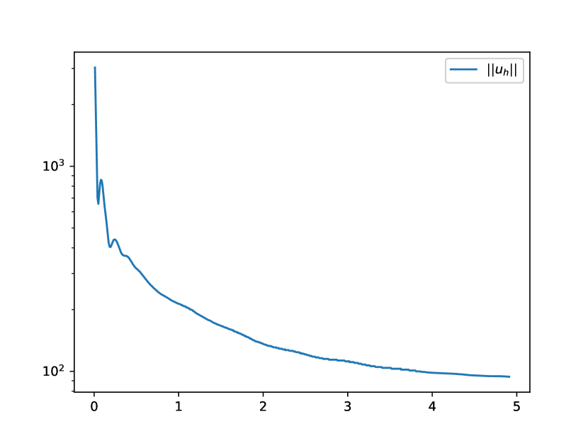
(a)

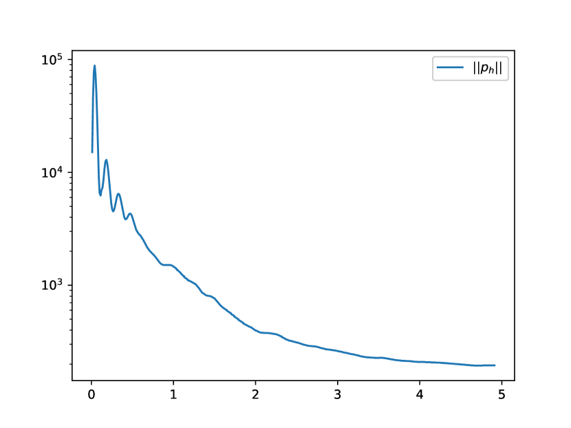
(b)

Fig. 1: Velocity and pressure norms over time $t$.

In Figure 3, we give plots of velocity magnitude at times $t=1,2,3,4$ on $\Omega$ at five cross-sections of $\Omega$.

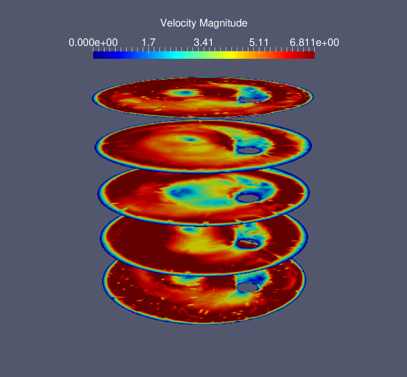
(a) $t=1$

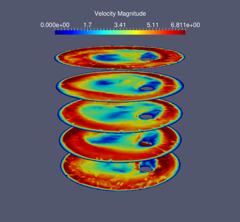
(b) $t=2$

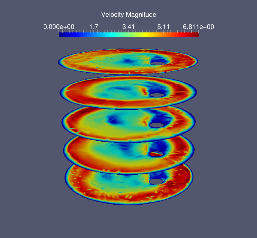
(a) $t=3$

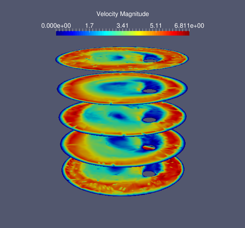
(b) $t=4$

Fig. 3: Velocity magnitude at different $t$.

5.2 Test 2: Adaptive, Variable $\varepsilon(t)$

The next test investigates self-adaptive variation of $\varepsilon_{n}$ and the resulting accuracy. We now consider a two-dimensional flow over $\Omega=~{}]0,1[^{2}$ with the exact solution

$$u(x,y;t):=\sin(t)(\sin(2\pi x)\sin^{2}(2\pi x),\sin(2\pi x)\sin^{2}(2\pi y))^{T},$$

$$p(x,y;t):=\cos(t)\cos(\pi x)\sin(\pi y)$$

and corresponding body force $f$. We let $\nu=1$, the final time $T=1$, $\varepsilon_{n}=k_{n}$, and $k_{0}=.001$. To adapt the timestep (and generate $k_{n}$), we employ a halving-and-doubling technique using $||\nabla\cdot{u_{h}}||$ as the estimator. We let the tolerance interval be $(.001,.01)$ (If $||\nabla\cdot{u_{h}}||<0.001$, $k_{n}$ and $\varepsilon_{n}$ are doubled, while if $||\nabla\cdot{u_{h}}||>0.01$, the two are halved and the step is repeated). This procedure does not control the local truncation error, only the violation of incompressibility.

The plots in Figure 4 show the velocity and pressure errors, as well as the fluctuation of $k_{n}$ and $\nabla\cdot{u}$, over time. We see that the errors of both the velocity and pressure fluctuate with changes in the timestep, as does the divergence.

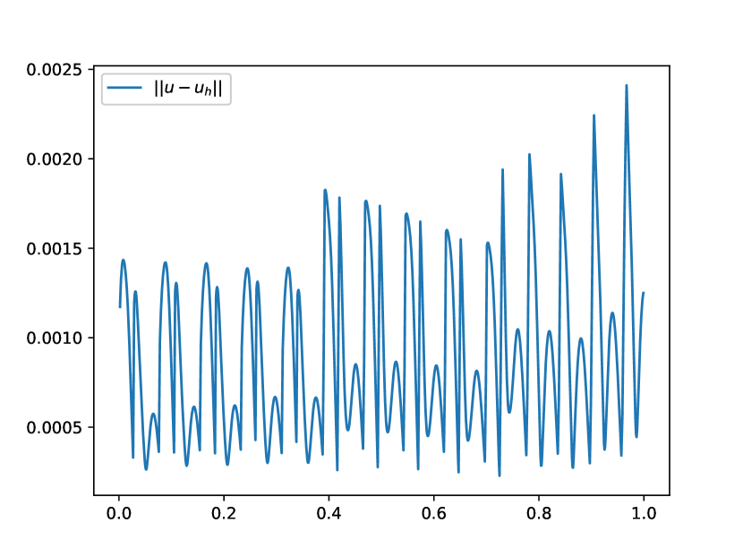
(a) Velocity error

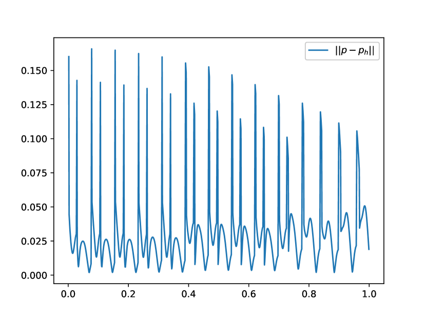
(b) Pressure error

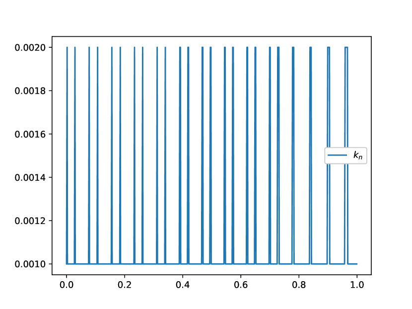
(c) Timestep evolution

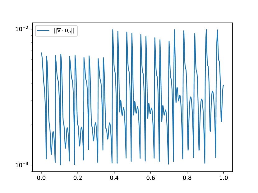
(d) Divergence evolution

Fig. 4: Accuracy and adaptability results.

Figure 4(a) shows that the velocity error is reasonable but does grow (slowly), consistent with separation of trajectories of the Navier-Stokes equations. Figure 4(d) shows $||\nabla\cdot{u_{h}}||$ is controlled. Figure 4(b) shows the pressure error actually decreases. Figure 4(c) shows that the evolution of $k_{n}$, and therefore $\varepsilon_{n}$, is not as smooth as required by condition (30). Nevertheless, the simulation produced approximations of reasonable accuracy.

6 Conclusions and future prospects

Slightly compressible fluids models provide a basis for challenging numerical simulations. Efficiency and especially time accuracy in such simulations require variable timestep and thus variable $\varepsilon=\varepsilon(t)$. Variable $\varepsilon$ is beyond existing mathematical foundations for slightly compressible models. The method and associated continuum model considered herein is modified from the standard one for variable $\varepsilon$, has been proven to be stable and converge to a weak solution of the incompressible Navier-Stokes equations as $\varepsilon(t)\rightarrow 0$, $\varepsilon_{t}(t)\rightarrow 0$ and $\varepsilon_{tt}(t)\rightarrow 0$ provided $\varepsilon_{t}(t),\varepsilon_{tt}(t)\leq C\varepsilon(t)^{1+\delta}$. The analysis of the long time stability of the standard method and model for variable $\varepsilon=\varepsilon(t)$ is an open problem with no clear entry point for its analysis (Section 2). The fluctuation condition $\varepsilon_{t}(t),\varepsilon_{tt}(t)\leq C\varepsilon(t)^{1+\delta}$ we require is too strong for practical computation. Proving convergence to an NSE weak solution under a relaxation of the condition is an important open problem. Preliminary numerical tests in Section 5 with halving and doubling (which does not satisfy the condition) suggest that the condition $\varepsilon_{t}(t),\varepsilon_{tt}(t)\leq C\varepsilon(t)^{1+\delta}$ should be improvable. Other open questions include convergence of flow quantities (e.g., vorticity, lift, drag, energy dissipation rates, $Q$-criterion values and so on) to their incompressible values as $\varepsilon(t),\varepsilon_{t}(t)\cdot\cdot\cdot\rightarrow 0$, derivation of the rates of convergence for strong solutions and extension of the analysis herein.

References

- [Al15] M. Alnæs, J. Blechta, J. Hake, A. Johansson, B. Kehlet, A. Logg, C. Richardson, J. Ring, M.E. Rognes, G.N. Wells, The FEniCS project version 1.5, Archive of Numerical Software 3 (2015), 9–23.
- [Au63] J. Aubin, Un théorème de compacité, C. R. Acad. Sci. Paris 256 (1963), 5042–5044.
- [BS15] L. C. Berselli, S. Spirito, On the construction of suitable weak solutions to the 3D Navier-Stokes equations in a bounded domain by an artificial compressibility method, arXiv:1504.07800, 2015.
- [C68] A. J. Chorin, Numerical solution of the Navier-Stokes equations, Mathematics of computation 22 (1968), 745–762.
- [C69] A. J. Chorin, On the convergence of discrete approximations to the Navier-Stokes equations, Mathematics of computation 23 (1969), 341–353.
- [RL14] T. Chaćon Rebollo and R. Lewandowski, Mathematical and numerical foundations of turbulence models and applications, Modeling and Simulation in Science, Engineering and Technology, Birkhauser/Springer, New York, 2014.
- [CHOR17] S. Charnyi, T. Heister, M. Olshanskii, and L. Rebholz, On conservation laws of Navier-Stokes Galerkin discretizations, Journal of Computational Physics, 337, 289-308, 2017.
- [DLM17] V. DeCaria, W. Layton and M. McLaughlin, A conservative, second order, unconditionally stable artificial compression method, CMAME 325 (2017), 733–747.
- [DM06] D. Donatelli and P. Marcati, A dispersive approach to the artificial compressibility approximations of the Navier-Stokes equations in 3D, J. Hyperbolic Differ. Equ. 3 (2006), 575–588.
- [DM10] D. Donatelli and P. Marcati, Leray weak solutions of the incompressible Navier Stokes system on exterior domains via the artificial compressibility method, Indiana Univ. Math. J. 59 (2010), 1831–1852.
- [DS11] D. Donatelli and S. Spirito, Weak solutions of Navier-Stokes equations constructed by artificial compressibility method are suitable, J. Hyperbolic Differ. Equ. 8 (2011), 101–113.
- [GV95] J. Ginibre and G. Velo, Generalized Strichartz inequalities for the wave equation, J. Funct. Anal. 133 (1995), 50–68.
- [GMS06] J. Guermond, P. Minev and J. Shen, An overview of projection methods for incompressible flows, Comput. Methods Appl. Mech. Engrg. 195 (2006), 6011–6045.
- [GM15] J.-L. Guermond and P. Minev, High-Order Time Stepping for the Incompressible Navier–Stokes Equations, SIAM J. Sci. Comput. 37-6 (2015), A2656-A2681 http://dx.doi.org/10.1137/140975231.
- [GM17] J.-L. Guermond and P. Minev, High-order time stepping for the Navier–Stokes equations with minimal computational complexity, JCAM 310 (2017), 92–103.
- [GM18] J.-L. Guermond and P. Minev, High-order, adaptive time stepping scheme for the incompressible Navier–Stokes equations, technical report 2018.
- [G89] M.D. Gunzburger, Finite Element Methods for Viscous Incompressible Flows - A Guide to Theory, Practices, and Algorithms, Academic Press, 1989.
- [GS00] P.M. Gresho and R.L. Sani, Incompressible flows and the finite element method, volume 2, John Wiley and Sons, Chichester, 2000.
- [JL04] H. Johnston and J.-G. Liu, Accurate, stable and efficient Navier-Stokes solvers based on an explicit treatment of the pressure term, JCP 199(2004) 221-259.
- [K86] J. Van Kan, A second order accurate pressure-correction scheme for viscous incompressible flow, SIAM J. Sci. Computing 7(1986), 870–891.
- [KT98] M. Keel and T. Tao, Endpoint Strichartz estimates, Amer. J. Math. 120 (1998), 955-980.
- [KM93] S. Klainerman and M. Macedon, Space-time estimates for null forms and the local existence theorem, Comm. Pure Appl. Math. 46 (1993), 1221–1268.
- [K02] G.M. Kobel’kov, Symmetric approximations of the Navier-Stokes equations, Sbornik: Mathematics. 193(2002), 1027-1047.
- [L84] W. Layton, An Energy Analysis of a Degenerate Hyperbolic Partial Differential Equations, Aplikace Matematiky, 29 (1984) 350-366.
- [L59] J. L. Lions, Sur l’existence de solutions des équations de Navier-Stokes, C. R. Acad. Sci. Paris 248 (1959), 2847–2849.
- [L69] J. L. Lions, Quelque méthodes de résolution des problemes aux limites non linéaires, Paris: Dunod-Gauth. Vill. (1969).
- [L96] P. L. Lions, Mathematical Topics in Fluid Mechanics: Volume 2: Compressible Models, Oxford University Press on Demand, 1996.
- [MSS93] G. Mockenhaupt, A. Seeger and C. D. Sogge, Local smoothing of Fourier integral operators and Carleson-Sjölin estimates, J. Amer. Math. Soc. 6 (1993), 65–130.
- [OA10] T. Ohwada and P. Asinari, Artificial compressibility method revisited: Asymptotic numerical method for incompressible Navier Stokes equations. J. Comp. Physics, 229:16981723, 2010.
- [O71] A. Oskolkov, On a quasi-linear parabolic system with a small parameter approximating the Navier-Stokes system, Zapiski Nauchnykh Seminarov POMI 21 (1971), 79–103.
- [P97] A. Prohl, Projection and quasi-compressibility methods for solving the incompressible Navier-Stokes equations, Springer, Berlin, 1997.
- [S92a] J. Shen, On error estimates of projection methods for the Navier-Stokes equations: First Order Schemes, SINUM 29 (1992), 57-77.
- [S96] J. Shen, On a new pseudocompressibility method for the incompressible Navier-Stokes equations, Appl. Numer. Math. 21 (1996), 71–90.
- [S98] H. F. Smith, A parametrix construction for wave equations with coefficients, Ann. Inst. Fourier (Grenoble) 48 (1998), 797–835.
- [SFR18] G. Söderlind, I. Fekete and I. Faragó, On the 0-stability of multistep methods on smooth nonuniform grids, arXiv: 1804.04553, 2018.
- [S95] C. Sogge, Lectures on Nonlinear Wave Equations, International Press, Cambridge, MA, 1995.
- [St16] E. M. Stein, Harmonic Analysis (PMS-43), Volume 43: Real-Variable Methods, Orthogonality, and Oscillatory Integrals.(PMS-43), vol. 43, Princeton University Press, 2016.
- [S77] R. S. Strichartz, Restrictions of Fourier transforms to quadratic surfaces and decay of solutions of wave equations, Duke Math. J. 44 (1977), 705–714.
- [Ta00] D. Tataru, Strichartz estimates for operators with nonsmooth coefficients and the nonlinear wave equation, Amer. J. Math. 122 (2000), 349–376.
- [Ta01] D. Tataru, Strichartz estimates for second order hyperbolic operators with nonsmooth coefficients. II, Amer. J. Math. 123 (2001), 385–423.
- [Ta02] D. Tataru, Strichartz estimates for second order hyperbolic operators with nonsmooth coefficients. III, J. Amer. Math. Soc. 15 (2002), 419–442.
- [T69I] R. Temam, Sur l’approximation de la solution des équations de Navier-Stokes par la méthode des pas fractionnaires (I), Arch. Ration. Mech. Anal. 32 (1969), 135–153.
- [T69II] R. Temam, Sur l’approximation de la solution des équations de Navier-Stokes par la méthode des pas fractionnaires (II), Arch. Ration. Mech. Anal. 33 (1969), 377–385.
- [T83] R. Temam, Navier-Stokes Equations and Nonlinear Functional Analysis, CBMS-NSF Regional Conference Series in Applied Mathematics, 41, SIAM, Philadelphia, PA (1983).
- [T01] R. Temam, Navier-Stokes equations, AMS Chelsea Publishing, Providence, RI, 2001.
- [YBC16] L. Yang, S. Badia and R. Codina, A pseudo-compressible variational multiscale solver for turbulent incompressible flows, Comp. Mechanics 58(2016) 1051-1069.
- [Z06] R.Kh. Zeytounian, Topics in hyposonic flow theory, LN in Physics, Springer, Berlin, 2006.