Non-equilibrium dynamics of isostatic spring networks

Abstract

Marginally stable systems exhibit rich critical mechanical behavior. Such isostatic assemblies can be driven out of equilibrium by internal activity, but it remains unclear how the isostatic and critical nature of such systems affects their non-equilibrium dynamics. Here, we investigate the influence of the isostatic threshold on the non-equilibrium dynamics of active diluted spring networks. In our model, heterogeneously distributed active noise sources drive the system into a non-equilibrium steady state. We quantify the non-equilibrium dynamics of nearest-neighbor network nodes by the characteristic cycling frequency $\omega$—a measure of the circulation of the associated phase space currents. The distribution of these nearest-neighbor cycling frequencies exhibits critical scaling, which we describe using a mean-field approach. Overall, our work provides a theoretical approach to elucidate the role of marginality in active disordered systems.

Isostaticity has been central in providing a unified understanding of the mechanics of soft disordered systems Liu and Nagel (1998); van Hecke (2010); Lubensky et al. (2015); Broedersz and MacKintosh (2014). A system is isostatic when its degrees of freedom are exactly balanced by its internal constraints, poising the system at the verge of mechanical stability Maxwell (1864); Jacobs and Thorpe (1996). Examples of such marginal matter include colloidal suspensions, granular packings and foams near the jamming transition Cates et al. (1998); Liu and Nagel (2010), as well as spring lattices Thorpe (1983); Wyart et al. (2008); Mao et al. (2010) and biological fiber networks Heussinger and Frey (2006); Broedersz et al. (2011); Broedersz and MacKintosh (2014). Such systems display critical behavior near the isostatic connectivity point such as universality, a nonlinear elastic response, and diverging strain fluctuations Broedersz et al. (2011); Sheinman et al. (2012); Broedersz and MacKintosh (2014); Lubensky et al. (2015); Sharma et al. (2016). Recently, a variety of non-equilibrium dynamics has been reported in active soft matter, ranging from biopolymer assemblies with molecular motors Alvarado et al. (2013); Brangwynne et al. (2008); Schaller et al. (2010); Huber et al. (2018) and vibrated polar disks Deseigne et al. (2010) to living systems such as cells, tissues and bacterial populations Angelini et al. (2011); Bi et al. (2015); Thutupalli et al. (2015); Delarue et al. (2016). Although there is evidence that such collective dynamics occurs in the vicinity of an isostatic threshold Alvarado et al. (2013); Bi et al. (2015); Tan et al. (2018); Alvarado et al. (2017), it remains unclear to what extent the critical nature of these systems affects their non-equilibrium dynamics Woodhouse et al. (2018); Wan and Goldstein (2018). More generally, a theoretical framework for the non-equilibrium stochastic dynamics of marginally stable systems is still lacking.

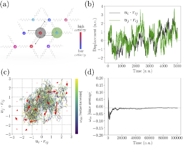
Figure 1: (a) Schematic of a driven disordered network of beads and springs: bead colors indicate local active noise amplitudes, increasing from blue to red. We consider the coupled stochastic dynamics of nearest-neighbor beads (double arrows): for all such pairs we calculate the cycling frequency $\omega_{\text{\tiny{NN}}}$. (b) The displacements of two nearest-neighbor beads projected along the associated bond directions (panel (a)) as a function of time. All quantities are plotted in natural units (see main text). (c) Phase space trajectory (colored by the instantaneous cycling frequency) and probability current (red arrows) for the data in panel (b). (d) The time-averaged cycling frequency converges to a non-zero value as $t\rightarrow\infty$.

Here we propose a simple model for an internally driven marginal elastic system: an active randomly diluted triangular network with tunable connectivity. This model allows us to systematically investigate the role that the isostatic connectivity point plays in controlling the system’s non-equilibrium fluctuations. In our model we consider a heterogeneous distribution of active sources at the nodes: activity differences drive the network out of equilibrium, thereby breaking detailed balance (Fig. 1(a)). At steady state, broken detailed balance is associated with the presence of circulating probability currents in the phase space of configurational observables Battle et al. (2016); Gnesotto et al. (2018). Consequently, the phase space trajectory of a pair of degrees of freedom circulates on average with a cycling frequency $\omega$ (Fig. 1(c)-(d)). We employ this measure to quantify broken detailed balance between pairs of directly connected nodes Weiss (2003); Gladrow et al. (2016, 2017). Interestingly, as we lower the network connectivity, we find that the distribution of cycling frequencies changes drastically near the isostatic threshold. To characterize this transition, we use the $68_{\rm th}$ percentile of this distribution as an order parameter. We support our choice by demonstrating that the $68_{\rm th}$ percentile obeys characteristic scaling laws in the form of a homogeneity relation, and we develope a mean-field theory for this scaling behavior. Taken together, our results demonstrate how isostaticity can control the non-equilibrium dynamics in disordered systems.

We start our analysis by considering an elastic network of beads connected by springs arranged on a triangular lattice in 2D. The lattice is immersed in an incompressible newtonian fluid at temperature $T$ and all springs have elastic constant $k$ and rest length $\ell_{0}$ (Fig. 1(a)). To tune network connectivity, we randomly dilute bonds with probability $1-p$, with $p\in[0,1]$, resulting in a network of average connectivity $z=6p$. The overdamped stochastic equation for the position $\mathbf{x}_{i}$ of each node reads

$$\gamma\frac{d\mathbf{x}_{i}}{dt}(t)=-\sum_{\langle i,j\rangle}k_{i,j}(\lVert\mathbf{x}_{i,j}(t)\rVert-\ell_{0})\hat{\mathbf{x}}_{i,j}(t)+a_{i}\boldsymbol{\mathbf{\eta}}_{i}(t)\,,$$ (1)

where $\gamma$ is the drag coefficient of each bead in the fluid, $k_{i,j}=k$ if the bond is present or $k_{i,j}=0$ if the bond is removed, $\mathbf{x}_{i,j}=\mathbf{x}_{i}-\mathbf{x}_{j}$, and $\hat{\mathbf{x}}_{i,j}$ is the corresponding unit vector. Note, we neglect hydrodynamic interactions between beads and use fixed boundary conditions to prevent rigid body translation and rotation.

Internal fluctuating forces acting on the beads are described as Gaussian white noise. Thus, for nodes $i$ and $j$, $\langle\eta_{ix}(t)\eta_{jy}(t^{\prime})\rangle=\delta_{ij}\,\delta_{xy}\,\delta(t-t^{\prime})$ and $\langle{\eta}_{ix}\rangle=\langle\eta_{iy}\rangle=0$. Here, the white noise amplitude includes both thermal and active fluctuations: $a_{i}=\sqrt{2\gamma k_{B}(T+|\alpha_{i}|})$. Importantly, while the amplitude of the thermal contribution is homogeneous throughout the system, the amplitude of active noise may be heterogeneous and will be described using quenched disorder. Specifically, we draw the amplitudes $\alpha_{i}$ from a normal distribution with average $\mu_{\alpha}$ and variance $\sigma_{\alpha}^{2}$, such that $\sigma_{\alpha}\ll T+\mu_{\alpha}$. This approach allows us to investigate a general scenario of marginally stable system driven out of equilibrium by internal driving. Note, when $\sigma_{\alpha}=0$, the system obeys equilibrium dynamics. In what follows we use natural units, measuring time in units of $\gamma/k$, lengths in units of $\ell_{0}$ and temperature (and activity) in units of $k\ell_{0}^{2}/k_{B}$, leaving only $a_{i}=\sqrt{2(T+|\alpha_{i}|)}$ free in Eq. (1).

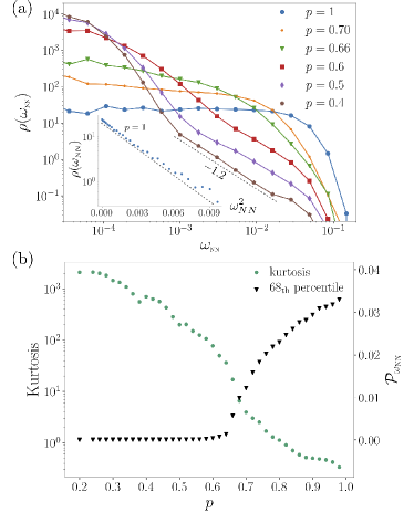
Figure 2: (a) The probability density of cycling frequencies $\rho(\omega_{\text{\tiny{NN}}})$, for various $p$. Inset shows that the distribution is approximately Gaussian when the network is barely diluted (i.e. $p\lesssim 1$). (b) The kurtosis (orange triangles) and the $68_{\rm th}$ percentile $\mathcal{P_{\omega_{\text{\tiny{NN}}}}}$ (green circles) of the cycling frequency distribution, for different values of $p$. These results are obtained by simulating a $100\times 100$ system with $\sigma_{\alpha}=10^{-5},\,T+\mu_{\alpha}=10^{-4}$.

To simulate our model we employ a Brownian Dynamics approach: this allows us, for instance, to track the displacements of two neighboring beads in the network. Two typical trajectories are shown in Fig. 1(b). Although we could, in principle, compute the probability current field (red arrows in Fig. 1(c)), a simpler but still meaningful way of quantifying the non-equilibrium dynamics of these two beads is the cycling frequency - the average number of revolutions of the trajectory around the origin in phase space per unit time. In general, the instantaneous cycling frequency is a random variable (Fig. 1(c)), but its time-averaged value, $\omega_{\text{\tiny{NN}}}$, assumes a well defined value in the long time limit (Fig. 1(d)) Weiss (2003); Gladrow et al. (2016, 2017), which is related to the entropy production rate Mura et al. (2018). Thus, by determining the cycling frequencies, we assign a simple pseudoscalar measure of non-equilibrium to each pair of connected neighboring beads in our network. The cycling frequencies for distinct bead pairs will in general not only differ because of the heterogeneous activities, but also because of the disordered network structure.

To investigate the interplay between internal driving and disorder, we determine the (symmetric) probability distribution, $\rho(\omega_{\rm NN})$, of nearest-neighbor cycling frequencies $\omega_{\rm NN}$ for different values of the dilution parameter $p$ (Fig. 2(a)). Given that the activity magnitudes are drawn from a normal distribution, it is perhaps not surprising that at $p=1$ the cycling frequencies are also normally distributed (inset Fig. 2(a)). Interestingly however, as we dilute the network down to the isostatic threshold for this system size ($p_{c}\approx 0.65$ Sup ), a pronounced peak develops around the origin. Furthermore, slowly decaying heavy tails with an apparent power-law dependence characterize the distribution for large $\omega_{\rm NN}$ (Fig. 2(a)); correspondingly, the kurtosis of the distribution increases markedly as we lower $p$ (Fig. 2(b)). These results indicate that the standard deviation is not appropriate to characterize the cycling frequency distribution. Instead, we use the 68_th percentile, $\mathcal{P_{\omega_{\text{\tiny{NN}}}}}$, of the distribution; $\mathcal{P_{\omega_{\text{\tiny{NN}}}}}$ is non-zero in the rigid (ordered) phase $p>p_{c}$, while it falls to zero continuously when $p<p_{c}$.

To provide intuition for what features determine the distribution of cycling frequencies, we first ask what sets the local value of $\omega_{\rm NN}$. It is instructive to start by considering a purely elastic network where all thermal and active fluctuations have been suppressed. Specifically, we determine the linear response of the system to three configurations of forces applied to a pair of neighboring nodes in the network: two monopoles and one dipole force, all directed along the lattice bond connecting the two beads, as in Fig. 3(a). By assessing the directed displacements of the beads for each of the three force configurations, we measure three different elastic responses. Using these responses, we map the local mechanical response in the disordered network onto an effective one-dimensional two-bead model (Fig. 3(b)) with spring constants $k_{1},k_{2},k_{12}$. These spring constants are set such that the effective system retains the same elastic response to the three force configurations as the local response in the full network.

While this procedure works well for a purely mechanical network, the mapping is in general not valid for the stochastic dynamics of the active system Mehl et al. (2012); Uhl et al. (2018). However, we can, as a first approximation, neglect the active fluctuations of all other beads in the network and insert in our two-bead model only the activities of the considered pair of nodes (Fig. 3(b)). By ascribing the same activities of the pair of nodes in the network to the nodes of the effective two-bead model, we can make a prediction for the cycling frequencies. In the limit of small activity difference, i.e. $\alpha_{1}=T+\alpha+\delta\alpha,\,\alpha_{2}=T+\alpha$ with $\delta\alpha\ll T+\alpha$, the cycling frequency for the two-bead model reads Sup

$$\omega_{\text{\tiny{2B}}}\approx k_{12}\frac{\sqrt{k_{12}(k_{1}+k_{2})+k_{1}k_{2}}}{k_{1}+2k_{12}+k_{2}}\frac{\delta\alpha}{T+\alpha}.$$ (2)

The cycling frequencies $\omega_{\text{\tiny{NN}}}$ for every pair of neighbors in the full disordered network agree well on a case by case basis with the estimates of the two-bead model $\omega_{\text{\tiny{2B}}}$ (Fig. 3(c)). However, the cycling frequencies $\omega_{\text{\tiny{2B}}}$ predicted by the two-bead model are, in absolute value, larger than the ones obtained from our network simulations. We attribute this effect to the activities of the other network nodes Sup , which are excluded in this simple model. Nonetheless, these results indicate that the local mechanical response together with the local activity difference set the scale of the local cycling frequency.

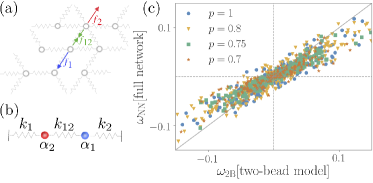
Figure 3: (a) Two monopole forces $f_{1}$ and $f_{2}$ and a dipole $f_{12}$ are applied at two neighboring network nodes. The response to the forces yields three different effective spring constants $k_{1},k_{2},k_{12}$. (b) Two-bead model with activities equal to those of the nodes in the full network. (c) Scatter plot of the cycling frequencies $\omega_{\text{\tiny{NN}}}$ calculated for each pair of neighboring nodes for full networks with varying $p$ (y-axes) and the corresponding estimate from the two-bead model $\omega_{\text{\tiny{2B}}}$ (x-axes).

Studying analytically the full system described by Eq. (1) is arduous, as nonlinearities may become increasingly more important when the system is diluted and driven out of equilibrium by large noise. However, in the limit of modest driving, the elastic contribution to the force in our model can be linearized, which results in a simplified equation of motion (in natural units)

$$\frac{d\mathbf{u}_{i}}{dt}(t)=-\sum_{\langle j\rangle}A_{ij}\mathbf{u}_{j}+a_{i}\boldsymbol{\mathbf{\eta}}_{i}(t)\,,$$ (3)

with $\mathbf{u}_{i}$ representing the displacement of node $i$ from its rest position and the elastic-matrix $A$ being defined as

$$A_{i\alpha j\beta}=\begin{cases}-k_{i,j}\hat{r}_{i,j\alpha}\hat{r}_{i,j\beta},&i\neq j\\ \sum\limits_{n\neq i}k_{in}\hat{r}_{i,n\alpha}\hat{r}_{i,n\beta},&i=j\end{cases}\,,$$ (4)

where $\hat{\mathbf{r}}_{i,j}$ is the unit vector connecting the rest positions of nodes $i$ and $j$ and greek indices denote cartesian components. For such a linear system, the steady-state covariance matrix $C_{i\alpha j\beta}=\langle{u}_{i\alpha}{u}_{j\beta}\rangle$ satisfies the Lyapunov equation Lyapunov (1950):

$$AC+CA^{T}=-2D\,,$$ (5)

with $D$ being the diffusion matrix with elements $D_{i\alpha j\beta}=\frac{1}{2}a_{i}^{2}\delta_{ij}\delta_{\alpha\beta}$. While for a fully connected network $A$ is invertible, zero-energy modes with diverging relaxation time start to appear in the system as we remove bonds from the network and approach the isostatic point $p_{c}$. Infinite relaxation times lead to divergences in the elements of the covariance matrix. To avoid these divergences, it is convenient to insert a weak $\varepsilon$-spring of elastic constant $\varepsilon\ll 1$ ($\varepsilon$ is in units of $k$) whenever a $k$-spring is removed, as sketched in Fig. 4(a)  Garboczi and Thorpe (1986); Wyart et al. (2008). In the limit $\varepsilon\to 0$ we expect to recover the dynamics of the simulated network. This dilute-and-replace procedure allows us to stabilize the zero modes in a controlled way, thereby avoiding singularities of the covariance matrix. Because of the 6-fold rotational symmetry of the lattice, we obtain the cycling frequencies by considering a specific direction, namely for $x$-displacements of nodes connected by $x$-directed bonds Mura et al. (2018):

$$\omega_{ij}=\frac{1}{2}\frac{\left(AC-CA^{T}\right)_{ixjx}}{\sqrt{C_{ixix}C_{jxjx}-C_{ixjx}C_{jxix}}}\,.$$ (6)

In the limit of modest activity: $\sigma_{\alpha}\ll(T+\mu_{\alpha})\ll 1$, the full non-linear model (Eq. (1)) is well approximated by its linearized version (Eq. (3)). As a result, we can numerically obtain the distributions of Fig. 2(a) and in particular the observable $\mathcal{P_{\omega_{\text{\tiny{NN}}}}}$. Moreover, the introduction of a soft spring constant $\varepsilon$ allows us to stabilize the rigidity of our network also below $p_{c}$. Using this approach, we find that the characteristic change in the shape of $\rho(\omega_{\text{\tiny{NN}}})$ near the critical point $p_{c}$ (see Fig. 2(b)), is reflected by a sharp but continuous decrease of $\mathcal{P_{\omega_{\text{\tiny{NN}}}}}$, as shown in Fig. 4(b) for varying $\varepsilon$.

Because the network is stabilized by the soft $\varepsilon$-springs, the jump in $\mathcal{P_{\omega_{\text{\tiny{NN}}}}}$ becomes less pronounced for larger values of $\varepsilon$. Thus, it appears as if $\varepsilon$ acts as a scaling field that takes the system away from criticality Wyart et al. (2008); Broedersz et al. (2011). To test this idea, we investigate if $\mathcal{P_{\omega_{\text{\tiny{NN}}}}}$ obeys a homogeneity relation of the form

$$\mathcal{P_{\omega_{\text{\tiny{NN}}}}}(p,\varepsilon)=|\Delta p|^{f}P_{\pm}(\varepsilon|\Delta p|^{-\phi})\,,$$ (7)

where $\Delta p=p-p_{c}$ and $P_{\pm}$ is a universal function. To this end, we rescale the data for different $\varepsilon$ and $p$ according to this relation and observe a good collapse, as shown in Fig. 4(d). Based on this analysis, we identify three distinct scaling regimes: a super-critical, $k$-dominated regime where $\mathcal{P_{\omega_{\text{\tiny{NN}}}}}\sim|\Delta p|^{f}$, a critical regime $\mathcal{P_{\omega_{\text{\tiny{NN}}}}}\sim\varepsilon^{f/\phi}$, and a sub-critical one where $\mathcal{P_{\omega_{\text{\tiny{NN}}}}}\sim\varepsilon^{1/2}|\Delta p|^{f-\phi/2}$. Empirically, we observe a reasonable collapse with the exponents $f=0.45\pm 0.05,\,\phi=1.8\pm 0.2$.

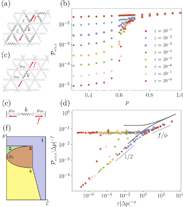
Figure 4: (a) Schematic of network with $\varepsilon$-bond replacement. (b) The $68_{\rm th}$ percentile, $\mathcal{P_{\omega_{\text{\tiny{NN}}}}}$ for different $p$ and $\varepsilon$. These results were obtained by solving Eq. (5) for a triangular lattice of size $W=40\times 40$ and $\sigma_{\alpha}=10^{-4},\,T+\mu_{\alpha}=10^{-3}$.(c) Schematic of effective medium, with all bonds replaced by effective medium springs except for the bonds where the dipole is applied. (d) Scaling of the $68_{\rm th}$ percentile $\mathcal{P_{\omega_{\text{\tiny{NN}}}}}(p,\varepsilon)=|\Delta p|^{f}P(\varepsilon|\Delta p|^{-\phi})$ around the critical point. The solid line indicates the mean-field prediction. (e) Effective two-bead model with external spring constants $\mu_{m}$. (f) Schematic phase diagram: (1) $\mathcal{P_{\omega_{\text{\tiny{EMT}}}}}\sim k$; (2) $\mathcal{P_{\omega_{\text{\tiny{EMT}}}}}\sim k^{1/2}|\Delta p|^{1/2}$; (3) $\mathcal{P_{\omega_{\text{\tiny{EMT}}}}}\sim k^{3/4}\varepsilon^{1/4}$; (4) $\mathcal{P_{\omega_{\text{\tiny{EMT}}}}}\sim k^{1/2}\varepsilon^{1/2}|\Delta p|^{-1/2}$.

To provide insight into the origin of the critical scaling of the cycling frequency distribution, we build on the two-bead model (Fig. 3) to develop a mean-field approach. In particular, we use an effective medium theory (EMT) to predict the statistical properties of the cycling frequencies in our system. Importantly, we anticipate this approach to work well in the low activity limit because of the structure of Eq. (2): fluctuations in the elastic constants of the two-bead model only appear as a second order correction to the cycling frequency Sup . Thus, a mean-field prediction of the elastic constants $k_{1}$, $k_{2}$, and $k_{12}$ of the two bead model, should lead to an accurate estimate of the cycling frequencies for the full network.

The idea underlying the EMT is to map a lattice with randomly diluted bonds onto a network with uniform bond-stiffness $\mu_{m}$ Feng et al. (1985). This is accomplished by requiring equal elastic response between the effective medium and the disordered network when applying a dipole-force between two nodes, as illustrated in Fig. 4(a)-(c). This requirement leads to the following self-consistency equation

$$\left<\frac{\mu_{m}-k}{\mu_{m}/a^{*}-\mu_{m}+k}\right>=0\,,$$ (8)

where the average $\langle\cdot\rangle$ is taken over the distribution of stiffnesses of the network bonds. In our case the distribution of bond stiffnesses is binary $P(k_{i,j}=k)=p~{},~{}~{}~{}P(k_{i,j}=\varepsilon)=1-p~{}$, and the constant $a^{*}=p_{c}=2/3$ for a triangular network Feng et al. (1985). By solving Eq. (8) for our system, we obtain the effective spring constant $\mu_{m}$ Garboczi and Thorpe (1986).

In the next step, we map the effective network onto a two-bead model, by requiring the dipole-response of the network shown in Fig. 4(c) to be equivalent to the response of the system of two beads shown in Fig. 4(e); this amounts to demanding that the two external springs both have stiffnesses $\mu_{m}$. Finally, we employ Eq. (2) in the small activity limit $\delta\alpha/(T+\alpha)\ll 1$ to obtain an analytical estimate of the cycling frequency Sup

$$\omega_{\text{\tiny{EMT}}}\approx\frac{k}{k+\mu_{m}}\sqrt{\mu_{m}(2k+\mu_{m})}\cdot\frac{\delta\alpha}{2(T+\alpha)}\,.$$ (9)

If we choose $\alpha_{1}$ and $\alpha_{2}$—the activities of the two-bead model—to be distributed as the activities of the full network, we obtain the cycling frequency distribution $\rho(\omega_{\text{\tiny{EMT}}})$, from which we numerically calculate the $68_{\rm th}$ percentile $\mathcal{P_{\omega_{\text{\tiny{EMT}}}}}$. This mean-field model successfully predicts the scaling of the $68_{\rm th}$ percentile for the original diluted network with exponents $f=1/2$, $\phi=2$  Sup , as demonstrated by the solid curve of Fig. 4(d). Note that the two-bead overestimate of the cycling frequencies already present in Fig. 3(c), is reflected here in the small but constant shift of the solid curve relative to the data in Fig. 4(d). The various phases and their boundaries predicted by this mean-field model are summarized in the phase diagram in Fig. 4(f) (see Sup ).

Our analytical approach captures the scaling of the order parameter $\mathcal{P_{\omega_{\text{\tiny{EMT}}}}}$ as well as the associated critical exponents. More than confirming our scaling ansatz Eq. (7) (solid line Fig. 4(d)), this intuitive analytic approach provides insight into how the non-equilibrium dynamics of a disordered marginal system can be understood by employing a mean-field model.

In conclusion, we have determined theoretically how the dynamics of actively driven elastic networks are governed by the vicinity to an isostatic critical point. This was accomplished by using simple experimentally accessible quantities such as the non-equilibrium cycling frequencies between pairs of nodes. These cycling frequencies are directly related to other non-equilibrium measures, such as the entropy production rate Mura et al. (2018). Our results provide an important step towards establishing a general framework to probe the dynamics of disordered non-equilibrium systems to guide experimental studies of active marginal matter in biological Alvarado et al. (2013); Bi et al. (2015); Tan et al. (2018); Wan and Goldstein (2018) and synthetic systems Narayan et al. (2007); Deseigne et al. (2010); Palacci et al. (2013).

xin 1,…,4 See pages \mathbf{x}, of BDB_Critical_Supplement_12_09_18.pdf