Role of electron inertia and electron/ion finite Larmor radius effects in low-beta, magneto-Rayleigh-Taylor instability

Abstract

The magneto-Rayleigh-Taylor (MRT) instability has been investigated in great detail in previous work using magnetohydrodynamic and kinetic models for low-beta plasmas. The work presented here extends previous studies of this instability to regimes where finite-Larmor-Radius (FLR) effects may be important. Comparisons of the MRT instability are made using a 5-moment and a 10-moment two-fluid model, the two fluids being ions and electrons. The 5-moment model includes Hall stabilization whereas the 10-moment model includes Hall and FLR stabilization. Results are presented for these two models using different electron mass to understand the role of electron inertia in the late-time nonlinear evolution of the MRT instability. For the 5-moment model, the late-time nonlinear MRT evolution does not significantly depend on the electron inertia. However, when FLR stabilization is important, the 10-moment results show that a lower ion-to-electron mass ratio (i.e. larger electron inertia) under-predicts the energy in high-wavenumber modes due to larger FLR stabilization.

I Introduction

The Rayleigh-Taylor instability (RTI) is an instability of a fluid interface appropriately oriented in the presence of an acceleration. Conventional hydrodynamic Dimonte and Schneider (2000); Dimonte et al. (2004) and magnetohydrodynamic (MHD) Chandrasekhar (1961) simulations have been performed to study the growth of this instability for regimes ranging from space and astrophysical plasmas Jun, Norman, and Stone (1995); Stone and Gardiner (2007) to fusion plasmas Atzeni, Schiavi, and Temporal (2004); Srinivasan and Tang (2013). The single-fluid MHD model does not alter the growth rate of 2-dimensional RTI when a purely out-of-plane magnetic field is present except due to large thermal conduction and diffusion mechanisms. Hence, a single-fluid ideal-MHD model only produces an altered RTI growth compared to a neutral fluid model if there is an in-plane magnetic field that can stretch, twist, and fold due to the MHD dynamo Childress and Gilbert (1995); Srinivasan and Tang (2013). The Hall-MHD model, however, can significantly alter the growth of the RTI even in the presence of a purely out-of-plane magnetic field Huba and Winske (1998). The evolution of RTI in the presence of non-ideal effects has been less studied with significant early advances made by Huba et al Huba, Lyon, and Hassam (1987); Huba (1996); Huba and Winske (1998) to illustrate the role of Hall terms and finite Larmor radius (FLR) effects. Recent work has studied the role of non-ideal effects on RTI growth for inertial confinement fusion (ICF) regimes in the presence of magnetic fields using Hall-MHD models with results compared to experiments Manuel et al. (2012); Srinivasan, Dimonte, and Tang (2012); Gao et al. (2012); Srinivasan and Tang (2013, 2014). First observations of magneto-Rayleigh-Taylor (MRT) instability evolution in the presence of magnetic and viscous effects have been made in recent experiments Adams, Moser, and Hsu (2015). Other recent work has explored the development of secondary instabilities in single-mode RTI growth using a fully kinetic code Umeda and Wada (2016) and the role of non-MHD effects in MHD scale RTI growth Goto et al. (2015); Umeda and Wada (2017). These works have explained the importance of Hall and gyro-viscous effects on RTI growth and how the presence of these additional terms introduces secondary instabilities that alter the overall evolution of the RTI.

The presence of the Hall term can increase the growth rate of RTI significantly even with a purely out-of-plane magnetic field particularly for high-wavenumber modes. On the other hand, FLR effects can have a significant stabilizing effect on RTI growth Huba (1996) with the potential to completely stabilize high-wavenumber modes. Here, the role of electron inertia and FLR effects is studied using five moment and ten moment two-fluid modelsWang et al. (2015) with comparisons of mode growth to the Hall-MHD and hybrid simulations of Ref.[Huba and Winske, 1998]. As far as the authors are aware, ten-moment two-fluid simulations of RTI have not been studied previously. Ref.[Huba and Winske, 1998] describes the regimes of RT growth when each of Hall physics and FLR physics is included and the associated stabilization. In this work, simulations are performed in 2-dimensions using purely out-of-plane magnetic fields in the low-beta regime with the five moment and ten moment models. Any in-plane magnetic field components provide stabilization of short-wavelength modes due to the MHD dynamo even in ideal-MHD. Hence, they are neglected in this work. The five moment model includes electron inertia effects with Hall physics but no FLR effects. The ten moment model includes electron inertia effects, Hall physics, and FLR effects, with a closure for the gradient of the heat-flux tensor. This work presents results showing that electron inertia alters the RTI growth rate in regimes where the FLR effects are important. This can have significant consequences for problems where an artificial ion-to-electron mass ratio is used. It is shown that the FLR stabilization of the RTI is dominated by the ion FLR effects and the ion-to-electron mass ratio alters RTI growth in regimes where FLR effects are important.

II Problem setup

The setup of interest in this work is a 2-dimensional planar domain with a density gradient on a magnetized plasma in the presence of gravity such that it is RT unstable when perturbed. An out-of-plane magnetic field is included. The inclusion of an out-of-plane magnetic field does not alter the growth of the planar RTI from the unmagnetized case when a single-fluid MHD model is used. However, the inclusion of Hall effects and FLR effects can alter the stability criteria for RTI in such a geometry Huba and Winske (1998). What is not yet well understood is the role of electron inertia and the full pressure tensor evolution in the stability and dynamics of the magnetized RTI particularly in the nonlinear phase of instability growth. This work uses a planar geometry in 2D to study these non-MHD effects in RTI growth and evolution using five- and ten-moment two-fluid models that include a complete description of the electron continuity, momentum, and energy while also including the full pressure tensor description in the ten-moment equations. Simulations are performed initializing a low beta plasma with a purely out-of-plane magnetic field.

The parameter space spans a regime where FLR effects are significant similar to the description in Ref.[Huba and Winske, 1998]. The initial conditions use an Atwood number of $0.17$, an acceleration of $0.09$, an initial plasma beta of $0.071$, an ion-to-electron temperature ratio of $0.1$ with a hyperbolic tangent density profile and an initial pressure balance. The domain size is $3\delta_{i}$ in the x-direction and $3.75\delta_{i}$ in the y-direction, with $\delta_{i}$ representing the ion skin depth. The perturbation is initially applied to the ion and electron densities to initialize modes $3$ to $32$ Srinivasan and Tang (2012). The grid resolution used for all simulations is $1500\times 1875$ so as to sufficiently resolve all initially perturbed modes consistently across the different models.

Previous single-mode RTI simulations have been performed in a similar planar geometry using an artificial ion-to-electron mass ratio of $25$, which those authors chose for computational tractability Umeda and Wada (2016, 2017). However, as shown here, an artificially high electron mass can significantly alter the growth and dynamics of RTI particularly in the late nonlinear phase of multimode RTI. For the parameter regimes chosen, FLR effects are important and FLR stabilization is expected for selected modes. Simulations are performed to isolate ion and electron FLR effects and their individual roles in the growth and dynamics of the magneto-RTI.

III Equations and numerical method

A two-fluid plasma model is used in this work and is derived by taking moments of the Boltzmann equation and treating the electrons and ions as two separate fluids. The five-moment equation system Shumlak and Loverich (2003) results by assuming an isotropic pressure with an ideal gas equation of state. This produces Euler equations for each of the electron and ion fluids with resulting equations having homogeneous, hyperbolic parts and inhomogeneous source terms. Retaining the tensor of the second moment provides the ten-moment equations Hakim (2008) which includes the full anisotropic pressure tensor with a local collisionless heat flux closure. Maxwell’s equations are used to evolve the electromagnetic terms. A finite volume scheme is used to solve the five- and ten-moment equations Hakim, Loverich, and Shumlak (2006) in the Gkeyll code Ng et al. (2015); Cagas et al. (2017); Juno et al. (2018). To allow realistic mass ratios in the models without having the electron plasma and cyclotron frequencies restrict the time-step, the hyperbolic part of the equations are evolved explicitly using a single-step finite-volume scheme while the source terms are treated with implicitly. Operator splitting is used to solve the full system. These equation systems are described below.

III.1 Five-moment two-fluid plasma model

The equations described here are the five-moment two-fluid (5M) equations that result from taking the zeroth, first, and second moments of the Vlasov equation and they are closed with an ideal gas equation of state. Isotropic pressure is assumed and collisions are neglected. The electrons and ions are each described by the Euler equations with source terms coupling the fluids and the fields. The 5M equations are given by

$$\frac{\partial\rho_{s}}{\partial t}+\nabla\cdot(\rho_{s}\mathbf{u}_{s}) =0$$ (1)

$$\frac{\partial\rho_{s}\mathbf{u}_{s}}{\partial t}+\nabla\cdot(\rho_{s}\mathbf{u}_{s}\mathbf{u}_{s}+p_{s}\mathbf{I}) =\frac{\rho_{s}q_{s}}{m_{s}}(\mathbf{E}+\mathbf{u}_{s}\times\mathbf{B})$$ (2)

$$\frac{\partial\epsilon_{s}}{\partial t}+\nabla\cdot((\epsilon_{s}+p_{s})\mathbf{u}_{s}) =\frac{\rho_{s}q_{s}}{m_{s}}\mathbf{u}_{s}\cdot\mathbf{E}$$ (3)

where subscript, $s$, denotes electron or ion species. $q$ is the charge, $m$ is the mass, $\rho$ is the mass density, $\mathbf{u}$ is the velocity, $\mathbf{E}$ is the electric field, $\mathbf{B}$ is the magnetic field, $p$ is the pressure, and $\epsilon$ is the total energy. The energy is defined as

$$\epsilon_{s}\equiv\frac{p_{s}}{\gamma-1}+\frac{1}{2}\rho_{s}u_{s}^{2}.$$ (4)

Maxwell’s equations are used to evolve the electric and magnetic fields.

$$\frac{\partial\mathbf{B}}{\partial t}+\nabla\times\mathbf{E} =0$$ (5)

$$\frac{1}{c^{2}}\frac{\partial\mathbf{E}}{\partial t}-\nabla\times\mathbf{B} =-\mu_{0}\mathbf{J}$$ (6)

$$\nabla\cdot\mathbf{E} =\frac{\varrho_{c}}{\varepsilon_{0}}$$ (7)

$$\nabla\cdot\mathbf{B} =0$$ (8)

where $\varrho_{c}$ and $\mathbf{J}$ are the charge density and the current density defined by

$$\varrho_{c} \equiv\sum_{s}\frac{q_{s}}{m_{s}}\rho_{s}$$ (9)

$$\mathbf{J} \equiv\sum_{s}\frac{q_{s}}{m_{s}}\rho_{s}\mathbf{u}_{s}.$$ (10)

To satisfy the divergence constraints of Eqs. 7 and 8, a hyperbolic form of Maxwell’s equations is evolved to include divergence correctionsMunz et al. (2000). The fluids and fields are coupled via source terms. For a plasma of $S$ species, the 5M equations consist of $5S+8$ equations.

III.2 Ten-moment two-fluid plasma model

The ten-moment two-fluid (10M) equations are obtained by retaining the anisotropic pressure tensor of the second moment of the Vlasov equation. The following higher order moments are defined,

$$\mathcal{P}_{ij} \equiv m\int v_{i}v_{j}fd\mathbf{v},$$ (11)

$$\mathcal{Q}_{ijk} \equiv m\int v_{i}v_{j}v_{k}fd\mathbf{v}.$$ (12)

which are used to obtain the set of exact moment equations Wang et al. (2015)

$$\frac{\partial n}{\partial t}+\frac{\partial}{\partial x_{j}}(nu_{j})=0,$$ (13)

$$m\frac{\partial}{\partial t}(nu_{i})+\frac{\partial\mathcal{P}_{ij}}{\partial x_{j}}=nq(E_{i}+\epsilon_{ijk}u_{j}B_{k}),$$ (14)

$$\frac{\partial\mathcal{P}_{ij}}{\partial t}+\frac{\partial\mathcal{Q}_{ijk}}{\partial x_{k}}=nqu_{[i}E_{j]}+\frac{q}{m}\epsilon_{[ikl}\mathcal{P}_{kj]}B_{l}.$$ (15)

The square brackets around indices represent the minimal sum over permutations of free indices needed to yield completely symmetric tensors. For example $u_{[i}E_{j]}=u_{i}E_{j}+u_{j}E_{i}$. Equations (13)–(15) are 10 equations (1+3+6) for 20 unknowns ($\mathcal{Q}_{ijk}$ has 10 independent components). In general any finite set of exact moment equations will always contain more unknowns than equations. Writing

$$\mathcal{Q}_{ijk} ={Q}_{ijk}+u_{[i}\mathcal{P}_{jk]}-2nmu_{i}u_{j}u_{k}\$$ (16)

to close this system of equations we need a closure approximation for the heat-flux, ${Q}_{ijk}$, defined as

$${Q}_{ijk} \equiv m\int(v_{i}-u_{i})(v_{j}-u_{j})(v_{k}-u_{k})fd\mathbf{v}.$$ (17)

Eqs. (13)–(15), closed with an approximation for the divergence of the heat-flux tensor (along with Maxwell equations), are the ten-moment two-fluid equationsHakim (2008). For a plasma of $S$ species, they consist of $10S+8$ equations.

The heat flux closure for the ten-moment two-fluid model allows inclusion of the full pressure tensor unlike the five-moment two-fluid model which assumes isotropic pressure. Hence, the ten-moment two-fluid model can capture agyrotropy of the pressure tensor. Agyrotropy is a measure of the asymmetry of the pressure tensor about a local magnetic field direction. This information is contained in the full anisotropic pressure tensor. Several scalar measures of agyrotropy have been developed. In the following, the measure $\sqrt{Q}$, suggested by SwisdakSwisdak (2016) is used

$$Q=1-\frac{4l_{2}}{(l_{1}-P_{\parallel})(l_{1}+P_{\parallel})}$$ (18)

where $l_{1}=P_{xx}+P_{yy}+P_{zz}$, $l_{2}=P_{xx}P_{yy}+P_{xx}P_{zz}+P_{yy}P_{zz}-P_{xy}^{2}-P_{xz}^{2}-P_{yz}^{2}$, and $P_{\parallel}=\hat{\mathbf{b}}\cdot\mathbf{P}\cdot\hat{\mathbf{b}}$. Comparisons have been made between the agyrotropy calculated using a ten-moment model versus a fully kinetic model for planar problems Ng et al. (2017) and for global magnetosphere problems Wang et al. (2018). It is found that ten-moment models produce lower values of agyrotropy compared to kinetic results but the values are close in magnitude and the structures are very similar. The motivation for using a ten-moment model as opposed to a kinetic model in this work is the computational effort associated with using realistic ion-to-electron mass ratios as compared to the large computational cost of performing a 2X3V (2 spatial dimensions and 3 velocity dimensions) kinetic simulation with a realistic mass ratio. This work shows how agyrotropy changes with different ion-to-electron mass ratios and consequently, how ion-to-electron mass ratio alters RTI growth in regimes where FLR effects are important.

IV Results and Analysis

IV.1 Five-moment versus ten-moment linear theory for RT growth

Simulations are performed using the five-moment and ten-moment models for the initial conditions described in Sec. II. The chosen parameter space is in a regime where the ion FLR effects dominate resulting in FLR stabilization of short-wavelength RTI. The five-moment model captures Hall effects but does not have sufficient physics in the equations to capture FLR effects. When using the ten-moment model, which incorporates Hall effects along with FLR effects, the FLR stabilization becomes dominant.

The Hall term influences RT growth based on Huba and Winske (1998)

$$\frac{\omega^{2}}{k_{y}g}=\frac{-A+\omega/\Omega_{i}}{1-A\omega/\Omega_{i}}$$ (19)

where $A$ is the Atwood number, $g$ is the acceleration, and $\Omega_{i}$ is the ion cyclotron frequency. Including FLR effects results in higher growth rates of RTI for lower-wavenumber modes as compared to the 5M model and the RT dispersion is given by Huba and Winske (1998)

$$\omega^{2}-k_{y}^{2}A\frac{cT}{eB}\omega+k_{y}g=0$$ (20)

where $T$ is the temperature, $B$ is the magnetic field, $e$ is the elementary charge, and $c$ is the light speed. The FLR effects in the regime described here completely stabilizes modes higher than approximately 22 in the linear regime.

While the linear growth of Hall and FLR physics and the associated stabilization has been studied previously, the effect of these terms on nonlinear instability evolution remains to be understood. Of particular interest is the wavenumber spectrum that persists in the nonlinear phase of the RT growth and the dependence of the nonlinear behavior on the ion-to-electron mass ratio.

IV.2 Role of electron inertia in the five-moment model

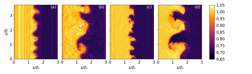
Figure 1: Ion densities after 10/$\omega_{ci0}$ (a) and 35/$\omega_{ci0}$ (b) for ion-to-electron mass ratios $M=25$ and the corresponding densities at 10/$\omega_{ci0}$ (c) and 35/$\omega_{ci0}$ (d) for $M=1836$ using the 5M model. Note the similarity in the nonlinear RT growth of the artificial mass ratio using higher electron inertia compared to the realistic mass ratio case.

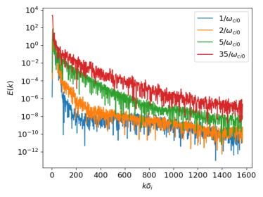
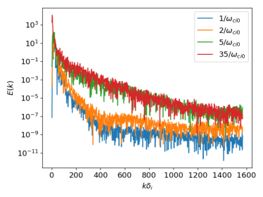
Figure 2: Power spectral density as a function of wavenumber for ion-to-electron mass ratios $M=25$ (left) and $M=1836$ (right) using the using the 5M model. Solutions are shown for several different times during the evolution. The ion density is integrated in the $x$-direction to obtain the spectrum in the $y$-direction. Note that the late-time spectra of the two mass ratios are similar.

Figure 1 presents ion density at two separate times during the evolution for multi-mode simulations with the 5M model where modes $3$ to $32$ are initialized for two ion-to-electron mass ratios of $25$ and $1836$. The perturbation is of form described in Refs.[Srinivasan, Dimonte, and Tang, 2012; Srinivasan and Tang, 2012]. The subplots (a) and (b) of Fig. 1 present the early-time and late-time evolution of the ion density for a mass ratio of $25$ and subplots (c) and (d) present early- and late-time evolution for a mass ratio of $1836$. Both ion-to-electron mass ratio simulations have higher-wavenumber modes growing early-in-time as seen in Fig. 1(a) and 1(c) (after $10/\omega_{ci0}$) compared to late-in-time in Fig. 1(b) and 1(d) (after $35/\omega_{ci0}$). The higher ion-to-electron mass ratio of $1836$ has slightly higher-wavenumber modes and larger amplitudes compared to a mass ratio of $25$, but the dominant growing modes are similar in both cases. This is further highlighted in the wavenumber spectrum for several different times shown in Fig. 2 for each of the two mass ratios presented. Note that the late-time power spectral densities (at $35/\omega_{ci0}$) do not substantially differ between the two mass ratios. While the dominant modes that remain in the solution in the nonlinear phase of instability growth are long-wavelength modes from the qualitative results of Fig. 1, the energy across all modes is approximately similar for the two mass ratios. In this regime with magnetized ions (low plasma beta), any stabilization of higher wavenumber modes is due to the Hall term and the dominant growing modes are of lower wavenumber Huba and Winske (1998) as the 5M model does not include FLR effects.

IV.3 Role of electron inertia in the ten-moment model

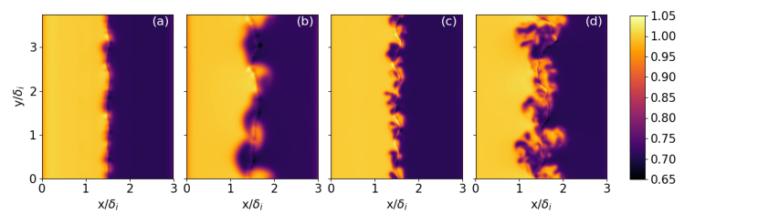
Figure 3: Ion densities after 10/$\omega_{ci0}$ (a) and 35/$\omega_{ci0}$ (b) for ion-to-electron mass ratios $M=25$ and the corresponding densities at 10/$\omega_{ci0}$ (c) and 35/$\omega_{ci0}$ (d) for $M=1836$ using the 10M model. Note the higher wavenumber modes present in the nonlinear RT growth of the realistic (higher) mass ratio case compared with the artificial (lower) mass ratio case.

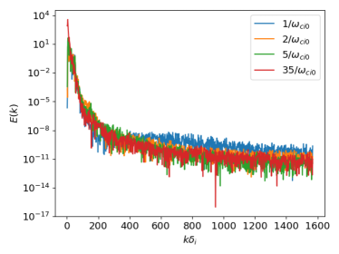
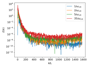
Figure 4: Power spectral density as a function of wavenumber for ion-to-electron mass ratios $M=25$ (left) and $M=1836$ (right) using the using the 10M model. Solutions are shown for several different times during the evolution. The ion density is integrated in the $x$-direction to obtain the spectrum in the $y$-direction. Note that the energy in all modes late-in-time, including higher-wavenumber modes, is higher for simulations that use a realistic mass ratio compared to a mass ratio of $25$.

For the 10M model, the electron inertia has a significant effect on RTI evolution, particularly in the late, nonlinear phase of the instability. The RTI simulations presented in Refs.[Huba, 1996; Huba and Winske, 1998] use hybrid models to incorporate FLR effects with the ions evolved kinetically and a massless electron fluid. This recovers the correct asymptotic physics in the limit of realistic ion-to-electron mass ratio. However, recent kinetic simulations of RTI Umeda and Wada (2016, 2017) use an ion-to-electron mass ratio of $25$ which could produce inaccurate nonlinear RTI evolution. The kinetic effects in these results, for example through the role of FLR effects in the RTI evolution, could significantly over-predict the stabilized modes and the nonlinear dynamics with an artificial ion-to-electron mass ratio. Figure 3 presents ion density using the 10M model for the same multimode simulation presented in Sec. IV.2 for early- and late-time evolution using the same ion-to-electron mass ratios of $25$ and $1836$.

Note that there are significant differences between the two mass ratios with the 10M model both early-in-time and late-in-time. The realistic mass ratio evolves to a greater bubble/spike propagation (amplitude) compared to the solution that uses a mass ratio of $25$. Additionally, the qualitative results of Fig. 3 clearly show that higher wavenumbers are dominant when using the realistic mass ratio. This is further noted from the power spectral density as a function of wavenumber in the $y$-direction plotted for several different times in Fig. 4. The ion density is used to create this plot and the density is integrated in the $x$-direction to obtain a domain averaged quantity describing the spectrum in the $y$-direction. A closer look at the power spectral density after $35/\omega_{ci0}$ shows that the realistic mass ratio 10M results have greater energies for high-wavenumber modes compared to results using the 10M model with a mass ratio of $25$. In fact, even as early as $5/\omega_{ci0}$, the power spectral density differs substantially for the two mass ratio results, particularly for high-wavenumber modes. A mass ratio of $25$ over-predicts the stabilization by damping out high-wavenumber modes late-in-time compared to a mass ratio of $1836$. This has implications for RT turbulence studies, when FLR effects and kinetic effects become important, as artificially higher electron mass may not capture high-wavenumber spectra accurately.

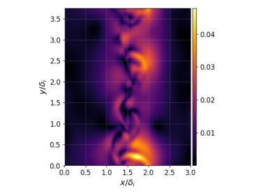
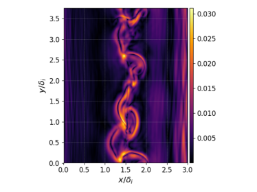
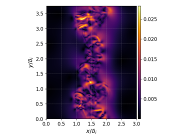
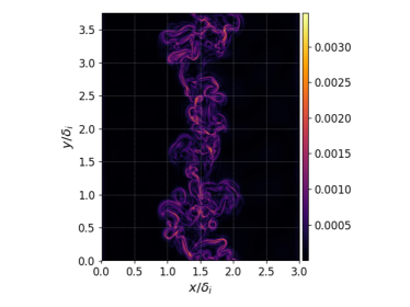
Figure 5: Ion (left) and electron (right) agyrotropy after 35/$\omega_{ci0}$ for ion-to-electron mass ratios $M=25$ (top) and $M=1836$ (bottom) using the 10M model. Note that the ion agyrotropy is approximately a factor of two lower and the electron agyrotropy is an order of magnitude lower when using a mass ratio of $1836$ compared to a mass ratio of $25$.

To address the source of differences between the 10M solutions using different mass ratios, it is illuminating to look at the ion and electron agyrotropy for these results. Figure 5 presents the agyrotropy described by Eq. 18 for the 10M simulations presented in Fig. 3 for $35/\omega_{ci0}$ using different ion-to-electron mass ratios. Note that there is a clear and significant difference in the agyrotropy when using different mass ratios. The top left plot, which presents ion agyrotropy for a mass ratio of $25$ is approximately a factor of two larger in terms of magnitude of agyrotropy compared to the bottom left plot which presents ion agyrotropy for a mass ratio of $1836$. This implies that ion FLR effects are stronger when using a lower mass ratio, and consequently the FLR stabilization is greater. Similarly, the top right plot, which presents electron agyrotropy for a mass ratio of $25$ is larger, by an order of magnitude, than the bottom right plot which presents electron agyrotropy for a mass ratio of $1836$. This indicates that the electron FLR effects are over-predicted when using an artificially small ion-to-electron mass ratio. Despite the electron agyrotropy having larger differences for the different mass ratios compared to the ion agyrotropy, “hybrid” simulations performed using 5M electrons and 10M ions reveal that the electron FLR effects do not affect the nonlinear RT dynamics and it is the ion FLR effects that dominate in the FLR stabilization noted in these simulations.

IV.4 Comparison of 5M and 10M results

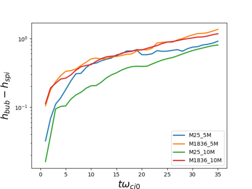
Figure 6: Bubble/spike propagation for each of the 5M and 10M models each using mass ratios of $25$ and $1836$.

The bubble/spike propagation is plotted in Fig. 6 for the 5M and 10M models each using ion-to-electron mass ratios of $25$ and $1836$. Note that, while the propagation for the different mass ratios for the 5M model converges around $15-20/\omega_{ci0}$, it begins to diverge again as the simulation evolves later in time. This may be due to an increased amount of secondary Kelvin-Helmholtz instability in the lower mass ratio simulations compared to realistic mass ratio simulations as observed from Fig. 1. The 10M model however, has significant differences in the bubble/spike propagation for all times. In addition to the lower ion-to-electron mass ratio damping higher-wavenumber modes late in time for the 10M model, the lower mass ratio 10M results also have slower bubble/spike propagation throughout compared to the realistic mass ratio results.

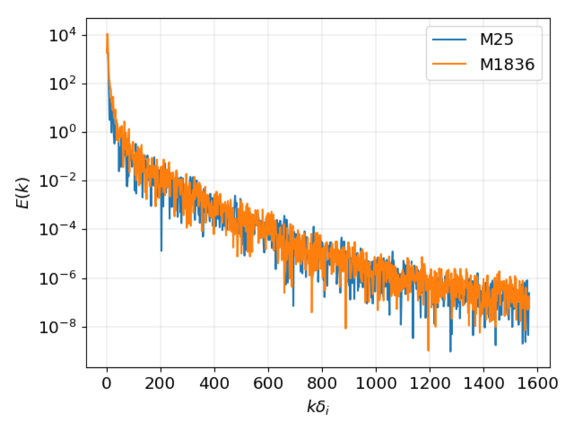
Figure 7: Power spectral density for the 5M model corresponding to a time of 35/$\omega_{cio}$ from Fig. 2 for both mass ratios of $25$ and $1836$. Note that the two ion-to-electron mass ratio simulations produce very similar power spectra.

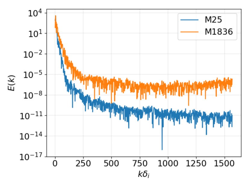
Figure 8: Power spectral density for the 10M model corresponding to a time of 35/$\omega_{cio}$ from Fig. 4 for both mass ratios of $25$ and $1836$. Note that the lower ion-to-electron mass ratio simulations have consistently lower power spectral density compared to the higher mass ratio.

Figure 7 plots the 5M model power spectral density as a function of wavenumber ($k_{y}$) at a time of $35/\omega_{ci0}$ (from Fig. 2) for each of the two mass ratios. Similarly, Fig. 8 plots the 10M model power spectral density as a function of wavenumber ($k_{y}$) at the same time (from Fig. 4) for each of the two mass ratios. To reiterate, the 5M model (Fig. 7) produces very similar power spectral densities for late-time RT for the different mass ratios. However, for the 10M model (Fig. 8), the artificially high electron mass (lower ion-to-electron mass ratio) underpredicts the power spectral density by a substantial amount (3-5 orders of magnitude) for all wavenumbers present in the spectrum and therefore over-predicts the FLR stabilization. Lastly, the significant differences in RTI evolution between the 5M and 10M results for both mass ratios are due to the absence of FLR effects in the 5M model.

V Summary

This work studies the role of ion/electron FLR effects and the role of electron inertia in the nonlinear phase of the magneto-RTI. A five-moment two-fluid model, that captures Hall effects but does not include FLR effects, is compared to a ten-moment two-fluid model which contains Hall and FLR effects for different ion-to-electron mass ratios. The simulations are performed in a regime where FLR effects are considered to be important.

The results presented here show that early-time RTI growth has slower bubble/spike propagation for a lower ion-to-electron mass ratio compared to a realistic mass ratio for both the five- and ten-moment models. Late-in-time, well into the nonlinear phase of the instability, the five-moment results with different mass ratios converge to similar bubble/spike propagation and similar dominant wavenumber spectra. However, the late-time nonlinear dynamics of the ten-moment model exhibit significant differences for the different ion-to-electron mass ratios. For a lower ion-to-electron mass ratio (i.e. with artificially large electron inertia) the bubble/spike propagation is slower than for a realistic mass ratio. Furthermore, the lower mass ratio ten-moment results damp the higher-wavenumber modes that are present in the realistic mass ratio results. Exploring the ion and electron agyrotropy shows that the lower mass ratio over-predicts both ion and electron FLR effects compared to the realistic mass ratio results which is responsible for the differences observed in the ten-moment model. However, it is the ion FLR effects that affect the FLR stabilization of high-wavenumber RT in these results for the different mass ratios.

Previous workNg et al. (2017) has compared the agyrotropy between a ten-moment model and a fully kinetic model to find that ten-moment models produce lower values of agyrotropy compared to kinetic results but the values are close in magnitude. This implies that the ten-moment results presented here are valid for understanding implications when FLR effects are important. The ten-moment model is used here for reasons of computational efficiency as compared to a well-resolved 2X3V (2 spatial dimensions and 3 velocity dimensions) fully kinetic model that would otherwise be necessary for such a study. The results presented here highlight the role of electron inertia in RTI evolution, particularly in the nonlinear phase of the instability, and have implications for problems where FLR and other kinetic effects may be important.

VI Reference

References

- Dimonte and Schneider (2000) G. Dimonte and M. Schneider, Physics of Fluids 12, 304 (2000).
- Dimonte et al. (2004) G. Dimonte, D. Youngs, A. Dimits, S. Weber, M. Marinak, S. Wunsch, C. Garasi, A. Robinson, M. Andrews, P. Ramaprabhu, et al., Physics of Fluids 16, 1668 (2004).
- Chandrasekhar (1961) S. Chandrasekhar, Hydrodynamic and hydromagnetic stability (Oxford University Press, Inc., 1961).
- Jun, Norman, and Stone (1995) B. Jun, M. Norman, and J. Stone, The Astrophysical Journal 453, 332 (1995).
- Stone and Gardiner (2007) J. M. Stone and T. Gardiner, Physics of Fluids 19, 094104 (2007).
- Atzeni, Schiavi, and Temporal (2004) S. Atzeni, A. Schiavi, and M. Temporal, Plasma Physics and Controlled Fusion 46, B111 (2004).
- Srinivasan and Tang (2013) B. Srinivasan and X.-Z. Tang, Physics of Plasmas 20, 056307 (2013).
- Childress and Gilbert (1995) S. Childress and A. Gilbert, Stretch, twist, fold: the fast dynamo (Springer, 1995).
- Huba and Winske (1998) J. D. Huba and D. Winske, Physics of Plasmas 5, 2305 (1998).
- Huba, Lyon, and Hassam (1987) J. D. Huba, J. G. Lyon, and A. B. Hassam, Physical Review letters 59, 2971 (1987).
- Huba (1996) J. Huba, Physics of Plasmas 3, 2523 (1996).
- Manuel et al. (2012) M.-E. Manuel, C. Li, F. Séguin, J. Frenje, D. Casey, R. Petrasso, S. Hu, R. Betti, J. Hager, D. Meyerhofer, et al., Physical review letters 108, 255006 (2012).
- Srinivasan, Dimonte, and Tang (2012) B. Srinivasan, G. Dimonte, and X.-Z. Tang, Physical Review Letters 108, 165002 (2012).
- Gao et al. (2012) L. Gao, P. Nilson, I. Igumenschev, S. Hu, J. Davies, C. Stoeckl, M. Haines, D. Froula, R. Betti, and D. Meyerhofer, Physical review letters 109, 115001 (2012).
- Srinivasan and Tang (2014) B. Srinivasan and X.-Z. Tang, EPL (Europhysics Letters) 107, 65001 (2014).
- Adams, Moser, and Hsu (2015) C. S. Adams, A. L. Moser, and S. C. Hsu, Physical Review E 92, 051101 (2015).
- Umeda and Wada (2016) T. Umeda and Y. Wada, Physics of Plasmas 23, 112117 (2016).
- Goto et al. (2015) R. Goto, H. Miura, A. Ito, M. Sato, and T. Hatori, Physics of Plasmas 22, 032115 (2015).
- Umeda and Wada (2017) T. Umeda and Y. Wada, Physics of Plasmas (2017).
- Wang et al. (2015) L. Wang, A. H. Hakim, A. Bhattacharjee, and K. Germaschewski, Physics of Plasmas 22, 012108 (2015).
- Srinivasan and Tang (2012) B. Srinivasan and X.-Z. Tang, Physics of Plasmas 19, 082703 (2012).
- Shumlak and Loverich (2003) U. Shumlak and J. Loverich, Journal of Computational Physics 187, 620 (2003).
- Hakim (2008) A. Hakim, Journal of Fusion Energy 27, 36 (2008).
- Hakim, Loverich, and Shumlak (2006) A. Hakim, J. Loverich, and U. Shumlak, Journal of Computational Physics 219, 418 (2006).
- Ng et al. (2015) J. Ng, Y.-M. Huang, A. Hakim, A. Bhattacharjee, A. Stanier, W. Daughton, L. Wang, and K. Germaschewski, Physics of Plasmas 22, 112104 (2015).
- Cagas et al. (2017) P. Cagas, A. Hakim, J. Juno, and B. Srinivasan, Physics of Plasmas 24, 022118 (2017).
- Juno et al. (2018) J. Juno, A. Hakim, J. TenBarge, E. Shi, and W. Dorland, Journal of Computational Physics 353, 110 (2018).
- Munz et al. (2000) C.-D. Munz, P. Omnes, R. Schneider, E. Sonnendrcker, and U. Voß, Journal of Computational Physics 161, 484 (2000).
- Swisdak (2016) M. Swisdak, Geophysical Research Letters 43, 43 (2016).
- Ng et al. (2017) J. Ng, A. Hakim, A. Bhattacharjee, A. Stanier, and W. Daughton, Physics of Plasmas 24, 082112 (2017).
- Wang et al. (2018) L. Wang, K. Germaschewski, A. Hakim, C. Dong, J. Raeder, and A. Bhattacharjee, Journal of Geophysical Research: Space Physics 41, 8688 (2018).