Probing the environment of high-z quasars
using the proximity effect in projected quasar pairs

Abstract

We have used spectra of 181 projected quasar pairs at separations $\leq 1.5$ arcmin from the Sloan Digital Sky-Survey Data Release 12 in the redshift range of 2.5 to 3.5 to probe the proximity regions of the foreground quasars. We study the proximity effect both in the longitudinal as well as in the transverse directions, by carrying out a comparison of the Ly$\alpha$ absorption lines originating from the vicinity of quasars to those originating from the general inter-galactic medium at the same redshift. We found an enhancement in the transmitted flux within 4 Mpc to the quasar in the longitudinal direction. However, the trend is found to be reversed in the transverse direction. In the longitudinal direction, we derived an excess overdensity profile showing an excess up to $r\leq 5$ Mpc after correcting for the quasar’s ionization, taking into account the effect of low spectral resolution. This excess overdensity profile matches with the average overdensity profile in the transverse direction without applying any correction for the effect of the quasar’s ionization. Among various possible interpretations, we found that the anisotropic obscuration of the quasar’s ionization seems to be the most probable explanation. This is also supported by the fact that all of our foreground quasars happen to be Type-I AGNs. Finally, we constrain the average quasar’s illumination along the transverse direction as compared to that along the longitudinal direction to be $\leq$27% (3$\sigma$ confidence level).

1. Introduction

The redshifted H i Ly$\alpha$ absorption lines seen in the spectra of distant quasars (commonly known as Ly$\alpha$ forest), are powerful probes of the physical conditions in the inter-galactic medium (IGM, Gunn & Peterson, 1965; Sargent, 1980; Rauch, 1998; Davé et al., 2010; Pieri et al., 2010) and the parameters of the background cosmology (Cocke & Tifft, 1989; Weinberg et al., 1997; Croft et al., 1998; Seljak et al., 2003; Tytler et al., 2004; Fechner & Reimers, 2007; Busca et al., 2013; Delubac et al., 2015). It is believed that most of the Ly$\alpha$ lines with column density, $N_{\rm HI}\leq 10^{14}$ cm^-2, originate from quasi-linear density fluctuations in which the hydrogen gas is in ionization equilibrium with the meta-galactic UV background (UVB) radiation produced by star-forming galaxies and quasars (Bergeron & Ikeuchi, 1990; Madau & Pozzetti, 2000; Meiksin & White, 2003; Bolton et al., 2006; Hopwood et al., 2010; Haardt & Madau, 2012; Khaire & Srianand, 2015a, b). As non-linear effects are sub-dominant, properties of the gas responsible for the Ly$\alpha$ forest can be well described using few basic ingredients such as quasi-linear theory for the growth of baryonic structure, ionization equilibrium with UVB radiation field, and the effective equation of state of the gas (Bi, 1993; Muecket et al., 1996; Bi & Davidsen, 1997; Hui et al., 1997a; Weinberg et al., 1999; Schaye, 2001a, b; Rollinde et al., 2001; Viel et al., 2002; Kim et al., 2002; Lehner et al., 2007). This basic idea is also confirmed by many hydrodynamical simulations (Cen et al., 1994; Hernquist et al., 1996; Wadsley & Bond, 1997; Zhang et al., 1997; Theuns et al., 1998; Machacek et al., 2000; Efstathiou et al., 2000; Choudhury et al., 2001a, b; Regan et al., 2007; White et al., 2010; Ozbek et al., 2016; Sorini et al., 2016; Bolton et al., 2017). Therefore, the Ly$\alpha$ forest has been extensively used to derive many cosmological properties such as matter power spectrum, baryon density in the universe, temperature and ambient radiation field (Hui & Rutledge, 1999; Nusser & Haehnelt, 1999; Pichon et al., 2001; Croft et al., 2002; McDonald et al., 2001; Viel & Haehnelt, 2006; Borde et al., 2014; Gaikwad et al., 2018) by comparing properties of simulated and observed data. Under the photoionization equilibrium, the optical depth ($\tau$) of the Ly$\alpha$ absorption in the IGM is related to the overdensity of the gas, $\Delta\equiv\rho/\langle\rho\rangle$ where, $\langle\rho\rangle$ being the mean IGM density, (e.g., see Rollinde et al., 2005, and references therein) as,

$$\tau~{}\propto~{}\Delta^{2}[T(\Delta)]^{-0.7}/\Gamma_{\textsc{Hi}}\propto\Delta^{2-0.7(\gamma-1)}/\Gamma_{\textsc{Hi}}\,.$$ (1)

Here, $\Gamma_{\textsc{Hi}}$ is the hydrogen photoionization rate, $T(\Delta)$ is the temperature of the gas at overdensity $\Delta$, given by the temperature-density relation, $T=T_{0}\Delta^{\gamma-1}$, with an exponent $\gamma$ and $T_{0}$ being the temperature at mean IGM density (i.e., $\Delta\sim$1).

Observationally, an independent way of estimating H i photoionization rate ($\Gamma_{\textsc{Hi}}$) is by the analysis of the Ly$\alpha$ absorption sufficiently close to the quasar. In this case, the UV-field is dominated by the radiation originating from the quasars which lead to a deficit of detectable Ly$\alpha$ absorption lines. As a result, contrary to the expectation that the amount of Ly$\alpha$ absorption should be an increasing function of redshift, a reversal of trend is seen for absorption redshifts close to the emission redshift of the quasar. This effect is commonly known as inverse or the proximity effect (e.g., Carswell et al., 1982; Murdoch et al., 1986; Tytler, 1987; Bajtlik et al., 1988; Kulkarni & Fall, 1993; Bechtold, 1994; Srianand & Khare, 1996; Cooke et al., 1997; Liske & Williger, 2001; Worseck & Wisotzki, 2006; Faucher-Giguère et al., 2008a; Wild et al., 2008; Prochaska et al., 2013; Khrykin et al., 2016). The strength of this effect depends on the ratio of the ionization rates contributed by the quasar and the UVB radiation. Hence, based on the extent of the proximity region along with the fact that the H i photoionization rate due to quasar radiation can be determined directly from its observed luminosity, one can infer the value of $\Gamma_{\textsc{Hi}}$ of the UVB. This method of using the line of sight proximity effect (i.e., longitudinal proximity effect) was pioneered by Bajtlik et al. (1988). Subsequent studies have yielded a wide variety of $\Gamma_{\textsc{Hi}}$ estimates varying from 1.5 to 9 in units of $10^{-12}$ s^-1 at $z=3$ (Lu et al., 1991; Kulkarni & Fall, 1993; Cristiani et al., 1995; Giallongo et al., 1996; Cooke et al., 1997; Scott et al., 2000; Liske & Williger, 2001; Dall’Aglio et al., 2008b; Calverley et al., 2011; Partl et al., 2011; Syphers & Shull, 2013).

Most of the previous measurements of $\Gamma_{\textsc{Hi}}$ using the proximity effect have assumed that the distribution of absorbing gas close to the quasar is same as that in the general IGM. This assumption may not be valid in a scenario where galaxies as well as IGM tends to cluster around the quasars (Bahcall et al., 1969; Hartwick & Schade, 1990; Bahcall & Chokshi, 1991; Fisher et al., 1996; Srianand & Khare, 1996; Fukugita et al., 2004; Croom et al., 2005; Rollinde et al., 2005; Adams et al., 2015; Eftekharzadeh et al., 2017). As a result, previous measurements might have underestimated the magnitude of the proximity effect, or equivalently, overestimated the $\Gamma_{\textsc{Hi}}$ (see also, Loeb & Eisenstein, 1995; Faucher-Giguère et al., 2008a). According to the hierarchical models of the galaxy formation, the super-massive black holes that are thought to power quasars reside in massive halos (Miralda-Escudé et al., 1996; Wyithe & Padmanabhan, 2006; Shen et al., 2007; Kim & Croft, 2008; White et al., 2012; Font-Ribera et al., 2013; Rodríguez-Torres et al., 2017), which are strongly biased towards high-density regions, especially at the higher redshifts. Therefore, it is expected that the gas in the neighborhood of the quasars must have a higher density than the gas in the general IGM at the same epoch (i.e., at same redshift).

While most such studies using Ly$\alpha$ forest were done in the longitudinal direction, the environment of a quasar can also be probed in the transverse direction using quasar pairs, commonly known as transverse proximity effect (Adelberger, 2004; Schirber et al., 2004; Rollinde et al., 2005; Worseck et al., 2007; Gonçalves et al., 2008; Gallerani, 2011; Hennawi & Prochaska, 2013; Schmidt et al., 2018). The main principle here is to use Ly$\alpha$ absorption lines detected along the sight-line of a background quasar, near the redshift of the foreground quasar, to probe the ionization effect due to a foreground quasar in the transverse direction. The absorption seen in the spectrum of the background quasar at the redshift of the foreground quasar will be influenced by the excess radiation and overdense environment in which the foreground quasar resides (e.g., see Hennawi et al., 2006; Hennawi & Prochaska, 2007; Prochaska & Hennawi, 2009; Hennawi & Prochaska, 2013; Prochaska et al., 2014; Lau et al., 2016, 2018). Many recent studies have also found a significantly more absorption close to the quasars than what is expected in the IGM and concluded that the quasars reside in regions having gas density greater than the typical gas density of the IGM (Croft, 2004; Schirber et al., 2004; Rollinde et al., 2005; Guimarães et al., 2007; Kirkman & Tytler, 2008; Finley et al., 2014; Adams et al., 2015). Recently, Prochaska et al. (2013) used a sample of 650 projected quasar pairs to study the transverse proximity effect of luminous quasars (at $z\sim 2$) at proper separations ranging from 30 kpc to 1 Mpc. Based on anisotropic absorption (also see, Prochaska et al., 2014; Lau et al., 2016, 2018) found in their analysis around quasars they concluded that the gas in the transverse direction is likely to be less illuminated by ionizing radiation compared to that along our line-of-sight to the quasars (see also, Bowen et al., 2006; Farina et al., 2013).

Another aspect one has to consider while studying the transverse proximity effect is the effect of a finite lifetime or an episodic quasar phase. Here, the extra light travel time in the perpendicular direction between the two quasar sightlines (i.e., $r_{\perp}$/c) may lead to a situation where the effect of excess radiation may be weaker or absent along line-of-sight of the background quasar sightline in the perpendicular direction from the foreground quasar when we see it in its initial stages of the active phase. Given the important implications of such studies, it is imperative to use a sample of projected quasar pairs (henceforth quasar pairs) at smaller angular separation ($<$ 1.5 arcmin), to probe the quasars environment even at kpc scales, where both the ionization effect, as well as the overdensity effect, might be appreciable. However, to lift the degeneracy due to the ionization and/or the overdensity on the observed optical depth, the measurement of UVB radiation using an independent method will be needed. For this purpose, we use the recent estimate of UVB radiation based on the updated comoving specific galaxy and quasar emissivity at different frequencies (from UV to FIR) and redshifts (Khaire & Srianand, 2015a; Khaire & Srianand, 2019). Particularly, it will help to infer any difference in the optical depth between the longitudinal and the transverse direction, to confirm or refute the validity of the assumed isotropic quasar emission and constraint the excess overdensity.

On the other hand, the advent of large quasar surveys such as Sloan Digital Sky-Survey Data Release 12 (SDSS DR12, e.g., see Pâris et al., 2017) has enabled us to gather a large sample of quasar pairs with a small separation of less than 1.5-arcmin. As a result, we can utilize these low/moderate resolution spectra of this large set of quasar pairs to probe the quasar environment and/or anisotropic emission from the quasars. In particular, it is now possible to carry out analysis using a control sample of Ly$\alpha$ absorption at the same epoch having a spectrum with a similar signal to noise and spectral resolution to that of the quasar pairs, which forms the main motivation of this work.

The paper is organized as follows. In Sect. 2 we describe our sample and selection criteria used to make the sample for the study of both the longitudinal and the transverse proximity effect along with the details of our control sample. In Sect. 3, we present pixel optical depth analysis and results along with detailed discussions on the validation of appropriate ionization corrections for the pixel optical depth from low/moderate resolution SDSS spectra using simulated spectra. The discussions are presented in Sect. 4. Finally, the summary and conclusions are given in Sect. 5. Throughout, we have used a flat background cosmology with $\Omega_{m}$ = 0.286, $\Omega_{\lambda}$ = 0.714, and $H_{o}$ = 69.6 km s^-1Mpc ^-1 (Bennett et al., 2014). All the distances mentioned in our paper are proper distances unless noted otherwise.

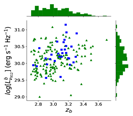
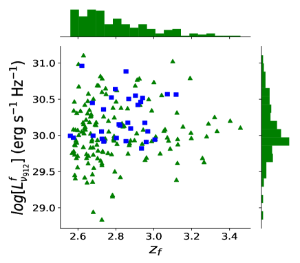
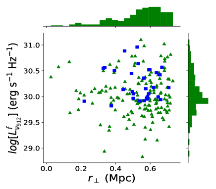
Figure 1.— Some properties of the quasars in our sample. Top: Luminosity at 912 Å (log[$L_{\nu_{912}}$] in units of erg s^-1 Hz^-1) of background quasars (listed in Table 1) versus $z_{b}$. Middle: Same as top but for the foreground quasars. Bottom: $L_{\nu_{912}}$ of the foreground quasars versus the perpendicular distance between the foreground and the background quasars at $z_{f}$. The top and right side histograms show the distribution of parameters labeled at abscissa and ordinate respectively. The blue squares are the quasars found in common with the sample of Prochaska et al. (2013).

Table 1 Basic properties of 181 quasar pairs in our sample.

SN.	Background quasar	$z_{b}$	$\delta z_{b}$	log($L^{b}_{\nu_{912}})$	$m^{b}_{r}$	Foreground quasar	$z_{f}$	$\delta z_{f}$	log($L^{f}_{\nu_{912}})$	$m^{f}_{r}$	$r_{\perp}$
				(erg s-1 Hz-1)					(erg s-1 Hz-1)		(kpc)
1	J000244.88+125757.60	3.334	0.005	29.800	21.046	J000243.44+125830.00	3.154	0.005	30.124	20.998	321
2	J001119.92+025840.80	3.503	0.005	30.095	21.120	J001123.28+025826.40	3.279	0.005	29.988	21.154	409
3	J001431.20+073224.00	2.882	0.004	30.305	20.940	J001431.92+073332.40	2.594	0.004	30.312	20.133	552
4	J001609.12+103126.40	2.955	0.004	29.772	21.657	J001606.48+103155.20	2.824	0.004	29.425	21.725	365
..	…..	…..	…..	…..	…..	…..	…..	…..	…..	…..	….
Note. The entire table is available in online version. Only a portion of this table is shown here, to display its form and contents.

2. Data and properties

2.1. Data sample

We have used SDSS DR12 quasar spectroscopic database compiled by Pâris et al. (2017). This contains a total of 297,301 spectroscopically confirmed quasars having spectra covering the observed wavelength range of 3650-10400 Å. Using this catalog we have constructed our sample of quasar pairs by imposing the following selection criteria:

1. Consider only quasars with emission redshift $z>$ 2.57 to ensure that the wavelength range of Ly$\alpha$ absorption is well covered by the SDSS spectrum. This condition is satisfied by 83,661 quasars.

2. From the above 83,661 quasars, we have selected quasar pairs having angular separation $\theta<1.5$ arcmin. This allows us to probe properties of the quasar environment over length scales of few 100 kpc. We identify 1,344 pairs satisfying this condition.

3. Difference between the emission redshift of the background (i.e., $z_{b}$) and the foreground (i.e., $z_{f}$) quasar should be less than 0.5. This is to ensure that the Ly$\alpha$ emission from the foreground quasar occurs in between the wavelength range of the Ly$\beta$ and Ly$\alpha$ emission of the background quasar. Only 380 pairs out of the 1,344 aforementioned pairs satisfy this condition.

In addition, we have also removed those quasars which show broad absorption line (BAL) features. The presence of broad absorption close to the broad emission lines could lead to large uncertainty in the estimation of the unabsorbed continuum flux and the emission redshift. From this list of 380 pairs, we have removed 68 pairs due to the presence of BAL feature in the background quasar and 42 pairs having BAL feature in their foreground quasar, based on the BAL flag in SDSS DR12 catalog. Furthermore, we also carried out a visual inspection of the remaining 270 pairs. This has lead us to the removal of an additional 5 pairs (one background and in four foreground quasars) that were not identified as BALs in the SDSS catalog.

Similarly, the sightlines with very high H i column density absorption systems such as damped Ly$\alpha$ absorption system (DLAs), sub-DLAs and Lyman-limit systems (LLS) in the proximity region are excluded from the analysis. For this purpose, we have used the catalog of DLAs/sub-DLAs by Noterdaeme et al. (2009, 2012) to exclude the sightlines in which DLAs/sub-DLAs are found within 15 Mpc of the foreground quasar. This has resulted in the removal of 10 quasar pairs due to the presence of DLA/sub-DLA in background sightlines (within 15 Mpc of the foreground quasar). Two more quasar pairs were removed because of LLS ​falling in the ​transverse​ proximity region​ based on our visual inspection. Associated absorbers, ​if any, present within 15 Mpc radial distance from the foreground quasar can give rise to an ​enhanced absorption, perhaps due to a ​possible​ outflow or inflow associated with them​. We found such associated absorption features in 1 background and 15 foreground sightlines. These 16 pairs were removed from the sample and hence we are left with 237 pairs in our sample. ​Furthermore, one background quasar ​​is also found to show almost negligible continuum flux ​on either side of its strong nebular emission lines. This pair was also excluded as the Ly$\alpha$ absorption cannot be probed in the transverse direction.

2.2. Emission redshift of the quasar

Estimation of accurate redshift for the quasars is important for the analysis of the proximity effect. In this context, Hewett & Wild (2010, hereafter, HW10) pointed out that the publicly available redshifts of SDSS DR7 quasars do possess systematic biases of $\Delta z/(1+z)\geq$ 0.002 i.e., $\geq$ 600 km s^-1 (blueward) which they have improved by a factor of $\sim 20$. The redshift measurement for quasars in our sample is based on improved SDSS DR12 pipeline using a linear combination of 4 eigen spectra (e.g., Bolton et al., 2012). To check the relative agreement between the redshift estimation based on SDSS DR12 pipeline with that obtained using HW10 algorithm (using C iii] emission line), we have used 21 quasars from our sample for which HW10 redshift measurements were also available. We found that the redshift measurements based on the algorithm used in SDSS DR12 and HW10 are consistent within 1 $\sigma$ uncertainty of $\sim 30$ km s^-1 which is similar to the typical statistical redshift error quoted for quasars in the catalog of SDSS DR12. Nonetheless, we implement the HW10 algorithm on our whole sample. The resulting redshift correction, based on C iii] emission line, is added to the original SDSS DR12 redshift which has lead to an improved redshift with negligible increase in their original statistical error, estimated by SDSS DR12 pipeline.

Recently, Shen et al. (2016) have used Ca ii as the most reliable line for systemic redshift measurements and pointed out that the typical intrinsic and systematic uncertainty in the redshift measurement based on C iii] line is about 233 km s^-1 and 229 km s^-1 respectively. As any such systematic redshift error in the emission redshift will be crucial for our analysis, therefore we have added the above systematic shift of 229 km s^-1 to our measured emission redshift. We have also added the above intrinsic and systematic uncertainties in quadrature with the statistical error ($\sim 30$ km s^-1 provided by SDSS pipeline) for each quasar. This results in a total redshift error estimate of $\sim 330$ km s^-1 which along with our corrected emission redshifts estimation are listed in Table 1 for each quasar in our sample.

In addition, we also visually checked the predicted emission line centroid for our entire quasar pairs sample, based on the redshift obtained using the above-mentioned procedures, for any visual abnormality (due to some possible poor characterization of the centroids). Here, we have been more stringent for any abnormality in the redshift estimation of the foreground quasars as compared to the background quasars, since our analysis will be more sensitive to any uncertainty in the former redshift. This has resulted in the removal of 29 quasar pairs (3 background and 26 foreground sightlines). This criterion reduces the size of our sample to 207 quasar pairs.

Finally, we demand that the velocity difference between the redshifts of the foreground and background quasars in a pair to be greater than 2000 km s^-1. This is required to distinguish the physically unassociated projected quasar pairs from the physically associated pairs. This leads to the removal of an additional 26 pairs. This resulted in our final sample of 181 pairs from SDSS DR12 for the analysis of the transverse proximity effect of the foreground quasars.

From the above 181 quasar pairs, the spectra of the foreground quasars of each pair are used for the longitudinal proximity effect study. This has an additional advantage that we are probing the environment of the same set of quasars (i.e., 181 foreground quasars, see also Kirkman & Tytler, 2008; Lu & Yu, 2011) for our analysis of the transverse proximity effect (henceforth, TPE) as well as for the longitudinal proximity effect (henceforth, LPE).

2.3. Distances and Ly-continuum luminosity

For the analysis of TPE the proper radial distance ($r$) between the foreground quasar at $z_{f}$ and the absorbing cloud along the background quasar sightline pixel at $z^{b}_{a}$, is computed as

$$r=\sqrt{r^{2}_{\perp}(z_{f},\theta)+r^{2}_{\parallel}(z_{f},z^{b}_{a})}.$$ (2)

Here $r_{\parallel}$ is computed as

$$r_{\parallel}=\frac{c~{}\Delta~{}z}{(1+z_{f})~{}H(z_{f})}=\frac{\Delta~{}v}{H(z_{f})}$$ (3)

where, $\Delta z=|z^{b}_{a}-z_{f}|$ is the redshift difference between the absorber along the background quasar sightline and the foreground quasar. Here, $H(z_{f})=H_{0}\sqrt{\Omega_{m}(1+z_{f})^{3}+\Omega_{\lambda}}$ is the Hubble constant at $z_{f}$ (Kirkman & Tytler, 2008). We also note that in our above $r_{\parallel}$ estimation, we have ignored the effect of peculiar velocities, though it could be significant close to the quasar. Here, $r_{\perp}$ is the shortest distance in the plane of the sky from the background sightline to the foreground quasar (at $z_{f}$), which is computed as,

$$r_{\perp}=D_{A}(z_{f})\times\theta$$ (4)

where, $D_{A}(z_{f})$ is the angular diameter distance of the foreground quasar from the earth and $\theta$ (in radians) is the observed angular separation between the background and the foreground quasar sightlines (Hogg, 1999). Our sample has the perpendicular distances $(r_{\perp})$ in the range of 25 to 700 kpc with a median value of $\sim$ 566 kpc over the redshift range of 2.5 $\leq z\leq$ 3.5. For the distances used in the analysis of LPE, the proper distance between the foreground quasar at $z_{f}$ and the absorbing cloud pixel at $z^{f}_{a}$, is just the $r_{\parallel}$ by using Eq. 3 (using $z^{f}_{a}$ instead of $z^{b}_{a}$).

For the TPE analysis, we considered all the Ly$\alpha$ forest pixels along the sightline of the background quasars corresponding to a proper radial distance (using Eq. 2) smaller than 15 Mpc from the foreground quasar (the distance beyond which proximity effect can be safely ignored, e.g., Sect. 3.1.3). At the same time, we also demand that these regions are at radial distances $r>10$ Mpc from the background quasars. This ensures that the region under consideration is not influenced by the ionizing radiation from the background quasar. For the analysis of LPE, the proximity region considered is just the Ly$\alpha$ forest within $r_{\parallel}(z_{f},z^{f}_{a})<15$ Mpc along the line of sight to the foreground quasar and not influenced by the background quasar radiation.

Finally, the Lyman continuum luminosity of the quasar at 912 Å ($L_{\nu_{912}}$) is estimated as,

$$L_{\nu_{912}}=F_{\nu_{912}}\times~{}4\pi~{}d_{L}^{2}$$ (5)

where $d_{L}$ is the luminosity distance from the observer to the quasar. The flux $F_{\nu_{912}}$ is estimated from the observed flux at the closest line free region to the Ly$\alpha$ forest around 1325 Å in the quasar’s rest frame and then extrapolated to 912 Å by using broken power law of the form,

$$F_{\nu}\propto\biggl{\{}\begin{array}[]{ll}\nu^{-\alpha}~{}~{};~{}\lambda>1300~{}\AA\\ \nu^{-\alpha_{uv}}~{}~{};~{}\lambda<1300~{}\AA\end{array}$$ (6)

with $\alpha=$ 0.44 and $\alpha_{uv}=$ 1.57 (e.g., see Khaire & Srianand, 2015b, and references therein). Here, we have assumed a very simplistic treatment of the quasar spectral energy distribution (i.e., a constant value of $\alpha_{uv}$ for all quasars). However, the effect of scatter in $\alpha_{uv}$ is found to be negligible in our final analysis (as discussed in Sect. 3.2.3). Some of the properties of the 181 quasar pairs in our sample are plotted in Fig. 1. In the top panel, we show a plot of the $L_{\nu_{912}}$ of the background quasars versus $z_{b}$. The same plot for the foreground quasars is shown in the middle panel. In the bottom panel, we plot the $L_{\nu_{912}}$ of the foreground quasars versus $r_{\perp}$. The top and right histograms in each plot show the distribution of the parameters labelled on the abscissa and ordinate respectively. The figure also displays quasar pairs in our sample which are found to be common with that of Prochaska et al. (2013). The specific luminosity at 912 Å of their whole sample ranges from $10^{29.5}$ to $10^{31.2}$ erg s^-1 Hz^-1 and $r_{\perp}$ ranges from 30 kpc to 1 Mpc. The details of the 181 quasar pairs used in our analysis are listed in Table 1.

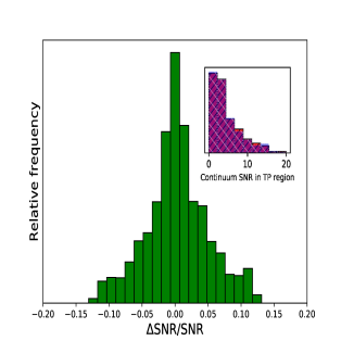
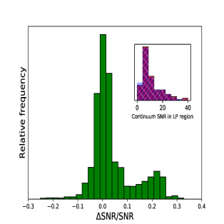
Figure 2.— Left: The histogram plot showing the distribution of $\Delta$SNR/SNR ($\equiv$ [SNR_prox-SNR${}_{\textsc{igm}}$]/SNR_prox) based on the SNR of the spectra of the background quasars (SNR_prox) and the redshift matched control sample (SNR${}_{\textsc{igm}}$). Right: Same as left but from the spectra of the foreground quasars and their corresponding control sample. In the insets, we plot the SNRs of the spectra of quasars in our main sample (white-slanted) and its corresponding control sample (black-slanted) in the proximity region used in our analysis.

2.4. Control sample of Ly$\alpha$ forest

For carrying out the statistical analysis of the Ly$\alpha$ absorption, we use pixel optical depth, $\tau(\lambda_{i})$, statistics (e.g., Rollinde et al., 2005; Dall’Aglio & Gnedin, 2010), where, $\tau(\lambda_{i})=-ln[F(\lambda_{i})/F_{c}(\lambda_{i})]$ is the effective optical depth integrated over the pixel width (69 km s^-1 for SDSS spectra) of the observed spectrum. Here, $F(\lambda_{i})$ and $F_{c}(\lambda_{i})$ are the observed flux and the unabsorbed continuum flux respectively at the $i^{th}$ pixel having a wavelength $\lambda_{i}$. In this method, the proximity effect analysis is carried out by performing a statistical comparison of a probability distribution of pixel optical depth obtained from the proximity region with that originating from the general IGM. However, while combining the optical depths of Ly$\alpha$ absorption from different redshifts it is important to account for the strong redshift evolution of the optical depth.

One possibility is to scale the optical depth measured at various redshifts to their expected value at some fixed reference redshift (e.g., see Rollinde et al., 2005; Dall’Aglio et al., 2008b; Kirkman & Tytler, 2008; Faucher-Giguère et al., 2008b). However, given the fact that the observed optical depth distribution has lower and upper limits based on the noise in the continuum and the core of the saturated absorption lines, such scaling may artificially introduce the pixel optical depth values beyond these observational limits. This may bias the statistics by creating an artificial difference between the pixel optical depth distributions measured for the IGM and the proximity region. This issue is particularly important for our sample as it is based on the SDSS spectra which are obtained with a low/moderate resolution ($R\sim 2000$) and low SNR (mostly $<20$) where the observed line profiles can easily hide the saturated absorption lines.

An alternate approach to the redshift scaling is to use a control sample of Ly$\alpha$ absorption from the IGM. A control sample spectra matching closely in the redshift and in the continuum SNR with that of the spectra of the quasars in our pair sample can be used for studying the proximity effect. Therefore, even though there is redshift evolution of optical depth measured in the proximity regions, a similar evolution will also be present in the control sample of the IGM, which will be used as a comparison sample. We adopt this approach in our analysis. For constructing such a control sample, we made use of the non-BAL quasar catalog from SDSS DR12 after cross-correlating with the DLAs/sub-DLAs catalog of Noterdaeme et al. (2009, 2012) to remove any sightlines with DLA. This sample of quasars without BAL and DLA along their line-of-sight will be referred as IGM parent sample.

To choose SNR matched control sample from this IGM parent sample, consisting of $\sim$ 63,000 quasars, we calculated a running median SNR (continuum/$\langle$error$\rangle$) over a window of 75 pixels in the Ly$\alpha$ forest. These 75 pixels correspond to a radial distance of $\sim$ 15 Mpc at a redshift of $z\sim$ 3 for a spectrum observed with SDSS resolution. The control sample for each sightline of our 181 quasar pairs were generated from the above IGM parent sample, such that $\Delta$SNR/SNR ($\equiv$ [SNR_prox-SNR${}_{\textsc{igm}}$]/SNR_prox) is as small as possible in the spectral range corresponding to the 15 Mpc of the proximity region. Moreover, for reasonably good statistics, we demand 25 quasars as a control sample for each quasar in our pair sample. With these criteria, it can be noted from Fig. 2 that we could achieve $\Delta$SNR/SNR less than $\pm$0.15 for the TPE analysis (using background quasar’s sightlines) and $\pm$0.35 for the LPE analysis (using foreground quasar’s sightlines). In the LPE analysis, due to the presence of strong Ly$\alpha$ emission line, the SNR in the spectral region used for longitudinal proximity analysis is typically high. Therefore, due to the scarcity of high SNR SDSS spectra, we have to allow a larger window of $\Delta$SNR/SNR (i.e., $\pm$ 0.35). We have also ensured non-repetition of sightlines while constructing the control sample for each direction, to remove the possible significant contribution from repeated use of any peculiar sightline.

Furthermore, we checked all the quasar spectra in the control sample, visually, for any peculiarity and LLS in the wavelength region corresponding to the proximity region of the quasar in the 181 quasar pairs sample. This led to the exclusion of just 10 and 7 sightlines from the control sample constructed for TPE and LPE respectively. Using this procedure, we have ensured the exact redshift matching along with a good matching of the continuum SNR between the spectral range used for the proximity analysis and the corresponding spectral range in the control sample (e.g., see Fig. 2). We would like to point out the fact that the IGM region from the control sample is required to be at least 15 Mpc from its emission redshift to avoid its longitudinal proximity region. Therefore, the emission redshift of the control sample may vary from its corresponding proximity sample. In the inset of the Fig. 2, we have shown the SNR of the proximity sightlines and control sample sightlines over the wavelength range used in our analysis. In the upper two panels of Fig. 3, we have shown an example of our high SNR proximity sample and one of its corresponding control sample. A similar plot for the low SNR sightline is shown in Fig. 4. Additionally, we note that the quasars in both the comparison samples in our analysis, viz. pairs sample and the corresponding control sample, were observed in the SDSS using the same spectral setting, as a result, any effect of spectral resolution will also be similar for both of them.

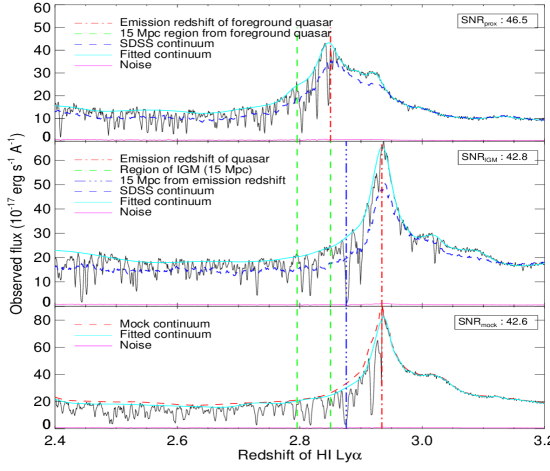
Figure 3.— Upper panel: SDSS spectrum of one of the foreground quasars (J2156+0037) at $z=$ 2.85 (red, dot-dashed vertical line), which has the highest SNR in our sample of the foreground quasars overlaid with the SDSS continuum (blue, dashed) along with our improved continuum, fitted using iterative B-spline fitting method (cyan, solid). The vertical green dashed lines represents the proximity region (15 Mpc) considered in our analysis. The noise spectra is represented with magenta color along with the median SNR (in the proximity region) stated at the upper right corner. Middle panel: Same as the upper panel but for one of the quasars in the corresponding control sample of the above foreground quasar. The red dot-dashed line shows the emission redshift of the control sample while the blue dot-dot-dot-dashed line shows its proximity region. Lower panel: The plot shows the mock spectrum of the quasar used as control sample above, overlaid with the true continuum (red, dashed) along with our fitted continuum (cyan, solid).

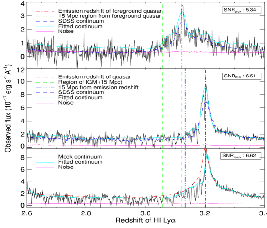
Figure 4.— Same as Fig. 3 but illustrated here by taking an example of a low SNR foreground quasar in our sample (J1111+0613 at $z=$ 3.12).

3. Analysis and results

3.1. Flux and optical depth analysis

The normalized transmitted flux $[F_{t}(\lambda_{i})]$ of a quasar spectrum at i^th pixel having wavelength $\lambda_{i}$ is given by,

$$F_{t}(\lambda_{i})\equiv F(\lambda_{i})/F_{c}(\lambda_{i})=e^{-\tau(\lambda_{i})}$$ (7)

where, $F_{c}(\lambda_{i})$ is the unabsorbed continuum flux fitted to the observed flux $F(\lambda_{i})$ and $\tau(\lambda_{i})$ is the pixel optical depth. We compare the distribution of the normalized transmitted flux as well as of the pixel optical depth measured in the proximity region to that in the SNR and redshift matched spectral region along the line-of-sight to the quasars in the control sample. The continuum placement in the Ly$\alpha$ forest and its associated uncertainty can have a significant impact on both the transmitted flux and the optical depth statistics, which we have investigated with a detailed analysis in the next subsection.

3.1.1 Quasar continuum normalization and it’s uncertainty

During our visual inspection, we noticed that the continuum fit given by SDSS DR12 pipeline systematically underestimates the continuum flux especially in the Ly$\alpha$ forest as evident from top panels of Fig. 3 and Fig. 4 for it’s illustration in a high and low SNR spectrum respectively (see also Lee et al., 2012). Therefore, we have refitted the continuum for all quasar spectra used in our study. For this, we have used iterative B-spline fitting along with the median smoothing function by optimizing the fitting parameters interactively to get the best continuum fit. The procedure adopted here is similar to that of Dall’Aglio et al. (2008a, b). As a first step, we divide the whole spectrum into small intervals such that the emission line region has a smaller interval length to take into account a large flux gradient over this region. Each of these small chunks of wavelength versus flux are then fitted by an iterative B-spline fitting algorithm. The order of the fitted B-spline does vary among various quasar spectra but in most of the cases, a $4^{th}$ order has resulted in an optimal fit. Secondly, we minimize the $\chi^{2}$ between the flux spectrum and our modelled continuum in each chunk of the spectrum iteratively. In each iteration, a certain number of pixels got rejected which lies outside the range of our allowed 3$\sigma$ significance level, leading to the removal of high absorption pixels iteratively in each chunk. The full continuum is then the smoothed function of the fitted continuum to these chunks. This leads to an improved continuum fit to all quasar spectra used in this study as compared to the default SDSS continuum as shown in the top panels of Fig. 3 (e.g., for high SNR spectrum) and Fig. 4 (e.g., for low SNR spectrum).

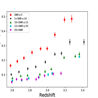
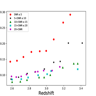
Figure 5.— Left panel: The plot shows median value of continuum shifts $\langle\Delta C/C\rangle$ versus redshift measured in various SNR bins using the mock spectra from Bautista et al. (2015). The error bars on the mean shift plotted here are enhanced by a factor of 9, which otherwise are smaller than the symbol size. We have incorporated such continuum shift in our analysis (e.g., see Sect. 3.1.1). It can be seen from the figure that as expected based on the redshift evolution of Ly$\alpha$ optical depth, the $\langle\Delta C/C\rangle$ at a given SNR increases with increasing $z$. The effect seems stronger for the lower SNR. Right panel: The plot shows the median value of the fractional uncertainty in the continuum ($\sigma[\Delta\textsc{c/c}]$) versus the redshift measured in the various SNR bins using the mock spectra from Bautista et al. (2015).

However, due to numerous absorption lines in the Ly$\alpha$ forest, a systematic continuum placement error may still remain (particularly for low SNR spectra). To quantify this, we have used the mock quasar spectra simulated by Bautista et al. (2015). They have obtained the mock spectrum in three steps: Firstly, they generated the Ly$\alpha$ optical depth values along the line-of-sight. Then this simulated normalized flux ($F=e^{-\tau}$) is multiplied by a synthetic quasar continuum flux ($F_{c}$). Secondly, the mock spectra are convolved with the kernel to have a similar resolution ($R\sim 2000$). Furthermore, they have also ensured that mock quasar has emission redshift, the mean flux in the Ly$\alpha$ forest and a spectral index similar to those of the corresponding real quasar found in SDSS DR11 quasar catalog. Finally, instrumental noise, metal lines, high column density absorbers and other potential sources of systematics are added to the spectrum to match statistically with the real SDSS quasar spectrum. The noise added to the fluxes of a given mock quasar is a random number from a Gaussian distribution of mean zero with a variance determined by the noise model for the corresponding real quasar. In the bottom panels of Fig. 3 and Fig. 4, we have shown the mock spectrum for the corresponding IGM control sample plotted in the middle panels. For each real spectrum in our sample, we took 100 such realizations of its mock spectra from Bautista et al. (2015).

We fitted the continuum to all these mock spectra using our continuum fitting procedure. This allows us to compute the fractional uncertainty between the true ($C_{t}$, red-dashed line of bottom panels of Figs. 3, 4) and the fitted continuum ($C_{f}$, cyan-solid line of bottom panels of Figs. 3, 4) over the wavelength range relevant for our proximity analysis (i.e., within vertical green-dashed line of Figs. 3, 4), viz., $\Delta C/C~{}\equiv~{}[C_{t}-C_{f}]/C_{f}$, for each pixel. The mean of this distribution ($\langle\Delta C/C\rangle$) is used to apply a systematic continuum shift in all the pixels of the proximity region to obtain the unabsorbed intrinsic continuum ($F_{c}[\lambda_{i}]$) as,

$$F_{c}[\lambda_{i}]=C_{f}[\lambda_{i}]\times(1+\langle\Delta C/C\rangle).$$ (8)

The typical uncertainty in the continuum flux is computed using the standard deviation ($\sigma[\Delta\textsc{c/c}]$) of this $\Delta C/C$ distribution as follows,

$$\delta F_{c}[\lambda_{i}]=\sigma[\Delta\textsc{c/c}]C_{f}[\lambda_{i}]\times\Big{(}1+\langle\Delta C/C\rangle\Big{)}$$ (9)

Here, we have neglected the error on the mean value of $\Delta C/C$ as it is found to be negligible compared to the above systematic continuum error.

The mock spectra were available for about 67% of the total quasar sightlines used in our analysis. The unavailability of the mock spectra for the remaining 33% sightlines is probably due to the fact that Bautista et al. (2015) has confined their study only to the quasars catalog of SDSS DR11. However, our sample (both quasar pairs and control sample) is based on SDSS DR12 quasars catalog which has added a substantial number of new quasars beside including the quasars from SDSS DR11 quasars catalog. For these remaining 33% quasar sightlines without the mock spectra, we have applied the continuum correction by using the shift based on those mock spectra which are closely matching in the SNR and the redshift.

The fractional averaged systematic continuum shift (i.e., $\langle\Delta C/C\rangle$) and the typical continuum uncertainty per pixel as a function of redshift is plotted in the left and right panel of Fig. 5 respectively, for various SNR bins. As can be seen from the figure that, (i) as the SNR increases, the fractional systematic continuum shift decreases and (ii) there seem to be a moderate increasing trend with the redshift for higher SNR bins in comparison to a strong increasing trend apparent for lower SNR bins. The typical continuum uncertainty also follows similar trend except for very high SNR bin. In very high SNR bin, our continuum procedure optimized for moderate SNR spectra may start tracing the absorption, leading to higher uncertainty. This shows the importance of applying the continuum correction along with the proper estimation of its uncertainty computed for individual sightline. In our analysis that follows, we use the corrected continuum flux (e.g., see, Eq. 8) for each sightline along with the error spectrum (e.g., see, Eq. 9). This will allow us to include the continuum placement uncertainties in the normalized transmitted flux (e.g., see, Eq. 7) along with the other measured flux uncertainties at each pixel as discussed in the next subsection.

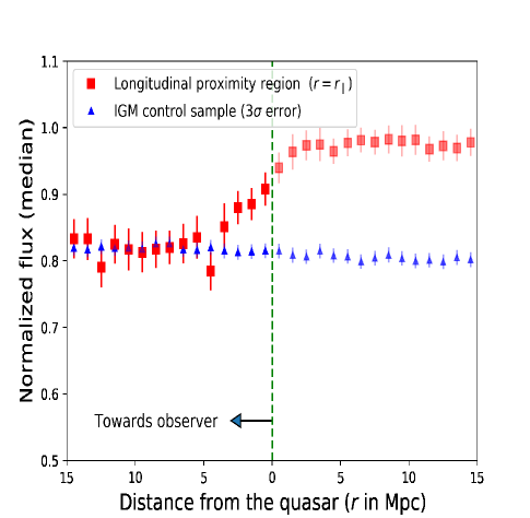
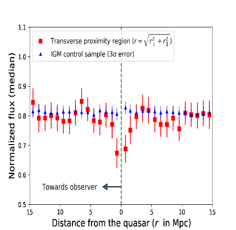
Figure 6.— The plots show median transmitted flux in different radial distance bins from the foreground quasars for the longitudinal (left) and the transverse proximity regions (right). The plots also show the corresponding median transmitted flux for the control sample (blue, triangle) selected based on appropriate matching of the redshift and SNR in the proximity region (i.e., LPE and TPE of our foreground quasars) of our main sample (e.g., see Sect. 2.4). For the LPE (left panel) it may be noted that the quasar’s continuum flux beyond Ly$\alpha$ emission line is shown in fainter color to distinguish them from real Ly$\alpha$ absorption. In this plot, the error bars on the median transmitted flux of the proximity region consists of flux error from photon counting statistics, error due to the continuum placement uncertainties, r.m.s statistical errors, sightline-to-sightline variance and emission redshift measurement error within the 1 Mpc radial distance bin (e.g., Sect. 3.1.2), whereas for control sample only the former three error contributes. Here, the error-bars in the control sample are smaller than the symbol size due to statistics of large numbers (being $\sim$ 25 IGM sightlines per quasar sightline). Therefore, we have plotted the 3$\sigma$ error for the IGM median flux. The green dashed line shows the location of the foreground quasar.

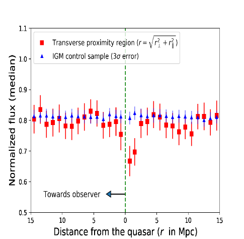
Figure 7.— Same as Fig. 6 except that here we have not applied the systematic redshift uncertainty correction of 229 km s^-1 to the emission redshift of the foreground quasar (e.g., see Sect. 2.2) leading to an asymmetry among blueward and redward of the foreground quasar as evident in the transverse direction.

3.1.2 Transmitted flux uncertainties

To quantify the difference in $F_{t}$ (e.g., see, Eq. 7) for a given radial distance bin of the proximity region as compared to its control sample, it is important to carefully consider all the probable sources of uncertainties involved in the measurement of the median $F_{t}$. In our analysis, the first contribution of error ($\Delta F^{fc}_{t}$) in the normalized spectrum comes from the propagation of flux measurement errors and continuum placement uncertainties at each pixel, which is computed as follows,

$$\Delta F^{fc}_{t}[\lambda_{i}]=F_{t}[\lambda_{i}]\times\sqrt{\Bigg{(}\frac{\delta F[\lambda_{i}]}{F[\lambda_{i}]}\Bigg{)}^{2}+\Bigg{(}\frac{\delta F_{c}[\lambda_{i}]}{F_{c}[\lambda_{i}]}\Bigg{)}^{2}}.$$

Here, $\delta F_{c}[\lambda_{i}]$ is the error introduced due to the continuum fitting uncertainties derived using mock spectra (e.g., see Eq. 9) for a given $F_{c}[\lambda_{i}]$ (e.g., see Eq. 8) at the $i^{th}$ pixel with wavelength $\lambda_{i}$. $\delta F[\lambda_{i}]$ is the error on the flux measurement $F[\lambda_{i}]$ provided by the SDSS pipeline. Therefore, the error on the mean transmitted flux (from all the 181 spectra) in a radial distance bin is obtained using,

$$\Delta F^{fc}_{t}=\Bigg{[}\frac{\sum_{j=1}^{N_{spec}}\sum_{i=1}^{N_{j}}F^{j}_{t}[\lambda_{i}]^{2}\times\Big{(}\frac{\delta F^{j}[\lambda_{i}]}{F^{j}[\lambda_{i}]}\Big{)}^{2}}{(\sum_{j=1}^{N_{spec}}N^{j})^{2}}\\ +\frac{\sum_{j=1}^{N_{spec}}\sum_{i=1}^{N_{j}}F^{j}_{t}[\lambda_{i}]^{2}\times\Big{(}\frac{\delta F_{c}^{j}[\lambda_{i}]}{F_{c}^{j}[\lambda_{i}]}\Big{)}^{2}}{(N_{spec})^{2}}\Bigg{]}^{1/2}$$ (10)

The first and the second term are the photon counting noise and the continuum placement error respectively. N_spec is the number of spectra i.e., 181 and N_j is the number of the pixels in the j^th spectrum used within the radial distance bin of size 1 Mpc (typically 4-6 pixels). Here, it may be noted that the continuum placement error in a given spectrum might be correlated. We have taken this into account by averaging it over only the number of spectra (expected to be uncorrelated) instead of averaging it over the total number of the pixels in a given radial distance bin (e.g., see the second term).

Second contribution to the error in the normalized flux is due to the dispersion of $F_{t}$ among the various pixels around its median value in a given radial distance bin (i.e., r.m.s. scatter, $\Delta F^{rms}_{t}$). This r.m.s. scatter is calculated as

$$\Delta F^{rms}_{t}=\frac{\sqrt{\sum_{i=0}^{N}[{F_{t}(i)-\langle F_{t}\rangle}]^{2}}}{N}.$$ (11)

Here, $N=\sum_{j=1}^{N_{spec}}{N_{j}}$, is the total number of the pixels in 1 Mpc radial bin.

Third contribution to the total error budget is due to the sightline-to-sightline variance of the sample ($\Delta F^{var}_{t}$). For this, we have used the empirical bootstrap technique (e.g., see Efron & J. Tibshirani, 1993). In this method, we constructed a new sample of 181 quasars proximity sightlines by randomly selecting them from our original dataset of 181 quasars (i.e., allowing a random exclusion of sightlines at the cost of the equal number of random repetition of some other sightlines). The histogram of the median transmitted flux of 100 such realizations, within the spectral range corresponding to 1 Mpc spatial separation (i.e., radial bins corresponding to the proximity region), are well fitted with a Gaussian profile. This results in an average standard deviation in the transmitted flux of $\sim$ 2% per 1 Mpc radial distance bin (varying within the range of $1.0\%$ to $3.0\%$ in different radial distance bins). This standard deviation has been used to include the sightline-to-sightline variance in our final error budget.

Lastly, we also included the uncertainty in the median $F_{t}$ measured in the proximity region due to the typical emission redshift uncertainty ($\Delta F^{z}_{t}$) of $\sim$ 330 km s^-1 along our sightlines as discussed in Sect. 2.2. For this, we have carried out an analysis of 100 realizations by adding a random velocity offset (with Gaussian distribution) to the individual quasar redshifts within $\pm$330 km s^-1 range. This offset in the redshift will propagate by affecting the inferred distance between the quasar and the absorber in the form of the number of pixels to be considered in a given radial distance bin. As a result, the corresponding uncertainty in the $F_{t}$ is estimated based on the spread of the measured median $F_{t}$ among these 100 realizations, for each radial distance bin.

Therefore, the total error on the transmitted flux of the proximity region ($\Delta F^{prox}_{t}$) for a given radial distance bin is the quadratic sum of all the above-mentioned errors (e.g., see Eqs. 9, 10 and 11),

$$\Delta F^{prox}_{t}=\sqrt{(\Delta F^{fc}_{t})^{2}+(\Delta F^{rms}_{t})^{2}+(\Delta F^{var}_{t})^{2}+(\Delta F^{z}_{t})^{2}}.$$ (12)

Similar treatment on the error budget is carried out for the estimation of error in the flux from the control sample except that $\Delta F^{var}_{t}$ and $\Delta F^{z}_{t}$ are ignored here. The $\Delta F^{z}_{t}$ does not exists for IGM and $\Delta F^{var}_{t}$ is negligible due to large statistics, having $\sim$ 25 quasars in the control sample for each member of the pair in our sample. Therefore, the total error on the transmitted flux from the control sample ($\Delta F^{\textsc{igm}}_{t}$) in a given radial distance bin is,

$$\Delta F^{\textsc{igm}}_{t}=\sqrt{(\Delta F^{fc}_{t})^{2}+(\Delta F^{rms}_{t})^{2}}.$$ (13)

After taking into account all these uncertainties, we can compare the transmitted flux in the longitudinal and transverse directions to that in their corresponding control sample, as explained below.

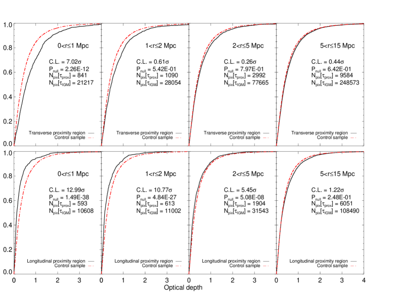
Figure 8.— Upper panels: The cumulative probability distribution function (CPDF) of H i Ly$\alpha$ optical depth in the transverse proximity regions (black-solid) at different radial distances from the foreground quasar together with the optical depth CPDF from the control sample (red-dashed). Labels in each panel give the range of radial distance from the foreground quasars used to make the subsample for these CPDFs of pixel optical depth (see, Sect. 3.1.4 for more details). The uncertainty in the optical depth at each pixel in the proximity region is used to estimate the typical error in the KS-distance measurement of KS-test and hence the corresponding confidence level (C.L.) as well as the null probability (P_null) on the measured difference in the CPDFs as labeled in each panel (e.g., see Sect. 3.1.4). The number of pixels used in the CPDFs of the proximity region (N${}_{pix}[\tau_{prox}$]) and control sample (N${}_{pix}[\tau_{\textsc{igm}}$]) are also mentioned. Lower panels: Same as the top panels but for the longitudinal proximity region.

3.1.3 Transmitted flux statistics

In Fig. 6, we plot median values of the normalized transmitted flux, $F_{t}$ (within 1 Mpc radial distance bin) at various radial distances from the quasars in both longitudinal and transverse directions, towards observer and towards background quasar of the foreground quasar. The procedure is similar to that given by Kirkman & Tytler (2008) where they plot $1-F_{t}$ in the proximity region of the foreground quasar.

As a consistency check, it can be seen from the Fig. 6 that the values of median $F_{t}$ at different radial distance bins are almost constant (within their uncertainties) for both the control samples used in the LPE and TPE analysis. Furthermore, it can also be noted that $F_{t}$ measured in the proximity region is consistent with that from the control sample at large radial distances (as expected) with its median value of $\sim$ 0.80. It may be pointed out that in each radial distance bin, we have lumped together the pixels over the redshift range of $\sim$ 2.5 to 3.5 due to scatter in the $z_{f}$ without accounting for the existing optical depth redshift evolution. However, we stress that our appropriate selection of the redshift matched control samples (e.g., see Sect. 2.4) take care of such effects due to its similar redshift evolution.

From Fig. 6, we can see the difference in $F_{t}$ among the longitudinal (left panel) and the transverse (right panel) directions. It can be seen from the left-hand panel of this figure that there is a clear increase of the transmitted flux as we go closer to the quasar ($r\leq 4$ Mpc, towards to observer) in the longitudinal direction as compared to its control sample. This hints towards the dominance of the quasars ionization, as expected in the classical proximity effect, at smaller radial distances. Note, Kirkman & Tytler (2008) did not detect such a signal of the longitudinal proximity effect. It can be noted from this figure that the transmitted flux redward of the Ly$\alpha$ emission (shown by fainter color) in the first three radial distance bins (i.e., $0\leq r\leq 3$ Mpc) show nominal absorption features. Such absorption could arise due to the possible redshift uncertainty (even after incorporating the average systematic redshift correction, e.g., see Sect. 2.2) and/or the possible inflow of the Ly$\alpha$ clouds towards the center of quasar’s halo (resulting in the redshift of such clouds to be more than the emission redshift of the foreground quasars). At higher radial bin (i.e., $r>3$ Mpc) the transmitted flux is close to unity albeit a small systematic decrement of about 2%, similar to the residual absorption found in this region by Kirkman & Tytler (2008) where they have ascribed it to metal absorption. Nonetheless, we still checked this region visually to ensure that continuum is not systematically overestimated in individual spectra.

However, from our analysis in the transverse direction, this trend appears to be reversed, especially within 2 Mpc radial distance blueward and redward of the foreground quasar Ly$\alpha$ emission line. This clearly suggests the presence of excess H i absorption closer to the quasar in the transverse direction likely due to less illumination in this direction (e.g., see Sect. 3.2).

Additionally, we may also recall that in our emission redshift estimation we have added a systematic shift of 229 km s^-1 (as estimated by Shen et al., 2016) so it will be interesting to see its impact on the above analysis. For this, we have repeated our analysis by using emission redshift without applying this systematic shift as shown in Fig. 7. As can be seen from this figure that a clear asymmetry in H i absorption is evident between the absorption profile blueward and redward of the foreground quasar in the transverse direction. Such asymmetry could be easily misinterpreted as a consequence of a possible episodic lifetime of the quasars (e.g., see Kirkman & Tytler, 2008; Khrykin et al., 2016). Additionally, a consonance may be noted between the systematic shift of 229 km s^-1 in the emission redshift provided by Shen et al. (2016) from an independent method to the exact symmetric H i absorption profile measured in the transverse direction (when correction is applied). In what follows, we always use the emission redshifts corrected for the above mentioned systematic uncertainty.

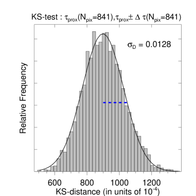
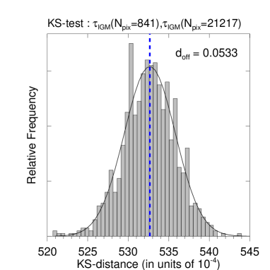
Figure 9.— Upper panel: The plot shows the distribution of the KS-distance values obtained by comparing the CPDF of the pixel optical depth of the proximity region ($\tau_{prox}$) with its 5000 realizations ($\tau_{prox}\pm\Delta\tau$), generated assuming the Gaussian distribution at each pixel, with a width corresponding to the error bars of the pixel optical depth. The plotted distribution of the measured KS-distances allows us to compute its standard deviation ($\sigma_{\textsc{d}}$). Lower panel: The plot shows the distribution of the KS-distance values obtained by comparing the CPDF of the pixel optical depth of the parent sample of the IGM ($\tau_{\textsc{igm}}[N_{pix}=21217]$) with its 1000 random subsets ($\tau_{\textsc{igm}}[N_{pix}=841]$). The number of pixels in each of the subset is set to be equal to the number of pixels available in their corresponding proximity sample. The plotted distribution of the measured KS-distances allows us to compute its mean value (d_off), used to apply the offset correction in the measured KS-distance between the proximity vis-a-vis the IGM distribution and hence the confidence level as [D_ks-d_off]/$\sigma_{\textsc{d}}$.

3.1.4 Pixel optical depth statistics

We use the values of fluxes used to obtain median fluxes plotted in Fig. 6, to compute the optical depth as $\tau(\lambda_{i})=-ln[F_{t}(\lambda_{i})]$ (e.g., see Eq. 7) for our subsequent pixel optical depth analysis. The pixel optical depth we obtain is an integrated value over the pixel width (i.e., $\sim$ 69 km s^-1 in our SDSS spectra having $R\sim$ 2000). Using these pixel optical depth values, we have computed the cumulative probability distribution function (CPDF) as shown in Fig. 8. The figure compares the CPDFs of the optical depth in the proximity region with that of the control sample within the radial distance bins of 0-1, 1-2, 2-5 and 5-15 Mpc. As can be seen from this figure that the form of the optical depth distribution in the proximity region is similar to the distribution in the control sample. However, its value in the transverse proximity region is higher than its control sample (e.g., see upper panel), while the trend seems to be reversed in the longitudinal direction (e.g., see lower panel), at least up to the radial distance of $\leq 5$ Mpc from the ionizing foreground quasar.

To quantify the difference evident in the CPDFs of the proximity and the corresponding control sample, we have used the Kolmogorov-Smirnov (KS) test. This allows us to compute the KS-distance (D_ks) and the probability for the two distributions to be the same (P_null). However, we note that the P_null and D_ks estimated in the standard KS-test does not take into account the uncertainties on the pixel optical depth and hence may lead to an overestimation of the significance level of any difference among the two CPDFs. The resultant distortion introduced by such uncertainties can be significant for the optical depth CPDFs of the proximity region due to its small statistics, though any such effect will be negligible in the control sample having larger statistics (being $\sim$ 25 times that of proximity region). Therefore, to be on the conservative side, instead of using the standard KS-test, we have estimated the significance of the measured D_ks and P_null by taking into account the uncertainties in the optical depth of the proximity region (as also used in Fig. 7), as follows.

We assume the measured value of the optical depth and its uncertainties at a pixel as a mean and 1$\sigma$ width of a Gaussian distribution of the optical depth at that pixel. Then using this distribution, 5000 random values of optical depth are generated at each pixel. The distribution of KS-distance values obtained by comparing the CPDFs of these 5000 realizations with the original CPDF of the proximity region is found to be well-fitted with a Gaussian profile. The upper panel of Fig. 9 shows an example of one such distribution of KS-distance values for a radial distance bin. The 1$\sigma$ width of this KS-distance distribution, $\sigma_{\textsc{d}}$, is considered as a typical uncertainty in the measured D_ks. Now, in principle, the ratio of the D_ks and $\sigma_{\textsc{d}}$ can be used to determine the confidence level, however, we noticed that the measured mean value of KS-distance has a non-zero offset when we compare two distributions with a different number of data points, even when they are drawn from the same parent distribution. Such an offset can artificially lead to an over-estimation of the confidence level based on the ratio of the D_ks and $\sigma_{\textsc{d}}$. In order to account for this bias, we use the control sample and compare it with its own random subsamples. These random subsamples are constructed with a constraint that the number of pixels in these subsamples should be equal to that in their corresponding proximity sample.

Using the comparison of such 1000 subsamples with their own parent control sample, we computed the mean KS-distance offset (d_off). An example of one such distribution of KS-distance values to compute $d_{off}$ is plotted in the lower panel of Fig. 9. This allows us to compute the accurate confidence level (C.L.) as [D_ks-d_off]/$\sigma_{\textsc{d}}$ and P_null as the area under the normalized Gaussian curve of standard deviation $\sigma_{\textsc{d}}$ beyond $\pm$[D_ks-d_off] range, as labeled in each panel of the Fig. 8. It can be noted from the figure that in the transverse direction the measured optical depth in the proximity region is higher than the control sample in 0-1 Mpc radial bin at a significance of 7.02$\sigma$. Also, while plotting the CPDF for the transverse direction, we have lumped together the absorption systems in blueward and redward of the foreground quasar Ly$\alpha$ emission line. The difference in the longitudinal direction is also significant (e.g., see lower panel), though have an opposite trend with being smaller in the proximity region than in the control sample at 12.99$\sigma$ and 10.77$\sigma$ in the radial bins of 0-1 and 1-2 Mpc respectively.

This dissimilarity of the CPDFs of the optical depth in the transverse and the longitudinal directions indicates that the observed optical depth distribution around the quasar may be anisotropic. This is consistent with the inference drawn based on the transmitted flux statistics (e.g., see Fig. 6). This anisotropic distribution could result from an anisotropic radiation field from the quasars or anisotropic matter distribution around them. However, before interpreting the difference seen in the CPDFs, the value of optical depth at a given pixel should be corrected for the effect of quasar’s ionizing radiation as we describe in the next subsection.

3.2. Ionization and overdensity effects in the proximity region

From our analysis of the transmitted flux (e.g., see Fig. 6) and the pixel optical depth distributions (e.g., see Fig. 8) it is evident that these quantities distribute differently along the transverse and the longitudinal directions. The role of anisotropic matter distribution causing this observed difference seems to be unlikely because we have used a large sample of quasars that can lead to an average density profile being isotropic around the quasar. Based on this, we can ascribe the differences we find to anisotropy in the quasar ionization. To quantify this anisotropic distribution, we will first estimate the quasar’s ionization based on the observed flux in the longitudinal direction to get the ionization corrected pixel optical depth distribution. This will enable us to estimate the ionization corrected average excess overdensity profile in the longitudinal direction. Then, we will be keeping the fraction of quasar’s illumination in the transverse direction compared to the longitudinal direction as a free parameter and constrain its best fit value by ensuring a statistical match of the ionization corrected average excess overdensity profile in these two directions.

To estimate the quasar’s ionization, we note that its extent on the observed transmitted flux and pixel optical depth will also be influenced by the strength of the UVB radiation, along with the amount of clustering of matter around quasars expressed in terms of overdensity at a given radial distance bin from the quasar. To lift this degeneracy, we estimated the excess ionization by the quasar relative to the UVB radiation at each radial distance, $r$, from the quasar by computing a scaling factor of $[1+\omega_{r}]$ defined as

$$\frac{\Gamma_{\textsc{uvb}}(z_{a})+\Gamma_{q}(r,z_{a})}{\Gamma_{\textsc{uvb}}(z_{a})}\equiv 1+\omega_{r}$$ (14)

where, $\Gamma_{\textsc{uvb}}(z_{a})$ and $\Gamma_{q}(r,z_{a})$ are the H i photoionization rates at the absorbing cloud at redshift $z_{a}$ contributed by the UVB and quasar respectively. The $\Gamma_{\textsc{uvb}}$ is defined by

$$\Gamma_{\textsc{uvb}}(z_{a})=\int^{\infty}_{\nu_{912}}\frac{4\pi J_{\nu}(z_{a})}{h\nu}\sigma_{HI}d\nu$$ (15)

where, $J_{\nu}$ is the average specific intensity of UVB (in units of erg cm^-2 s^-1 Hz^-1 sr^-1), $\nu_{912}$ is the frequency corresponding to 912 Å (i.e., H i ionizing energy) and $\sigma_{HI}$ is the photoionization cross-section given by

$$\sigma_{HI}=\sigma_{0}\left(\frac{\nu}{\nu_{912}}\right)^{-3}$$ (16)

with $\sigma_{0}=6.30\times 10^{-18}$ cm² (e.g., Osterbrock & Ferland, 2006). We used the value of $\Gamma_{\textsc{uvb}}(z)$ given by Khaire & Srianand (2015a) based on their updated estimation of $J_{\nu}$ using comoving specific galaxy and quasar emissivities at different redshifts. The $\Gamma_{q}$ is given by,

$$\Gamma_{q}(r,z_{a})=\int^{\infty}_{\nu_{912}}\frac{L_{\nu}}{4\pi r^{2}}\frac{\sigma_{HI}}{h\nu}d\nu$$ (17)

where, $r$ is the distance of the absorbing cloud at $z_{a}$ from the foreground quasar at $z_{f}$ (e.g., see Eq. 2) with luminosity $L_{\nu}$ (in units of erg s^-1 Hz^-1) calculated by Eq. 5 and Eq. 6. Integrating, the above equation results in,

$$\Gamma_{q}(r,z_{a})\\ =\frac{\sigma_{0}~{}L_{\nu_{1325}}}{4\pi r^{2}h(3+\alpha_{uv})}\left(\frac{\nu_{1300}}{\nu_{1325}}\right)^{-\alpha}\left(\frac{\nu_{912}}{\nu_{1300}}\right)^{-\alpha_{uv}}$$ (18)

where, $h$ is the Planck’s constant. With our estimation of $\Gamma_{q}(r,z_{a})$ and $\Gamma_{\textsc{uvb}}(z_{a})$, we can compute $[1+\omega_{r}]$ scaling factor to compensate for the decrement of the optical depth due to the excess ionization (e.g., see Rollinde et al., 2005; Faucher-Giguère et al., 2008a) as,

$$\tau_{off}=[1+\omega_{r}]\times\tau_{prox}$$ (19)

where, $\tau_{off}$ is the optical depth that would be obtained if the quasar was turned off and $\tau_{prox}$ is the measured optical depth in the presence of the quasar. However, such [$1+\omega_{r}$] scaling for $\tau_{prox}$ is valid for high-resolution spectra and may not be valid in the case of the SDSS spectra where the measured optical depth does not necessarily follow the column density due to poor spectral resolution (e.g., see Lee et al., 2012). Therefore, it is essential to carry out a quantitative analysis on the validity of such scaling at low/moderate resolution using simulated spectra. For this purpose, we generated simulated spectra based on numerical simulation to quantify a scaling relation of the form as,

$$\tau_{off}=[1+\omega^{ef}_{r}(\tau,\omega_{r})]\times\tau_{prox}.$$ (20)

Here, $[1+\omega^{ef}_{r}(\tau,\omega_{r})]$ is an effective optimized scaling for low/moderate resolution spectra instead of the [$1+\omega_{r}$] scaling such that,

$$\bigg{[}\frac{\Gamma_{\textsc{uvb}}(z_{a})+\Gamma_{q}(r,z_{a})}{\Gamma_{\textsc{uvb}}(z_{a})}\bigg{]}^{ef}\equiv 1+\omega^{ef}_{r}(\tau,\omega_{r})$$ (21)

In addition, quasars may also reside in an overdense region (e.g., see Rollinde et al., 2005; Kirkman & Tytler, 2008; Finley et al., 2014; Adams et al., 2015; Lau et al., 2018). Therefore, contrary to the expected decrease in the optical depth due to extra ionization by the quasar’s radiation this overdensity will lead to an increase of the observed effective optical depth in the proximity region as described below.

The photoionization equilibrium, for a highly ionized optically thin gas is given by,

$$n_{\textsc{Hi}}\Gamma_{\textsc{Hi}}=R(T[\Delta])~{}n_{e}n_{\textsc{Hii}}\approx Rn^{2}_{\textsc{Hii}}$$ (22)

where, $R(T[\Delta])=4.2\times 10^{-13}(T(\Delta)/10^{4}K)^{-0.7}$ cm³ s^-1 is the recombination rate (e.g., Hui et al., 1997b) and $T(\Delta)=T_{0}\Delta^{\gamma-1}$ is the temperature of the gas having an overdensity $\Delta=\rho(r)/\overline{\rho}$ with an exponent $\gamma$. Here, we have neglected the helium contribution to the free electron density which typically amounts to an error of 8% on $n_{e}$ as estimated by Faucher-Giguère et al. (2008a) for singly ionized helium.

The density of ionized hydrogen ($n_{\textsc{Hii}}$) will be the product of the total hydrogen number density ($n_{H}$) and the fraction of ionized hydrogen ($X_{\textsc{Hii}}$) i.e., $n_{\textsc{Hii}}=n_{H}X_{\textsc{Hii}}$ with $n_{H}=\bar{n}_{H}\Delta$. As we know, $\tau_{\textsc{Hi}}\propto n_{\textsc{Hi}}$ which for a given $\Gamma_{\textsc{Hi}}$ will be proportional to the product of $R(T[\Delta])$ and $\Delta^{2}$ resulting in

$$\tau\propto n_{\textsc{Hi}}\propto T^{-0.7}\Delta^{2}\propto\Delta^{2-0.7(\gamma-1)}.$$ (23)

The combined effect of such a density enhancement and extra ionizing photons around quasars (discussed above, e.g., see Eq. 20), is to shift the observed optical depth in the proximity region $\tau_{prox}$. Following approach similar to Rollinde et al. (2005) and using Eq. 20, we quantify this shift for the measured optical depth in our SDSS spectra as,

$$\tau_{\textsc{igm}}=\tau_{prox}\,\frac{[1+\omega^{ef}_{r}(\tau,\omega_{r})]}{\left(\rho(r)/\overline{\rho}\right)^{2-0.7(\gamma-1)}}.$$ (24)

Therefore, the ratio of $\tau_{prox}\times[1+\omega^{ef}_{r}(\tau,\omega_{r})]/\tau_{\textsc{igm}}$ in various radial bins will allow us to estimate an average excess overdensity profile around the quasars in the longitudinal direction (e.g., see Eq. 24). The corresponding density profile for the transverse direction will be given by $\tau_{prox}\times[1+\omega^{ef}_{r}(\tau,\eta\omega_{r})]/\tau_{\textsc{igm}}$ where, $\eta$ is the fraction of the illumination in the transverse direction as compared to the longitudinal direction (with maximum range of $0\leq\eta\leq 1$). The best fit value of $\eta$ is obtained by $\chi^{2}$ minimization between the average excess overdensity profile in the longitudinal direction and transverse direction as discussed in subsequent subsections (e.g., see Sect. 3.2.2). Here, we may recall that the observed optical depth in the transverse direction is already higher than in the longitudinal direction, therefore, $\eta>1$ will not be consistent with our assumption of the spherically symmetric distribution of matter around the quasar. Before that we first quantify in the next subsection, the scaling factor [$1+\omega^{ef}_{r}(\tau,\omega_{r})$] that is required to estimate the appropriate ionization correction for scaling the optical depth measured in the low/moderate resolution SDSS spectra as a function of $\omega_{r}$ and $\tau_{prox}$.

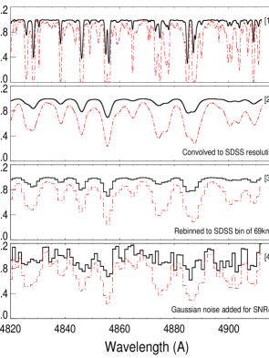
Figure 10.— Panel [1]: Transmitted flux along a line of sight in our simulation box with the gas being ionized by the UVB (red dotted) and excess radiation from a nearby ionizing source (i.e., UVB and quasar, black solid). The additional quasar ionization effect is mimicked by scaling down the optical depth in each pixel by a factor $[1+\omega_{r}]\approx 11$. Panel [2]: This panel shows the spectra displayed in the panel [1] after its convolution with a Gaussian function having FWHM corresponding to the SDSS resolution of $R\sim 2000$. Panel [3]: This panel shows re-binning of the spectra in the panel [2] to a SDSS pixel width of 69 km s^-1. Panel [4]: This panel shows the spectra of the panel [3] after adding a random Gaussian noise corresponding to a typical SNR ($\approx 10$) of our real SDSS spectra.

3.2.1 Appropriate ionization corrections for moderate resolution spectra

We have used the hydrodynamical simulations of IGM, as discussed in details by Gaikwad et al. (2018). In brief, the simulated spectra are obtained by shooting sightlines through the simulated box of size $\sim$ 14 Mpc (comoving) having $2\times 512^{3}$ number of particles. This small box size might amount to assume no spatial correlations of the optical depth between the various radial distance bins. However, its impact may not be significant as our aim here is to validate the ionization scaling only for an effective pixel optical depth value instead for an optical depth distribution. We generated 200 realizations of Ly$\alpha$ optical depth ($\tau_{true}$) as a function of wavelength at a median redshift of 2.5 and 3.0 (e.g., see panel [1] of Fig. 10, red-dotted line). Using these simulated spectra, we estimated the optimal ionization scaling (e.g., see Eq. 20) that is appropriate for our low/moderate resolution SDSS spectra as follows:

1. We have used the simulated pixel optical depth ($\tau_{true}$, e.g., see panel [1] of Fig. 10, red-dotted line) to generate the mock spectra at the SDSS resolution ($\tau_{\textsc{igm}}$). For this, we first convolve the simulated spectrum (i.e., $e^{-[\tau_{true}]}$) with a Gaussian function having a FWHM corresponding to the SDSS resolution of $R\sim 2000$ (e.g., see panel [2] of Fig. 10, red-dotted line). Secondly, we re-bin this convolved spectrum at 69 km s^-1 interval corresponding to the SDSS pixel width (e.g., see panel [3] of Fig. 10, red-dotted line). Thirdly, to mimic the noise of the real spectrum, we added a random Gaussian noise (e.g., see panel [4] of Fig. 10, red-dotted line) with a mean of zero and a standard deviation of 1/SNR.

2. To generate the optical depth distribution as observed after excess ionization due to the quasar observed in a low resolution spectrum ($\tau_{prox}$), we follow the same steps as listed above (i.e., point [1]) except that instead of using $\tau_{true}$, we have used $\tau_{true}/[1+\omega_{r}]$ for a given input $\omega_{r}$ (e.g., see Eq. 14) as shown by black-solid line in panels [1]-[4] of Fig. 10.

3. We noticed that in order to recover the $\tau_{\textsc{igm}}$ from its corresponding ionized pixels $\tau_{prox}$ (for a given $\omega_{r}$) at the SDSS resolution, the required ionization correction i.e., $\omega^{ef}_{r}(\tau)$ (e.g., see Eq. 21), will strongly depend on the value of measured pixel optical depth. Typically, 95% of our measured optical depth in the real spectra lie within the range of 0.01 to 3 (e.g., see Fig. 8). Therefore, we carry out our analysis by binning the optical depth obtained after convolving the simulated spectra at the SDSS resolution. The binning is done with non-uniform bins of 0.0-0.01, 0.01-0.02, 0.02-0.05, 0.05-0.10, 0.10-0.20, 0.20-0.30, 0.30-0.50, 0.50-1.00 and last bin with $\tau>1.0$ (bin sizes are optimized to ensure reasonable statistics in each bin). As a result, now within each optical depth bin, we have a distribution of $\tau_{prox}$ and its exact counterpart pixels of $\tau_{\textsc{igm}}$ (i.e., without ionization, see point [1] above) for a typical SDSS resolution, by using all the 200 simulated sightlines for both the redshifts (i.e., 2.5 and 3.0).

   

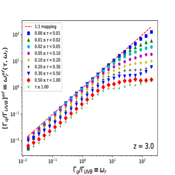
   Figure 11.— The plot shows the departure of the effective ionization correction parameter, $[\Gamma_{q}/\Gamma_{\textsc{uvb}}]^{ef}(\equiv\omega^{ef}_{r}(\tau,\omega_{r})$), from its theoretical value of $\Gamma_{q}/\Gamma_{\textsc{uvb}}(\equiv\omega_{r}$) in various pixel optical depth bins (listed in inset) obtained from spectra at low SDSS resolution ($R\sim$ 2000). Here, the $\omega_{r}$ is used to ionize the simulated IGM spectra as $\tau_{true}/[1+\omega_{r}]$. The $\tau_{true}$ and $\tau_{true}/[1+\omega_{r}]$ are convolved with Gaussian kernel corresponding to the SDSS resolution to obtain $\tau_{\textsc{igm}}$ and $\tau_{prox}$ respectively (e.g., see points shown in panel [5] of Fig. 10). The best fit is computed such that KS-test probability is maximum for $\tau_{prox}\times[1+\omega^{ef}_{r}(\tau,\omega_{r})]$ and $\tau_{\textsc{igm}}$ to belong to a similar distribution at each optical depth bin (binned in $\tau_{prox}$).

4. For the actual input ionization correction of [1+$\omega_{r}$], we consider the best fit value of output optimal ionization correction to be $[1+\omega^{ef}_{r}(\tau,\omega_{r})]$ in a given optical depth bin. For this, we use KS-test and compared the distribution of $\tau_{\textsc{igm}}$, with various distributions of $\tau_{prox}\times[1+\omega^{ef}_{r}(\tau,\omega_{r})]$, by varying the trial values of $\omega^{ef}_{r}(\tau)$ over a range of 1% to 200% of input $\omega_{r}$. The value of $[1+\omega^{ef}_{r}(\tau,\omega_{r})]$ resulting in maximal of $P_{null}$ by KS-test is selected as the best fit optimal value. We note that this optimized model value being for the mean value of the optical depth bin could also have an associated uncertainty. However, due to very small bin size of optical depth used here, this uncertainty is found to be negligible in comparison to the errors propagated to it based on the uncertainties in estimating the value of the pixel optical depth and its redshift as discussed in Sect. 3.2.2.

   The above procedure was repeated for various $\omega_{r}$ values ranging from 0.01 to 200 as shown in Fig. 11 for all the optical depth bins mentioned above. The plot is shown only for simulations at $z\sim 3.0$ as we found no significant evolution with the redshift. From this figure, it is evident that the required ionization correction departs towards a lower value compared to the theoretical equality line (shown as a red-dashed line in Fig. 11) with the increase in the pixel optical depth value. This is not surprising as higher optical depth pixels generally corresponds to the core of saturated lines where the optical depth reduction due to the ionization will be negligible. Therefore, the required ionization correction (to recover the unionized optical depth) will also be small. For instance, it can be noted from Fig. 11 that for a optical depth of $\sim$ 0.15 and for the typical range of 0.1-100 in $\omega_{r}$, the corresponding optimized $f(\omega_{r})$ varies over a small range of 0.1-5. This clearly demonstrates the need for optimizing the ionization correction (which is dependent on the pixel optical depth) for the analysis of the pixel optical depth based on the low-resolution spectrum (as in our case).

3.2.2 Pixel optical depth analysis using appropriate ionization correction

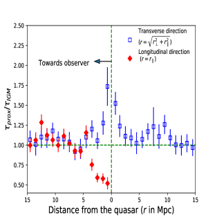
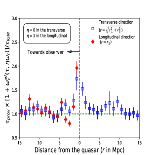
Figure 12.— Left panel: Ratio of the median optical depth value (within 1 Mpc bin) of proximity region ($\tau_{prox}$) to its median value in IGM ($\tau_{\textsc{igm}}$), showing a clear discrepancy at small radius between the measurements along the longitudinal (red, diamond) and the transverse (blue, square) directions. The resultant error bars consist of all the possible sources of errors such as flux error from photon counting statistics, error due to continuum placement uncertainties, r.m.s statistical error, sightline-to-sightline variance and emission redshift measurement error within the 1 Mpc radial distance bin as also used in Fig. 7 (e.g., Sect. 3.1.2). Right panel: Same as left panel but with optical depth scaled by [$1+\omega^{ef}_{r}(\tau,\omega_{r})$] for pixels belonging to the longitudinal proximity region (i.e., $median(\tau_{prox}\times[1+\omega^{ef}_{r}(\tau,\omega_{r})])/median[\tau_{\textsc{igm}}$]). Additionally, we also considered here the uncertainty in the scaled optical depth due to the uncertainties in estimating $\omega^{ef}_{r}(\tau,\omega_{r})$ (e.g., see Sect. 3.2.1).

In the left panel of Fig. 12, we plot the ratio of the median value of the optical depth in the proximity region to that of the corresponding IGM, $median[\tau_{prox}]/median[\tau_{\textsc{igm}}]$, at various radial distance bins of size 1 Mpc. The plot echoes the results based on the transmitted flux analysis (e.g., see Fig. 6) revealing a clear discrepancy at $r\leq 4$ Mpc, between the measurements along the longitudinal and transverse directions. We may recall that the shown error bars consist of all the possible sources of errors such as flux error from photon counting statistics, error due to continuum placement uncertainties, emission redshift measurement error, sightline-to-sightline variance and r.m.s statistical error within 1 Mpc radial distance bin as also used in Fig. 6 (e.g., Sect. 3.1.2). In this comparison, we have excluded the radial distances below 0.4 Mpc due to the lack of sufficient pixels within such separations along the transverse direction, where, a quasar pair can only contribute for pixels with $r>r_{\perp}$.

Based on the observed luminosity in the longitudinal direction, we have estimated the ionization corrected $median[\tau_{prox}]/median[\tau_{\textsc{igm}}]$ (refer to as an “average excess overdensity profile”), which is shown in the right panel of Fig. 12 (red, diamond). For this, we consider a pixel with the measured optical depth value $\tau_{i}$ at an absorption redshift of $z^{i}_{a}$. Firstly, based on the $\tau_{i}$ value, we choose the corresponding $\omega_{r}$ versus $\omega^{ef}_{r}(\tau,\omega_{r})$ curve from those shown in Fig. 11. Then the redshift difference between the pixel and the quasar allows us to compute the $\omega_{r}^{i}$ (using the measured luminosity e.g., see Eq. 14). We then estimate $\omega^{ef}_{r}(\tau,\omega_{r}^{i})$ using the cubic spline interpolation of the $\omega_{r}$ versus $\omega^{ef}_{r}(\tau,\omega_{r})$ curve (i.e., from Fig. 11). This optimal ionization correction (e.g., see Eq. 20) allows us to estimate the ionization corrected optical depth as $\tau_{off}\equiv\tau_{prox}\times[1+\omega^{ef}_{r}(\tau,\omega_{r})]$ (also referred to as scaled optical depth). Here, the error bar for the $\tau_{off}$ from the $\tau_{prox}$ are also propagated appropriately.

Additionally, we also considered the possible uncertainty in the $\tau_{off}$ due to $\omega^{ef}_{r}(\tau,\omega_{r})$ uncertainty. This error is (i) due to the uncertainty in the pixel optical depth ($\Delta\tau$) because of the strong dependence of $\omega^{ef}_{r}(\tau,\omega_{r})$ on the optical depth value and (ii) due to the uncertainty in $\omega_{r}$ propagated from the uncertainty in emission redshift measurements (reflected as $\Delta r$ uncertainty in the distance calculation). The former is estimated as;

$$|\omega^{ef}_{r}(\tau+\Delta\tau)-\omega^{ef}_{r}(\tau-\Delta\tau)|/2$$ (25)

while the latter as;

$$|\omega^{ef}_{r+\Delta r}(\tau)-\omega^{ef}_{r-\Delta r}(\tau)|/2.$$ (26)

Finally, both these uncertainties are added quadratically with the existing error estimates on the scaled optical depth of each pixel to get its final uncertainty.

This procedure of calculating the ionization correction is repeated for all pixels in the longitudinal direction. This has allowed us to plot the photoionization corrected excess overdensity profile along the longitudinal direction as shown in the right panel of Fig. 12 (shown by red, diamond). The trend in this figure suggests the existence of an “excess overdensity” at $r\leq 5$ Mpc of the quasar. We note that the impact of peculiar velocities might be significant in these radial bins which may make our distance estimation uncertain. However, given the similarity of this “excess overdensity” with that of the transverse direction for which the quasar’s ionization correction is not applied, shows that the quasar’s illumination in the transverse direction has to be smaller in comparison to the illumination measured in the longitudinal direction (estimated based on measured luminosity in the longitudinal direction). Therefore, for the ionization correction in the transverse direction, we have followed the above procedure by replacing $\omega_{r}^{i}$ with $\eta\omega_{r}^{i}$, for an allowed range of $\eta$ from zero to unity. For computing the best fit value of $\eta$, we have used $\chi^{2}$ analysis over 0-15 Mpc radial distance bins to statistically match the distribution of $\tau_{prox}\times[1+\omega^{ef}_{r}(\tau,\omega_{r})]/\tau_{\textsc{igm}}$ in the longitudinal direction with various distributions of $[1+\omega^{ef}_{r}(\tau,\eta\omega_{r})]/\tau_{\textsc{igm}}$ in the transverse direction by varying the trial values of $\eta$ from zero to unity in steps of 0.025. Here, we limit this comparison only to the pixels with $z_{a}<z_{f}$ (i.e., only among regions towards the observer). This results in a $\chi^{2}$ versus $\eta$ curve as shown in Fig. 13. As evident from this plot, the minimum value of $\chi^{2}$ is found for $\eta=0$ with $\chi_{min}^{2}=14.76$. The value of $\chi^{2}_{min}+n^{2}$ in this $\chi^{2}$ versus $\eta$ curve is used to estimate the $n\sigma$ confidence in the $\eta$ value (assuming the Gaussian nature of the errors) using cubic spline interpolation. This results in $\eta\leq 0.03,0.16$ and $0.27$ at 1$\sigma$, 2$\sigma$ and 3$\sigma$ level respectively. This suggests that the quasar’s average illumination in our sample on the H i cloud in the transverse direction is less than 27% (at 3$\sigma$ confidence level) of that measured along the longitudinal direction. The above 3$\sigma$ limit changes from the 27% value to 31% if we exclude the first radial bin (i.e., 0-1 Mpc) from our above analysis, in view of the possible significant impact of the peculiar velocities close to the quasars.

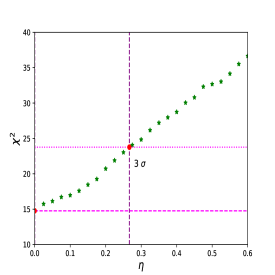
Figure 13.— The plot shows the $\chi^{2}$ values calculated between $\tau_{prox}\times[1+\omega^{ef}_{r}(\tau,\omega_{r})]/\tau_{\textsc{igm}}$ of LPE and $\tau_{prox}\times[1+\omega^{ef}_{r}(\tau,\eta\omega_{r})]/\tau_{\textsc{igm}}$ of TPE, where $\eta$ is the fraction of the illumination in the transverse direction as compared to the longitudinal direction, ranging in $0\leq\eta\leq 1$ (see text). The horizontal dotted line gives the $\chi^{2}$ that corresponds to 3$\sigma$ range of $\eta$ around the best fit value.

3.2.3 Impact of Ly continuum uncertainty based on spectral index variation

As discussed in Sect. 2.3, we have adopted a simplistic treatment of the quasar SED, by using a simple power-law continuum composite of AGN spectrum (e.g., see Eq. 6) with no scatter in this relation. Any scatter around this spectral slope will, in fact, affect the ionization scaling, being it inversely proportional to the spectral slope of the quasar (e.g., see Eq. 18). Therefore, in order see the effect of spectral slope uncertainty on the inferred overdensity, we have repeated our LPE analysis using two extreme values of the spectral slope viz., $\alpha_{uv}=$ 0.56 and 1.96, based on the range given by Khaire (2017), assuming $\Gamma_{\textsc{uvb}}$ to be unchanged. We have re-calculated the overdensity profile along the longitudinal direction using these two extreme values, as shown in Fig. 14. As can be seen from this figure that the profile of overdensity is similar for these two extreme values of the spectral slope as is found using the optimal value of $\alpha_{uv}=1.57$ (except the change in amplitude). In addition to this, their corresponding difference in the amplitude of overdensity (i.e., higher for smaller $\alpha_{uv}$ value) is also consistent within 1$\sigma$, except in lower radial distance bin (approaching up to 2$\sigma$) as expected due to the $r^{-2}\times\alpha^{-1}$ dependency of $\Gamma_{q}$ (e.g., see Eq. 18). Moreover, we also notice that the actual deviation, based on the use of an individual $\alpha_{uv}$ value of the quasars will be smaller than that estimated here based on these two extreme values. As a result, we can conclude that any uncertainty due to the use of constant $\alpha_{uv}$ value for all our foreground quasars will not have any significant impact on our results. However, this will add a small scatter to the derived density profile.

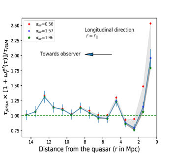
Figure 14.— The plot shows the variation of excess overdensity in the longitudinal direction by taking two possible extreme values of the spectral index while correcting for the ionization by the foreground quasars.

4. Discussions

Our detailed analysis of the proximity effect based on the transmitted flux measured from closely spaced quasar pairs, detected in the SDSS, shows a clear difference in the transmitted flux profile along the longitudinal and the transverse directions, having more H i absorption in the latter case (e.g., see Fig. 6). This is also reflected in our pixel optical depth analysis (e.g., see Fig. 8). After applying appropriate ionization corrections in the longitudinal direction, we have derived ionization corrected average excess density profile which shows excess up to $r\leq 5$ Mpc. Surprisingly, it matches with the uncorrected average excess overdensity profile in the transverse direction (e.g., see Fig. 12). This led to an important result that the H i absorbing clouds in the transverse direction on an average receive the quasar’s illumination $\leq$27% (at 3$\sigma$ confidence level) as compared to that along the longitudinal direction (e.g., see Fig. 13). Below, we discuss our results, in the context of excess overdensity as well as anisotropy in the ionizing radiation field.

4.1. Overdensity

It can be noted from the right panel of the Fig. 12 that our analysis shows an excess overdensity up to $r\leq 5$ Mpc with an increasing amplitude towards the foreground quasar. The evidence of overdensity inferred in our analysis is also found to be consistent with many previous such studies (D’Odorico et al., 2002; Rollinde et al., 2005; Guimarães et al., 2007; Prochaska et al., 2013; Adams et al., 2015). However, we note that the extent of the overdensity around the quasars found in our analysis is smaller than those found using LPE by Rollinde et al. (2005) and Guimarães et al. (2007), though the magnitude of overdensity is quite similar at smaller distances. One of the reasons for this difference could be that the quasars used in their sample are systematically brighter than the quasars used in our sample. Also, these studies use quasar’s spectra with better spectral resolution and SNR. This was affordable in these studies, as their main aim was only to probe the longitudinal proximity region for which any high-quality spectrum can be included without satisfying an additional requirement of being a member of closely separated quasar pair as needed for the TPE analysis.

We constrain the overdensity profile along the longitudinal direction using the quasar luminosity and optimal ionization correction obtained using our simulations. This can in principle be used to place constraints on the mass of the host galaxies. However, a more precise constraint can also be achieved by the longitudinal proximity analysis based on a larger sample (affordable due to the absence of an additional requirement of closely separated quasar pairs) and realistic simulations that also models quasars along with their ionization influence. The coarse sampling of 1 Mpc achieved in our analysis based on these 181 quasars pairs, may not be enough to resolve the mass information which is mostly confined to $r\leq$1 Mpc (e.g., see Faucher-Giguère et al., 2008a). Additionally, the ionization correction in 0-1 Mpc bin might also be highly uncertain due to the possible impact of peculiar velocities close to the quasar. Therefore, in what follows, we basically focus on the ionization anisotropy.

4.2. Anisotropic distribution of radiation?

The difference in the transmitted flux and the optical depth found between the longitudinal and the transverse direction, is also found consistent with the studies of Prochaska et al. (2013) and Kirkman & Tytler (2008), though based on a slightly different analysis. A few noticeable differences are that Prochaska et al. (2013) have used a control sample for the study of TPE and reported the anisotropy by comparing with a previous study of LPE which is inferred from a different quasar sample. However, Kirkman & Tytler (2008) studied both the LPE and TPE using the same set of the foreground quasars (similar to our analysis), but instead of using a control sample they have carried out the analysis correcting the observed optical depth for the redshift evolution.

The inferred anisotropy in the transmitted flux and the optical depth can have many physical interpretations, such as, either an intrinsic anisotropy of the emitted radiation or due to asymmetric obscuration by a “dusty torus” in the context of standard AGN-unification scheme (e.g., see Antonucci, 1993; Elvis, 2000). The latter scenario seems to be more likely as there have been a number of observational evidence which directly detects the presence of an obscuring torus surrounding a central continuum source (e.g., see Davies et al., 2015; Almeyda et al., 2017). This will result in the obscuration of the ionizing photons in the direction of the equatorial plane of the torus. However, such an interpretation will be ruled out if the quasar sample used in our analysis have random orientations relative to our line-of-sight.

On the other hand, in any flux-limited survey, the quasars would be preferentially observed along the direction in which they appear to be brighter such as in the direction perpendicular to the plane of the dusty torus. This could be a likely scenario, as for the majority of SDSS DR12 quasars the redshift measurements are derived from “broad emission lines” (e.g., see Alexandroff et al., 2013; Pâris et al., 2017) which are prominent in the quasars having their torus perpendicular to our line-of-sight, commonly known as Type-I AGNs (in the standard AGN-unification scheme). Therefore, we checked the velocity width (FWHM) of the C iv line as provided by SDSS (e.g., see Pâris et al., 2017). Out of 181 foreground quasars in our sample, it was available for 175 of them (6 of them did not have prominent C iv emission line) and indeed all of them have FWHM $>2000$ km s^-1. This suggests that our sample is dominated by Type-I AGNs. It will also be interesting to extend our analysis (based on Type-I AGNs as foreground quasars) by using the Type-II AGNs as foreground quasars, in-spite of the scarcity of observed Type-II AGNs at higher redshifts (see also, Lu & Yu, 2011). This will confirm the scenario of anisotropic obscuration, if one finds an exactly opposite trend as compared to our above analysis, due to the presence of dusty torus along the longitudinal direction in Type-II AGNs.

An alternative possibility for the observed anisotropy among the longitudinal and the transverse directions could be the finite lifetime of the quasar. As discussed in Sect. 1 that the light from the foreground quasars has to travel an extra path in the transverse direction (i.e., $r_{\perp}$/c). Therefore, due to quasar’s finite lifetime, its radiation might not be apparent along the background quasar when we see the foreground quasar in its initial stages of the active phase. We use the median $r_{\perp}$/c of our sample i.e., 0.5 Mpc, which results in an extra light travel time of 0.5 Mpc/c $\sim$ 1.6 Myr. In addition to this, the fact that we observe the overdensity even in the first radial bin of the transverse direction implies that the quasar was not ionizing before 1.6 Myr ago i.e., quasar lifetime $t_{Q}\leq 1.6$ Myr.

Moreover, the estimate of quasar’s lifetime reported in literature, based on various techniques, varies over a wide range from 10⁴ yrs to 10⁷ yrs (e.g., see Srianand, 1997; Gonçalves et al., 2008; Trainor & Steidel, 2013; Borisova et al., 2016; Oppenheimer et al., 2017). For instance, Bajtlik et al. (1988) estimated the quasar’s lifetime to be around 10⁴ yrs using the equilibration time-scale $\sim\Gamma_{\textsc{H~{}{\sc i}}}^{-1}$ (see also, Carswell et al., 1982; Dall’Aglio et al., 2008b; Eilers et al., 2017, 2018). However, based on the quasar variability, Schawinski et al. (2015) estimated the typical value to be 0.1 Myr (see also, Schawinski et al., 2010). On the other extreme, Schmidt et al. (2018) have used longitudinal He ii proximity effect and estimated quasar’s lifetime to be $\sim$30 Myr (see also, Hogan et al., 1997; Anderson et al., 1999; Zheng et al., 2015; Khrykin et al., 2016; Schmidt et al., 2017). Given the wide range of inferred values of quasar’s lifetime it is difficult to draw any conclusion on the value of 1.6 Myr as we have estimated above.

Another possible scenario could be the inflow of matter onto the quasar massive halo (see also, Faucher-Giguère et al., 2008a). This could also introduce anisotropic effects on the measured redshift of the absorbing clouds. For instance, due to the inflow, the redshift distortion will be more in the longitudinal direction as compared to the transverse direction, with the latter being affected by only the projected velocity component of the inflow. As pointed out by Faucher-Giguère et al. (2008a), it will amount to a typical underestimation of the distance by 1 Mpc in the longitudinal direction which is too small to explain the significant difference we noticed among these two directions over a range up to 4 Mpc. Moreover, this implies that we might have applied an ionization correction a bit more than the actual value in the longitudinal direction (due to the distance underestimation) to scale up the observed optical depth (compared to the true ionization correction). However, in view of the fact that the scaled optical depth in the longitudinal direction does not exceed even the value of unscaled optical depth (i.e., without ionization correction) in the transverse direction, we conclude that any possible impact of an inflow will be negligible to the measured anisotropy. Similar to inflows, quasars also do have outflows, which will have an impact on redshift distortion opposite to that of the inflow scenario. However, given the large difference between the longitudinal and transverse directions, it seems that simply the effect of inflow and/or outflow cannot explain the above observed discrepancy inferred in the quasar’s illumination among these two directions.

The most probable scenario for the observed anisotropy (among the longitudinal and transverse directions) seems to be anisotropic obscuration of the ionizing radiation, probably due to the presence of the dusty torus. This also has an important implication for the AGN unification scheme. For instance, Schirber et al. (2004) used the absence of TPE to constrain such dusty torus to have an opening angle of $\sim$20$\degree$, and Kirkman & Tytler (2008) over a range of 60$\degree$ to 120$\degree$ (also confirmed by Lu & Yu, 2011). We have constrained the average quasar’s illumination “in the framework of the shadowing by the torus” on the H i cloud in the transverse direction in comparison to the longitudinal direction to be less than 27% at 3$\sigma$ confidence (see Sect. 3.2.2 for details).

Furthermore, we also note that a comparison of the transverse proximity effect, towards the observer and towards the background quasars can allow us to probe the temporal evolution of the quasar’s ionization (assuming on an average the matter distribution is spherically symmetric). For instance, Kirkman & Tytler (2008) found an asymmetry with more absorption toward background quasars and use it to constrain the episodic lifetime of the quasars to be $\sim$ 1 Myr. In our study, we do not find such a difference as can be seen from Fig. 6. Here, we may also recall that in our analysis, the emission redshifts are corrected for the systematic redshift by 229 km s^-1. The shift of the peak optical depth position with respect to the systematic redshift of the quasar is close to the average systematic redshift uncertainty provided by Shen et al. (2016) for the SDSS quasars. This once again reiterate the importance of accurately measuring the systematic redshift of the quasars. The absence of such systematic correction in the emission redshift would have introduced any fiducial asymmetry (e.g., see Fig. 7) and hence may lead to an erroneous interpretation in constraining the episodic quasar lifetime.

5. Summary and Conclusions

The proximity effect is a very powerful tool to probe the environment of the quasars as well as to measure the intensity of the diffuse UVB radiation. Many of the past studies for the proximity effect have found significantly higher H i absorption near the quasar as compared to the expected value based on the statistics of faraway IGM (Croft, 2004; Schirber et al., 2004; Rollinde et al., 2005; Guimarães et al., 2007; Kirkman & Tytler, 2008; Prochaska et al., 2013; Finley et al., 2014; Adams et al., 2015). In addition, Prochaska et al. (2013) and Kirkman & Tytler (2008) have also reported discrepancy in the H i absorption along the longitudinal and the transverse directions in their sample of quasar pairs. The absorption was found to be stronger in the transverse direction. To probe the environment of the quasars at even smaller scales, both in the longitudinal and the transverse directions, we have used a sample of 181 projected quasar pairs from SDSS DR12 having a small angular separation of $<1.5$ arcmin (e.g., see Fig. 1).

Our sample of quasar pairs is compiled using proper selection criteria on the redshift range and angular sky separation. We also removed special cases such as: (i) BAL quasars, (ii) sightlines which have associated absorbers, LLS, DLAs or sub-DLAs in the proximity region (e.g., see Sect. 2.1) and (iii) pairs having velocity separation $<2000$ km s^-1 etcetera (e.g., see Sect. 2.2).

This well selected quasar sample is analyzed with noticeable improvements such as:

1. In order to compare the distribution of the optical depth and the transmitted flux measured in the proximity region both along the longitudinal and the transverse directions, we have used the same set of foreground quasars.

2. For comparison with the IGM, we have used the redshift and SNR matched control sample, instead of using the redshift scaling to take into account the redshift evolutions of the IGM optical depth as used in many previous such studies (e.g., Sect. 2.4, Fig. 2).

3. We have considered all the possible sources of errors in the flux and optical depth analysis such as (i) error contributed by the continuum fitting uncertainty using mock spectra for each sightline in our sample (e.g., see Sect. 3.1.1 and Figs. 3, 4, 5), (ii) the error due to photon counting statistics, (iii) sightline-to-sightline variance, (iv) emission redshift measurement error and (v) the r.m.s statistical error within the 1 Mpc radial distance bin (e.g., Sect. 3.1.2).

4. The observed optical depth in the proximity region can be enhanced due to the excess overdensity in which the quasar resides as well as be reduced by the excess quasar ionization. To lift this degeneracy between the quasar’s ionization and overdensity, we use the precise UVB radiation measurements from Khaire & Srianand (2015a) in conjunction with the known quasar luminosity in the longitudinal direction. However, the analytical [$1+\omega_{r}$] ionization correction (i.e., Eq. 14-20) for low/moderate resolution and low SNR is not found to be appropriate (e.g., see Sect. 3.2). Therefore, we have used detailed hydrodynamical simulation to validate ionization correction (i.e., $[1+\omega^{ef}_{r}(\tau,\omega_{r})]$) optimal for low/moderate resolution spectra (e.g., see Sect. 3.2.1 and Figs. 10, 11).

Our detailed analysis of the transmitted flux and the pixel optical depth, both in the longitudinal and the transverse directions, led us to the following main conclusions:

1. In the longitudinal direction, the proximity region within 4 Mpc (proper distance) shows an enhancement of the transmitted flux in comparison to its control sample (e.g., see Sect. 3.1.3, Fig. 6), while the trend is found to be reversed in the transverse direction ($r\leq 2$ Mpc). This suggests the dominance of the quasars ionization in the longitudinal direction whereas higher H i absorption in the transverse direction. A corresponding consistent trend is also seen in the CPDFs of the effective optical depth in different radial distance bins from the foreground quasar (e.g., see Sect. 3.1.4, Fig. 8).

2. The average absorption profile we measured in the transverse direction is found to be symmetric with respect to the quasar systematic redshift (e.g., see Figs. 6, 7). We also show the actual profile is sensitive to the assumed quasar redshifts. Therefore, to make an important progress in mapping the density profile, NIR spectra based systematic redshift measurements are imperative.

3. We estimated the quasar’s ionization based on the measured luminosity in the longitudinal direction to get the ionization corrected pixel optical depth distribution. This enabled us to estimate the average excess overdensity profile (after ionization correction), which is found to be decreasing radially outward from the quasars and with an excess up to $r\leq 5$ Mpc.

4. Unlike the longitudinal direction, due to the lack of direct measurement of the quasar’s luminosity in the transverse direction, the direct estimation of its average excess overdensity profile (after ionization correction) was not feasible. However, it is reasonable to assume the overdensity distribution to be symmetric as we average over a large number of quasars. This in conjunction with the fact that we observed more H i absorption in the transverse direction clearly suggests that the quasar’s obscuration in our sample is more in the transverse direction. This has allowed us to constrain the quasar’s illumination on H i absorbing cloud in the transverse direction to be $\leq$27% (3$\sigma$ confidence level) of that along the longitudinal direction (e.g., see Fig. 13). The above scenario of anisotropic obscuration after excluding many other possibilities (e.g., see Sect. 4.2) is also found consistent with the fact that all of our foreground quasars happen to be Type-I AGNs (based on the velocity width of C iv emission line) for which dusty torus will be mainly in the transverse direction. This also independently confirms the presence of a dusty torus in the AGNs, which is a key feature of the AGN unification scheme.

For further improvement, it will also be interesting to extend our analysis (based on Type-I AGN as foreground quasars) by using the Type-II AGN as well, beside enlarging the sample size of such quasar pairs at separation $<1$ arcmin (as also suggested by Lu & Yu, 2011) The improvement in the sample size will require a dedicated program of long-slit spectroscopy with 3-4 m class telescopes by orienting the slit to cover both members of a probable quasar pair even at separation $<$ 1 arcmin which might have been missed by SDSS observations due to fibre collision problem; so as to probe the quasar lifetime, anisotropic obscuration and their environment even at kpc scales.

References

- Adams et al. (2015) Adams, S. M., Martini, P., Croxall, K. V., Overzier, R. A., & Silverman, J. D. 2015, MNRAS, 448, 1335
- Adelberger (2004) Adelberger, K. L. 2004, ApJ, 612, 706
- Alexandroff et al. (2013) Alexandroff, R., Strauss, M. A., Greene, J. E., et al. 2013, MNRAS, 435, 3306
- Almeyda et al. (2017) Almeyda, T., Robinson, A., Richmond, M., Vazquez, B., & Nikutta, R. 2017, ApJ, 843, 3
- Anderson et al. (1999) Anderson, S. F., Hogan, C. J., Williams, B. F., & Carswell, R. F. 1999, The Astronomical Journal, 117, 56
- Antonucci (1993) Antonucci, R. 1993, ARA&A, 31, 473
- Bahcall et al. (1969) Bahcall, J. N., Schmidt, M., & Gunn, J. E. 1969, ApJ, 157, L77
- Bahcall & Chokshi (1991) Bahcall, N. A., & Chokshi, A. 1991, ApJ, 380, L9
- Bajtlik et al. (1988) Bajtlik, S., Duncan, R. C., & Ostriker, J. P. 1988, ApJ, 327, 570
- Bautista et al. (2015) Bautista, J. E., Bailey, S., Font-Ribera, A., et al. 2015, jcap, 5, 060
- Bechtold (1994) Bechtold, J. 1994, ApJS, 91, 1
- Bennett et al. (2014) Bennett, C. L., Larson, D., Weiland, J. L., & Hinshaw, G. 2014, ApJ, 794, 135
- Bergeron & Ikeuchi (1990) Bergeron, J., & Ikeuchi, S. 1990, A&A, 235, 8
- Bi (1993) Bi, H. 1993, ApJ, 405, 479
- Bi & Davidsen (1997) Bi, H., & Davidsen, A. F. 1997, ApJ, 479, 523
- Bolton et al. (2012) Bolton, A. S., Schlegel, D. J., Aubourg, É., et al. 2012, AJ, 144, 144
- Bolton et al. (2006) Bolton, J. S., Haehnelt, M. G., Viel, M., & Carswell, R. F. 2006, MNRAS, 366, 1378
- Bolton et al. (2017) Bolton, J. S., Puchwein, E., Sijacki, D., et al. 2017, MNRAS, 464, 897
- Borde et al. (2014) Borde, A., Palanque-Delabrouille, N., Rossi, G., et al. 2014, jcap, 7, 005
- Borisova et al. (2016) Borisova, E., Lilly, S. J., Cantalupo, S., et al. 2016, The Astrophysical Journal, 830, 120
- Bowen et al. (2006) Bowen, D. V., Hennawi, J. F., Ménard, B., et al. 2006, ApJ, 645, L105
- Busca et al. (2013) Busca, N. G., Delubac, T., Rich, J., et al. 2013, A&A, 552, A96
- Calverley et al. (2011) Calverley, A. P., Becker, G. D., Haehnelt, M. G., & Bolton, J. S. 2011, MNRAS, 412, 2543
- Carswell et al. (1982) Carswell, R. F., Whelan, J. A. J., Smith, M. G., Boksenberg, A., & Tytler, D. 1982, MNRAS, 198, 91
- Cen et al. (1994) Cen, R., Miralda-Escudé, J., Ostriker, J. P., & Rauch, M. 1994, ApJ, 437, L9
- Choudhury et al. (2001a) Choudhury, T. R., Padmanabhan, T., & Srianand, R. 2001a, MNRAS, 322, 561
- Choudhury et al. (2001b) Choudhury, T. R., Srianand, R., & Padmanabhan, T. 2001b, ApJ, 559, 29
- Cocke & Tifft (1989) Cocke, W. J., & Tifft, W. G. 1989, ApJ, 346, 613
- Cooke et al. (1997) Cooke, A. J., Espey, B., & Carswell, R. F. 1997, MNRAS, 284, 552
- Cristiani et al. (1995) Cristiani, S., D’Odorico, S., Fontana, A., Giallongo, E., & Savaglio, S. 1995, MNRAS, 273, 1016
- Croft (2004) Croft, R. A. C. 2004, ApJ, 610, 642
- Croft et al. (2002) Croft, R. A. C., Hernquist, L., Springel, V., Westover, M., & White, M. 2002, ApJ, 580, 634
- Croft et al. (1998) Croft, R. A. C., Weinberg, D. H., Katz, N., & Hernquist, L. 1998, ApJ, 495, 44
- Croom et al. (2005) Croom, S. M., Boyle, B. J., Shanks, T., et al. 2005, MNRAS, 356, 415
- Dall’Aglio & Gnedin (2010) Dall’Aglio, A., & Gnedin, N. Y. 2010, ApJ, 722, 699
- Dall’Aglio et al. (2008a) Dall’Aglio, A., Wisotzki, L., & Worseck, G. 2008a, A&A, 491, 465
- Dall’Aglio et al. (2008b) —. 2008b, A&A, 480, 359
- Davé et al. (2010) Davé, R., Oppenheimer, B. D., Katz, N., Kollmeier, J. A., & Weinberg, D. H. 2010, MNRAS, 408, 2051
- Davies et al. (2015) Davies, R. I., Burtscher, L., Rosario, D., et al. 2015, ApJ, 806, 127
- Delubac et al. (2015) Delubac, T., Bautista, J. E., Busca, N. G., et al. 2015, A&A, 574, A59
- D’Odorico et al. (2002) D’Odorico, V., Petitjean, P., & Cristiani, S. 2002, A&A, 390, 13
- Efron & J. Tibshirani (1993) Efron, B., & J. Tibshirani, R. 1993, An Introduction To The Bootstrap
- Efstathiou et al. (2000) Efstathiou, G., Schaye, J., & Theuns, T. 2000, in Philosophical Transactions of the Royal Society of London Series A, Vol. 358, Astronomy, physics and chemistry of H+3, 2049
- Eftekharzadeh et al. (2017) Eftekharzadeh, S., Myers, A. D., Hennawi, J. F., et al. 2017, MNRAS, 468, 77
- Eilers et al. (2017) Eilers, A.-C., Davies, F. B., Hennawi, J. F., et al. 2017, The Astrophysical Journal, 840, 24
- Eilers et al. (2018) Eilers, A.-C., Hennawi, J. F., & Davies, F. B. 2018, The Astrophysical Journal, 867, 30
- Elvis (2000) Elvis, M. 2000, ApJ, 545, 63
- Farina et al. (2013) Farina, E. P., Falomo, R., Decarli, R., Treves, A., & Kotilainen, J. K. 2013, MNRAS, 429, 1267
- Faucher-Giguère et al. (2008a) Faucher-Giguère, C.-A., Lidz, A., Zaldarriaga, M., & Hernquist, L. 2008a, ApJ, 673, 39
- Faucher-Giguère et al. (2008b) Faucher-Giguère, C.-A., Prochaska, J. X., Lidz, A., Hernquist, L., & Zaldarriaga, M. 2008b, ApJ, 681, 831
- Fechner & Reimers (2007) Fechner, C., & Reimers, D. 2007, A&A, 463, 69
- Finley et al. (2014) Finley, H., Petitjean, P., Noterdaeme, P., & Pâris, I. 2014, A&A, 572, A31
- Fisher et al. (1996) Fisher, K. B., Bahcall, J. N., Kirhakos, S., & Schneider, D. P. 1996, ApJ, 468, 469
- Font-Ribera et al. (2013) Font-Ribera, A., Arnau, E., Miralda-Escudé, J., et al. 2013, Journal of Cosmology and Astroparticle Physics, 2013, 018
- Fukugita et al. (2004) Fukugita, M., Nakamura, O., Schneider, D. P., Doi, M., & Kashikawa, N. 2004, ApJ, 603, L65
- Gaikwad et al. (2018) Gaikwad, P., Choudhury, T. R., Srianand, R., & Khaire, V. 2018, MNRAS, 474, 2233
- Gallerani (2011) Gallerani, S. 2011, in Journal of Physics Conference Series, Vol. 280, Journal of Physics Conference Series, 012008
- Giallongo et al. (1996) Giallongo, E., Cristiani, S., D’Odorico, S., Fontana, A., & Savaglio, S. 1996, ApJ, 466, 46
- Gonçalves et al. (2008) Gonçalves, T. S., Steidel, C. C., & Pettini, M. 2008, ApJ, 676, 816
- Guimarães et al. (2007) Guimarães, R., Petitjean, P., Rollinde, E., et al. 2007, MNRAS, 377, 657
- Gunn & Peterson (1965) Gunn, J. E., & Peterson, B. A. 1965, ApJ, 142, 1633
- Haardt & Madau (2012) Haardt, F., & Madau, P. 2012, ApJ, 746, 125
- Hartwick & Schade (1990) Hartwick, F. D. A., & Schade, D. 1990, ARA&A, 28, 437
- Hennawi & Prochaska (2007) Hennawi, J. F., & Prochaska, J. X. 2007, ApJ, 655, 735
- Hennawi & Prochaska (2013) —. 2013, ApJ, 766, 58
- Hennawi et al. (2006) Hennawi, J. F., Prochaska, J. X., Burles, S., et al. 2006, ApJ, 651, 61
- Hernquist et al. (1996) Hernquist, L., Katz, N., Weinberg, D. H., & Miralda-Escudé, J. 1996, ApJ, 457, L51
- Hewett & Wild (2010) Hewett, P. C., & Wild, V. 2010, MNRAS, 405, 2302
- Hogan et al. (1997) Hogan, C. J., Anderson, S. F., & Rugers, M. H. 1997, AJ, 113, 1495
- Hogg (1999) Hogg, D. W. 1999, ArXiv Astrophysics e-prints, astro-ph/9905116
- Hopwood et al. (2010) Hopwood, R., Serjeant, S., Negrello, M., et al. 2010, ApJ, 716, L45
- Hui et al. (1997a) Hui, L., Gnedin, N. Y., & Zhang, Y. 1997a, arXiv:astro-ph/9702167v1, astro-ph/9702167
- Hui et al. (1997b) —. 1997b, ApJ, 486, 599
- Hui & Rutledge (1999) Hui, L., & Rutledge, R. E. 1999, ApJ, 517, 541
- Khaire (2017) Khaire, V. 2017, MNRAS, 471, 255
- Khaire & Srianand (2015a) Khaire, V., & Srianand, R. 2015a, MNRAS, 451, L30
- Khaire & Srianand (2015b) —. 2015b, ApJ, 805, 33
- Khaire & Srianand (2019) —. 2019, MNRAS, 484, 4174
- Khrykin et al. (2016) Khrykin, I. S., Hennawi, J. F., McQuinn, M., & Worseck, G. 2016, ApJ, 824, 133
- Kim et al. (2002) Kim, T.-S., Carswell, R. F., Cristiani, S., D’Odorico, S., & Giallongo, E. 2002, MNRAS, 335, 555
- Kim & Croft (2008) Kim, Y.-R., & Croft, R. A. C. 2008, MNRAS, 387, 377
- Kirkman & Tytler (2008) Kirkman, D., & Tytler, D. 2008, MNRAS, 391, 1457
- Kulkarni & Fall (1993) Kulkarni, V. P., & Fall, S. M. 1993, ApJ, 413, L63
- Lau et al. (2016) Lau, M. W., Prochaska, J. X., & Hennawi, J. F. 2016, ApJS, 226, 25
- Lau et al. (2018) —. 2018, ApJ, 857, 126
- Lee et al. (2012) Lee, K.-G., Suzuki, N., & Spergel, D. N. 2012, AJ, 143, 51
- Lehner et al. (2007) Lehner, N., Savage, B. D., Richter, P., et al. 2007, ApJ, 658, 680
- Liske & Williger (2001) Liske, J., & Williger, G. M. 2001, MNRAS, 328, 653
- Loeb & Eisenstein (1995) Loeb, A., & Eisenstein, D. J. 1995, ApJ, 448, 17
- Lu et al. (1991) Lu, L., Wolfe, A. M., & Turnshek, D. A. 1991, ApJ, 367, 19
- Lu & Yu (2011) Lu, Y., & Yu, Q. 2011, ApJ, 736, 49
- Machacek et al. (2000) Machacek, M. E., Bryan, G. L., Meiksin, A., et al. 2000, ApJ, 532, 118
- Madau & Pozzetti (2000) Madau, P., & Pozzetti, L. 2000, MNRAS, 312, L9
- McDonald et al. (2001) McDonald, P., Miralda-Escudé, J., Rauch, M., et al. 2001, ApJ, 562, 52
- Meiksin & White (2003) Meiksin, A., & White, M. 2003, MNRAS, 342, 1205
- Miralda-Escudé et al. (1996) Miralda-Escudé, J., Cen, R., Ostriker, J. P., & Rauch, M. 1996, ApJ, 471, 582
- Muecket et al. (1996) Muecket, J. P., Petitjean, P., Kates, R. E., & Riediger, R. 1996, A&A, 308, 17
- Murdoch et al. (1986) Murdoch, H. S., Hunstead, R. W., Pettini, M., & Blades, J. C. 1986, ApJ, 309, 19
- Noterdaeme et al. (2009) Noterdaeme, P., Petitjean, P., Ledoux, C., & Srianand, R. 2009, A&A, 505, 1087
- Noterdaeme et al. (2012) Noterdaeme, P., Petitjean, P., Carithers, W. C., et al. 2012, A&A, 547, L1
- Nusser & Haehnelt (1999) Nusser, A., & Haehnelt, M. 1999, MNRAS, 303, 179
- Oppenheimer et al. (2017) Oppenheimer, B. D., Segers, M., Schaye, J., Richings, A. J., & Crain, R. A. 2017, Monthly Notices of the Royal Astronomical Society, 474, 4740
- Osterbrock & Ferland (2006) Osterbrock, D. E., & Ferland, G. J. 2006, Astrophysics of gaseous nebulae and active galactic nuclei
- Ozbek et al. (2016) Ozbek, M., Croft, R. A. C., & Khandai, N. 2016, MNRAS, 456, 3610
- Pâris et al. (2017) Pâris, I., Petitjean, P., Ross, N. P., et al. 2017, A&A, 597, A79
- Partl et al. (2011) Partl, A. M., Müller, V., Yepes, G., & Gottlöber, S. 2011, MNRAS, 415, 3851
- Pichon et al. (2001) Pichon, C., Vergely, J. L., Rollinde, E., Colombi, S., & Petitjean, P. 2001, MNRAS, 326, 597
- Pieri et al. (2010) Pieri, M. M., Frank, S., Weinberg, D. H., Mathur, S., & York, D. G. 2010, ApJ, 724, L69
- Prochaska & Hennawi (2009) Prochaska, J. X., & Hennawi, J. F. 2009, ApJ, 690, 1558
- Prochaska et al. (2014) Prochaska, J. X., Lau, M. W., & Hennawi, J. F. 2014, ApJ, 796, 140
- Prochaska et al. (2013) Prochaska, J. X., Hennawi, J. F., Lee, K.-G., et al. 2013, ApJ, 776, 136
- Rauch (1998) Rauch, M. 1998, ARA&A, 36, 267
- Regan et al. (2007) Regan, J. A., Haehnelt, M. G., & Viel, M. 2007, MNRAS, 374, 196
- Rodríguez-Torres et al. (2017) Rodríguez-Torres, S. A., Comparat, J., Prada, F., et al. 2017, MNRAS, 468, 728
- Rollinde et al. (2001) Rollinde, E., Petitjean, P., & Pichon, C. 2001, A&A, 376, 28
- Rollinde et al. (2005) Rollinde, E., Srianand, R., Theuns, T., Petitjean, P., & Chand, H. 2005, MNRAS, 361, 1015
- Sargent (1980) Sargent, W. L. W. 1980, Phys. Scr, 21, 753
- Schawinski et al. (2015) Schawinski, K., Koss, M., Berney, S., & Sartori, L. F. 2015, MNRAS, 451, 2517
- Schawinski et al. (2010) Schawinski, K., Evans, D. A., Virani, S., et al. 2010, The Astrophysical Journal, 724, L30
- Schaye (2001a) Schaye, J. 2001a, arXiv:astro-ph/0112022, astro-ph/0112022
- Schaye (2001b) —. 2001b, ApJ, 559, 507
- Schirber et al. (2004) Schirber, M., Miralda-Escudé, J., & McDonald, P. 2004, ApJ, 610, 105
- Schmidt et al. (2018) Schmidt, T. M., Hennawi, J. F., Worseck, G., et al. 2018, ApJ, 861, 122
- Schmidt et al. (2017) Schmidt, T. M., Worseck, G., Hennawi, J. F., Prochaska, J. X., & Crighton, N. H. M. 2017, The Astrophysical Journal, 847, 81
- Scott et al. (2000) Scott, J., Bechtold, J., Dobrzycki, A., & Kulkarni, V. P. 2000, ApJS, 130, 67
- Seljak et al. (2003) Seljak, U., McDonald, P., & Makarov, A. 2003, MNRAS, 342, L79
- Shen et al. (2007) Shen, Y., Strauss, M. A., Oguri, M., et al. 2007, AJ, 133, 2222
- Shen et al. (2016) Shen, Y., Brandt, W. N., Richards, G. T., et al. 2016, ApJ, 831, 7
- Sorini et al. (2016) Sorini, D., Oñorbe, J., Lukić, Z., & Hennawi, J. F. 2016, ApJ, 827, 97
- Srianand (1997) Srianand, R. 1997, The Astrophysical Journal, 478, 511
- Srianand & Khare (1996) Srianand, R., & Khare, P. 1996, MNRAS, 280, 767
- Syphers & Shull (2013) Syphers, D., & Shull, J. M. 2013, ArXiv e-prints, arXiv:1310.1616 [astro-ph.CO]
- Theuns et al. (1998) Theuns, T., Leonard, A., Efstathiou, G., Pearce, F. R., & Thomas, P. A. 1998, MNRAS, 301, 478
- Trainor & Steidel (2013) Trainor, R., & Steidel, C. C. 2013, ApJ, 775, L3
- Tytler (1987) Tytler, D. 1987, ApJ, 321, 69
- Tytler et al. (2004) Tytler, D., Kirkman, D., O’Meara, J. M., et al. 2004, ApJ, 617, 1
- Viel & Haehnelt (2006) Viel, M., & Haehnelt, M. G. 2006, MNRAS, 365, 231
- Viel et al. (2002) Viel, M., Matarrese, S., Mo, H. J., Theuns, T., & Haehnelt, M. G. 2002, MNRAS, 336, 685
- Wadsley & Bond (1997) Wadsley, J. W., & Bond, J. R. 1997, in Astronomical Society of the Pacific Conference Series, Vol. 123, Computational Astrophysics; 12th Kingston Meeting on Theoretical Astrophysics, ed. D. A. Clarke & M. J. West, 332
- Weinberg et al. (1999) Weinberg, D. H., Croft, R. A. C., Hernquist, L., Katz, N., & Pettini, M. 1999, ApJ, 522, 563
- Weinberg et al. (1997) Weinberg, D. H., Miralda-Escudé, J., Hernquist, L., & Katz, N. 1997, ApJ, 490, 564
- White et al. (2010) White, M., Pope, A., Carlson, J., et al. 2010, ApJ, 713, 383
- White et al. (2012) White, M., Myers, A. D., Ross, N. P., et al. 2012, Monthly Notices of the Royal Astronomical Society, 424, 933
- Wild et al. (2008) Wild, V., Kauffmann, G., White, S., et al. 2008, MNRAS, 388, 227
- Worseck et al. (2007) Worseck, G., Fechner, C., Wisotzki, L., & Dall’Aglio, A. 2007, A&A, 473, 805
- Worseck & Wisotzki (2006) Worseck, G., & Wisotzki, L. 2006, A&A, 450, 495
- Wyithe & Padmanabhan (2006) Wyithe, J. S. B., & Padmanabhan, T. 2006, MNRAS, 366, 1029
- Zhang et al. (1997) Zhang, Y., Anninos, P., Norman, M. L., & Meiksin, A. 1997, ApJ, 485, 496
- Zheng et al. (2015) Zheng, W., Syphers, D., Meiksin, A., et al. 2015, The Astrophysical Journal, 806, 142