Star Cluster Formation from Turbulent Clumps. II.
Gradual Star Cluster Formation

Abstract

We investigate the dynamical evolution of star clusters during their formation, assuming that they are born from a turbulent starless clump of a given mass that is embedded within a parent self-gravitating molecular cloud characterized by a particular mass surface density. In contrast to the standard practice of most $N$-body studies, we do not assume that all stars are formed at once. Rather, we explore the effects of different star formation rates on the global structure and evolution of young embedded star clusters, also considering various primordial binary fractions and mass segregation levels. Our fiducial clumps studied in this paper have initial masses of $M_{\rm cl}=3000\,M_{\odot}$, are embedded in ambient cloud environments of $\Sigma_{\rm cloud}=0.1$ and 1 g cm^-2, and gradually form stars with an overall efficiency of 50% until the gas is exhausted. We investigate star formation efficiencies per free-fall time in the range $\epsilon_{\rm ff}=0.01$ to 1, and also compare to the instantaneous case ($\epsilon_{\rm ff}=\infty$) of Paper I. We show that most of the interesting dynamical processes that determine the future of the cluster, happen during the early formation phase. In particular, the ejected stellar population is sensitive to the duration of star cluster formation: for example, clusters with longer formation times produce more runaway stars, since these clusters remain in a dense state for longer, thus favouring occurrence of dynamical ejections. We also show that the presence of radial age gradients in star clusters depends sensitively on the star formation efficiency per free fall time, with observed values being matched best by our slowest forming clusters with $\epsilon_{\rm ff}\lesssim 0.03$.

1 Introduction

Table 1: Parent clump parameters

	$\Sigma_{\rm cloud}$ (g cm-2)	$M_{\rm cl}$($M_{\odot}$)	$t_{\rm ff}$ (Myr)	$R_{\rm cl}$ (pc)	$k_{\rho}$	$\phi_{P,\rm cl}$	$\phi_{\bar{P}}$	$\phi_{\rm B}$	$\sigma_{\rm cl}$ (km/s)
Low-$\Sigma$ Clump	0.1	3000	0.39	1.154	1.5	2	1.31	2.8	1.71
High-$\Sigma$ Clump	1	3000	0.069	0.365	1.5	2	1.31	2.8	3.04

Table 2: Initial conditions for simulation sets. For each of the sets named in the first column, 20 simulations were performed for each of the $\epsilon_{\rm ff}$ values listed in column 2 and for each set of clumps parameters listed in Table 1. Third column shows the assumed overall SFE. Fourth and fifth columns show the times needed to form stars for each $\Sigma$ case, sixth column shows the average number of stars per simulation, seventh column shows the primordial binary fraction, eighth column shows the assumed IMF (here all taken to be from Kroupa 2001, c.f., Paper I), ninth column shows whether or not the cluster is initially mass segregated (IMS), and tenth column shows if stellar evolution (SE) is included in the set.

Set name	$\epsilon_{\rm ff}$	$\epsilon$	$t_{*}\,$ (Myr)		$\langle N_{*}\rangle$	$f_{\rm binary}$	IMF	IMS	SE
			Low-$\Sigma$	High-$\Sigma$
fiducial	0.01	0.5	3.35	19.50	$4000$	0.5	Kroupa (2001)	N	Y
	0.03	0.5	1.17	6.50	$4000$	0.5	Kroupa (2001)	N	Y
	0.1	0.5	0.33	1.95	$4000$	0.5	Kroupa (2001)	N	Y
	1	0.5	0.03	0.19	$4000$	0.5	Kroupa (2001)	N	Y
binaries_100	0.03	0.5	1.17	6.50	$4000$	1.0	Kroupa (2001)	N	Y
segregated	0.03	0.5	1.17	6.50	$4000$	0.5	Kroupa (2001)	Y	Y

Most stars appear to form in clusters (e.g., Lada & Lada, 2003; Gutermuth et al., 2009) and therefore understanding star formation is in large part linked to understanding how and where star cluster formation takes place. Observationally, it is known that star clusters are born from dense gas clumps within giant molecular clouds (GMC) (e.g. McKee & Ostriker, 2007). However, several aspects about this process are still under active debate. In particular, there is no consensus yet if star cluster formation is a relatively fast process, i.e., happening within about one or a few free fall times, (Elmegreen, 2000, 2007; Hartmann & Burkert, 2007), or occurs slowly over several to many local free fall times (Tan et al., 2006; Nakamura & Li, 2007, 2014).

Turbulent motions and magnetic fields have been proposed as being important for stabilizing the collapse of star-forming clumps and thus regulating their star formation rates (e.g., Krumholz & McKee, 2005). Although, turbulence is expected to decay in about one crossing time (Stone et al. 1998; Mac Low et al. 1998), i.e., about two free-fall times for a virialized clump, turbulence could be maintained by protostellar outflow feedback from a relatively low level of star formation (Tan et al., 2006; Nakamura & Li, 2007, 2014).

Here, continuing from our initial study (Farias et al., 2017, Paper I), we examine the dynamical evolution of a forming stellar population of a star-forming clump that will yield a bound cluster, along with an unbound and dynamically-ejected population of stars. We use a dedicated $N$-body code, since, unlike most other previous $N$-body studies (e.g., Bastian & Goodwin, 2006; Parker et al., 2014; Pfalzner et al., 2015; Wang et al., 2018), we treat the gradual formation of clusters, while still aiming to accurately follow stellar orbits, including binary and higher-order multiple systems. The gas is treated as an evolving background potential and various aspects of the star formation process, including its rate, degree of primordial binarity, primordial binary properties, degree of primordial mass segregation within the spherical clump, are parameterized and the effects of these choices explored. The calculations are relatively inexpensive, which allows many realizations to be carried out. This is necessary since stellar dynamics is a chaotic process and the stellar initial mass function (IMF) is sparsely sampled at the high-mass end, so we need many realizations of clusters to find average quantities.

Our approach is complementary to other theoretical/numerical studies that attempt to follow the detailed dynamical evolution of star-forming gas structures with (magneto-)hydrodynamic (M)HD codes. These studies always need to assume subgrid models for individual star formation, e.g., often treated as sink particles. They typically do not follow the dynamics of stellar multiples with high accuracy. Furthermore, they are usually very computationally expensive, which limits the number of realizations that can be performed for a given initial condition, and so parameter space exploration of these initial conditions (and of other parameters associated with the sub-grid modeling) is more challenging.

This paper is organized as follows. In §2 we describe the theoretical framework of our star cluster formation simulations, as well as the initial conditions and methods used in this work. In §3 we present the results on various aspects of star cluster evolution when changing the star cluster formation timescale and initial conditions. Then we discuss our results in §4 and summarize our conclusions in §5.

2 Methods

2.1 Background gas model

We assume star clusters are formed from turbulent, magnetised, gravitationally bound, initially starless gas clumps within GMCs. Following Paper I, we describe the structure of the clump using the turbulent core/clump model of (McKee & Tan, 2003, hereafter MT03), i.e., clumps are polytropic spheres in virial and pressure equilibrium with their surroundings. The density profile of such clumps is modeled as:

$$\rho_{\rm cl}(r) = \rho_{\rm s,cl}\left(\frac{r}{R_{\rm cl}}\right)^{-k_{\rho}},$$ (1)

and the velocity dispersion profile as:

$$\sigma_{\rm cl}(r) = \sigma_{s}\left(\frac{r}{R_{\rm cl}}\right)^{(2-k_{\rho})/2},$$ (2)

where $\rho_{\rm s,cl}$ and $\sigma_{s}$ are the density and velocity dispersion at the surface of the clump, respectively, and $R_{\rm cl}$ is the radius of the clump, i.e., the location of this surface boundary. The values of these three characteristic quantities are defined by the surrounding cloud’s mass surface density, $\Sigma_{\rm cloud}$, and are given by:

$$\sigma_{s} = 5.08\left(\frac{\phi_{P,\rm cl}\phi_{\bar{P}}}{Ak_{P}^{2}\phi_{\rm B}^{4}}\right)^{1/8}\left(\frac{M_{\rm cl}}{3000~{}M_{\odot}}\right)^{1/4}$$

$$\times\left(\frac{\Sigma_{\rm cloud}}{1~{}{\rm g~{}cm^{-2}}}\right)^{1/4}\>{\rm km~{}s^{-1}},$$

$$\rightarrow 3.04\left(\frac{M_{\rm cl}}{3000~{}M_{\odot}}\right)^{1/4}\times\left(\frac{\Sigma_{\rm cloud}}{1~{}{\rm g~{}cm^{-2}}}\right)^{1/4}\>{\rm km~{}s^{-1}},$$

and:

$$R_{\rm cl} = 0.50\left(\frac{A}{k_{p}\phi_{P,\rm cl}\phi_{\bar{P}}}\right)^{1/4}\left(\frac{M_{\rm cl}}{3000M_{\odot}}\right)^{1/2}$$

$$\times\left(\frac{\Sigma_{\rm cloud}}{1{\rm~{}g~{}cm^{-2}}}\right)^{-1/2}\>{\rm pc},$$

$$\rightarrow 0.365\left(\frac{M_{\rm cl}}{3000M_{\odot}}\right)^{1/2}\times\left(\frac{\Sigma_{\rm cloud}}{1{\rm~{}g~{}cm^{-2}}}\right)^{-1/2}\>{\rm pc},$$

where $k_{p}=2(k_{\rho}-1)$ is the power law exponent of the pressure ($P$) within the clump; $\phi_{P,\rm cl}$ is the ratio between the pressure at the surface of the clump ($P_{\rm s,cl}$) and the mean pressure inside the cloud, $\bar{P}_{\rm cloud}$; $\phi_{\bar{P}}$ is a normalization constant, $\sim{\cal O}(1)$, in the relation $\bar{P}_{\rm cloud}\equiv\phi_{\bar{P}}G\Sigma_{\rm cloud}^{2}$; $A=(3-k_{\rho})(k_{\rho}-1)f_{g}\rightarrow 3/4$; and right arrows indicate quantities obtained using the fiducial set of constants. We assume the clump is initially starless and therefore $f_{g}=1$. We keep the same fiducial values of $\phi_{P,\rm cl}=2$ and $\phi_{\bar{P}}=1.32$ as in MT03 and Paper I. Following Paper I, we model clumps in two different cloud environments: the high-$\Sigma$ case with $\Sigma_{\rm cloud}=1.0\,$g cm^-2 and the low-$\Sigma$ case with $\Sigma_{\rm cloud}=0.1\,$g cm^-2. The properties of the clumps are summarized in Table 1. Then, given $R_{\rm cl}$, defined by $\Sigma_{\rm cloud}$, the density at the surface of the clump is:

$$\rho_{\rm s,cl} = \frac{(3-k_{\rho})M_{\rm cl}}{4\pi R_{\rm cl}^{3}}.$$ (5)

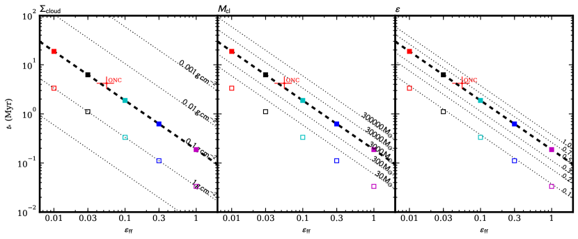
Figure 1: The star cluster formation timescale as a function of star formation efficiency per free-fall time ($\epsilon_{\rm ff}$) for the models presented in this work. In the first panel we show the dependence on different values of $\Sigma_{\rm cloud}$. As a reference, we mark $\Sigma_{\rm cloud}=0.1\,$g cm^-2 with a thick dashed line, and we show it in the second and third panels with its variation for different values of clump mass ($M_{\rm cl}$) and overall star formation efficiency ($\epsilon$), respectively. Square symbols show the models for which we performed simulations in this work with a color scheme used consistently for different values of $\epsilon_{\rm ff}$ in the following figures. The red point with errorbars shows the properties estimated for the ONC (Da Rio et al., 2014).

In Paper I we only simulated clusters in the “fast formation limit”, which means that star formation happened instantly and any residual gas also was expelled from the system instantly. In this paper, we now leave this approximation behind and acknowledge that stars are born gradually. Therefore natal gas is still present while stars are being formed. The presence of the gas, with a radial profile described by Eq. 1, is emulated by a time-dependent background potential, i.e.,

$$\Phi_{\rm gas}(r,t) = \left\{\begin{array}[]{lr}\dfrac{GM_{\rm cl}(t)}{(2-k_{\rho})R_{\rm cl}}\left[\left(\dfrac{r}{R_{\rm cl}}\right)^{2-k_{\rho}}-3+k_{\rho}\right]&,r\leq R_{\rm cl}\\ &\\ -\dfrac{GM_{\rm cl}(t)}{r}&,r>R_{\rm cl}\end{array}\right.,$$ (9)

where $G$ is the gravitational constant and $M_{\rm cl}(t)$ the time-dependent clump gas mass. Note that the radius of the clump is truncated at $R_{\rm cl}$ and therefore we do not include any effects of additional gas mass beyond this radius. Since the background gas is modeled with a smooth analytic potential, we also do not include effects such as dynamical friction caused by sub-structured gas acting on the stars.

In this paper we assume a constant star formation rate (SFR) defined using the initial parameters of the clump, i.e.,

$$\dot{M}_{*} = \frac{\epsilon_{\rm ff}M_{\rm cl,0}}{t_{\rm ff,0}}.$$ (10)

As stars are formed, some gas is assumed to be ejected from the system instantly according to a given local star formation efficiency, $\epsilon_{*}$, defined as the ratio between the stellar mass formed and the total mass required to form such a stellar mass. The fiducial value we adopt for $\epsilon_{*}$ is 0.5. This can be viewed as the star formation efficiency from an individual self-gravitating core, with the remainder of the core’s gas assumed to be ejected quickly from the clump by local feedback, expected to be dominated by protostellar outflows (see, e.g., Tanaka et al., 2017).

The time-evolution of the global gaseous mass of the clump is thus given by:

$$M_{\rm cl}(t) = \left\{\begin{array}[]{lr}M_{\rm cl,0}-\dfrac{\dot{M}_{*}}{\epsilon}t&,t\leq t_{*}\\ &\\ 0&,t>t_{*}\\ \end{array}\right.$$ (14)

where $t_{*}$ is the time at which gas is exhausted. Since we use a constant SFR and $\epsilon$, Equation 14 takes a linear form and the gas exhaustion time is simply $t_{*}=(\epsilon/\epsilon_{\rm ff})\times t_{\rm ff,0}$.

However, the value of $t_{\rm ff,0}$, defined as $\sqrt{3\pi/32\bar{\rho_{\rm 0}}}$, depends on $\Sigma_{\rm cloud}$ and $M_{\rm cl,0}$ since these values determine the size of the clump and therefore its mean density. Using the definition of $R_{\rm cl}$ (Eq. 2.1), the initial global free fall time reduces to:

$$t_{\rm ff,0} = 0.107\left(\frac{A}{k_{\rm p}\phi_{P,cl}\phi_{\bar{P}}}\right)^{3/8}\left(\frac{M_{\rm cl,0}}{3000\,{M_{\odot}}}\right)^{1/4}$$

$$\times\left(\frac{\Sigma_{\rm cloud}}{1\,{\rm g\,cm^{-2}}}\right)^{-3/4}\,{\rm Myr}$$

$$\rightarrow 0.069\left(\frac{M_{\rm cl,0}}{3000\,{M_{\odot}}}\right)^{1/4}\left(\frac{\Sigma_{\rm cloud}}{1\,{\rm g\,cm^{-2}}}\right)^{-3/4}\,{\rm Myr}.$$

Figure 1 shows the variation of $t_{*}$ given a different choice of initial parameters such as $\Sigma_{\rm cloud}$ (left) , $M_{\rm cl}$ (middle) and SFE (right) as a function of $\epsilon_{\rm ff}$ when keeping all other variables as constants. High $\Sigma_{\rm cloud}$ results in shorter free-fall times and therefore $t_{*}$ is smaller for the same $\epsilon_{\rm ff}$. We highlight the case $\Sigma_{\rm cloud}=0.1\rm\,g\,cm^{-2}$ (thick dashed line) and take it as reference line in the next two panels. The variation with the mass of the clump is less obvious: the size of the clump scales with mass as $R_{\rm cl}\propto M_{\rm cl}^{1/2}$ in order to keep the clump in equilibrium. The density of the clump scales linearly with the mass, this results in the relation $\bar{\rho}_{0}\propto M_{\rm cl}/R_{\rm cl}^{3}\propto M_{\rm cl}^{-1/2}$. And then $t_{\rm ff}\propto\bar{\rho_{0}}^{-1/2}\propto M_{\rm cl}^{1/4}$. The third panel shows the linear relation between $t_{*}$ and the SFE, which simply means that if the SFE is high, more mass will be converted into stars and therefore more time is needed to obtain the final stellar mass.

In the model presented here, one of the main assumptions in the star cluster formation scheme is that the SFR is constant with time, i.e., parameters such as $t_{\rm ff}$ and $\epsilon_{\rm ff}$ are defined based on the initial state of the clump. We note, however, that as stars are being born and the gas is being ejected/exhausted, the total (stars$+$gas) mass density decreases (eventually by a factor of two in the fiducial case) and so the free fall time becomes longer by a factor of $2^{1/2}$. Thus if the instantaneous value of $\epsilon_{\rm ff}$ were held fixed, i.e., a fixed fraction of gas converted into stars per local total free fall time, then the SFR would taper off towards zero (see, e.g. Parmentier & Pfalzner, 2013). However, given our desire to first explore simplest models, we will defer exploring such varying SFR cases until a future paper. We note also that observational values of $\epsilon_{\rm ff}$ (e.g., Da Rio et al., 2014) are based on time averaged SFRs.

2.2 Gradual formation of stars

In order to simulate the birth of stars in a cluster at different star formation rates, we have developed a modified version of the direct $N$-body code Nbody6++ (Aarseth, 2003; Wang et al., 2015). We introduced routines in order to add particles during run-time, including formation of primordial binaries. The introduction of stars is carried out as follows: (1) We create the final phase-space distribution of stars following the model described in Paper I. (2) The set of particles is unsorted creating the formation sequence. The used unsort method ensures that the global binary fraction is preserved at all times if no binaries are lost during the simulation. (3) We select an initial set of $N_{\rm i}=150$ particles from the list that are introduced in the simulation as usual, i.e., as the initial cluster, which is a small fraction of the eventual total. (4) For each particle in the subsequent list, the time needed for its formation is calculated as $t_{\rm*,i}=m_{\rm i}/{\rm SFR}$ and the cluster is evolved until $t+t_{*,\rm i}$ when the particle is born. This step is repeated until there is no more gas available. Binaries are always added together, and the time necessary for the formation of a binary is given by its total mass.

As in Paper I, stellar mass loss from stellar evolution is included in the simulations using the analytical models developed by Hurley et al. (2000, 2002) implemented in Nbody6++. We also include artificial velocity kicks from asymmetrical supernovae ejections. The magnitude of the velocity kicks follows a Maxwellian velocity distribution with $\sigma=265$ km/s based on proper motion observations of runaway pulsars (Hobbs et al., 2005) and the same velocity kick distribution is used for neutron stars and black-holes. With this high velocity kick distribution most black-holes and neutron stars are ejected from the system (Pavlík et al., 2018) and therefore dynamical effects caused by these objects are negligible.

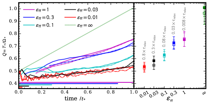
(a) Virial ratio

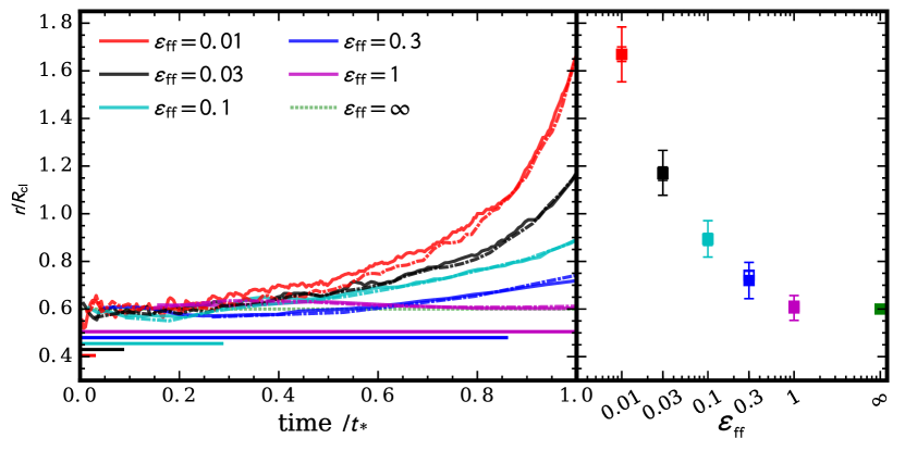
(b) Half mass radii

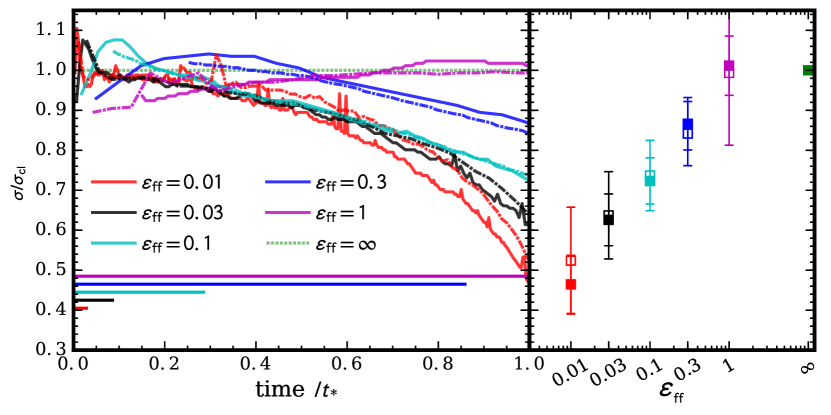
(c) Velocity dispersion

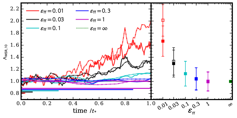
(d) Mass segregation parameter

Figure 2: Evolution of the virial ratio (a), half-mass radius (b), velocity dispersion (c) and mass segregation parameter based on ten most massive stars (d) during the formation of the star clusters for different values of $\epsilon_{\rm ff}$. Low-$\Sigma$ case is drawn with solid lines and High-$\Sigma$ with dot-dashed lines. The time is normalized by the duration of the star-forming stage, $t_{*}$. For reference, for each value of $\epsilon_{\rm ff}$, the length of a crossing time is drawn as an horizontal line in the bottom of the panel. In the $\epsilon_{\rm ff}=1$ case (magenta lines), $t_{*}\approx 0.4t_{\rm cross}$, so this line extends beyond the range shown in the panels. Each value at the end of the formation stage is shown in the right respective panels as a function of $\epsilon_{\rm ff}$. High and Low-$\Sigma$ cases are represented with open and filled squares respectively. Errorbars show the standard deviation of the mean values over the 20 realizations performed for each set. In panel (a), each point is labelled with the length of $t_{*}$ in terms of the relaxation time of the system using the final number of stars.

2.3 Overview of the Cluster Models

In this work, we make exactly the same assumptions for the stellar distribution of stars in space and in velocity structure as in Paper I. We assume stars are formed from the turbulent clump of gas, and therefore they follow the same global structure given by Equations 1 and 2. We test the parent clumps in two extreme scenarios with $\Sigma_{\rm cloud}=0.1$, and 1.0 g cm^-2 that we refer as high and low $\Sigma$ cases, respectively. In this paper we focus on the differences generated when varying the rate at which stars are formed as parametrized by $\epsilon_{\rm ff}$, for which the case of Paper I can be compared as $\epsilon_{\rm ff}\rightarrow\infty$. We focus on the fiducial set of simulations defined in Paper I (see Table 2), i.e., using a standard initial mass function (Kroupa, 2001) with a binary fraction $f_{\rm bin}$ with circular orbits. Binary properties are drawn from a log-normal period distribution with a mean of $P=293.3\,$yr and standard deviation of $\sigma_{\log P}=2.28$ (with $P$ in days) according to observations of Raghavan et al. (2010). The mass ratio distribution follows the form $dN/dq\propto q^{0.7}$ as observed in young star clusters (Reggiani & Meyer, 2011). We test values of $\epsilon_{\rm ff}=$ 0.01, 0.03, 0.1, 0.3, and 1, adopting $\epsilon_{\rm ff}=0.03$ as a fiducial value.

In this work, we deviate from the fiducial case only to see differences of two extremes: the binaries_100 case with 100% binaries and the segregated case where stars are radially sorted based on mass, which emulates an extreme case of mass segregation. However, these cases are only tested against the fiducial value of $\epsilon_{\rm ff}$.

A summary of the initial conditions is shown in Table 2, as well as the parameters chosen for the parent clumps in Table 1.

3 Results

3.1 Star cluster formation stage

The main difference between this and most previous $N$-body studies, is that we recreate the formation stage of star clusters by gradually adding stars during the simulation. Since the phase-space distribution of the stars follows the structure of the gas, this causes that star clusters are born with a dynamical structure that does not represent a stellar system in dynamical equilibrium. Even though the virial ratio of a system with SFE of 100% would be $Q=0.5$ (see Figure 1 of Paper I), the system is not in equilibrium since the velocity structure of the gas (a velocity dispersion that increases with the central distance) is the opposite of a dynamically stable stellar system (for which the velocity dispersion decreases with radius). Thus a longer formation timescale (i.e., lower $\epsilon_{\rm ff}$) can be crucial for the star cluster in order to rearrange internally before residual gas is dispersed, and therefore start its gas free evolution closer to equilibrium.

Figure 2a shows the evolution of $Q$, i.e., degree of gravitational boundedness, with time during the formation stage for the different values of $\epsilon_{\rm ff}$ adopted in this work. The time is normalized by $t_{*}$ (see Table 2), and for reference we also show the length of a crossing time for each value of $\epsilon_{\rm ff}$ in this normalization. Initially all systems start their evolution close to $Q=0.5$ since all the mass of the clump is present. As the cluster evolves, the stars that are present attempt to relax to equilibrium as more stars arrive with the relatively high velocity dispersion fixed from the initial conditions and the mass of the gas decreases. However, the initially small stellar cluster needs about one relaxation time ($t_{\rm relax}\sim 50\,t_{\rm cross}$ in the systems studied here) to reach equilibrium. The duration of star cluster formation in the fast regime, $\epsilon_{\rm ff}>0.1$, is comparable to the crossing time of the system. In this short time the star cluster is unable to reach equilibrium and the consequence is that it emerges from the gas with supervirial velocities. In contrast, in the slow regime $\epsilon_{\rm ff}\ll 0.1$, i.e., with slow star formation, the timescale is comparable to the relaxation time, and the stellar cluster has plenty of time to approach towards equilibrium. In this scenario, the formation of the star cluster is a race to reach equilibrium, and the path to equilibrium is truncated when the gas is gone and the cluster emerges from its natal clump with a global virial ratio given by this truncation (see right panels of Figure 2). Here the two extreme values of $Q$ that a cluster is able to reach at the end of its formation are $Q\simeq 0.5$ when $t_{*}\gtrsim t_{\rm relax}$ and $Q\simeq 0.75$ when $t_{*}$ is relatively short, with a limit of $Q\simeq 1$ in the instantaneous formation case of Paper I.

Figure 2b shows that the rearrangement of the stars into a relaxed configuration implies that the cluster expands even before all gas is exhausted. While the star-forming region, i.e., the clump of gas, is forced to remain with the same size, a considerably amount of stars start orbiting the system outside the clump. Long orbits also means low velocities and the overall velocity dispersion of the cluster decreases, as shown in Figure 2c. As shown in these panels b and c, how much the cluster expands and the velocity dispersion decreases is highly dependent on the assumed $\epsilon_{\rm ff}$. In the slowest formation scheme tested here, $\epsilon_{\rm ff}=0.01$, the half mass radius of the cluster expands a factor of 2.6 and the velocity dispersion decreases by a factor 2 compared to the initial values. However in the fastest cases $\epsilon_{\rm ff}=1$ and $\infty$, the initial values are not modified at all. This result is independent of $\Sigma_{\rm cloud}$.

We have also followed the evolution of mass segregation during the formation stage. We quantified mass segregation using the mass segregation ratio $\Lambda_{\rm MSR}$ introduced by Allison et al. (2009a). $\Lambda_{\rm MSR}$ is defined as the ratio between the length of the minimum spanning tree (MST) connecting the $N_{\rm MST}$ most massive stars in the cluster ($l_{\rm massive})$, which is unique) and the MST connecting $N_{\rm MST}$ randomly selected stars ($l_{\rm normal}$). The latter is done 500 times in order to have good estimations of the dispersion in $l_{\rm normal}$, $\sigma_{\rm norm}$, then:

$$\Lambda_{\rm MSR}\equiv\frac{\langle l_{\rm normal}\rangle}{l_{\rm massive}}\pm\frac{\sigma_{\rm normal}}{l_{\rm massive}}$$ (16)

where $\Lambda_{\rm MSR}\sim 1$ means no mass segregation and $\Lambda_{\rm MSR}>1$ indicates a mass segregated star cluster, i.e., massive stars are more closely distributed than other stars. For our numerical evaluations of $\Lambda_{\rm MSR}$ we adopt $N_{\rm MST}=10$.

In our fiducial models with different values of $\epsilon_{\rm ff}$, the star clusters are created without primordial mass segregation. Figure 2d shows how in all cases $\Lambda_{\rm MSR}=1$ at $t=0$ and mass segregation gradually develops as time progresses. The level of mass segregation that star clusters are able to reach at the end of star formation thus depends on $\epsilon_{\rm ff}$. Mass segregation is developed dynamically as massive stars sink to the center and kick out lower mass stars. Numerical studies have shown that star clusters can develop significant mass segregation on timescales $<1$ Myr with (Domínguez et al., 2017) and without background gas (Allison et al., 2009b). In these studies, fast segregation is normally explained by the means of high levels of primordial substructure and sub-virial velocities involving the merging of subclumps of stars. Figure 2d shows that longer formation timescales develop high levels of mass segregation, and this result is independent of the initial density. The only exception appears in the case of $\epsilon_{\rm ff}=0.01$ (red lines) where in the low $\Sigma$ case stellar evolution affects the result as massive stars die truncating the growth of segregation. However, in all other cases the result is the same, low values of $\epsilon_{\rm ff}$ implies more crossing times in a dense state and more time for developing mass segregation.

In agreement with previous studies, with our spherically symmetric models that have minimal substructure, we are not able to develop very high levels of mass segregation in $<1$ Myr, even in the high density cases. The case where mass segregation developed most was in the high-$\Sigma$ case with $\epsilon_{\rm ff}=0.01$. Here star clusters reached $\Lambda_{\rm MSR}=2$ but it takes $t_{*}\approx 3$ Myr to develop it. Future improvements of our modeling will include the addition of primordial substructure and we will be able to study how fast mass segregation can be developed in different density environments and formation timescales.

3.2 Emergence from the gas

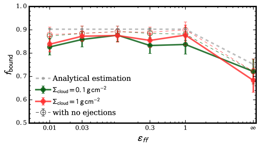
Figure 3: Bound mass fraction measured at the time at which the gas is exhausted ($t_{*}$), for simulations in the fiducial set in the high (red) and low (green) $\Sigma$ cases. Gray dashed line shows a semi-analytical estimation (see §A). Each point with errorbars represents the mean and standard deviation for 20 simulations. Thin lines with open symbols show the resulting bound fractions, if dynamical ejections are counted as bound, for comparison with the analytic model.

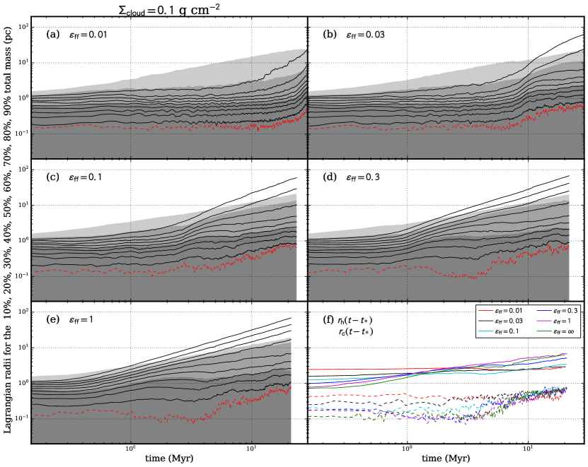
Figure 4: Time evolution of average Lagrangian radii for star clusters born from a parent clump with $\Sigma_{\rm cloud}=0.1\>{\rm g\>cm^{-2}}$ and for various values of $\epsilon_{\rm ff}$, as labelled in panels (a) to (e). We show the Lagrangian radii for the 10%, 20%, 30%, 40%, 50%, 60%, 70%, 80% and 90% masses (black solid lines). Red dashed lines are the core radii defined in Aarseth (2003). Gray shaded areas represent the regions below the 50%, 95% and 100% mass radius of the bound cluster. Panel (f) shows the half-mass and core radii of all the clusters together, including the $\epsilon_{\rm ff}=\infty$ case.

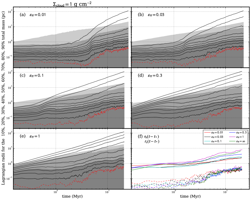
Figure 5: Same as Figure 4 for star clusters born from a clump with $\Sigma_{\rm cloud}=1\>{\rm g\>cm^{-2}}$.

Figure 3 shows the different values of bound fraction ($f_{\rm bound}$) at $t=t_{*}$. While there are some differences between the models, that we discuss below, in general there is only modest variation of $f_{\rm bound}$ for different values of $\epsilon_{\rm ff}$. The different values of $Q$ obtained at the end of the formation stage, between $0.5<Q<0.8$, would suggest different bound fractions (see e.g. Farias et al., 2018; Lee & Goodwin, 2016), however the differences in this narrow range are quite small. Second order differences are a combination of dynamical effects such as early dynamical ejections and the assumptions of the formation process, e.g., the different rates of decrease of the gas mass.

Let us first ignore early dynamical effects such as virialization and the rearrangement of the stellar masses. In this regime, the sequential formation of stars does not affect the final bound fraction. As each star is formed the escape velocity decreases in the same amount instantly. Therefore, how fast or slow stars are created becomes irrelevant because of the instant residual gas loss assumed in this work. Gray dashed lines on Figure 3 show an analytical estimation considering the radial and time dependent escape velocity and clump velocity distribution based on the cloud model described in §2.1 (see Appendix A for details). Thin lines with open symbols in Figure 3 show the resulting bound fractions when only removing stars that are born unbound, i.e., ignoring dynamical ejections, and we can see that the analytic estimations and numerical experiments agree well.

Then, the actual bound fraction is shown by the solid lines with solid circles in Figure 3. Values of $\epsilon_{\rm ff}=0.1$ and 0.3 (low $\Sigma$) show slightly lower bound fractions, probably due to the combination of the higher virial ratios and dynamical ejections that happen during formation. Then, at low values of $\epsilon_{\rm ff}<0.1$ there are also slightly smaller bound fractions: in this case, dynamical ejections play an important role during formation, since it happens on several ($\gtrsim 10$) crossing times. It is at $\epsilon_{\rm ff}=0.1$ where both effects appear to be minimized.

3.3 Global evolution

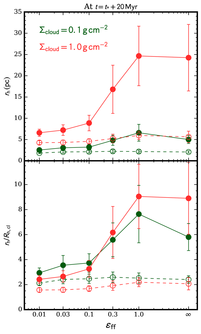
Figure 6: Size of star clusters at 20 Myr after star formation stops. The top panel shows the half-mass radius in parsecs. The bottom panel shows the half-mass radius relative to the initial clump size ($R_{\rm cl}$). Filled circles are the values measured with all stars in the clusters, while open circles are values measured only with the bound stars. The low (green) and high (red) $\Sigma_{\rm cl}$ cases are indicated (see legend).

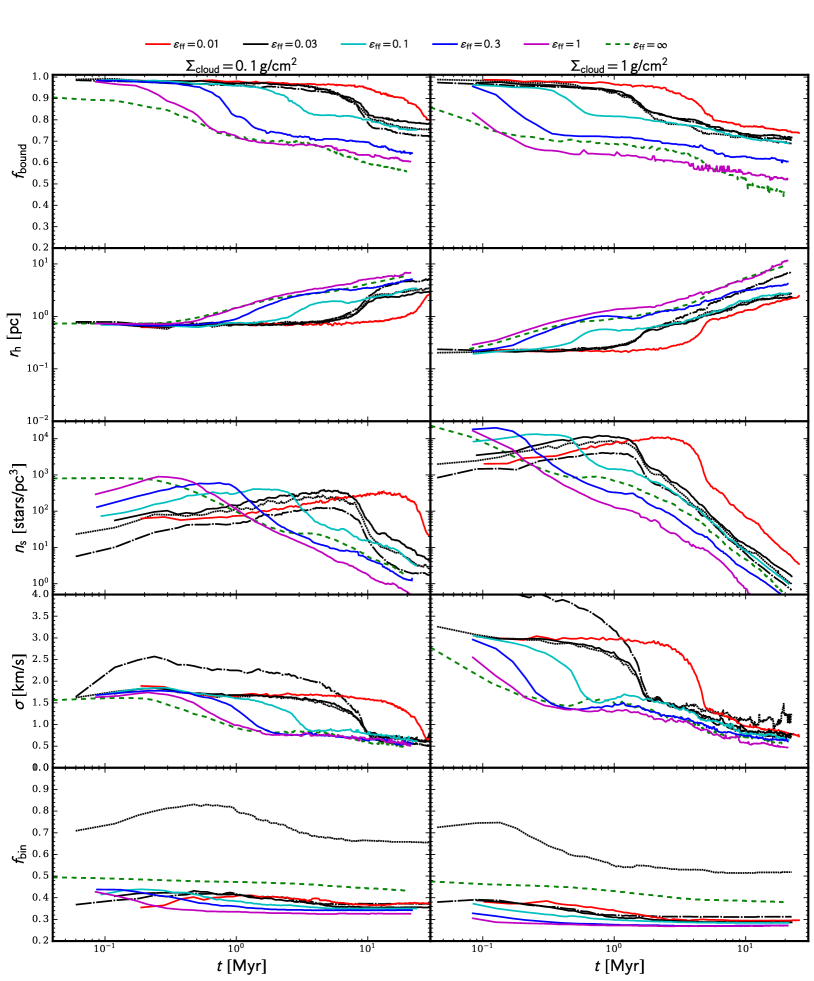
Figure 7: Time evolution of properties for our fiducial clusters formed with SFE=50% and a range of $\epsilon_{\rm ff}$ values in different colors (see legend). Solid lines show results for the fiducial set, dotted lines for the set binaries_100, dot-dashed lines for segregated and dashed lines the results of the fast formation limit described in Paper I. Left column shows clusters forming from a $\Sigma_{\rm cloud}=0.1$ g cm^-2 environment; right column from a $\Sigma_{\rm cloud}=1$ g cm^-2 environment. The lines in each panel show median values calculated from the 20 simulations performed for each set. Top row shows the fraction of bound mass in the cluster relative to the instantaneous stellar mass, where in this figure unbound stars inside the 95% mass radius of the bound cluster are kept to show the timescale of their escape. Second row shows the evolution of the half mass radius $r_{\rm h}$ for all the stars in the simulation. Third row shows the average number density of systems ($n_{s}$), where by systems we refer to singles and binaries, measured inside the volume defined by $r_{\rm h}$. Fourth row show the evolution of the velocity dispersion measured inside $r_{\rm h}$, and bottom row shows the evolution of the global binary fraction.

We have seen that one of the key effects of varying $\epsilon_{\rm ff}$ is the ability of the star cluster to reach equilibrium before gas is exhausted/ejected. While the difference in their ability to survive gas expulsion is not raised considerably, the condition on which they face their early gas-free evolution is very different. We have evolved every model for 20 Myr after all stars are formed. The global evolution under each model’s parameters can be appreciated through the Lagrangian radii shown in Figure 4 for the low $\Sigma$ case and in Figure 5 for the high $\Sigma$ case. Comparing between these mass surface densities, the differences are similar as found in Paper I: star clusters born with high density expand at a faster rate than star clusters born in a less dense state. However, the expansion is also regulated by the star formation rate.

Panel (f) of Figures 4 and 5 shows the half mass and core radii for all the values of $\epsilon_{\rm ff}$ with a time offset so that the starting point is the moment when they start their gas free phase, i.e., $t-t_{*}$. High values of $\epsilon_{\rm ff}$ result in star clusters that expand much faster than the ones born with low $\epsilon_{\rm ff}$. As we can extract from Figure 6, where we compare the half mass radii at 20 Myr after formation, the extreme cases are when star clusters are born with low density and low $\epsilon_{\rm ff}$ and do not expand at all following the expulsion of gas (they only expand initially a factor 2 during the formation stage, see Figure 2). On the other hand, a star clusters born in one free fall time ($\epsilon_{\rm ff}=1$) expands by a factor 9 during the first 20 Myr.

A summary of the evolution of different parameters is shown in Figure 7. Including the evolution of the extremely mass segregated case (segregated set, in dot dashed lines), and the set with 100% binaries (binaries_100, shown in dotted lines), withe the low $\Sigma$ case in the left panels and high-$\Sigma$ case in the right.

Top panels show the evolution of the bound fraction. As discussed in §3.2, at $t_{*}$ the fraction of bound stars is similar at all $\epsilon_{\rm ff}$. However, $t_{*}$ is different for each set and since $f_{\rm bound}$ evolves due to dynamical ejections, at a fixed time, e.g., $t_{\rm m}=10$ Myr, the bound stellar fraction is very different in each case. If we take a fixed physical time as a reference, then we can say that star clusters born slowly better survive gas exhaustion than star clusters that form fast. However, this is because the formation time ($t_{\rm*}$) is different for each set and a fixed physical time does not represent the star clusters in the same state. Most of the stellar mass loss is during the star formation phase due to dynamical ejections in a high density state and stars being born unbound from the cluster (see Section 3.7), but after the gas is gone, dynamical ejections are still happening, and therefore, if we compare at a fixed physical time ($t_{\rm m}$), we will count the mass loss during the formation plus the mass loss during the time $t_{\rm m}-t_{*}$. If we compare the bound fraction at the end of star formation in each case as shown in Figure 3, we see that the difference between the models is not significant. Extreme cases such as segregated and binaries_100 do not show significant deviations.

Second row panels show the evolution of stellar half mass radius in physical time. We showed in §3.1, slow-forming star clusters expand more during formation but after gas is gone they are more stable against further expansion. However, since their formation stage takes longer, slow-forming clusters are more compact at any time in their evolution when comparing to star clusters formed fast at the same time. While the binaries_100 set expands at the same rate as the fiducial set, the segregated set expands faster since the velocity dispersions remain high due to the large amounts of close massive stars. A direct consequence of the evolution of $r_{\rm h}$ is the evolution of the system number densities ($n_{\rm s}$) within $r_{\rm h}$, shown in the third row. By system we refer to single and binary stars, therefore the binaries_100 set have slightly smaller number densities than the fiducial set. Also, since in the set segregated more massive stars are in the center, then there are fewer stars born in the center in order to follow the density profile of the parent clump. The difference in $n_{\rm h}$ due to these effects remains during the whole evolution of the cluster. Overall, $n_{\rm h}$ is high during the formation of stars and increases as new stars are born, then when the gas is gone and star clusters start to expands $n_{\rm h}$ fall several orders of magnitude in all sets.

The fourth row of panels shows the evolution of the velocity dispersion within $r_{\rm h}$, $\sigma_{\rm h}$. Velocity dispersions are high during the formation of stars, since the background gas is present, and after gas is gone it falls until an equilibrium value is established that is similar for all the models. Later decrease of $\sigma_{\rm h}$ is relatively small and would be very difficult to distinguish between the models. Note, $\sigma_{\rm h}$ depends on the total density of the cluster, but its variation is small when the initial mass of the system, $M_{\rm cl}$ falls by a factor of 0.5, i.e., $\epsilon$. In the set segregated, $\sigma_{\rm cl}$ rises rapidly as all massive stars are close to each others, however, after the rearrangement of the stellar distribution, the final value of $\sigma_{\rm cl}$ is the same as the other models.

The last row of panels shows the evolution of the binary fraction. Within the models, the evolution of the binary fraction is similar, however in all cases studied here, there is more disruption of binaries than in the case studied in Paper I. This is because in the cases here, the number densities stay higher for longer, and most binaries have a reasonable chance to interact with the other stars. However in the fast formation limit, the cluster starts its life in expansion, not allowing much interaction between them and the rest of stars. Binary stars are introduced uniformly over time, however, binary stars are disrupted very early and the binary fraction evolves to a smaller number than that given by the initial conditions. We discuss the binary population in the next section.

3.4 Binary population

$\begin{array}[]{rl}\includegraphics[width=216.81pt]{ebinhist.pdf}&\includegraphics[width=216.81pt]{ebinhistss1.pdf}\end{array}$

Figure 8: The probability distribution functions (PDF) of binary binding energies. Top panels shows the PDFs measured at 20 Myr with the shaded area representing the distribution of the initial conditions given to binaries when they form. Bottom panels show the differences in the PDFs in comparison with the initial population. The left column shows the result for clusters in the low mass surface density environment ($\Sigma_{\rm cl}=0.1\>{\rm g\>cm^{-2}}$); the right column shows the high mass surface density environment ($\Sigma_{\rm cl}=1\>{\rm g\>cm^{-2}}$).

$\begin{array}[]{rl}\includegraphics[width=216.81pt]{ecchist.pdf}&\includegraphics[width=216.81pt]{ecchistss1.pdf}\end{array}$

Figure 9: Fraction of binaries in each $\Gamma_{\rm b,eff}$ bin that were disrupted (lines with errorbars) and for which the initial eccentricity changed by $\Delta e>0.1$ (hatched histograms). The grey filled histogram shows the actual fraction of binaries in each bin. Most binaries with high $\Gamma_{\rm b,eff}$ are disrupted, however note that there are only a small fraction of binaries in this regime. Thus, overall the changes in the binary populations are relatively modest, but at high $\Gamma_{\rm b,eff}$ the evolution is significant, including some dependence on $\epsilon_{\rm ff}$.

In the models presented here we have included a relatively high (50%) percentage of primordial binaries (though note this value is compatible with observational estimates). Binary population parameters in this work are the same as in Paper I. In Paper I we did not find that there was significant dynamical processing of primordial binaries. Now in the models with gradual star formation, as star cluster formation last longer, the chance that a binary system has to interact with others increases since number densities stay higher for longer. Therefore we would expect that the degree of dynamical processing increases with lower values of $\epsilon_{\rm ff}$. Indeed, this is what we see from Figure 8, where we compare the initial distribution of binding energies (shown by grey filled histograms) with the same distribution measured at 20 Myr for the different values of $\epsilon_{\rm ff}$. The differences between initial and evolved distributions are shown in the bottom panels. In general the Heggie-Hut rule is followed as hard binaries become harder and soft binaries become softer with time, causing the peak of the PDF to move to the left. In the high $\Sigma_{\rm cl}$ case (right panels) the differences between models is greater, where low $\epsilon_{\rm ff}$ values results in larger modifications of the initial PDF. In the low $\Sigma_{\rm cl}$ cases the differences are less prominent, even though the same trend is still present.

However, the above results will depend on the adopted initial binary population. In Paper I, we calculated the interaction rates of interactions with cross sections on the order of the separation of the binary stars as:

$$\Gamma_{\rm b,eff} = \Gamma_{\rm b}\cal{F}$$ (17)

where $\Gamma_{\rm b}$ is the interaction rate factor given by:

$$\Gamma_{\rm b}(a,\mu) \lesssim 9.67\times 10^{-3}\left(\frac{n_{s}}{10^{4}\>{\rm pc}^{-3}}\right)\left(\frac{\sigma}{2~{}{\rm km\,s^{-1}}}\right)$$

$$\times \left(\frac{a}{40~{}{\rm AU}}\right)^{2}\frac{\langle m_{s}\rangle^{2}}{\mu^{2}}\>{\rm Myr}^{-1}\quad,$$ (18)

where $a$ is the binary semi-major axis, $\mu=m_{1}m_{2}/(m_{1}+m_{2})$ is the reduced mass of the binary with components of masses $m_{1}$ and $m_{2}$. And $\langle m_{\rm s}\rangle$ is the average system mass, which in a system with a binary fraction $f_{\rm bin}$ and average mass $\langle m_{i}\rangle$ this is $\langle m_{\rm s}\rangle\approx(1+f_{\rm bin})\langle m_{i}\rangle$, ignoring the presence of higher order multiple systems. The inequality comes from the fact that the derivation of $\Gamma_{\rm b}$ assumes that if the perturber is a binary, then its semimajor axis is smaller or similar to the binary in question, which normally holds for soft binaries but not usually for the hard ones. Gravitational focusing effects are accounted by the factor $\cal{F}$ in Eq. 17 given by:

$$\cal{F} \approx 1+\left[5.55\left(\frac{\mu}{{M_{\odot}}}\right)\left(\frac{a}{40\>{\rm AU}}\right)^{-1}\left(\frac{\sigma}{2\>{\rm km/s}}\right)^{-2}\right.$$ (19)

$$\times\left.\left(\frac{m_{1}+m_{2}}{m_{s}}+1\right)^{\vphantom{1}}\right].$$

While these interaction rates change as the cluster evolves and the internal properties of the binary systems change with each interaction, it serves as a good estimator of which stars are most likely to be perturbed during the simulations. The grey histograms of Figure 9 show the fraction of binary stars in each logarithmic $\Gamma_{\rm b,eff}$ bin, given the chosen primordial binary population properties. In Paper I we explored how initial eccentricities changed as a function of $\Gamma_{\rm b,ff}$. First we considered the fraction of binaries that have their eccentricities modified by a 1% change or greater. This fraction increases with $\Gamma_{\rm b,eff}$ until reaching a level of about 20% by $\Gamma_{\rm b,eff}=1\,{\rm Myr}^{-1}$, after which it remains flat.

Now in the models of gradual cluster formation, with longer formation timescales we expect a larger fraction of modified eccentricities for $\Gamma_{\rm b,eff}>1$ Myr^-1. However, as we can see from the hatched histograms of Figure 9 this does not happen, instead the fraction of modified eccentricities decreases with larger $\Gamma_{\rm b,eff}$. The explanation is that so far we did this analysis considering only binary stars that remained bound after 20 Myr. However, if we analyse the fraction of binaries that were disrupted in each $\Gamma_{\rm b,eff}$ bin (see solid lines with Poisson errorbars in Figure 9) we can see that this increases very strongly with $\Gamma_{\rm b,eff}$. In fact, at the highest values of $\Gamma_{\rm b,eff}$, i.e., $\gtrsim 4\>{\rm Myr}^{-1}$, the majority of binaries are disrupted and those that are not almost all have had their eccentricities modified by at least 1%.

However, even though the fraction of perturbed binaries is high at large values of $\Gamma_{\rm b,eff}$, only a small fraction of binary systems reach these high interaction rates. It remains to be explored to which extent the binary population can be dynamically processed in these models, if we choose different primordial binary populations with different formation timescales.

3.5 Radial structure

$\begin{array}[]{c}\includegraphics[width=433.62pt]{diff_density.pdf}\\ \includegraphics[width=433.62pt]{diff_densityss1.pdf}\end{array}$

Figure 10: Evolution of the average radial stellar density profile of the clusters forming in the low (top panels) and high (bottom panels) $\Sigma_{\rm cl}$ environments, with the different values of $\epsilon_{\rm ff}$ indicated in the legends. Evolution is given after the star formation ends, i.e., setting $t_{*}$ as the starting point. Step functions show the measured profiles while the solid black line shows a fitting function to the fiducial $\epsilon_{\rm ff}=0.03$ case that we use for comparisons. The fitting function is a two part function (see text) and we show the continuation of the first part with a black dashed line. Auxiliary bottom panels shows the residuals of every model with respect to the $\epsilon_{\rm ff}=0.03$ fitting function in order to better see the differences between the models. Best fitting parameters are shown in each panel.

$\begin{array}[]{c}\includegraphics[width=433.62pt]{diff_surface_density.pdf}\\ \includegraphics[width=433.62pt]{diff_surface_densityss1.pdf}\end{array}$

Figure 11: Same as Figure 10 but for the surface density profile.

$\begin{array}[]{c}\includegraphics[width=433.62pt]{diff_dispersion.pdf}\\ \includegraphics[width=433.62pt]{diff_dispersionss1.pdf}\end{array}$

Figure 12: Evolution of the one dimensional velocity dispersion profile after star formation has ended for star clusters forming in the low (top panels) and high (bottom panels) $\Sigma_{\rm cl}$ cases. The values of the corresponding $\epsilon_{\rm ff}$ are shown in the legends. Velocity dispersions are measured treating stellar binaries as unresolved systems, in order to avoid contamination from the high velocities coming from their binary orbits.

The radial structure of star clusters, in their projected forms, are one of the most direct observables of real star clusters. We have first measured the average radial profiles for the 3D stellar mass density (Figure 10) and then its 2D projection, i.e., the stellar mass surface density profile (Figure 11), for both high and low-$\Sigma_{\rm cl}$ cases and at different times after star formation ended, i.e., at $t-t_{\rm*}=$ 0, 3, 10 and 20 Myr.

In order to better see the differences in the density profiles when varying $\epsilon_{\rm ff}$ we compare the models using $\epsilon_{\rm ff}=0.03$ as a baseline case using a fitting function to describe it. Density profiles obtained here show a different behaviour in the inner zones, dominated by the bound cluster, than in the outskirts, dominated by the unbound population. Then, the obtained profiles can be well described by a two part function of the form:

$$f(r) \propto \left\{\begin{array}[]{lr}r^{\alpha_{1}}\exp(\alpha_{2}r)&,r\leq r_{\rm crit}\\ &\\ r^{\alpha_{3}}&,r>r_{\rm crit}\\ \end{array}\right.$$ (23)

with $\alpha_{1}$, $\alpha_{2}$ and $\alpha_{3}$ fitting constants, $r$ in units of parsecs and $r_{\rm crit}$ the critical radius at which the $\alpha_{3}$ power law becomes a better description. Bottom auxiliary panels of Figures 10 and 11 show the residuals with respect to Eq. 23 fitted to the $\epsilon_{\rm ff}=0.03$ profiles.

One of the most obvious effects shown in these profiles is that just after star formation has finished the clusters that took the longest to form, i.e., low values of $\epsilon_{\rm ff}$ have more extended radial distributions. Note these include stars that were born unbound from the clump and those that become dynamically ejected.

We showed in Paper I that star clusters that form instantaneously exhibit a density excess in a surrounding “halo”, which is caused by a significant fraction of stars that were born unbound because of the initial high turbulent velocities. Since all of these stars were lost at the same time, this excess is quite prominent since they are at similar distances from the center. We can see in Figures 10 and 11 that as star cluster formation lasts longer, this excess becomes less prominent. In all simulations presented here there are stars that are born unbound from their natal regions, however, as they are born gradually they also leave the system gradually being more spread out in radial distance. They can also become mixed with stars that were dynamically ejected in the way. Therefore, one consequence of the models presented here is that star clusters forming slowly, should not have “bumps” in their density profiles.

We also have measured the evolution of the 1D velocity dispersion $\sigma_{\rm 1D}$ after star formation ended (see Figure 12). The first panel ($t=t_{*}$) clearly shows the consequence of a longer star formation timescale (low $\epsilon_{\rm ff}$) on the dynamical stability of the newly formed star cluster. At the end of the formation time, star cluster that formed quickly have a velocity profile of the parent cloud, i.e., increasing with radius (see green lines on Figure 12), while star clusters forming more slowly have a velocity dispersion profile that decreases with radius (see red lines). This is valid only for the bound part of the cluster and here any initial signature of the velocity dispersion profile is quickly erased after gas is expelled and the differences become very small. At large radii, where there are unbound stars, the velocity dispersion rises again because faster stars are farther from the cluster. Thus the velocity dispersion profile clearly shows the boundary where the bound cluster ends and the unbound population starts, i.e., where $\sigma$ has a minimum.

3.6 Age gradients

$\begin{array}[]{c}\includegraphics[width=433.62pt]{diff_age.pdf}\\ \includegraphics[width=433.62pt]{diff_agess1.pdf}\\ \begin{array}[]{rl}\includegraphics[width=173.44534pt]{fitages.pdf}&\includegraphics[width=173.44534pt]{fitagesss1.pdf}\end{array}\\ \end{array}$

Figure 13: Evolution of the average age radial gradients for the low (top panels) and high (middle panels) $\Sigma_{\rm cl}$ cases. Ages and radial distances are standarized, i.e., the mean value is subtracted and the result is divided by the standard deviation. Only stars within $3r_{\rm h}$ are considered in the analysis. A linear fit has been performed in the ranges $-1<r_{\rm std}<1$ and the resulting gradients are shown below each curve. Bottom panels show the evolution of these gradients in physical units.

One important feature of this work is that stars are born gradually during the simulations. This means that stars have different ages with an age spread equal to $t_{*}$. Stars are born uniformly in time and also in space but following the power law density profile of the initial clump gas. Therefore, in this work, we are able to look for radial age gradients that may form dynamically. In order to be able to compare with recent works on this matter, we have adopted the method used by Getman et al. (2018) who measured and compared age gradients in several young star clusters using standarized values for age and distance to the center. A given value, e.g., of age ($\tau$), is “standarized” by subtracting the mean of the sample and dividing the result by the standard deviation, i.e., for the $i$-th star:

$$\tau_{i,\rm std} = \frac{\tau_{i}-\langle\tau\rangle}{\sigma_{\tau}}$$ (24)

$$r_{i,\rm std} = \frac{r_{i}-\langle r\rangle}{\sigma_{r}}.$$ (25)

In order to avoid biasing results by stars that are very far from the cluster, e.g., because of dynamical ejections, that would increase the mean value of distance and standard deviation, we only consider stars within $3r_{\rm h}$ of the center of each cluster. This is also motivated by the fact that such stars are very difficult to associate observationally with a given cluster and would be normally not included in such studies.

The resulting radial profiles of average age are shown in Figure 13. In order to show the different gradients we perform linear fits in the standarized distances between -1 and 1. The resulting gradients are shown below the curves for clarity. At the end of star formation (left panels) there is a clear trend in which slower forming clusters show a steeper radial gradient of mean age, i.e., with younger stars in the center and older stars in the outskirts. For faster forming clusters (in fewer dynamical times) the gradient becomes flatter and even turns around for the case of $\epsilon_{\rm ff}=1$. The reason for these gradients is the expansion of the cluster during the formation stage. While the star-forming region is constrained to be within $R_{\rm cl}$ by the model assumptions, slow forming clusters expand during the formation phase as they move towards equilibrium, so older stars tend to be found in the outer regions. Such effects will generally occur in real systems if the star-forming region can be described as a localized dense gas clump.

As the cluster evolves without gas, this signature starts to decrease as stars (in the bound cluster) are mixed again and the gradient disappears. However, the gradients can remain strong for a considerable period of time. In the low $\Sigma_{\rm cl}$ case it is possible to still see the effects at 10 Myr, though for the high $\Sigma_{\rm cl}$ case, the signature disappear sooner because of the faster dynamical evolution implied by the high density.

The recent work of Getman et al. (2018) has concluded that age gradients are generally present in young star clusters and the majority ($\sim 80\%$) of these gradients are positive, i.e., younger stars in the core compared to the outskirts (see also Getman et al., 2014). In Figure 13 we show that slow forming star clusters tend to form more positive and steeper age gradients relative to fast forming clusters. In terms of physical units, (Getman et al., 2018) obtained gradients between 0.75-1.5 Myr pc^-1 depending on the model used to estimate stellar ages. In this work, we have been able to reach such values only with slow forming star clusters ($\epsilon_{\rm ff}<0.03$, as can be seen in the bottom panels of Figure 13. When transforming to physical units the difference between the models are amplified, given that slow forming clusters have larger age spreads by construction, and therefore can naturally form greater gradients. However, we note that the fundamental difference also appears in standarized units and use of physical units only amplifies the differences. Then, high $\Sigma_{\rm cloud}$ cases show smaller initial age gradients because $t_{*}$ is smaller. However, the rapid dynamical evolution of these systems also remove the gradients more quickly.

3.7 Ejected stars and kinematic structure

$\begin{array}[]{c}\includegraphics[width=433.62pt]{{fiducialSS_0.1sfe_ff003-scatter}.pdf}\\ \includegraphics[width=433.62pt]{{fiducialSS_1.0sfe_ff003-scatter}.pdf}\end{array}$

Figure 14: Normalized velocity versus stellar mass (left panels) and versus distance from cluster center (right panels) for all stars in the fiducial case with $\epsilon_{\rm ff}=0.03$ for simulations with $\Sigma_{\rm cloud}=0.1\>{\rm g\>cm}^{-2}$ (top) and $\Sigma_{\rm cloud}=1\>{\rm g\>cm}^{-2}$ (bottom), measured at 20 Myr. Stars are separated in three groups: bound stars (black); stars born unbound (green); and ejected stars (red). Velocity values are normalized by the mass-averaged velocity dispersion of the parent clump (see 2). Small top and side panels show the PDFs considering all stars in the set (gray shaded area), and the fraction of the PDFs that correspond to each group of stars (lines). An example velocity threshold of 20 km/s is shown by a green line.

Following our analysis of Paper I, we identify bound members in the simulations snapshot by snapshot, classifying stars in three groups: (1) bound stars, which are the ones that remain bound until the end of the simulation; (2) unbound stars, which were unbound from the first snapshot that they appear, i.e., they are born unbound; (3) Ejected stars, which are stars that appear bound in one snapshot but later they do not. With the ejected stars, we also subdivide them in: (A) Strong dynamical ejections, i.e., stars that show $\Delta T_{i}\geq 2\Delta\Omega_{i}$, when ejected; (B) Supernovae ejections, including stars receiving velocity kicks during their supernovae phase, and stars ejected because they were binary companions of a star that exploded as supernovae; and (C) gentle ejections, stars that become unbound because of the evolving potential of the cluster, which we distinguish by $\Delta T_{i}<2\Delta\Omega_{i}$. In this work, we refer to runaway stars, as dynamically ejected stars with velocities above 20 km/s, but note that this is an arbitrary threshold for such a definition.

Following the format of Paper I, we show the structure formed by these three groups of stars in the velocity-mass and velocity-distance diagrams in Figure 14, all measured at 20 Myr. Velocities are normalized by $\sigma_{\rm cl}$ of the parent clump (see 1 and the 20 km/s threshold is marked as a green horizontal line for reference. The corresponding PDFs are shown in the respective side panels. The structures formed in the velocity-distance diagrams are similar to those in Paper I, however the number of stars that born unbound (green) has decreased considerably and these are a smaller fraction of the corresponding final PDFs. The population of ejected stars (red) is stronger in these models, however they are now spread over a wider range of distances and velocities. This is a consequence of the large and slow decrease on the escape velocity of the system and the spread in the formation times of the stars.

$\begin{array}[]{rl}\includegraphics[width=216.81pt]{ejectionssigma0p1.pdf}&\includegraphics[width=216.81pt]{ejectionssigma1.pdf}\end{array}$

Figure 15: Average dynamical ejection rates for star clusters in the fiducial set with different values of $\epsilon_{\rm ff}$. As a reference of the cluster structure, bottom panels show the time evolution of the number density inside the half mass radius of the cluster.

We also recorded the time when strong ejections happen and we measured the dynamical ejection rate, shown in Figure 15 for the low (left) and high (right) $\Sigma_{\rm cloud}$ cases. During the formation of the clusters, the ejection rate remains higher and is closely correlated to the number densities (shown in the bottom panels). As stars are formed, the central number densities grow, along with the ejection rates. The peak density in the different models, which is reached at the end of the formation stage, is smaller at low $\epsilon_{\rm ff}$. As we saw in §3.3, star clusters expand more during formation when $\epsilon_{\rm ff}$ is small, and therefore the peak number density is also smaller than in the high $\epsilon_{\rm ff}$ regime. This difference causes the peak in ejection rate to be smaller at low $\epsilon_{\rm ff}$, but significantly broader. After gas is gone and the cluster expands, ejection rates fall at a similar rate in all models.

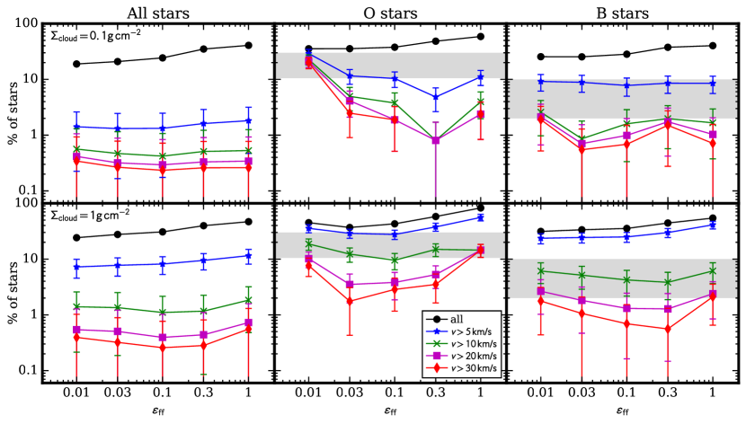
Figure 16: Percentage of ejected stars relative to all stars in each mass range for results for the low (top panels) and high (bottom panels) $\Sigma_{\rm cloud}$ cases. The first column shows the results when using all stars in the set, center panels when considering only O stars and left panels for B stars. Different colors shows different velocity thresholds to define “ejected” and gray shaded areas the range of values found in the literature for runaway stars under various definitions (see text).

Figure 17: Velocity (top panels) and kinetic energy (bottom panels) distributions of ejected stars, shown as the probability of finding an ejected star with velocity or energy above a given value.

Figure 16 (left column) shows the collected percentage of ejected stars in each simulation set, including for various threshold velocities that can be used to define “runaways”. Then the middle and right columns show the same results, but for O and B stars, respectively. Note, these are only dynamically ejected stars via $3+$-body interactions and not those ejected due to binary supernova explosions. Filled black circles show the total percentage of dynamical ejections, especially including “gentle” ejections, from the 20 simulations of each set. The percentage of ejected stars increases modestly as $\epsilon_{\rm ff}$ increases. This is because in the faster formation regime, the escape velocity falls faster, and there are more gentle ejections because stars do not have time to relax to a state of dynamical equilibrium.

When considering ejections at speeds $>5\>$km/s the effect of mass surface density is evident, since in the high $\Sigma_{\rm cloud}$ case the velocity dispersion and escape speed of the initial clump is quite close to this threshold. In the low mass surface density case there are greater fractions of runaway O stars in the slowest formation limit, which we attribute to there being more time for mass segregation and the cluster remaining in a denser state for longer. In the low $\Sigma_{\rm cloud}$ regime, these trends continue as we consider larger velocity thresholds to define the runaway population. In the high $\Sigma_{\rm cloud}$ these trends are weaker and appear to be roughly constant with $\epsilon_{\rm ff}$.

However, we note that even though the fraction of massive runaway stars appears to be relatively constant with $\epsilon_{\rm ff}$, the number of ejections are larger in the fast formation regime. Therefore, the fraction of massive runaway stars is higher at low $\epsilon_{\rm ff}$ if we only consider ejected stars. This indicates that dynamical ejections in slowly forming star clusters are more energetic than in the fast formation regime, but less numerous.

Indeed, we can see that this is the case if we examine the kinetic energy ($E_{\rm kin}$) distribution of the ejected population. Figure  17 shows the cumulative distributions of velocities (top panels) and kinetic energies (bottom panels) for ejected stars, for the low and high mass surface density cases. More precisely, it shows the probability of finding an ejected star having a velocity or kinetic energy higher than a given value. If we look at the kinetic energy distributions, we see that in the low-$\Sigma_{\rm cloud}$ case, probabilities of finding high energy ejected stars in the $\epsilon_{\rm ff}=0.01$ case are around one one order of magnitude higher than in the fast $\epsilon_{\rm ff}=1$ scenario. This trend is similar in the high-$\Sigma_{\rm cloud}$ case, however differences are smaller given that higher densities are a more important factor when increasing the energetics of interactions, not only because interaction rates are higher, but also because binaries involved in these interactions are harder than in the low sigma case, and therefore they can provide more energy. In this sense, density is always a first order factor increasing numbers and energies of runaway stars. Star cluster formation timescales enter as a second order factor because interaction rates have more time to act and the more energetic ejections are a consequence of having more time for less likely interactions to happen, i.e., the more energetic ones.

Observations of runaways have inferred that about 10-30% of O stars and 2-10% of B stars are observed to be runaways (Gies, 1987; Stone, 1991; De Wit et al., 2005), ranges marked as gray areas on Figure 16. These ranges are somewhat uncertain given the different definitions on the literature and completeness (see Eldridge et al., 2011). At this point, most of our results appear to be below the observational limits, except at low $\epsilon_{\rm ff}$. However, this result is highly dependent on the velocity cutoff that we choose, as well as those used to define the observational samples. These results suggest that the timescale of star formation could play an important role at reproducing observed numbers of runaways. However, it may still be important to include more realistic assumptions in future work, potentially including primordial substructure and various degrees of primordial mass segregation.

4 Discussion

We have presented the second step in the modeling of star clusters born from the turbulent clump model of McKee & Tan (2003). In this paper, we have relaxed the assumption of instantaneous star formation used in Paper I and in most previous $N$-body studies, and we have focused on exploring the effects of the star cluster formation timescale on the evolution of the clusters, parameterized by the star formation efficiency per free fall time ($\epsilon_{\rm ff}$, Krumholz & McKee, 2005). By exploring this parameter, we have studied the dynamics of the formation of star clusters including the gradual formation of stars. This stage has previously only been modeled by means of (magneto-)hydrodynamical simulations of star formation, typically using sink particles that have limited ability to follow accurate binary orbits. We note that the exception is the $N$-body study of Proszkow & Adams (2009). However, this focused on relatively low densities and without including binaries or stellar evolution.

Thus, our work is the first attempt to study comprehensively the dynamics of the stars during star cluster formation. Several simplifying assumptions have been made in our study. We have used an uniform and fixed star formation rate, defined by the initial properties of the clump. However, as the density of the clump decreases, the free fall time does as well and the formation timescale would then be even longer than presented in this work. Also, given that the free fall time is density dependent, the central area of the clump will have shorter physical timescales and star formation may happen faster in the central (denser) region of the clump rather than uniformly (see, e.g., Parmentier & Pfalzner, 2013). However, observationally is very difficult to estimate if this effect is actually occuring (see, e.g., Da Rio et al., 2014), and there are many other potential complications, e.g., local variations of feedback. Thus in this first study with gradual star formation we have preferred to investigate the constant star formation rate case and defer more complex star formation histories to future studies.

In this study, the gaseous clump was modeled in a simplistic way, only decreasing due to the mass of the stars formed and gas ejected. The clump, however, should evolve in much more complex ways as stars are formed. We have assumed that any residual gas is removed instantly as stars form, however this will not be the case in real star-forming clumps. Protostellar outflows and other feedback not only will drive the turbulence that potentially can support the cloud, but also will be the agent that removes some gas from the clump.

Several authors have shown that slowly removing gas results in clusters that survive gas expulsion better than rapid gas removal (e.g., Baumgardt & Kroupa, 2007; Smith et al., 2013). Our work also finds this basic trend in that our models with gradual star formation have higher bound fractions than the instantaneous cases of Paper I. However, we see little variation in the bound fraction as the star formation rate decreases, with these values all being $>0.8$. A broader range of initial conditions and effects of some basic model assumptions, such as keeping a fixed velocity disperison of new born stars and the detailed treatment of gas explusion, need to be explored for their effects on the bound fraction.

An important property that we must include when advancing the realism of our modeling is the inclusion of substructure, since young stars in clusters exhibit substructure (e.g. Gutermuth et al., 2008; Da Rio et al., 2014) and it has been shown that substructure influences several important dynamical processes such as mass segregation (Allison et al., 2009b; Domínguez et al., 2017) and pre-gas expulsion dynamical equilibrium (e.g. Farias et al., 2015). Still, our approach has been to first present the case without substructure (except for a radial gradient of initial clump density), and we defer the exploration of effects of sub-structure to a future paper in this series.

5 Conclusions

In this modeling of star cluster formation with a pure stellar dynamical study, we have made simple assumptions for the formation of the stars and then explored the effects of different rates of star formation to form a cluster. We summarize our results as follows:

1. The critical difference between models with different $\epsilon_{\rm ff}$ is that star clusters forming slowly ($\epsilon_{\rm ff}\lesssim 0.1$) have several dynamical timescales to reach equilibrium before the gas is exhausted/ejected. Thus they start their gas-free evolution in a more stable configuration.

2. High values of $\epsilon_{\rm ff}$ result in star clusters that expand much faster than the ones with low $\epsilon_{\rm ff}$, which is a consequence of the first result. The expansion rate, however, depends strongly on the initial density of the parent clump, and to a second degree on the level of initial mass segregation and multiplicity.

3. The various dynamical states obtained through the different formation timescales, are not reflected in the bound fractions that star cluster have after formation, with these all being relatively high, i.e., $f_{\rm bound}\simeq 0.8$ to 0.9. In this aspect, the treatment of the expulsion of residual gas by star formation feedback, along with assumptions of the initial velocity dispersion that stars are born with, may be key features of the modeling that need to be explored further to assess the reliability of this result.

4. The level of mass segregation developed during the formation of the cluster, is highly dependent on $\epsilon_{\rm ff}$, with slow-forming clusters having higher levels of mass segregation at the end of their formation. However, many crossing times are needed to develop high levels of mass segregation in these spherical models, in agreement with previous studies.

5. Star clusters that form slowly tend to produce more energetic dynamical ejections than fast forming star clusters, a consequence of the longer times that the cluster can remain in a dense state. However, $\Sigma_{\rm cloud}$ is the main parameter that rules the energetics of dynamical ejections with $\epsilon_{\rm ff}$ as a second order factor. We have shown that slow-forming star clusters produce more runaway stars than fast-forming ones under the same density environments, especially in the low-$\Sigma_{\rm cloud}$ scenario.

6. We have found that gradual formation of stars naturally causes age gradients within star clusters as the stellar component expands in order to reach equilibrium. The steepness of the age gradient is highly dependent on $\epsilon_{\rm ff}$ and the difference between models remains visible for several Myr. In the framework of this work, we were able to reproduce recent observational values from Getman et al. (2018) only if $\epsilon_{\rm ff}<0.03$.

Appendix A Analytical estimation of bound fractions

Given that all properties of the newly formed stars are given by an analytical prescription, it is possible to estimate the amount of stellar mass that should keep bound at birth. Stars are born with one-dimensional component velocity dispersions following a Normal distribution with $\sigma_{x}=\sigma_{y}=\sigma_{z}$ given by Equation 2. Then, at a given radius, stars are born with a Maxwell-Boltzman velocity distribution with scale parameter $a(r)=\sqrt{3}\sigma_{\rm cl}(r)$. Therefore, we can use the cumulative distribution function (CDF) to find the fraction of stars that have velocities below the escape velocity at a given radius.

The escape velocity at a given radius $r$ is given by $v_{\rm esc}=\sqrt{-2\Phi(r,t)}$, where $\Phi(r,t)$ is given by Eq. 9. For convenience, we form the expression $v_{\sigma}(r,t)=v_{\rm esc}(r,t)/\sigma_{\rm cl}(r)$, that reduces to:

$$v_{\sigma}(r,t) = \sqrt{\frac{4(k_{\rho}-1)}{3(k_{\rho}-2)}\phi_{\rm B}\left[1-(3-k_{\rho})\left(\frac{r}{R_{\rm cl}}\right)^{k_{\rho}-2}\right]\frac{M_{\rm total}(t)}{M_{\rm cl,0}}},$$ (26)

where $\phi_{\rm B}$ a factor that accounts for the magnetic field support in the cloud (see Paper I and MT03), and the factor $M_{\rm total}(t)/M_{\rm cl,0}$ is the total mass of the system (stars and gas) at a given time.

Then, using the Maxwell-Boltzman CDF, the fraction of stars that that born bound at a given radius $r$, is:

$$f_{\rm bound}(r) = {\rm erf}\left(\frac{v_{\sigma}(r)}{\sqrt{2}}\right)-\sqrt{\frac{2}{\pi}}v_{\sigma}(r)\exp\left(-\frac{v_{\sigma}^{2}(r)}{2}\right).$$ (27)

The total fraction of mass is different at each radius, therefore the total bound fraction is Eq. 27 mass averaged over the clump, which reduces to:

$$f_{\rm bound,tot} = \frac{3-k_{\rho}}{R_{\rm cl}}\int_{0}^{R_{\rm cl}}f_{\rm bound}(r)\left(\frac{r}{R_{\rm cl}}\right)^{2-k_{\rho}}dr,$$ (28)

which can only be solved numerically. Equation 28 can be evaluated at $t=0$ assuming that $M_{\rm total}=M_{\rm cl,0}\epsilon$ assuming all gas is lost instantly to obtain the bound fraction of $\epsilon_{\rm ff}=\infty$. However, in order to obtain the values for other formation rates, it needs to be integrated over time using a numerical method.

Appendix B Ancillary results for the full set of simulations

$\begin{array}[]{rl}\includegraphics[width=212.47617pt]{{fiducialSS_0.1sfe_ff001-scatter}.pdf}&\includegraphics[width=212.47617pt]{{fiducialSS_0.1sfe_ff010-scatter}.pdf}\\ \includegraphics[width=212.47617pt]{{fiducialSS_0.1sfe_ff030-scatter}.pdf}&\includegraphics[width=212.47617pt]{{fiducialSS_0.1sfe_ff100-scatter}.pdf}\\ \end{array}$

Figure 18: Same as Figure 14, but now for simulations sets with $\epsilon_{\rm ff}=0.01$, 0.1, 0.3, 1.0.

$\begin{array}[]{rl}\includegraphics[width=212.47617pt]{{fiducialSS_1.0sfe_ff001-scatter}.pdf}&\includegraphics[width=212.47617pt]{{fiducialSS_1.0sfe_ff010-scatter}.pdf}\\ \includegraphics[width=212.47617pt]{{fiducialSS_1.0sfe_ff030-scatter}.pdf}&\includegraphics[width=212.47617pt]{{fiducialSS_1.0sfe_ff100-scatter}.pdf}\\ \end{array}$

Figure 19: Same as Figure 18, but for $\Sigma_{\rm cloud}=1\,$g cm^-2.

References

- Aarseth (2003) Aarseth S. J., 2003, Gravitational N-Body Simulations
- Allison et al. (2009a) Allison R. J., Goodwin S. P., Parker R. J., Portegies Zwart S. F., de Grijs R., Kouwenhoven M. B. N., 2009a, MNRAS, 395, 1449
- Allison et al. (2009b) Allison R. J., Goodwin S. P., Parker R. J., de Grijs R., Portegies Zwart S. F., Kouwenhoven M. B. N., 2009b, ApJ, 700, L99
- Bastian & Goodwin (2006) Bastian N., Goodwin S. P., 2006, MNRAS, 369, L9
- Baumgardt & Kroupa (2007) Baumgardt H., Kroupa P., 2007, MNRAS, 380, 1589
- Da Rio et al. (2014) Da Rio N., Tan J. C., Jaehnig K., 2014, ApJ, 795
- De Wit et al. (2005) De Wit W., Testi L., Palla F., Zinnecker H., 2005, Astronomy & Astrophysics, 437, 247
- Domínguez et al. (2017) Domínguez R., Fellhauer M., Blaña M., Farias J. P., Dabringhausen J., 2017, MNRAS, 472, 465
- Eldridge et al. (2011) Eldridge J. J., Langer N., Tout C. A., 2011, MNRAS, 414, 3501
- Elmegreen (2000) Elmegreen B. G., 2000, ApJ, 530, 277
- Elmegreen (2007) Elmegreen B. G., 2007, ApJ, 668, 1064
- Farias et al. (2015) Farias J. P., Smith R., Fellhauer M., Goodwin S., Candlish G. N., Blaña M., Dominguez R., 2015, MNRAS, 450, 2451
- Farias et al. (2017) Farias J. P., Tan J. C., Chatterjee S., 2017, ApJ, 838, 116
- Farias et al. (2018) Farias J. P., Fellhauer M., Smith R., Domínguez R., Dabringhausen J., 2018, MNRAS, 476, 5341
- Getman et al. (2014) Getman K. V., Feigelson E. D., Kuhn M. A., 2014, ApJ, 787, 109
- Getman et al. (2018) Getman K. V., Feigelson E. D., Kuhn M. A., Bate M. R., Broos P. S., Garmire G. P., 2018, MNRAS, 476, 1213
- Gies (1987) Gies D. R., 1987, The Astrophysical Journal Supplement Series, 64, 545
- Gutermuth et al. (2008) Gutermuth R. A., et al., 2008, ApJ, 674, 336
- Gutermuth et al. (2009) Gutermuth R. A., Megeath S. T., Myers P. C., Allen L. E., Pipher J. L., Fazio G. G., 2009, ApJS, 184, 18
- Hartmann & Burkert (2007) Hartmann L., Burkert A., 2007, ApJ, 654, 988
- Hobbs et al. (2005) Hobbs G., Lorimer D. R., Lyne A. G., Kramer M., 2005, MNRAS, 360, 974
- Hurley et al. (2000) Hurley J. R., Pols O. R., Tout C. A., 2000, MNRAS, 315, 543
- Hurley et al. (2002) Hurley J. R., Tout C. A., Pols O. R., 2002, MNRAS, 329, 897
- Kroupa (2001) Kroupa P., 2001, MNRAS, 322, 231
- Krumholz & McKee (2005) Krumholz M. R., McKee C. F., 2005, ApJ, 630, 250
- Lada & Lada (2003) Lada C. J., Lada E. A., 2003, ARA&A, 41, 57
- Lee & Goodwin (2016) Lee P. L., Goodwin S. P., 2016, MNRAS, 460, 2997
- McKee & Ostriker (2007) McKee C. F., Ostriker E. C., 2007, ARA&A, 45, 565
- McKee & Tan (2003) McKee C. F., Tan J. C., 2003, ApJ, 585, 850
- Nakamura & Li (2007) Nakamura F., Li Z.-Y., 2007, ApJ, 662, 395
- Nakamura & Li (2014) Nakamura F., Li Z.-Y., 2014, ApJ, 783, 115
- Parker et al. (2014) Parker R. J., Wright N. J., Goodwin S. P., Meyer M. R., 2014, MNRAS, 438, 620
- Parmentier & Pfalzner (2013) Parmentier G., Pfalzner S., 2013, A&A, 549, A132
- Pavlík et al. (2018) Pavlík V., Jeřábková T., Kroupa P., Baumgardt H., 2018, preprint, (arXiv:1806.05192)
- Pfalzner et al. (2015) Pfalzner S., Vincke K., Xiang M., 2015, A&A, 576, A28
- Proszkow & Adams (2009) Proszkow E.-M., Adams F. C., 2009, ApJS, 185, 486
- Raghavan et al. (2010) Raghavan D., et al., 2010, ApJS, 190, 1
- Reggiani & Meyer (2011) Reggiani M. M., Meyer M. R., 2011, ApJ, 738, 60
- Smith et al. (2013) Smith R., Goodwin S., Fellhauer M., Assmann P., 2013, MNRAS, 428, 1303
- Stone (1991) Stone R. C., 1991, AJ, 102, 333
- Tan et al. (2006) Tan J. C., Krumholz M. R., McKee C. F., 2006, ApJ, 641, L121
- Tanaka et al. (2017) Tanaka K. E. I., Tan J. C., Zhang Y., 2017, ApJ, 835, 32
- Wang et al. (2015) Wang L., Spurzem R., Aarseth S., Nitadori K., Berczik P., Kouwenhoven M. B. N., Naab T., 2015, MNRAS, 450, 4070
- Wang et al. (2018) Wang L., Kroupa P., Jerabkova T., 2018, Monthly Notices of the Royal Astronomical Society, p. sty2232