Computing $N$-subjettiness for boosted jets

Abstract

Jet substructure tools have proven useful in a number of high-energy particle-physics studies. A particular case is the discrimination, or tagging, between a boosted jet originated from an electroweak boson (signal), and a standard QCD parton (background). A common way to achieve this is to cut on a measure of the radiation inside the jet, i.e. a jet shape. Over the last few years, analytic calculations of jet substructure have allowed for a deeper understanding of these tools and for the development of more efficient ones. However, analytic calculations are often limited to the region where the jet shape is small. In this paper we introduce a new approach in perturbative QCD to compute jet shapes for a generic boosted jets, waiving the above limitation. We focus on an example common in the substructure literature: the jet mass distribution after a cut on the $N$-subjettiness $\tau_{21}$ ratio, extending previous works to the region relevant for phenomenology. We compare our analytic predictions to Monte Carlo simulations for both plain and SoftDrop-groomed jets. We use our results to construct analytically a decorrelated tagger.

1 Introduction

The field of jet substructure, i.e. the use and study of the internal dynamic properties of jets, has gained a sizeable importance at the LHC over the past few years, both theoretically and experimentally (see e.g. Larkoski:2017jix and Asquith:2018igt for recent reviews). The main application of jet substructure is likely the tagging of highly boosted electroweak ($H/W/Z$) bosons or top quarks, produced with transverse momenta much larger than their mass, a situation which appears increasingly often at the LHC, in particular in searches for new physics (e.g. Sirunyan:2018omb ; Sirunyan:2018hsl ; CMS:2018tuj ; Aaboud:2018juj ; Aaboud:2018zba ; Aaboud:2018mjh ) and studies of the Higgs boson Sirunyan:2017dgc . It has also seen many more recent developments, noticeably analytic studies of substructure observables (e.g. Dasgupta:2013ihk ; Dasgupta:2013via ; Larkoski:2013eya ; Larkoski:2014wba ; Larkoski:2015kga ; Dasgupta:2015lxh ; Dasgupta:2016ktv ; Larkoski:2017cqq ; Moult:2017okx ; Dasgupta:2018emf ), the use of substructure techniques to probe the quark-gluon plasma in high-energy heavy-ion collisions (e.g. Sirunyan:2017bsd ; Caffarri:2017bmh ; Chien:2018dfn ; AndrewsALICEQM18 ; Connors:2017ptx ), the use of Machine Learning techniques (e.g. Cogan:2014oua ; deOliveira:2015xxd ; Komiske:2016rsd ; Kasieczka:2017nvn ; Louppe:2017ipp ; Egan:2017ojy ; Andreassen:2018apy ; Datta:2017rhs ; Datta:2017lxt ; Komiske:2017aww ; Dreyer:2018nbf ), and standard model measurements (e.g. CMS:2017tdn ; Aaboud:2017qwh ) alongside precision calculations in QCD (e.g. Marzani:2017mva ; Marzani:2017kqd ; Frye:2016aiz ).

When tagging boosted bosons, many jet substructure observables are based on two basic observations: (i) electroweak bosons tend to have multiple high-energy cores/subjets — two for an electroweak boson, 3 for a top quark —, and (ii) the QCD radiation patterns is different in a boosted boson compared to a standard QCD jet. Modern substructure taggers used by the LHC experiments combine both ideas. Several tools exploiting the first idea have already been studied analytically Dasgupta:2013ihk ; Dasgupta:2013via ; Larkoski:2014wba ; Dasgupta:2016ktv ; Dasgupta:2018emf , sometimes even targeting precision Marzani:2017mva ; Marzani:2017kqd ; Frye:2016aiz . Observables relying on radiation patterns, typically by imposing a cut on a jet shape, are more complicated to study. As we discuss in this work, this is primarily because they require at least 3 particles in the jet, meaning that they start one order later in the perturbative QCD series expansion relative to tools of the first category and usually involve additional scales. Currently, several jet shapes have been studied in the limit where both the jet mass — more precisely the ratio of the jet mass over its transverse momentum, $m/p_{t}$ — and the cut on the shape are small Dasgupta:2015lxh . Recent calculations have been performed in Soft-Collinear Effective Theory (SCET) for some energy correlation functions, $D_{2}$ Larkoski:2015kga ; Larkoski:2017cqq ; Moult:2017okx , still imposing $m\ll p_{t}$ but not requiring specific conditions on $D_{2}$.

The idea behind this paper is to push the level of our analytic understanding of another jet shape, the $N$-subjettiness ratio Thaler:2010tr ; Kim:2010uj ; Thaler:2011gf , $\tau_{21}=\tau_{2}/\tau_{1}$, in a purely perturbative QCD approach. To do that, we extend the calculation of Dasgupta:2015lxh , done in the limit where both $m\ll p_{t}$ and $\tau_{21}\ll 1$, to the situation where we only require $m\ll p_{t}$ and allow $\tau_{21}$ to take any value. We choose to focus on the $\tau_{21}$ ratio (with the $\beta$ parameter set to 2) mainly because the structure of the calculation greatly simplifies. However, we believe that the same method can be applied to a series of other jet shapes, like $\tau_{21}$ with any value of $\beta$, energy correlation functions, dichroic ratios or even shapes relevant for top tagging, which are left for a future work. Additionally, the method presented below essentially amounts to computing a three-jet observable in the two-jet limit, a notoriously complicated situation to address in the context of resummation. We therefore hope that our results have an impact beyond the field of jet substructure.

Besides the obvious interest in understanding the internal properties of jets from a first-principles viewpoint, expanding our analytic knowledge of jet substructure observables has two potential benefits: it can lead to the introduction of better tools (see e.g.Dasgupta:2013ihk ; Larkoski:2014gra ; Dasgupta:2016ktv ; Salam:2016yht ) and it can lead to precision measurements in the context of standard-model studies. We give an example of the former by constructing a decorrelated tagger Dolen:2016kst based on our analytic results.

This paper is organised as follows in Sec. 2 we briefly review the definitions of $N$-subjettiness we use throughout this paper. In Sec. 3 we summarise the findings from the earlier study which are of relevance for this paper and discuss the improved accuracy which we target in this paper. Our main findings are presented in Sec. 4 first performing the calculation for the double-differential distribution in both the jet mass and the $\tau_{21}$ ratio, then addressing the case, more relevant for phenomenological applications, of the mass distribution with a cut on $\tau_{21}$. Comparisons to numerical Monte Carlo simulations are presented in Sec. 5 before we conclude in Sec. 6.

2 $N$-subjettiness

For a given jet and a set of $N$ axes $a_{1},\dots,a_{N}$, $N$-subjettiness is defined as

$$\tau_{N}^{(\beta)}=\frac{1}{p_{t}R^{\beta}}\sum_{i\in{\rm jet}}p_{ti}\min(\theta_{ia_{1}}^{\beta},\dots,\theta_{ia_{N}}^{\beta}),$$ (1)

where the sum runs over all the constituents of the jet, of momentum $p_{ti}$ and with an angular distance $\theta_{ia_{j}}$ to the axis $a_{j}$. $\beta$ is a parameter of $N$-subjettiness and in what follows we will concentrate on the case $\beta=2$. The main reason for this choice is that it simplifies the calculation in the case of the jet mass. Also $\beta=2$ shows better performance in Monte Carlo studies than the more standard choice $\beta=1$, with the main drawback that the former is more sensitive to non-perturbative effects than the latter. This can be addressed by lightly grooming the jet, e.g. with SoftDrop Larkoski:2014wba before computing $N$-subjettiness (see Sec. 3.2 of Bendavid:2018nar for a systematic study).

There are several ways to specify the axes. Common choices include using exclusive $k_{t}$ axes or using “minimal” axes, i.e. the axes that minimise $\tau_{N}$. Here, we will either consider the minimal axes or the case of exclusive axes obtained after re-clustering the jet with the generalised-$k_{t}$ algorithm with $p=1/2$. The motivation behind this choice has been explained in Dasgupta:2015lxh : the ordering in $p_{ti}\theta_{i}^{2}$ corresponding to $\beta=2$ $N$-subjettiness in Eq. (1) is preserved by the clustering, at least in the strongly-ordered limit. To the accuracy we target in this paper, the generalised-$k_{t}$ and minimal axes are equivalent. We discuss in more detail the extent to which the two choices of axes are equivalent in Sec. 5.1.

3 Targeted accuracy and hints from previous studies

Our calculation aims at including two regimes: the leading ($\tau_{21}$-dependent) logarithms of the jet mass relevant in the boosted limit, $\rho=m^{2}/(p_{t}R)^{2}\ll 1$, and the leading (double) logarithms of $\tau_{21}$ in the limit where $\tau_{21}\ll 1$. In the boosted limit, the dominant contribution to jet mass distributions comes from double logarithms of $\rho$, corresponding to contributions of the form $\alpha_{s}^{n}\log^{n}(\rho)$. These terms arise from the constraints on the jet mass distribution and are independent of $\tau_{21}$. For $\tau_{21}\ll 1$, the extra $N$-subjettiness constrain brings new double-logarithmic terms of the form $\alpha_{s}\log(1/\rho)\log(1/\tau)$ and $\alpha_{s}\log^{2}(1/\tau)$ which have to be resummed to all orders. This was done in Dasgupta:2015lxh and we briefly review these results later in this Section. In this paper, we are instead interested in the region where the $N$-subjettiness constraint is not necessarily small. In the logarithmic expansion in $\rho$, once the $\tau_{21}$-independent double-logarithms of $\rho$ have been extracted, the leading terms affected by the $N$-subjettiness constraint are single-logarithmic terms in $\rho$, in the form of $\alpha_{s}^{n}\log^{n}(1/\rho)f_{n}(\tau_{21})$ with $f_{n}$ to be determined. The main novelty of this paper is to compute these contributions, i.e. the exact form of the $f_{n}(\tau_{21})$ coefficients, while keeping the full double-logarithmic structure (in both $\rho$ and $\tau_{21}$) in the small $\tau_{21}$ limit. This last point means that beyond the (single-logarithmic in $\rho$) contribution to $f_{n}(\tau_{21})$ proportional to $\log^{n}(\tau_{21})$, we also want to resum terms enhanced by double-logarithms of $\tau_{21}$, $\alpha_{s}^{n}\log^{2n}(\tau_{21})$. In other words, our accuracy includes both the leading (single-logarithmic) terms in $\rho$ at any $\tau_{21}$ as well as the double-logarithmic in either $\rho$ or $\tau_{21}$ relevant in the small $\tau_{21}$ limit.

Before turning to the full computation, let us first review the computation from Dasgupta:2015lxh , in the limit $\rho\ll 1$, $\tau_{21}\ll 1$. We focus on the jet mass distribution with a cut on $\tau_{21}<\tau$:

$$H(\rho,<\tau)\equiv\left.\frac{\rho}{\sigma}\frac{d\sigma}{d\rho}\right|_{\tau_{21}<\tau}.$$ (2)

In the double-logarithmic approximation (in both $\log(1/\rho)$ and $\log(1/\tau)$), emissions in the jet can be considered strongly-ordered in $z_{i}\theta_{i}^{2}$, with $z_{i}$ the transverse momentum fraction of emission $i$ and $\theta_{i}$ its emission angle. We can therefore assume

$$z_{1}\theta_{1}^{2}\gg z_{2}\theta_{2}^{2}\gg\dots\gg z_{n}\theta_{n}^{2},$$ (3)

as well as a strong angular ordering between the emissions. In that case, the jet mass is dominated by the first emission. For $\tau_{N}$, the $N$ axes will align with the “leading” parton and the $N-1$ first emissions so that $\tau_{N}$ is dominated by the $N^{\text{th}}$ emission. In our case, we therefore have

$$\rho\approx\tau_{1}\approx z_{1}\theta_{1}^{2}\qquad\text{ and }\quad\tau_{2}\approx z_{2}\theta_{2}^{2}.$$ (4)

With this at hand, the leading-logarithmic mass distribution can be written as

$$H_{LL}(\rho,<\tau)=\int_{0}^{1}\frac{d\theta_{1}^{2}}{\theta_{1}^{2}}\,dz_{1}\,P(z_{1})\frac{\alpha_{s}(z_{1}\theta_{1}p_{t}R)}{2\pi}\,\rho\delta(z_{1}\theta_{1}^{2}-\rho)\,e^{-R_{\text{plain}}(\rho)-R_{\tau}(\tau;\rho,z_{1})},$$ (5)

with (the first expression below is introduced for later convenience)

$$R^{\prime}_{\text{plain}}(\rho) =\int_{0}^{1}\frac{d\theta^{2}}{\theta^{2}}\,dz\,P(z)\frac{\alpha_{s}(z\theta p_{t}R)}{2\pi}\,\rho\delta(z\theta^{2}-\rho)\overset{\text{f.c.}}{=}\frac{\alpha_{s}C_{R}}{\pi}\big{[}\log(1/\rho)+B_{i}\big{]},$$ (6)

$$R_{\text{plain}}(\rho) =\int_{0}^{1}\frac{d\theta^{2}}{\theta^{2}}\,dz\,P(z)\frac{\alpha_{s}(z\theta p_{t}R)}{2\pi}\,\Theta(z\theta^{2}>\rho)\overset{\text{f.c.}}{=}\frac{\alpha_{s}C_{R}}{2\pi}\big{[}\log(1/\rho)+B_{i}\big{]}^{2},$$ (7)

$$R_{\tau}(\tau;\rho,z_{1}) =R_{\text{plain}}(\tau\rho)-R_{\text{plain}}(\rho)+\int_{0}^{\theta_{1}^{2}}\frac{d\theta_{12}^{2}}{\theta_{12}^{2}}\int_{0}^{1}\,dz\,P(z)\frac{\alpha_{s}(zz_{1}\theta_{12}p_{t}R)}{2\pi}\,\Theta(z(\theta_{12}/\theta_{1})^{2}>\tau)$$

$$\overset{\text{f.c.}}{=}\frac{\alpha_{s}C_{R}}{2\pi}\left[2(\log(1/\rho)+B_{i})\log(1/\tau)+\log^{2}(1/\tau)\right]+\frac{\alpha_{s}C_{A}}{2\pi}\big{[}\log(1/\tau)+B_{g}\big{]}^{2}.$$ (8)

Eq. (5) shows that $H(\rho,<\tau)$ receives 3 contributions: (i) a contribution from the real emission “1” which dominates the jet mass, if it were not for the explicit dependence of $R_{\tau}$ on $z_{1}$, this integration would lead to an overall $R^{\prime}_{\text{plain}}$ factor given by Eq. (6); (ii) a Sudakov factor $\exp[-R_{\text{plain}}(\rho)]$, given by Eq. (7), associated with the jet mass vetoing real emissions with $z\theta^{2}>z_{1}\theta_{1}^{2}$; and (iii) a Sudakov factor $\exp(-R_{\tau})$, Eq. (8), associated with the cut on $\tau_{21}$, imposing that there are no additional real emissions with $z_{1}\theta_{1}^{2}>z\theta^{2}>z_{2}\theta_{2}^{2}$. The results indicated by “f.c.” in the expressions above have been obtained assuming a fixed-coupling approximation to highlight the logarithms that arise in the various contributions to $H(\rho,<\tau)$. For completeness, results for the radiators used throughout this paper are given in Appendix A. Finally, unless explicitly mentioned otherwise, we use a modified leading-logarithmic approximation to compute the radiators, i.e. include the dominant leading logarithms as well as the correction coming from hard collinear splittings, as explicit in the fixed-coupling expressions above. In practice, we obtain this by replacing the splitting function $P(z)$ by $\tfrac{2C_{R}}{z}\Theta(\log(z)<B_{i})$, with $C_{R}$ the appropriate colour factor and $B_{i}=B_{q}$ (resp. $B_{g}$) introducing the contribution from hard-collinear splittings for quarks (resp. gluons). Note that $R_{\tau}(\tau;\rho)$ also includes a contribution, proportional to $C_{A}$, corresponding to secondary emissions, i.e. to the situation where the emission which dominates $\tau_{2}$ is emitted from emission “1” which dominates $\tau_{1}$. In the end, the physical interpretation of the above result is that, on top of the plain jet mass distribution $R^{\prime}_{\text{plain}}(\rho)\,\exp[-R_{\text{plain}}(\rho)]$, we gain an extra exponential suppression, $\exp[-R_{\tau}(\tau;\rho)]$, due to the constraint on $N$-subjettiness. Note that since $R_{\tau}(\tau;\rho)$ depends on $z_{1}$ due to the running of $\alpha_{s}$, the integration over $z_{1}$ in (5) — which would otherwise give a $R^{\prime}_{\text{plain}}(\rho)$ factor — has to be kept explicit.

While Eq. (5) captures the main physics ingredients observed in Monte Carlo simulations, it is not without limitations. First, one can show that the signal events would also have a Sudakov suppression factor. This means that one does not want to take the $\tau_{21}$ cut too small. This motivates the calculation of the finite $\tau_{21}$ corrections to (5), for which we introduce a generic powerful method next Section. Second, Monte Carlo studies show — see also Sec. 5 — that the $\tau_{21}$ and mass distributions are significantly affected by initial-state radiation and non-perturbative effects. One can obtain much more robust distributions by grooming the jet prior to imposing the constraint on $\tau_{21}$, albeit at a small cost in performance. We will therefore also consider the case of jets groomed with the modified MassDrop Tagger Dasgupta:2013ihk or SoftDrop Larkoski:2014wba . The above calculation remains valid, up to a redefinition of its basic pieces:

$$H_{\text{LL,SD}}(\rho,<\tau)=\int_{0}^{1}\frac{d\theta_{1}^{2}}{\theta_{1}^{2}}\,dz_{1}\,P(z_{1})\frac{\alpha_{s}(z_{1}\theta_{1}p_{t}R)}{2\pi}\,\Theta(z_{1}>z_{\text{cut}}\theta_{1}^{\beta})\,\rho\delta(z_{1}\theta_{1}^{2}-\rho)\,e^{-R_{\text{SD}}(\rho)-R_{\tau,\text{SD}}(\tau;\rho,z_{1})},$$ (9)

with

$$R^{\prime}_{\text{SD}}(\rho) =\int_{0}^{1}\frac{d\theta^{2}}{\theta^{2}}\,dz\,P(z)\frac{\alpha_{s}(z\theta p_{t}R)}{2\pi}\,\Theta(z>z_{\text{cut}}\theta^{\beta})\,\rho\delta(z\theta^{2}-\rho),$$ (10)

$$R_{\text{SD}}(\rho) =\int_{0}^{1}\frac{d\theta^{2}}{\theta^{2}}\,dz\,P(z)\frac{\alpha_{s}(z\theta p_{t}R)}{2\pi}\,\Theta(z>z_{\text{cut}}\theta^{\beta})\,\Theta(z\theta^{2}>\rho),$$ (11)

$$R_{\text{SD}}(\tau;\rho,z_{1}) =\int_{0}^{1}\frac{d\theta^{2}}{\theta^{2}}\,dz\,P(z)\frac{\alpha_{s}(z\theta p_{t}R)}{2\pi}\,\Theta(z>z_{\text{cut}}\theta^{\beta}\text{ or }\theta<\theta_{1})\,\Theta(\rho>z\theta^{2}>\rho\tau)$$

$$+\int_{0}^{\theta_{1}^{2}}\frac{d\theta_{12}^{2}}{\theta_{12}^{2}}\int_{0}^{1}\,dz\,P(z)\frac{\alpha_{s}(zz_{1}\theta_{12}p_{t}R)}{2\pi}\,\Theta(z(\theta_{12}/\theta_{1})^{2}>\tau)$$ (12)

where the results are presented for SoftDrop with a generic $z_{\text{cut}}$ and $\beta$ and one can obtain expressions for the mMDT by setting $\beta$ to 0. Compared to the plain-jet case this implies a cut on $z$ such that $z>z_{\text{cut}}\theta^{\beta}$. The only exception is the extra contribution $\theta<\theta_{1}$ present in the definition of $R_{\tau,\text{SD}}$. This comes from the fact that if emission “1” is the first to trigger the mMDT/SoftDrop condition, then the mMDT/SD declustering procedure stops and all emission at angles smaller than $\theta_{1}$ are kept in the groomed jet.

4 Calculation for finite $\tau$ cut

We now turn to the main calculation of this paper: the inclusion of the finite-$\tau$ contributions to $H(\rho;<\tau)$. Compared to the previous section where, in the strongly-ordered limit, $\tau_{21}=(z_{2}\theta_{2}^{2})/(z_{1}\theta_{1}^{2})$, a finite $\tau_{21}$ implies $z_{1}\theta_{1}^{2}\gtrsim z_{2}\theta_{2}^{2}$. More generally, this means that to perform a calculation at finite $\tau_{21}$ we need to lift the ordering assumption between the emissions in a jet, i.e. we have

$$\rho_{1}\sim\rho_{2}\sim\dots\sim\rho_{n},\qquad\text{with }\rho_{i}=z_{i}\theta_{i}^{2}.$$ (13)

With no specific ordering in mass (i.e. in $\rho_{i}$), the dominant logarithmic behaviour will come from a series of emissions strongly ordered in angle, so we can assume in what follows that

$$\theta_{1}\ll\theta_{2}\ll\dots\ll\theta_{n},$$ (14)

or, equivalently, a strong ordering in momentum fraction

$$z_{1}\gg z_{2}\gg\dots\gg z_{n}.$$ (15)

This ordering yields a coefficient of the form $\alpha_{s}^{n}\log^{n}(\rho)f_{n}(\tau)$ where the $n$ powers of $\log(\rho)$ come from the strong ordering in angle and the $\tau$-dependent coefficient $f_{n}(\tau)$ has to be computed.

The situation with no mass ordering and the strong angular ordering is reminiscent of what one considers when computing multiple-emission corrections to the jet mass, contributing at NLL, single-logarithmic, accuracy. The main difference here is the addition of a constraint on $N$-subjettiness. This analogy suggests that one can use CAESAR-like techniques Banfi:2004yd to compute the distribution $H(\rho,<\tau)$. In what follows, we show how to do this in three steps: first, we find a generic expression for $\tau_{21}$ based on a set of $n$ emissions satisfying the constraints (13) and (14); then in Sec. 4.2 we show in details how to derive an expression for the double-differential cross-section $d^{2}\sigma/d\rho d\tau_{21}$ before considering the case of $H(\rho,<\tau)$ in Sec. 4.3. The reason to begin with the double-differential distribution is that it is technically a bit simpler than the cumulative distribution $H$ allowing us to focus on the generic ideas behind the calculation.

4.1 Computing $N$-subjettiness for a given set of emissions

The first thing we need is an expression for $\tau_{21}$ computed from a set of emissions satisfying (13) and (14). In our small $\rho$ limit, the mass and $\tau_{1}$ coincide and are known to be given by

$$\rho=\tau_{1}=\sum_{i=1}^{n}\rho_{i}.$$ (16)

As for the calculation of $\tau_{2}$, we start by investigating the case of minimal axes For this, we consider a given partition of the emissions into two subjets. The emissions at large angle in a subjet are also the softest, meaning that, up to negligible recoil corrections, the axes will be aligned with the hardest particle in each of the 2 subjets. It is therefore sufficient to consider the cases where one of the axes is aligned with the parent hard particle and the second axes is aligned with one of the other particles, say $j$. In that case, all particles with $i<j$ are clustered with the parent particle, and all particles with $i>j$ are clustered either with the parent particle or with particle $j$. That means that, assuming a second axis aligned with emission $j$, we get

$$\tau_{2}^{(j)}\simeq\sum_{i=1}^{j-1}z_{i}\theta_{i}^{2}+\sum_{i=j+1}^{n}z_{i}\min(\theta_{ij}^{2},\theta_{i}^{2})\simeq\sum_{i=1}^{j-1}\rho_{i}+\sum_{i=j+1}^{n}\rho_{i}\simeq\tau_{1}-\rho_{j},$$ (17)

where, for the second equality, we assume $\theta_{i}\simeq\theta_{ij}$ for $i>j$ which follows from strong angular ordering. By definition of the minimal axes, we still need to choose the $j$ that minimises $\tau_{2}^{(j)}$, and this is simply the $j$ that gives the largest $\rho_{j}$, yielding to

$$\tau_{2}\simeq\tau_{1}-\max_{i}\rho_{i},\qquad\text{and}\quad\tau_{21}\simeq 1-\frac{\max_{i}\rho_{i}}{\rho}.$$ (18)

The same kind of arguments can be applied with generalised-$k_{t}(p=1/2)$ clustering. At each step of the clustering the minimal distance is either $d_{i0}=z_{i}\theta_{i}^{2}$ (with the index “0” referring to the leading parton) or $d_{ij}=z_{i}\theta_{ij}^{2}$ with $i>j$. Since in that case $\theta_{ij}\sim\theta_{i}$ and $z_{j}\gg z_{i}$ one will simply cluster the particle $i$ with the smallest $\rho_{i}=z_{i}\theta_{i}^{2}$ either with the parent particle or with a particle $j$ with $j<i$, without affecting the kinematics of the particle one clusters with. This is iterated until the last step where one clusters the particle with the largest $\rho_{i}$. The expression for $\tau_{21}$ in the generalised-$k_{t}(p=1/2)$ case is therefore the same as in the minimal one.

Eq. (18) has an interesting structure: for a set of $n$ emissions, the maximal value of $\tau_{21}$ on can reach is $\tau_{21}=\tfrac{n-1}{n}$, achieved when $\rho_{1}=\dots=\rho_{n}=\tfrac{\rho}{n}$, i.e. when all the emissions contribute equally to the jet mass. One should therefore expect transition points at $\tau_{21}=\tfrac{1}{2},\tfrac{2}{3},\tfrac{3}{4},\dots$. Also, since each additional emission comes with an extra factor of $\alpha_{s}$ — accompanied by a logarithm of the jet mass as we shall see below — crossing one of these thresholds requires going further in the perturbative expansion, with a transition point at $\tau_{21}=\tfrac{1}{2}$ at leading order, at $\tau_{21}=\tfrac{2}{3}$ at NLO, etc…

Note that although the condition (13) that we use to derive our expression for $\tau_{21}$ differs from the strong ordering in mass, Eq. (3), use in the small $\tau_{21}$ limit Dasgupta:2015lxh , the two expressions coincide in the small $\tau_{21}$ limit. In other words, we can use Eq. (18) for small $\tau_{21}$.

Figure 1: Plots of the ratio of the $\tau_{21}$ obtained in different limits. A first emission is fixed at the indicated point and the plots are done varying the second emission. On the left, we show the ratio $\tau_{21}^{\text{(gen-$k_{t}$)}}/\tau_{21}^{\text{(min)}}$ and on the right the ratio $\tau_{21}^{\text{(soft+ang.-ordered)}}/\tau_{21}^{\text{(min)}}$.

To check the validity of (18) we consider events with 3 particles defined as follows:

$$p_{t0} =(1-z_{1}-z_{2})p_{t}, y_{0} =0 \phi_{0} =0,$$

$$p_{t1} =z_{1}p_{t}, y_{1} =\theta_{1}, \phi_{1} =0,$$

$$p_{t2} =z_{2}p_{t}, y_{2} =\theta_{2}\cos(\varphi), \phi_{2} =\theta_{2}\sin(\varphi).$$ (19)

Fixing $\theta_{1}$ and $z_{1}$, varying $\theta_{2}$ and $z_{2}$, and averaging over $\varphi$, we compute the value of $\tau_{21}$ in three cases. The first one, which we use as reference in the following, is computed using the minimisation procedure as implemented in fjcontrib fjcontrib . A second case is considered when we take the generalised-$k_{t}$ definition for the axes. The last one is given by our approximation, which we dub “soft+ang.-ordered”, implying that it is obtained from the previous ones by taking their soft limit and strong angular-ordering (cf. Eq. (14)). In order to check the level of agreement of these three different definitions, we plot in Fig. 1 ratios of the value of $\tau_{21}$ obtained in either the generalised-$k_{t}$ or the “soft+ang.-ordered” cases over the minimal axes value, as a function of $\log(R/\theta_{2})$ and $\log(z_{2}\theta_{2})$, keeping $z_{2}<\tfrac{1}{2}$ and $\rho_{2}=z_{2}\theta_{2}^{2}<\rho_{1}=z_{1}\theta_{1}^{2}$.

First, we see that the generalised-$k_{t}$ axes are in very good agreement with the minimal axes. For $\rho_{2}\lesssim\rho_{1}$, we see small deviations for large $z_{2}$ or $\theta_{2}\approx\theta_{1}$ and we discuss this further in Sec. 5.1. Then, we see that our approximation, Eq. (18) overestimates the minimal $\tau_{21}$ in two regions: at large $z_{2}$ and for $\theta_{2}\approx\theta_{1}$. Again, we discuss the influence of these regions in Sec. 5.1 but the key point here is that they are both of finite width, therefore not giving leading logarithmic contributions.

4.2 Differential $\tau_{21}$ distribution

We start the presentation of our results with the double differential distribution in $\rho$ and $\tau_{21}$:

$$f(\rho,\tau_{21})\equiv\frac{\rho\tau_{21}}{\sigma}\frac{d^{2}\sigma}{d\rho d\tau_{21}}.$$ (20)

We do this, although our final goal is to compute the distribution $H(\rho,<\tau)$ with a cut on $\tau_{21}$, as this hides some of the technical details in that case, while presenting all the main steps needed for the method presented in this work. We also leave aside for the moment secondary emissions, which contribute at the double-logarithmic accuracy in $\tau_{21}$ but are not enhanced by logarithms of $\rho$. At the targeted accuracy, it is sufficient to consider any number $n$ of independent real gluon emissions, strongly ordered in angle (or in momentum fraction, cf. Eqs. (14) and (15)), dressed with virtual corrections. This can be written as

$$f(\rho,\tau)=\lim_{\epsilon\to 0}e^{-\int_{\epsilon}^{1}d\omega_{v}}\sum_{n=1}^{\infty}\frac{1}{n!}\int_{\epsilon}^{1}\prod_{i=1}^{n}d\omega_{i}\,\rho\delta\Big{(}\rho-\sum_{i=1}^{n}\rho_{i}\Big{)}\,\tau\delta\Big{(}\tau-1+\frac{\max_{i}\rho_{i}}{\rho}\Big{)},$$ (21)

with the shorthand notation

$$\int_{\epsilon}d\omega_{i}\equiv\int_{\rho_{i}>\epsilon}\frac{d\theta_{i}^{2}}{\theta_{i}^{2}}\,dz_{i}\,P(z_{i})\frac{\alpha_{s}(z_{i}\theta_{i}p_{t}R)}{2\pi}$$ (22)

The exponential pre-factor corresponds to virtual corrections, as made explicit by the subscript $v$, and the two $\delta$ correspond to the constraints on the jet mass and $N$-subjettiness ratio. We use Eq. (18) to compute the value of $\tau_{21}$, and we replace $\tau_{21}$ with $\tau$, to keep the notation more compact throughout this section, unless otherwise explicitly stated. Since the constraints only involve $\rho_{i}$, we can simplify our phase-space integration and write

$$\int_{\epsilon}d\omega_{i}=\int_{\epsilon}\frac{d\rho_{i}}{\rho_{i}}R^{\prime}(\rho_{i}),$$ (23)

with $R^{\prime}(\rho_{i})\equiv R^{\prime}_{\text{plain}}(\rho_{i})$ given by Eq. (6), showing explicitly that each emission is enhanced by a logarithm of the jet mass. The next step is to single out the emission with the largest $\rho_{i}$. Calling this emission $\rho_{a}$ and relabelling the remaining emissions $\rho_{1},\dots,\rho_{p}$, with $p=n-1$, one gets

$$f(\rho,\tau)=\int_{0}^{1}\frac{d\rho_{a}}{\rho_{a}}R^{\prime}(\rho_{a})\lim_{\epsilon\to 0}e^{-\int_{\epsilon}^{1}\frac{d\rho_{v}}{\rho_{v}}R^{\prime}(\rho_{v})}\sum_{p=1}^{\infty}\frac{1}{p!}\int_{\epsilon}^{\rho_{a}}\prod_{i=1}^{p}\frac{d\rho_{i}}{\rho_{i}}R^{\prime}(\rho_{i})\,\rho\delta\Big{(}\rho-\rho_{a}-\sum_{i=1}^{p}\rho_{i}\Big{)}\,\tau\delta\Big{(}\tau-1+\frac{\rho_{a}}{\rho}\Big{)}.$$

In the above equation, we explicitly impose that each of the $\rho_{i}$ has to be smaller than $\rho_{a}$. The constraint on $\tau$ can be used to perform the $\rho_{a}$ integration,

$$f(\rho,\tau)=\frac{\tau}{1-\tau}R^{\prime}((1-\tau)\rho)\lim_{\epsilon\to 0}e^{-\int_{\epsilon}^{1}\frac{d\rho_{v}}{\rho_{v}}R^{\prime}(\rho_{v})}\sum_{p=1}^{\infty}\frac{1}{p!}\int_{\epsilon}^{(1-\tau)\rho}\prod_{i=1}^{p}\frac{d\rho_{i}}{\rho_{i}}R^{\prime}(\rho_{i})\,\rho\delta\Big{(}\rho\tau-\sum_{i=1}^{p}\rho_{i}\Big{)}.$$ (24)

At this stage, we have to distinguish two cases: $\tau<1-\tau$ (i.e. $\tau<\tfrac{1}{2}$) and $\tau>1-\tau$ (i.e. $\tau>\tfrac{1}{2}$). When $\tau<\tfrac{1}{2}$, the constraint $\sum_{i}\rho_{i}=\rho\tau$ implies that each of the individual $\rho_{i}$ is smaller than $\rho\tau$ hence the upper integration boundary $(1-\tau)\rho$ is irrelevant. Physically, this means that the appropriate scale for all of the $\rho_{i}$ is $\rho\tau$. We then define rescaled variables $\xi_{i}=\rho_{i}/(\tau\rho)$ and $\varepsilon=\epsilon/(\tau\rho)$. Within our accuracy, we replace $R^{\prime}(\rho_{i})$ by $R^{\prime}(\tau\rho)$ and rewrite the virtual corrections as

$$e^{-\int_{\epsilon}^{1}\frac{d\rho_{v}}{\rho_{v}}R^{\prime}(\rho_{v})}=e^{-R(\rho\tau)-R^{\prime}(\rho\tau)\log(1/\varepsilon)},$$ (25)

where we used $R$ from Eq. (7). Eq. (24) thus becomes

$$f(\rho,\tau) \overset{\tau<1/2}{=}\frac{R^{\prime}((1-\tau)\rho)}{1-\tau}e^{-R(\rho\tau)}\lim_{\varepsilon\to 0}\sum_{p=1}^{\infty}\frac{R^{\prime p}(\rho\tau)}{p!}\int_{\varepsilon}^{1}\prod_{i=1}^{p}\frac{d\xi_{i}}{\xi_{i}}\,e^{-R^{\prime}(\rho\tau)\log(1/\varepsilon)}\delta\Big{(}1-\sum_{i=1}^{p}\xi_{i}\Big{)},$$

$$\overset{\tau<1/2}{=}\frac{R^{\prime}((1-\tau)\rho)R^{\prime}(\rho\tau)}{1-\tau}\frac{e^{-R(\rho\tau)-\gamma_{E}R^{\prime}(\rho\tau)}}{\Gamma(1+R^{\prime}(\rho\tau))},$$ (26)

with $\gamma_{E}$ the Euler-Mascheroni constant.

This result is remarkably simple: the factor $\tfrac{e^{-\gamma_{E}R^{\prime}(\rho\tau)}}{\Gamma(1+R^{\prime}(\rho\tau))}$ is the standard expectation for the single-logarithmic multiple-emission contribution to additive observables, in the limit of small $\rho\tau$. In particular, we note that Eq. (4.2) includes the resummation of the terms enhanced by a double-logarithm of $\tau$, modulo the contribution from secondary emissions that we discuss at the end of this section. We stress that the key point is to realise that the appropriate scale for the $\rho_{i}$ emissions in (24) is $\rho\tau$. Note that all finite $\tau$ effects are captured by the pre-factor $\frac{1}{1-\tau}$.

The case of $\tau>\tfrac{1}{2}$ is a bit more delicate since one now has to enforce the constraint $\rho_{i}<(1-\tau)\rho$. In this case $(1-\tau)\rho$ becomes the appropriate physical scale for the $\rho_{i}$ and we now define the rescaled variables $\zeta_{i}=\rho_{i}/((1-\tau)\rho)$. Using the same method as above leads to

$$f(\rho,\tau) \overset{\tau>1/2}{=}R^{\prime}((1-\tau)\rho)\frac{\tau}{(1-\tau)^{2}}e^{-R((1-\tau)\rho)}$$

$$\phantom{\overset{\tau>1/2}{=}}\quad\lim_{\varepsilon\to 0}\sum_{p=1}^{\infty}\frac{R^{\prime p}((1-\tau)\rho)}{p!}\int_{\varepsilon}^{1}\prod_{i=1}^{p}\frac{d\xi_{i}}{\xi_{i}}\,e^{-R^{\prime}((1-\tau)\rho)\log(1/\varepsilon)}\delta\Big{(}\frac{\tau}{1-\tau}-\sum_{i=1}^{p}\zeta_{i}\Big{)}.$$ (27)

We have not been able to perform analytically the integration over the set of rescaled emissions $\zeta_{i}$ for a generic value of $\tfrac{\tau}{1-\tau}$. We solve this problem by defining a multiple-emission function

$$\frac{e^{-\gamma_{E}R^{\prime}}}{\Gamma(R^{\prime})}f_{\text{ME}}(x;R^{\prime})=\lim_{\varepsilon\to 0}\sum_{n=1}^{\infty}\frac{R^{\prime n}}{n!}\prod_{i=1}^{n}\int_{\varepsilon}^{1}\frac{dx_{i}}{x_{i}}\,e^{-R^{\prime}\log(1/\varepsilon)}\delta(x-\sum_{i=1}^{n}x_{i}).$$ (28)

so that the $N$-subjettiness distribution can then be written as

$$f(\rho,\tau)\overset{\tau>1/2}{=}R^{\prime 2}((1-\tau)\rho))\frac{\tau}{(1-\tau)^{2}}\frac{e^{-R((1-\tau)\rho)-\gamma_{E}R^{\prime}((1-\tau)\rho)}}{\Gamma(1+R^{\prime}((1-\tau)\rho))}f_{\text{ME}}\Big{(}\frac{\tau}{1-\tau};R^{\prime}((1-\tau)\rho)\Big{)},$$ (29)

Figure 2: Plot of $f_{\text{ME}}(x,R^{\prime})$ as a function of $x$ for several representative values of $R^{\prime}$ in both logarithmic (left) and linear (right) scales.

Some analytic results for $f_{\text{ME}}$ are given in Appendix B, although in general it can be computed numerically for any value of $x$ and $R^{\prime}$. To picture the main features of Eq. (29), we plot $f_{\text{ME}}$ in Fig. 2. Firstly, we can see that $f_{\text{ME}}(1,R^{\prime})=1$, which means that $f(\rho,\tau)$, Eqs. (4.2) and (29), is continuous at $\tau=\tfrac{1}{2}$. One then sees a relatively fast decreases of $f_{\text{ME}}$ with $x$. Furthermore, the plot shows that, especially for small $R^{\prime}$, $f_{\text{ME}}(x,R^{\prime})$ has kinks at integer values of $x$. These directly correspond to the transition points at $\tau=\tfrac{n-1}{n}$ mentioned at the end of Sec. 4.1, as well as to the fact that $f_{\text{ME}}(x\geq n,R^{\prime})$ requires at least $n+1$ emissions in the jet. The transition point at $x=1$ is particularly visible, and it implies that we expect a shoulder in the $\tau_{21}$ distribution at $\tau=\frac{1}{2}$.

Finally, we need to take into account the fact that, at small $\tau$, one would get an additional double logarithmic contribution in $\tau$ coming from secondary emissions, i.e. emissions from “$\rho_{a}$” which are enhanced by double logarithms of $\tau$ when $\rho_{i=1,\dots,p}\ll\rho_{a}$. This would add an extra Sudakov suppression to the above result if it were not for running-coupling corrections to secondary emissions (which explicitly depend on the $k_{t}$ scale $z_{a}\theta_{a}p_{t}R$ of the emission “$\rho_{a}$”) that dominates the mass (cf. (8)). The integration over $z_{a}$ therefore has to be kept explicit by writing

$$R^{\prime}((1-\tau)\rho)=\int_{(1-\tau)\rho}^{1}dz_{a}\,P(z_{a})\,\frac{\alpha_{s}(\sqrt{z_{a}(1-\tau)\rho}p_{t}R)}{2\pi}.$$ (30)

One then has to add a $C_{A}$ contribution to $R(\rho\tau)$ above which becomes (with $\theta_{a}^{2}=(1-\tau)\rho/z_{a}$)

$$R(\rho\tau;z_{a}) =\int_{0}^{1}\frac{d\theta^{2}}{\theta^{2}}\,dz\,P(z)\frac{\alpha_{s}(z\theta p_{t}R)}{2\pi}\,\Theta(z\theta^{2}>\rho\tau)$$ (31)

$$+\int_{0}^{\theta_{a}^{2}}\frac{d\theta_{12}^{2}}{\theta_{12}^{2}}\int_{0}^{1}\,dz\,P(z)\frac{\alpha_{s}(zz_{a}\theta_{12}p_{t}R)}{2\pi}\,\Theta\Big{(}z\Big{(}\frac{\theta_{12}}{\theta_{a}}\Big{)}^{2}>\frac{\tau}{1-\tau}\Big{)}$$ (32)

and similar for $R^{\prime}(\rho\tau;z_{a})$.

Note that the integral of the distribution $f(\rho,\tau)$ over $\tau$, only equals the expected resummed differential mass distribution

$$\frac{\rho}{\sigma}\frac{d\sigma}{d\rho}=R^{\prime}(\rho)\frac{e^{-R(\rho)-\gamma_{E}R^{\prime}(\rho)}}{\Gamma(1+R^{\prime}(\rho))}$$

up to subleading $\alpha_{s}$ corrections. This is expected given the approximations made in the calculation, and has been explicitly checked numerically.

Finally, note that the factors of $1-\tau$ appearing in the $R$ and $R^{\prime}$ factors go beyond our accuracy and we could simply replace $R^{\prime}((1-\tau)\rho)$ by $R^{\prime}(\rho)$ and $R((1-\tau)\rho)$ by $R(\rho)-\log(1-\tau)R^{\prime}(\rho)$. This however introduces a discontinuity at $\tau=\tfrac{1}{2}$ which, albeit beyond our accuracy, may not be desired. Other options, all valid within our accuracy (while still maintaining continuity) include replacing the scale $(1-\tau)\rho$ by either $\rho/2$ or $\tau\rho$ for $\tau>\tfrac{1}{2}$, or replacing the scale $\tau\rho$ by $2\tau\rho$ for $\tau<\tfrac{1}{2}$, or using $\tfrac{\tau}{1-\tau}\rho$ for $\tau<\tfrac{1}{2}$ and simply $\rho$ for $\tau>\tfrac{1}{2}$ (always including the appropriate single-logarithmic expansion for $R$).

4.3 Cumulative $\tau$ distribution

The calculation of the cumulative distribution $H(\rho,\tau_{21}<\tau)$, which we use in all the subsequent comparisons to Monte Carlo simulations, follows closely that presented in the previous section for the double differential case, up to a few extra minor technicalities. The first difference is that we now impose a cut on $\tau$ instead of taking it at a fixed value, i.e. we replace

$$\tau\delta\Big{(}\tau-1+\frac{\max_{i}\rho_{i}}{\rho}\Big{)}\qquad\text{ by }\qquad\Theta\Big{(}1-\frac{\max_{i}\rho_{i}}{\rho}<\tau\Big{)}.$$

As before, we single out the emission with the largest $\rho_{i}$ to obtain

$$H(\rho,<\tau)=\int_{0}^{1}\frac{d\rho_{a}}{\rho_{a}}R^{\prime}(\rho_{a})\lim_{\epsilon\to 0} e^{-\int_{\epsilon}^{1}\frac{d\rho_{v}}{\rho_{v}}R^{\prime}(\rho_{v})}$$ (33)

$$\sum_{p=1}^{\infty}\frac{1}{p!}\int_{\epsilon}^{\rho_{a}}\prod_{i=1}^{p}\frac{d\rho_{i}}{\rho_{i}}R^{\prime}(\rho_{i})\,\rho\delta\Big{(}\rho-\rho_{a}-\sum_{i=1}^{p}\rho_{i}\Big{)}\,\Theta\Big{(}\frac{\rho_{a}}{\rho}>1-\tau\Big{)}.$$

This expression is a little more complex than the corresponding one for the cumulative distribution because the integration over $\rho_{a}$ can no longer trivially be done and the sum over the other $\rho_{i}$ now depends on $\rho_{a}$. Nevertheless, we see the same two regimes appearing: $\rho-\rho_{a}<\rho_{a}$ (i.e. $\rho_{a}>\rho/2$) and $\rho-\rho_{a}>\rho_{a}$ (i.e. $\rho_{a}<\rho/2$). The former implies that each $\rho_{i\neq a}\approx\rho-\rho_{a}$ automatically satisfying $\rho_{i\neq a}<\rho-\rho_{a}$, while the second implies that $\rho_{i}\approx\rho_{a}$. As in the double differential case, we rescale all the $\rho_{i}$ by $\rho-\rho_{a}$, setting $R^{\prime}(\rho_{i})\approx R^{\prime}(\rho-\rho_{a})$, in the first case and by $\rho_{a}$, setting $R^{\prime}(\rho_{i})\approx R^{\prime}(\rho_{a})$ in the second. After some algebraic manipulation we find

$$H(\rho,<\tau)=\int_{(1-\tau)\rho}^{\rho}\frac{d\rho_{a}}{\rho_{a}}R^{\prime}(\rho_{a}) \Bigg{[}\frac{\rho}{\rho-\rho_{a}}R^{\prime}(\rho-\rho_{a})\frac{e^{-R(\rho-\rho_{a})-\gamma_{E}R^{\prime}(\rho-\rho_{a})}}{\Gamma(1+R^{\prime}(\rho-\rho_{a}))}\Theta(\rho_{a}>\rho/2)$$ (34)

$$+\frac{\rho}{\rho_{a}}R^{\prime}(\rho_{a})\frac{e^{-R(\rho_{a})-\gamma_{E}R^{\prime}(\rho_{a})}}{\Gamma(1+R^{\prime}(\rho_{a}))}f_{\text{ME}}\Big{(}\frac{\rho-\rho_{a}}{\rho_{a}};R^{\prime}(\rho_{a})\Big{)}\Theta(\rho_{a}<\rho/2)\Bigg{]}.$$

Note that the second line, where $\rho_{a}<\rho/2$, only contributes for $\tau>\tfrac{1}{2}$. We proceed by making the following simplification:

$$R(\rho_{a})\approx R(\rho)+R^{\prime}(\rho)\log\Big{(}\frac{\rho}{\rho_{a}}\Big{)},\qquad\text{ and }\qquad R^{\prime}(\rho_{a})\approx R^{\prime}(\rho),$$

in the second line, valid within our accuracy. Correspondingly, for the first line, we expand $R^{\prime}(\rho-\rho_{a})$ around $\rho\tfrac{\tau}{1-\tau}$ so to avoid introducing a discontinuity at $\tau=\tfrac{1}{2}$, i.e.

$$R(\rho-\rho_{a})\approx R\Big{(}\rho\frac{\tau}{1-\tau}\Big{)}+R^{\prime}\Big{(}\rho\frac{\tau}{1-\tau}\Big{)}\log\Big{(}\frac{\rho\tau}{(1-\tau)(\rho-\rho_{a})}\Big{)},\quad\text{ and }\quad R^{\prime}(\rho-\rho_{a})\approx R^{\prime}\Big{(}\rho\frac{\tau}{1-\tau}\Big{)}.$$

Finally, for the emission “$\rho_{a}$”, we replace the $R^{\prime}(\rho_{a})$ factor in front of the square bracket by $R^{\prime}(\rho)$. There is obviously some arbitrariness in choosing the scale for all these expansions (see also the discussion at the end of Section 4.2). We have checked explicitly that the different choices are within the uncertainties described below. Introducing $\tilde{\tau}=\tfrac{\tau}{1-\tau}$, we can write $H(\rho,<\tau)$ as

$$H(\rho,<\tau)=\int_{(1-\tau)\rho}^{\rho}\frac{d\rho_{a}}{\rho_{a}}R^{\prime}(\rho) \Bigg{[}R^{\prime}(\rho\tilde{\tau})\Big{(}\frac{\rho-\rho_{a}}{\rho}\Big{)}^{R^{\prime}(\rho\tilde{\tau})-1}\Big{(}\frac{1-\tau}{\tau}\Big{)}^{R^{\prime}(\rho\tilde{\tau})}\frac{e^{-R(\rho\tilde{\tau})-\gamma_{E}R^{\prime}(\rho\tilde{\tau})}}{\Gamma(1+R^{\prime}(\rho\tilde{\tau}))}\Theta(\rho_{a}>\rho/2)$$

$$+R^{\prime}(\rho)\Big{(}\frac{\rho_{a}}{\rho}\Big{)}^{R^{\prime}(\rho)-1}\frac{e^{-R(\rho)-\gamma_{E}R^{\prime}(\rho)}}{\Gamma(1+R^{\prime}(\rho))}f_{\text{ME}}\Big{(}\frac{\rho-\rho_{a}}{\rho_{a}};R^{\prime}(\rho)\Big{)}\Theta(\rho_{a}<\rho/2)\Bigg{]}.$$

The $\rho_{a}$ integration can only be done explicitly for $\rho_{a}>\rho/2$, which gives

$$H(\rho,<\tau) \overset{\tau<1/2}{=}R^{\prime}(\rho)\frac{e^{-R(\rho\tilde{\tau})-\gamma_{E}R^{\prime}(\rho\tilde{\tau})}}{\Gamma(1+R^{\prime}(\rho\tilde{\tau}))}(1-\tau)^{R^{\prime}(\rho\tilde{\tau})}{}_{2}F_{1}(1,R^{\prime}(\rho\tilde{\tau});1+R^{\prime}(\rho\tilde{\tau});\tau)$$ (35)

$$\overset{\tau>1/2}{=}R^{\prime}(\rho)\frac{e^{-R(\rho)-\gamma_{E}R^{\prime}(\rho)}}{\Gamma(1+R^{\prime}(\rho))}\Big{[}2^{-R^{\prime}(\rho)}{}_{2}F_{1}(1,R^{\prime}(\rho);1+R^{\prime}(\rho);\tfrac{1}{2})+R^{\prime}(\rho){\cal I}_{\text{ME}}\Big{(}\frac{\tau}{1-\tau};R^{\prime}(\rho)\Big{)}\Big{]},$$

with ${}_{2}F_{1}$ the Gauss hypergeometric function and

$${\cal I}_{\text{ME}}(x;R^{\prime})=\int_{1}^{x}\frac{du}{(1+u)^{R^{\prime}}}f_{\text{ME}}(u;R^{\prime}).$$

Eq. (35) is the main result of this paper. We note that, at least for $\tau<\tfrac{1}{2}$, one mostly recovers a simple resummed result, with finite $\tau$ effects present under the form of a hypergeometric factor.

As for the case of the double-differential distribution, the above expression does not take into account the effect of secondary emissions. These contribute only when $\tau<\tfrac{1}{2}$ and can be inserted by undoing the $z_{a}$ integration that leads to the overall factor $R^{\prime}(\rho)$:

$$R^{\prime}(\rho)=\int_{\rho}^{1}dz_{a}\,P(z_{a})\,\frac{\alpha_{s}(\sqrt{z_{a}\rho}\,p_{t}R)}{2\pi}.$$ (36)

and redefining $R$ and $R^{\prime}(\rho\tilde{\tau})$:

$$R(\rho\tilde{\tau};z_{a}) =\int_{0}^{1}\frac{d\theta^{2}}{\theta^{2}}\,dz\,P(z)\frac{\alpha_{s}(z\theta p_{t}R)}{2\pi}\,\Theta(z\theta^{2}>\rho\tilde{\tau})$$

$$+\int_{0}^{\theta_{1}^{2}}\frac{d\theta_{12}^{2}}{\theta_{12}^{2}}\int_{0}^{1}\,dz\,P(z)\frac{\alpha_{s}(zz_{a}\theta_{12}p_{t}R)}{2\pi}\,\Theta\Big{(}z\Big{(}\frac{\theta_{12}}{\theta_{a}}\Big{)}^{2}>\tilde{\tau}\Big{)}.$$ (37)

In the rest of the paper we focus on studying the effect of the $\tau_{21}<\tau$ cut itself. For this reason, we define the normalised cumulative distribution

$$H_{\text{norm}}(\rho,<\tau)=\frac{H(\rho,<\tau)}{H(\rho)},$$ (38)

where we use

$$H(\rho)=R^{\prime}(\rho)\frac{e^{-R(\rho)-\gamma_{E}R^{\prime}(\rho)}}{\Gamma(1+R^{\prime}(\rho))}.$$

4.4 $N$-subjettiness for a SoftDropped jet

Practical applications of jet substructure techniques almost always use a groomed jet mass instead of the plain jet mass. In this section, we discuss how our results can be adapted to the case where both the mass and $\tau_{21}$ are calculated on a jet groomed with the SoftDrop procedure.

The calculation done earlier in Sec. 4 can be applied to the case of SoftDropped jets by replacing the radiators for the plain jet (and their derivatives) by their SoftDrop counterparts. One however has to be careful with our definition of these objects: since the SoftDrop procedure stops its Cambridge/Aachen declustering once it has found two subjets satisfying the SoftDrop criterion, $z>z_{\text{cut}}\theta^{\beta}$, all emissions at smaller angles are kept, whether or not they satisfy the SoftDrop criterion, as already seen in Eq. (12). This suggests that in order to define the SoftDrop radiator, $R_{\text{SD}}$, we need to isolate the largest-angle emission that passes the SoftDrop condition. The key result is that, at our accuracy, we can use the emission that dominates the (SoftDrop) mass. To see this, consider the situation where we have an emission, say $a$, which dominates the (SoftDrop) mass, together with another emission, say $b$, at larger angle and smaller mass passing the SoftDrop condition. At some mass scale $\rho_{0}$, one then defines the radiator with the constraints

$$\Theta(z>z_{\text{cut}}\theta^{\beta}\text{ or }\theta<\theta_{b})\,\Theta(z\theta^{2}>\rho_{0}).$$ (39)

We want to show that we can replace $\theta_{b}$ by $\theta_{a}$ in the above constraint and forget about emission $b$. According to our above calculation, we need $R_{\text{SD}}$ (and $R^{\prime}_{\text{SD}})$ down to a scale $\rho_{0}$, typically $\rho\tau$ or $\rho(1-\tau)$, which is at least as large as the second most massive emission in the jet (see for example Eq. (18)). This scale is always at least $\rho_{b}$. Since emission $b$ passes the SoftDrop condition, the mass constrain in (39) implies $z\theta^{2}>\rho_{b}$. Using this and the fact that emission $b$ passes the SoftDrop condition, we can easily see that the SoftDrop constraint in (39) is fully given by $z>z_{\text{cut}}\theta^{\beta}$, and hence can be replaced by the condition “$z>z_{\text{cut}}\theta^{\beta}\text{ or }\theta<\theta_{a}$”, since $\theta_{b}>\theta_{a}$. Obviously, in the complementary case where one emission, $a$, is both the largest-mass and largest-angle emission passing the SoftDrop condition, the constraint (39) trivially has $\theta_{b}$ replaced by $\theta_{a}$. Note that since SoftDrop would stop at most when declustering emission $a$, secondary emissions remain exactly as for the case of the plain jet mass.

In conclusion this means that the calculation of the cumulative distribution $H_{\text{SD}}(\rho,>\tau)$ for SoftDrop jets, proceeds in the same fashion as that presented in Sec. 4.3, up to a redefinition of the radiators (using $\theta_{a}^{2}=\rho/z_{a}$):

$$R_{\text{SD}}(\rho) =\int_{0}^{1}\frac{d\theta^{2}}{\theta^{2}}\,dz\,P(z)\frac{\alpha_{s}(z\theta p_{t}R)}{2\pi}\,\Theta(z>z_{\text{cut}}\theta^{\beta})\,\Theta(z\theta^{2}>\rho\tilde{\tau})$$ (40)

$$R_{\text{SD}}(\rho\tilde{\tau};z_{a}) =\int_{0}^{1}\frac{d\theta^{2}}{\theta^{2}}\,dz\,P(z)\frac{\alpha_{s}(z\theta p_{t}R)}{2\pi}\,\Theta(z>z_{\text{cut}}\theta^{\beta}\text{ or }\theta>\theta_{a})\,\Theta(z\theta^{2}>\rho\tilde{\tau})$$

$$+\int_{0}^{\theta_{a}^{2}}\frac{d\theta_{12}^{2}}{\theta_{12}^{2}}\int_{0}^{1}\,dz\,P(z)\frac{\alpha_{s}(zz_{a}\theta_{12}p_{t}R)}{2\pi}\,\Theta\Big{(}z\Big{(}\frac{\theta_{12}}{\theta_{a}}\Big{)}^{2}>\tilde{\tau}\Big{)},$$ (41)

and correspondingly for $R^{\prime}_{\text{SD}}$. Additionally, when integrating over $z_{a}$, the lower bound of integration should be set to the lowest value allowed by the SoftDrop condition, i.e.

$$z_{a}>(z_{\text{cut}}^{2}\rho^{\beta})^{\frac{1}{2+\beta}}.$$

4.5 Scale uncertainties and matching to fixed order

Given the discussion above about the freedom in setting the scale entering the radiators while keeping the same formal accuracy, it is interesting to consider adding a scale uncertainty to our results. Here, we consider two possible source of uncertainty: the renormalisation and resummation scale uncertainties. The former is accounted for by varying the “hard scale”, $p_{t}R$, at which we compute the coupling by a factor $\mu_{R}=1/2$ or $2$. To assess the resummation scale uncertainty, we vary the reference scale $p_{t}R$ in the definition of the logarithm of $\rho$ by a factor $\mu_{Q}=1/2$ or $2$. Since our calculation includes single-logarithmic terms in $\rho$, we need to introduce an extra contribution to the exponentials in Eq. (35) to correct for the single-logarithmic term generated by the double-logarithmic radiator $R(\rho\tau)$. For $\rho=\mu_{Q}\tfrac{m^{2}}{(p_{t}R)^{2}}$, we make the replacement

$$R(\rho\tau)\to R(\rho\tau)+R^{\prime}(\rho\tau)\log(\mu_{Q}),$$ (42)

and a similar expression for $R(\rho)$. Our final uncertainty is taken as the envelope of the $\mu_{R}$ and $\mu_{Q}$ variations.

5 Comparison to Monte Carlo simulations

5.1 Results at fixed order

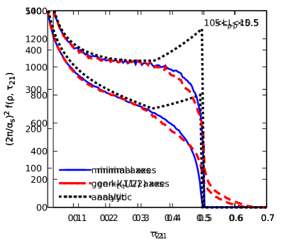
Figure 3: Comparison of our analytic results (dotted black) with the Event2 generator for the $\tau_{21}$ distribution in a bin of $\rho$. For the Event2 simulations, we show results for both the generalised-$k_{t}$ (solid red) and minimal axes (dashed blue). The left and right plots corresponds to different bins in $L_{\rho}=\log(1/\rho)$.

We first compare our results with a fixed-order calculation at the first order where a non-trivial $\tau$ dependence appears: ${\cal O}(\alpha_{s}^{2})$. In this case, we consider the distribution

$$H(\rho,>\tau)=H(\rho)-H(\rho,<\tau),$$ (43)

for a jet to have a given “mass” $\rho$ and a $\tau_{21}$ ratio be above a cut $\tau$. We do this as in this case we are sensitive to the situation with two real emission in the jet. To compute in our approximation Eq. 43, we expand Eq. (35) to order $\alpha_{s}^{2}$, which gives

$$H(\rho,>\tau)=R^{\prime}(\rho)\,[R(\rho\tilde{\tau})-R(\rho)]\,\Theta\big{(}\tau<\tfrac{1}{2}\big{)}.$$ (44)

We can then proceed by expanding $R$ and $R^{\prime}$ in $\alpha_{s}$ (equivalent to using a fixed-order prescription), which gives the leading logarithmic contribution in $\rho$.

$$H_{\text{plain}}(\rho,>\tau) =\Big{(}\frac{\alpha_{s}C_{F}}{\pi}\Big{)}^{2}\log\Big{(}\frac{1-\tau}{\tau}\Big{)}\log^{2}(\rho)+{\cal O}(\log(\rho)),$$ (45)

$$H_{\text{SD}}(\rho,>\tau) =\Big{(}\frac{\beta}{2+\beta}\frac{\alpha_{s}C_{F}}{\pi}\Big{)}^{2}\log\Big{(}\frac{1-\tau}{\tau}\Big{)}\log^{2}(\rho)+{\cal O}(\log(\rho)),$$ (46)

respectively for the plain jet and for a SoftDropped jet. Additionally, we take the derivative of Eq. (35) with respect to $\tau_{21}$, and perform a similar expansion, yielding the leading $\log(\rho)$ contribution as well as the double logarithmic term in $\tau_{21}$

$$f_{\text{plain}}(\rho,\tau_{21})=\Big{(}\frac{\alpha_{s}C_{F}}{\pi}\Big{)}^{2} \frac{1}{1-\tau}\Big{(}\log\Big{(}\frac{1}{\rho}\Big{)}+B_{q}\Big{)}$$ (47)

$$\times\bigg{[}\Big{(}\log\Big{(}\frac{1}{\rho}\Big{)}+\log\Big{(}\frac{1-\tau}{\tau}\Big{)}+B_{q}\Big{)}+\frac{C_{A}}{C_{F}}\Big{(}\log\Big{(}\frac{1-\tau}{\tau}\Big{)}+B_{g}\Big{)}\bigg{]}.$$

Note that we do not include in this case the similarly derived expressions in the SoftDrop jet case, as they are more lengthy and complex due to the constraint (39.

To check our accuracy claim, we test to what extent our approximations, Eqs (45) and (47), can reproduce a fixed-order prediction for the same observable. For this purpose, we use the Event2 Catani:1996jh ; Catani:1996vz generator, by rotating events to align them along one of the axis and proceed as if they were $pp$ collisions.

Additionally, to simulate the leading behaviour we are interested in, we compute the same quantities by integrating the triple collinear splitting function Campbell:1997hg ; Catani:1998nv ; Catani:1999ss without imposing any ordering or soft approximation. In small-$R$ limit this has the same $\alpha_{s}^{2}\log^{2}(\rho)$ and $\alpha_{s}^{2}\log(\rho)$ logarithmic dependence as an exact fixed-order calculation, for the plain jet (see also Sec. 3.2 of Dasgupta:2018emf ). This validity extends to larger $R$ in the SoftDrop case, which keeps only emissions at angles that are suppressed by powers of $\rho$. The high level of agreement between the two can be seen in the results presented in this section. We present this approximation too as it can be more easily pushed numerically to smaller values of $\rho$ and $\tau$, which one is interested in, and it might be easier to use in the case of matching to fixed-order.

We start by showing the $\tau_{21}$ distribution in Fig. 3. At small $\tau_{21}$ ($\tau_{21}\lesssim 0.3$) our analytic results are in perfect agreement with the exact Event2 results. For larger $\tau_{21}$, we see a transition at $\tau_{21}=\tfrac{1}{2}$, as already discussed in Sec. 4.1. Although this transition is present in the Event2 simulations as well, it appears to be smoother. Around the transition point, we also see some differences between the two choices of axes as well as a shoulder in the analytic calculation which is absent in the Event2 simulations. Increasing $\log(1/\rho)$, makes the transition at $\tau_{21}=\tfrac{1}{2}$ in Event 2 become sharper. This is expected, as for large $\log(1/\rho)$ our calculation captures the dominant $\alpha_{s}^{2}\log^{2}(1/\rho)$ contribution to $f(\rho,\tau)$, leaving corrections of order $\alpha_{s}^{2}\log(1/\rho)$. However this does not obviously seem the case in the shoulder region where the difference between Event2 and our analytic results seems to increase as rapidly as the rest of the distribution. We traced back this shoulder effect to differences between the exact $\tau_{21}$ and our leading-logarithmic approximation, Eq. (18), specifically in the region of similar angles ($\theta_{2}\sim\theta_{1}$ in Fig. 1). We discuss this in more details in Appendix C where we show that this region indeed only gives subleading corrections and that these corrections are increasingly numerically relevant when approaching $\tau_{21}=\tfrac{1}{2}$.

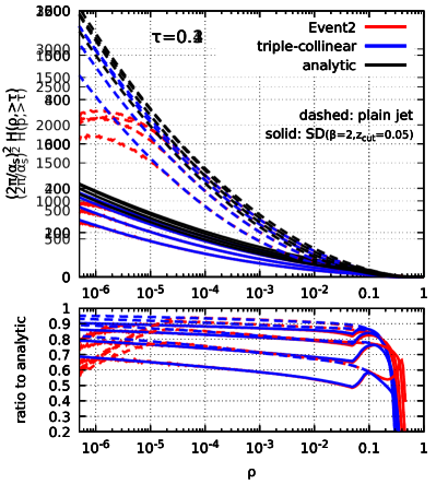
Figure 4: Comparison of our analytic results with the Event2 generator and with the triple-collinear splitting function for the $H(\rho,>\tau)$ distribution. Dashed and solid lines respectively correspond to results obtained using plain and SoftDropped jets. The top panel shows $H(\rho,>\tau)$ and the bottom panel shows the ratio to our analytic results. The left and right plots correspond to a cut $\tau=0.1$ and $\tau=0.3$, respectively.

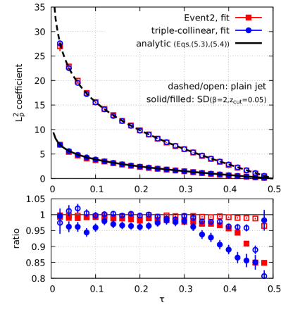
Figure 5: Coefficient of the $\log^{2}(1/\rho)$ contribution to the $H(\rho,>\tau)$ distribution. For the Event2 results (filled symbols) and the results obtained by integrating over the triple-collinear splitting function (open symbols), we perform a fit to the numerical results for each value of $\tau$. (Red) circles correspond to results obtained from the plain jet, and (black) squares to results where SoftDrop has first been applied. The plot insert shows the ratio to the expected analytic result.

A comparison of the $H(\rho,>\tau)$ distribution, obtained either from Event2 or integrating over the triple-collinear splitting function, to our analytic results is presented on Fig. 4. We plot $H(\rho,>\tau)$ as a function of $\rho$ for two different values of the $\tau$ cut. Results are shown for both the plain jet and SoftDropped jet (using $\beta=2$ and $z_{\text{cut}}=0.05$). As it can be seen, our calculation indeed captures the dominant $\log^{2}(1/\rho)$ behaviour. This is confirmed by Fig. 5 which shows the result for the coefficient of the leading $\log^{2}(1/\rho)$ contribution. For the Event2 and the triple-collinear results, we extract this coefficient using a simple fit of the distribution, for each individual cut on $\tau$. The fitted coefficient lies very closely to the expected analytic results, for both the plain and SoftDropped jets. We believe that the small discrepancy is related to the limited fitting range and the difficulty to obtain numerical results in the very small $\rho$ limit.

We also see in Fig. 4 that the triple-collinear results are almost identical to what is obtained from Event2, except in the large $\rho$ region where the triple-collinear approximation breaks down, and in the small $\rho$ region, where Event2 has an infrared cut-off causing the drop seen in the figure.

5.2 Parton shower Monte Carlo simulations

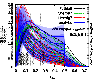
Figure 6: Differential distribution in $\tau$ compared to Monte Carlo for 3 different bins in $L_{\rho}=\log(1/\rho)$. We show our analytic results (with their uncertainty band) compared to the Pythia8, Sherpa2 and Herwig7 generators. All results are for jets groomed with SoftDrop. The vertical dashed lines indicate when the scale $\rho\tau$ starts to hit a given $k_{t}$ value, indicative of where non-perturbative effects are expected to become dominant.

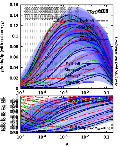
Figure 7: Mass distribution with a cut on $\tau_{21}$ compared to Monte Carlo for 3 different values of the cut. We show our analytic results (with their uncertainty band) compared to the Pythia8, Sherpa2 and Herwig7 generators. All results are for jets groomed with SoftDrop. The vertical dashed lines indicate when the scale $\rho\tau$ starts to hit a given $k_{t}$ value, indicative of where non-perturbative effects are expected to become dominant.

Setup.

We now compare our analytic result to parton shower Monte Carlo generators. For this, we simulate dijet events with three different generators: Pythia 8.230 Sjostrand:2014zea (Monash13 tune Skands:2014pea ), Sherpa 2.2.4 Gleisberg:2008ta and Herwig 7.1.1 Corcella:2002jc ; Bellm:2017bvx with angular-ordered shower. We only consider underlying fixed order matrix elements with quarks in the final states, which means that we can assume quark jets for our analytic results as well. Events are simulated at $\sqrt{s}=13$ TeV and we focus for the moment on parton level results. We reconstruct jets with the anti-$k_{t}$  algorithm Cacciari:2008gp with $R=1$ using FastJet 3.3.1 Cacciari:2005hq ; Cacciari:2011ma . We further require that all jets have $p_{t}>3$ TeV. We apply SoftDrop, using $\beta=2$ and $z_{\text{cut}}=0.05$, to each jet and compute the jet mass and $N$-subjettiness on the SoftDropped jet. For $\tau_{1}$ and $\tau_{2}$ we use the generalised-$k_{t}$($p=1/2$) (difference wrt to minimal axes in this case are smaller than what we observe with Event2). We then consider two distributions: either the $\tau_{21}$ distribution for jets within a restricted window of mass, or the jet mass distribution for a given cut on $\tau_{21}$. All analytical results shown here are obtained from the cumulative distribution computed in Sec. 4.3 (by taking the $\tau$ derivative to get the $\tau_{21}$ differential distribution), applied to SoftDropped jets (see Sec. 4.4), with the uncertainty band calculated as described in Sec. 4.5. For the radiators, we use the expressions reported in Appendix A, including running-coupling effects.

Comparison at parton level.

Our results for the $N$-subjettiness distribution are presented in Fig. 6 for three different bins in $L_{\rho}=\log(1/\rho)$. Overall, we see a good agreement between the Monte Carlo simulations and our approximation, already at relatively small values of $\log(1/\rho)$, with Herwig lying at the edge of our uncertainty band. As discussed in the previous sections, we expect and observe a transition at $\tau=\tfrac{1}{2}$ in the analytic calculation, which is smeared in Monte Carlo simulations. This can be explained by the fact they compute the value of $\tau_{21}$ exactly. Going above $\tau=\tfrac{1}{2}$, we observe, from our analytic calculation, a sizeable contribution due to multiple emissions. The dashed vertical lines on Fig. 6 indicate where our calculation becomes sensitive to a given $k_{t}$ scale (with the soft scale of our calculation taken as the lowest $k_{t}$ accessible for a mass scale of $\rho\tau$). As $k_{t}$ decreases, we expect sizeable non-perturbative contributions and we discuss this further in the following paragraph.

Fig. 7 shows the mass distribution obtained for three different cuts on $\tau_{21}$. The top panels show the raw mass distribution,while the bottom panels show the distribution normalised by the uncut mass distribution, highlighting the effect of the $N$-subjettiness cut itself. As expected, putting a tighter cut on $N$-subjettiness reduces the mass distribution. As before, we see a good agreement between our calculation and the Monte Carlo simulations, at least in the perturbative region. We also see differences between the three generators of the order of our estimated theory uncertainty.

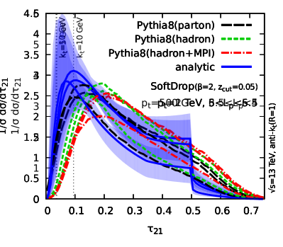
Figure 8: Same as Fig. 6 now for different values of $p_{t}$. Here we show results for the Pythia8 generator at different levels in order to gauge the importance of non-perturbative effects. For each $p_{t}$, the bin in $L_{\rho}=\log(1/\rho)$ is adjusted to be roughly around the mass of the $W$ boson (for definiteness).

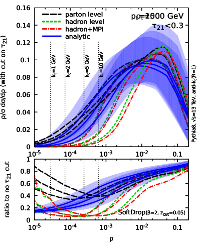
Figure 9: Same as Fig. 7 now for different values of $p_{t}$. Here we show results for the Pythia8 generator at different levels in order to gauge the importance of non-perturbative effects. All the plots use a representative cut on $\tau_{21}$ of 0.3.

Lower $p_{t}$ and non-perturbative effects.

We now want to check the level of agreement of our prediction when the jet $p_{t}$ is smaller and assess the importance of non-perturbative corrections. This is shown in Figs. 8 and 9, where the different plots correspond to $p_{t}$ cuts of 2 TeV, 1 TeV and 500 GeV respectively. For each $p_{t}$ we have adjusted the bin in $L_{\rho}=\log(1/\rho)$ to be roughly around the value of the $W$ mass, a typical scale where the $\tau_{21}$ ratio is used in phenomenological applications. We show in these plots Pythia distributions obtained from different type of events: parton level (long-dashed black lines), and hadron level with both multiple-parton-interactions (MPI) switched off (short-dashed green lines) and with MPI switch on (dash-dotted red lines). As far as the perturbative aspects are concerned, the agreement between our calculation and Pythia remains valid for smaller boosts. We see that hadronisation corrections have a sizeable impact on the distributions, even in regions of phase-space, where we are only sensitive to fairly large $k_{t}$ scales. Furthermore, while MPI effects are small for 1 and 2 TeV jets, they are sizeable for 500 GeV jets. These effects can be reduced by using a more aggressive grooming procedure, like a smaller value of $\beta$, e.g. using the modified MassDrop tagger (mMDT), or a larger value of $z_{\text{cut}}$. In that context, note that we have checked that our analytic calculations still work in the case of the mMDT where logarithms of $\rho$ resummed in our multiple-emission contributions (the $R^{\prime}(\rho\tau)$ factors) are now replaced by logarithms of $z_{\text{cut}}$.

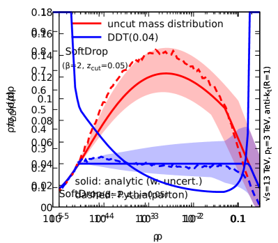
Figure 10: Analytic construction of a decorrelated tagger (DDT). Left: cut on $\tau_{21}$ which would give an analytic mass spectrum $\rho/\sigma d\sigma/d\rho=0.04$. Right: resulting mass spectrum analytically (with an uncertainty band) and using Pythia8.

Decorrelated taggers.

One interesting application of our analytic control of $N$-subjettiness cut is that it largely facilitates the design of a decorrelated tagger Dolen:2016kst : for each value of the mass, one can determine, based on our calculation, the value of the $\tau$ cut required to get a flat mass distribution at a given level, say, with $\rho/\sigma d\sigma/d\rho$ somewhere in the 0.03-0.04 range (lower values would start having a larger sensitivity to non-perturbative effects). We present the result of such a study in Fig. 10. For each value of $\rho$, we adjust the cut on $\tau_{21}$ so as to obtain $\rho/\sigma d\sigma/d\rho=0.04$. The cut one obtains is shown in the left plot (whenever the uncut distribution was already smaller than 0.04, we did not impose a further constraint on $\tau_{21}$). The resulting distribution is shown in the right plot together with an uncertainty band and the result of applying the same $\rho$-dependent $\tau_{21}$ cut on a (parton-level) Pythia simulation. We see that the resulting decorrelated distribution (labelled “DDT”) on the plot, in the Pythia simulation is almost flat, and at least within our analytic uncertainty. From a further study, one could conceive making a combined adjustment of the $\tau$ cut together with the SoftDrop parameters in order to obtain a flat background and maximise the signal efficiency for a colourless 2-body decay like in the case of electroweak ($H/W/Z$) bosons.

6 Conclusions

In perturbative QCD, boosted jets are characterised by large logarithms of $m/p_{t}$, i.e. the ratio of their mass to their transverse momentum. In this work we have shown how one can achieve an all-order resummation of the dominant logarithms of the jet mass in the presence of a cut on a jet shape. Compared to our previous work, we lift the assumption that the cut is small. This, in practice, allows one to take cut values of physical relevance. In this paper, we have focused on applying a cut on a particular jet shape, namely the $N$-subjettiness $\tau_{21}$ ratio with the angular exponent $\beta$ set to 2. We compute both the $\tau_{21}$ distribution for a boosted jet, and the jet mass distribution in the presence of a cut on $\tau_{21}$. The calculation is structured so as to also include the leading logarithms of the jet shape when it becomes small, hence recovering results from previous works.

Besides the analytic results presented throughout the paper for $\tau_{21}$, we are confident that the method can be applied to a wide range of other jet shapes. In a nutshell, the calculation is organised in a number of key steps: (i) starting from a generic sum over any number of real emissions, isolate the emission the dominates the jet mass, (ii) use the shape to deduce the relevant physical scale for the remaining emissions, (iii) simplify the expressions using CAESAR-like techniques, standard in resummation calculations. For more complex observables, one likely also have to isolate other dominant emissions in step (i), like the emission dominating the plain jet mass (potentially different from the one dominating the groomed jet mass) in the case of a dichroic $N$-subjettiness ratio, or the emission dominating the jet broadening (potentially different from the one dominating the jet mass) in the case of the $\beta=1$ $\tau_{21}$ ratio. The generic approach presented here is then expected to still apply. In the future, we plan to explore other jet shapes like $\tau_{21}$ ratios for a generic $\beta$, dichroic ratios Salam:2016yht and energy-correlation functions Larkoski:2013eya , as well as investigating shapes relevant for (3-prong) top tagging like the $\tau_{32}$ ratio. Concerning energy correlation functions, it would be interesting to compare our findings with results obtained in SCET e.g. for $D_{2}$ Larkoski:2015kga ; Larkoski:2017cqq ; Moult:2017okx , especially since $D_{2}$ appears to yield an efficient tagger (see e.g.  Bendavid:2018nar ).

We have compared our analytic predictions to the three most used Monte Carlo event generators, Pythia, Herwig and Sherpa, in two cases: the $\tau_{21}$ distribution and the jet mass distribution with a $\tau_{21}$ cut. We have concentrated on the case of jets previously groomed with SoftDrop, to limit non-perturbative effects. In both cases, we see a good agreement with Monte Carlo predictions, within our theoretical uncertainty band, in the region where resummation matters. As another example of a phenomenologically-relevant application of our results, we have used our analytic calculations to build a decorrelated tagger.

This work opens on several possible future developments. First, one could try to extend the precision of our calculation to include subleading logarithms and match it with fixed-order results. (Note however that reaching an NLO accuracy for the fixed-order part of the calculation would require $2\to 4$ QCD events at NLO.) Such a prediction could then be compared to an experimental measurement, similarly to what has been done recently for the groomed jet mass CMS:2017tdn ; Marzani:2017kqd ; Marzani:2017mva ; Aaboud:2017qwh . Finally, the theoretical uncertainty on our calculations, complemented with an assessment of the non-perturbative uncertainties, could then be used to estimate the theoretical uncertainty of boosted taggers used in searches.

Appendix A Explicit results for the radiators

The full expressions for the radiators and their derivatives are already available from the literature (see e.g.  Marzani:2017kqd ; Dasgupta:2015lxh ; Banfi:2004yd ). We summarise them here for completeness.

The SoftDrop radiator can be written as (assuming $\rho<z_{\text{cut}}$)

$$R_{\text{SD}}(\rho)=$$ (48)

$$=\frac{C_{i}}{2\pi\alpha_{s}\beta_{0}^{2}}\bigg{\{}\bigg{[}W(1-\lambda_{B})-\frac{W(1-\lambda_{c})}{1+\beta}-2W\Big{(}1-\frac{\lambda_{\rho}+\lambda_{B}}{2}\Big{)}+\frac{2+\beta}{1+\beta}W\Big{(}1-\frac{\lambda_{c}+(1+\beta)\lambda_{\rho}}{2+\beta}\Big{)}\bigg{]}$$

$$+\frac{\alpha_{s}\beta_{1}}{\beta_{0}}\bigg{[}V(1-\lambda_{B})-\frac{V(1-\lambda_{c})}{1+\beta}-2V\Big{(}1-\frac{\lambda_{\rho}+\lambda_{B}}{2}\Big{)}+\frac{2+\beta}{1+\beta}V\Big{(}1-\frac{\lambda_{c}+(1+\beta)\lambda_{\rho}}{2+\beta}\Big{)}\bigg{]}$$

$$-\frac{\alpha_{s}K}{2\pi}\bigg{[}\log(1-\lambda_{B})-\frac{\log(1-\lambda_{c})}{1+\beta}-2\log\Big{(}1-\frac{\lambda_{\rho}+\lambda_{B}}{2}\Big{)}+\frac{2+\beta}{1+\beta}\log\Big{(}1-\frac{\lambda_{c}+(1+\beta)\lambda_{\rho}}{2+\beta}\Big{)}\bigg{]}\bigg{\}}\,,$$

where $\lambda_{\rho}=2\alpha_{s}\beta_{0}\log(\tfrac{1}{\rho})$, $\lambda_{c}=2\alpha_{s}\beta_{0}\log(\tfrac{1}{z_{\text{cut}}})$ and $\lambda_{B}=-2\alpha_{s}\beta_{0}B_{i}$ (associated with hard-collinear splittings). and $W(x)=x\log(x)$, $V(x)=\tfrac{1}{2}\log^{2}(x)+\log(x)$. The expression above is computed using a two-loop running coupling in the CMW scheme Catani:1990rr , and $\alpha_{s}$ is taken at the hard scale $p_{t}R$. The results for $R^{\prime}$ can be straightforwardly obtained by taking a derivative of the above expression wrt $\log(\tfrac{1}{\rho})$ and the plain jet radiators are obtained by taking either $\beta$ to $\infty$ or $z_{\text{cut}}$ to $0$.

For $R_{\text{SD}}(\rho\tilde{\tau};z_{a})$, Eq. (41), we need two further ingredients: the possible extra contribution from $\theta>\theta_{a}$ (and $z<z_{\text{cut}}\theta^{\beta}$, since the rest is already included in the expression above), and the contribution from secondary emissions. Introducing

$$\delta R_{\beta}(\lambda_{\text{top}},\lambda_{\text{bot}})=\frac{C_{i}}{2\pi\alpha_{s}\beta_{0}^{2}}\bigg{\{}\bigg{[}\frac{W(1-\lambda_{\text{top}})}{1+\beta}+W(1-\lambda_{\text{bot}})-\frac{2+\beta}{1+\beta}W\Big{(}1-\frac{\lambda_{\text{top}}+(1+\beta)\lambda_{\text{bot}}}{2+\beta}\Big{)}\bigg{]}$$

$$\quad+\frac{\alpha_{s}\beta_{1}}{\beta_{0}}\bigg{[}\frac{V(1-\lambda_{\text{top}})}{1+\beta}+V(1-\lambda_{\text{bot}})-\frac{2+\beta}{1+\beta}W\Big{(}1-\frac{\lambda_{\text{top}}+(1+\beta)\lambda_{\text{bot}}}{2+\beta}\Big{)}\bigg{]}$$

$$\quad-\frac{\alpha_{s}K}{2\pi}\bigg{[}\frac{\log(1-\lambda_{\text{top}})}{1+\beta}+\log(1-\lambda_{\text{bot}})-\frac{2+\beta}{1+\beta}\log\Big{(}1-\frac{\lambda_{\text{top}}+(1+\beta)\lambda_{\text{bot}}}{2+\beta}\Big{)}\bigg{]}\bigg{\}}\,\Theta(\lambda_{\text{bot}}>\lambda_{\text{top}})\,,$$

x we can write the “extra triangle” and secondary contributions as

$$R_{\text{SD,extra}}(\rho\tau,z_{a}) =\delta R_{\beta}\Big{(}\lambda_{c}+(\beta+1)\frac{\lambda_{\rho}-\lambda_{a}}{2},\frac{\lambda_{\rho}-\lambda_{a}}{2}+\lambda_{\tau}\Big{)},$$ (49)

$$R_{\text{secondary}}(\rho\tau,z_{a}) =\delta R_{\beta}\Big{(}\frac{\lambda_{\rho}+\lambda_{a}}{2},\frac{\lambda_{\rho}+\lambda_{a}}{2}+\lambda_{\tau}\Big{)},$$ (50)

with $\lambda_{\tau}=2\alpha_{s}\beta_{0}\log(1/\tau)$ and $\lambda_{a}=2\alpha_{s}\beta_{0}\log(1/z_{a})$.

Appendix B The multiple-emission function $f_{\text{ME}}$

In practice, $f_{\text{ME}}(x,R^{\prime})$ can be computed analytically for $x\leq 1$, and $1<x\leq 2$ and we have managed to reduce it to a single integration at least for $2<x\leq 4$:

$$f_{\text{ME}}(x,R^{\prime}) \mathrel{\mathop{\quad=\quad}\limits^{\vbox to3.41418pt{\kern-2.0pt\hbox{$\scriptstyle x\leq 1$}\vss}}}x^{R^{\prime}-1},$$ (51)

$$\mathrel{\mathop{\quad=\quad}\limits^{\vbox to3.41418pt{\kern-2.0pt\hbox{$\scriptstyle 1<x\leq 2$}\vss}}}x^{R^{\prime}-1}\bigg{[}1-\Big{(}\frac{x-1}{x}\Big{)}^{R^{\prime}}{}_{2}F_{1}\Big{(}R^{\prime},1,1+R^{\prime},\frac{x-1}{x}\Big{)}\bigg{]},$$

$$\mathrel{\mathop{\quad=\quad}\limits^{\vbox to3.41418pt{\kern-2.0pt\hbox{$\scriptstyle 2<x\leq 3$}\vss}}}f_{\text{ME}}(2,R^{\prime})+R^{\prime 2}\int_{0}^{x-2}du\,\frac{u^{R^{\prime}-1}}{x-u}\log(x-1-u),$$

$$\mathrel{\mathop{\quad=\quad}\limits^{\vbox to3.41418pt{\kern-2.0pt\hbox{$\scriptstyle 3<x\leq 4$}\vss}}}f_{\text{ME}}(3,R^{\prime})+R^{\prime 3}\int_{0}^{x-3}du\,\frac{u^{R^{\prime}-1}}{x-u}\Big{[}\text{Li}_{2}\Big{(}\frac{1}{x-1-u}\Big{)}+\frac{1}{2}\log^{2}(x-1-u)-\frac{\pi^{2}}{12}\Big{]}$$

In general, we write $f_{\text{ME}}(x,R^{\prime})$ as an inverse Mellin transform, which is what we have used for $x>4$:

$$f_{\text{ME}}(x,R^{\prime})=\Gamma(R^{\prime})\oint\frac{d\nu}{2i\pi}e^{\nu x}\exp\bigg{\{}\frac{R^{\prime}}{2}\text{Ei}(-\nu)\bigg{[}\log(-\nu)-\log\bigg{(}\!\!-\frac{1}{\nu}\bigg{)}\bigg{]}\bigg{\}}.$$ (52)

Appendix C Subleading contributions from similar angles

In this Appendix, we investigate the difference between the ${\cal{O}}(\alpha_{s}^{2})$ fixed-order predictions and our analytic expressions for the $\tau_{21}$ distribution in the shoulder region, $\tau_{21}\lesssim\tfrac{1}{2}$, and trace it back to a subleading contribution in the region where two emissions have similar angles. To show this, we work at small jet radius and use the framework of the integration over the triple-collinear splitting function. At ${\cal{O}}(\alpha_{s}^{2})$, a jet is made of 3 partons of momentum fractions $z_{i}$ and pairwise angles $\theta_{ij}$ with $i,j=1,2,3$, constrained so that $z_{1}z_{2}\theta_{12}^{2}+z_{1}z_{3}\theta_{13}^{2}+z_{2}z_{3}\theta_{23}^{2}=\rho$. For simplicity, we focus on the $C_{F}^{2}$ term, as the other contributions are subleading in $\log(\rho)$. We can then assume that particles 1 and 2 are gluons and particle 3 is a quark.

The expression for $\tau_{2}$ for the minimal axes can be obtained by minimising over all possible partitions of the jet and can be written as

$$\tau_{2}^{\text{(min)}}=\text{min}\Big{(}\frac{z_{1}z_{2}}{z_{1}+z_{2}}\theta_{12}^{2},\frac{z_{1}z_{3}}{z_{1}+z_{3}}\theta_{13}^{2},\frac{z_{2}z_{3}}{z_{2}+z_{3}}\theta_{23}^{2}\Big{)}\qquad\qquad\text{[minimal]}.$$ (53)

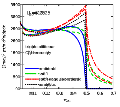
Figure 11: $\tau_{21}$ distributions at ${\cal{O}}(\alpha_{s}^{2})$ in the triple-collinear limit, obtained with different approximations for $\tau_{2}$. See text for details.

Our leading-logarithmic expression, Eq. (18), is obtained from $\tau_{2}^{\text{(min)}}$ by applying two approximations. Firstly, logarithms of $\rho$ come from soft emissions, $z_{1,2}\ll 1$, $z_{3}\approx 1$, yielding

$$\tau_{2}^{\text{(soft)}}=\text{min}\Big{(}\frac{z_{1}z_{2}}{z_{1}+z_{2}}\theta_{12}^{2},z_{1}\theta_{13}^{2},z_{2}\theta_{23}^{2}\Big{)}\qquad\qquad\text{[soft]},$$ (54)

with $\theta_{13}\approx\theta_{1}$ and $\theta_{23}\approx\theta_{2}$. Secondly, if each emission comes with a logarithm of $\rho$, they can be taken as strongly ordered in angles meaning $\frac{z_{1}z_{2}}{z_{1}+z_{2}}\theta_{12}^{2}\approx\text{max}(z_{1}\theta_{1}^{2},z_{2}\theta_{2}^{2})$ and therefore

$$\tau_{2}^{\text{(soft+ang.-ordered)}}=\text{min}\Big{(}z_{1}\theta_{13}^{2},z_{2}\theta_{23}^{2}\Big{)}\qquad\qquad\text{[soft+ang.-ordered]},$$ (55)

which is to all practical purposes the expression (18) we use throughout this paper.

In Fig. 11, we plot results obtained by integrating the triple-collinear splitting function for the plain jet, with $\tau_{21}$ computed using the three definitions above, and compare the results with our analytical formula. The striking feature here is that the above approximations mostly affect the region close to $\tau_{21}=\tfrac{1}{2}$, meaning that subleading logarithmic corrections are expected to have a non-negligible impact in this region for reasonable values of $\log(1/\rho)$.

It is helpful to discuss in a bit more details the differences associated with the soft and angular-ordered approximations. For the soft approximation, we see in Fig. 1 (right) that the correction indeed only affect a region of finite width at large $z_{2}$. This therefore gives at most a constant upon integration over $z_{2}$, subleading compared to the $\log(1/\rho)$ one would obtain from the integration in the soft limit. Interestingly, the difference between the minimal axes and the soft approximation appears mostly in the region above $\tau_{21}=\tfrac{1}{2}$, where we also see differences between the minimal and generalised-$k_{t}$ choices of axes. Although we have not explicitly checked that, the value of $\tau_{21}$ generalised-$k_{t}$ is likely affected by factors of $1-z$ in that region, due to differences between a pairwise mass $z_{i}z_{j}\theta_{ij}^{2}$ and the generalised-$k_{t}$ distance $\text{min}(z_{i},z_{j})\theta_{ij}^{2}$.

Next, we want to show explicitly that the contribution coming from emissions of similar angles, i.e. using $\tau_{2}^{\text{(soft)}}$ instead of $\tau_{2}^{\text{(soft+ang.-ordered)}}$, also leads to a subleading correction. This is particularly interesting because, from Fig. 11, it appears to be the main contribution driving the shoulder effect for $\tau_{21}\lesssim\tfrac{1}{2}$. For simplicity, let us consider the case of the cumulative distribution $H(\rho,>\tau)$ with two emissions “1” and “2”, and look at the contribution coming from the integration over emission “2”, with $\rho_{2}<\rho_{1}$ for a fixed $\rho$ and $\theta_{1}$. This can be written as

$$I_{2}=\int_{0}^{\rho/2}\frac{\rho\,d\rho_{2}}{\rho_{2}(\rho-\rho_{2})}\int_{\rho_{2}}^{1}\frac{d\theta_{2}^{2}}{\theta_{2}^{2}}\int_{0}^{2\pi}\frac{d\phi}{2\pi}\Theta\Big{(}\text{min}\Big{(}\frac{z_{1}z_{2}}{z_{1}+z_{2}}\theta_{12}^{2},\rho_{2}\Big{)}>\rho\tau\Big{)},$$ (56)

where we use the soft approximation, Eq. (54), and $\theta_{12}^{2}=\theta_{1}^{2}-2\theta_{1}\theta_{2}\cos\phi+\theta_{2}^{2}$. We can write $I_{2}$ as a “leading” contribution coming from the approximation in (55) and a correction:

$$I_{2} =I_{2,\text{leading}}-\delta I_{2},$$ (57)

$$I_{2,\text{leading}} =\int_{0}^{\rho/2}\frac{\rho\,d\rho_{2}}{\rho_{2}(\rho-\rho_{2})}\int_{\rho_{2}}^{1}\frac{d\theta_{2}^{2}}{\theta_{2}^{2}}\int_{0}^{2\pi}\frac{d\phi}{2\pi}\Theta(\rho_{2}>\rho\tau)=\log\Big{(}\frac{1-\tau}{\tau}\Big{)}\log\Big{(}\frac{1}{\rho}\Big{)}+\text{const.},$$ (58)

$$\delta I_{2} =\int_{0}^{\rho/2}\frac{\rho\,d\rho_{2}}{\rho_{2}(\rho-\rho_{2})}\int_{\rho_{2}}^{1}\frac{d\theta_{2}^{2}}{\theta_{2}^{2}}\int_{0}^{2\pi}\frac{d\phi}{2\pi}\Theta\Big{(}\text{min}\Big{(}\frac{z_{1}z_{2}}{z_{1}+z_{2}}\theta_{12}^{2},\rho_{2}\Big{)}<\rho\tau<\rho_{2}\Big{)}.$$ (59)

Here, $I_{2,\text{leading}}$ is the leading contribution we compute to all orders in this paper and $\delta I_{2}$ is a correction. We want to show that $\delta I_{2}$ is subleading, i.e. that it does not come with any $\log(\rho)$ enhancement. For that it is sufficient to show that the integration over $\theta_{2}$, which is at the origin of the $\log(1/\rho)$ in $I_{2,\text{leading}}$, now contributes at most to a constant in $\rho$. For the constraint in (59) to be non-zero, we need $\tfrac{z_{1}z_{2}}{z_{1}+z_{2}}\theta_{12}^{2}<\rho_{2}$ and $\cos(\phi)<1$ from which we get $\tfrac{\theta_{2}}{\theta_{1}}>\tfrac{\rho-2\rho_{2}}{2(\rho-\rho_{2})}$. Since the right hand side is a number, the limit of small $\theta_{2}$ does not give a large logarithm of $\rho$.

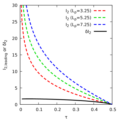
Figure 12: Contribution of the subleading $\delta I_{2}$ contribution, compared to the leading $I_{2,\text{leading}}$ contribution for different values of $L_{\rho}=\log(1/\rho)$.

In the limit of large $\theta_{2}$, we can rewrite the constraint as $\tau<\tfrac{\rho_{2}}{\rho}<\tau(1+2\tfrac{\theta_{1}}{\theta_{2}}\cos\phi+{\cal{O}}(\tfrac{\theta_{1}^{2}}{\theta_{2}^{2}}))$. The integration over $\rho_{2}$ therefore brings an extra factor $\tfrac{\theta_{1}}{\theta_{2}}$ suppressing the large-$\theta_{2}$ contribution. This corresponds to the decrease towards a ratio of 1 at large $\theta_{2}$ in Fig. 1. Altogether, this implies that $\delta I_{2}$ does not have any $\log(1/\rho)$ enhancement. To further illustrate this point, we plot $\delta I_{2}$ in Fig. 12, compared to the leading contribution $I_{2,\text{leading}}$. We obtain this by numerically integrating Eqs. (58), setting the limits of the $\theta_{2}$ integration to $\pm\infty$ so that it becomes independent of $\rho$, and keeping only the leading $\log(\rho)$ contribution in $I_{2,\text{leading}}$. We clearly see on this plot that the $\delta I_{2}$ contribution has a relatively larger impact as $\tau$ increases.

References

- (1) A. J. Larkoski, I. Moult, and B. Nachman, Jet Substructure at the Large Hadron Collider: A Review of Recent Advances in Theory and Machine Learning, arXiv:1709.04464.
- (2) L. Asquith et al., Jet Substructure at the Large Hadron Collider : Experimental Review, arXiv:1803.06991.
- (3) CMS Collaboration, A. M. Sirunyan et al., Search for vector-like T and B quark pairs in final states with leptons at 13 TeV, JHEP 08 (2018) 177, [arXiv:1805.04758].
- (4) CMS Collaboration, A. M. Sirunyan et al., Search for a new heavy resonance decaying into a Z boson and a Z or W boson in 22q final states at 13 TeV, arXiv:1803.10093.
- (5) CMS Collaboration, C. Collaboration, Search for a heavy resonance decaying into a vector boson and a Higgs boson in semileptonic final states at , .
- (6) ATLAS Collaboration, M. Aaboud et al., Search for decays in the hadronic final state using pp collisions at TeV with the ATLAS detector, Phys. Lett. B781 (2018) 327–348, [arXiv:1801.07893].
- (7) ATLAS Collaboration, M. Aaboud et al., Search for light resonances decaying to boosted quark pairs and produced in association with a photon or a jet in proton-proton collisions at TeV with the ATLAS detector, arXiv:1801.08769.
- (8) ATLAS Collaboration, M. Aaboud et al., Search for heavy particles decaying into top-quark pairs using lepton-plus-jets events in proton–proton collisions at TeV with the ATLAS detector, Eur. Phys. J. C78 (2018), no. 7 565, [arXiv:1804.10823].
- (9) CMS Collaboration, A. M. Sirunyan et al., Inclusive search for a highly boosted Higgs boson decaying to a bottom quark-antiquark pair, Phys. Rev. Lett. 120 (2018), no. 7 071802, [arXiv:1709.05543].
- (10) M. Dasgupta, A. Fregoso, S. Marzani, and G. P. Salam, Towards an understanding of jet substructure, JHEP 09 (2013) 029, [arXiv:1307.0007].
- (11) M. Dasgupta, A. Fregoso, S. Marzani, and A. Powling, Jet substructure with analytical methods, Eur. Phys. J. C73 (2013), no. 11 2623, [arXiv:1307.0013].
- (12) A. J. Larkoski, G. P. Salam, and J. Thaler, Energy Correlation Functions for Jet Substructure, JHEP 06 (2013) 108, [arXiv:1305.0007].
- (13) A. J. Larkoski, S. Marzani, G. Soyez, and J. Thaler, Soft Drop, JHEP 05 (2014) 146, [arXiv:1402.2657].
- (14) A. J. Larkoski, I. Moult, and D. Neill, Analytic Boosted Boson Discrimination, JHEP 05 (2016) 117, [arXiv:1507.03018].
- (15) M. Dasgupta, L. Schunk, and G. Soyez, Jet shapes for boosted jet two-prong decays from first-principles, JHEP 04 (2016) 166, [arXiv:1512.00516].
- (16) M. Dasgupta, A. Powling, L. Schunk, and G. Soyez, Improved jet substructure methods: Y-splitter and variants with grooming, JHEP 12 (2016) 079, [arXiv:1609.07149].
- (17) A. J. Larkoski, I. Moult, and D. Neill, Factorization and Resummation for Groomed Multi-Prong Jet Shapes, JHEP 02 (2018) 144, [arXiv:1710.00014].
- (18) I. Moult, B. Nachman, and D. Neill, Convolved Substructure: Analytically Decorrelating Jet Substructure Observables, JHEP 05 (2018) 002, [arXiv:1710.06859].
- (19) M. Dasgupta, M. Guzzi, J. Rawling, and G. Soyez, Top tagging : an analytical perspective, arXiv:1807.04767.
- (20) CMS Collaboration, A. M. Sirunyan et al., Measurement of the Splitting Function in and Pb-Pb Collisions at 5.02 TeV, Phys. Rev. Lett. 120 (2018), no. 14 142302, [arXiv:1708.09429].
- (21) ALICE Collaboration, D. Caffarri, Exploring jet substructure with jet shapes in ALICE, Nucl. Phys. A967 (2017) 528–531, [arXiv:1704.05230].
- (22) Y.-T. Chien and R. Kunnawalkam Elayavalli, Probing heavy ion collisions using quark and gluon jet substructure, arXiv:1803.03589.
- (23) ALICE Collaboration, H. Andrews, Exploring phase space of jet splittings at alice using grooming and recursive techniques, 2018. Talk at Quark Matter 2018, Venice, Italy, https://indico.cern.ch/event/656452/contributions/2869941/attachments/1649044/2636550/HarryAndrews_QuarkMatter18Final.pdf.
- (24) M. Connors, C. Nattrass, R. Reed, and S. Salur, Jet measurements in heavy ion physics, Rev. Mod. Phys. 90 (2018) 025005, [arXiv:1705.01974].
- (25) J. Cogan, M. Kagan, E. Strauss, and A. Schwarztman, Jet-Images: Computer Vision Inspired Techniques for Jet Tagging, JHEP 02 (2015) 118, [arXiv:1407.5675].
- (26) L. de Oliveira, M. Kagan, L. Mackey, B. Nachman, and A. Schwartzman, Jet-images — deep learning edition, JHEP 07 (2016) 069, [arXiv:1511.05190].
- (27) P. T. Komiske, E. M. Metodiev, and M. D. Schwartz, Deep learning in color: towards automated quark/gluon jet discrimination, JHEP 01 (2017) 110, [arXiv:1612.01551].
- (28) G. Kasieczka, T. Plehn, M. Russell, and T. Schell, Deep-learning Top Taggers or The End of QCD?, JHEP 05 (2017) 006, [arXiv:1701.08784].
- (29) G. Louppe, K. Cho, C. Becot, and K. Cranmer, QCD-Aware Recursive Neural Networks for Jet Physics, arXiv:1702.00748.
- (30) S. Egan, W. Fedorko, A. Lister, J. Pearkes, and C. Gay, Long Short-Term Memory (LSTM) networks with jet constituents for boosted top tagging at the LHC, arXiv:1711.09059.
- (31) A. Andreassen, I. Feige, C. Frye, and M. D. Schwartz, JUNIPR: a Framework for Unsupervised Machine Learning in Particle Physics, arXiv:1804.09720.
- (32) K. Datta and A. Larkoski, How Much Information is in a Jet?, JHEP 06 (2017) 073, [arXiv:1704.08249].
- (33) K. Datta and A. J. Larkoski, Novel Jet Observables from Machine Learning, JHEP 03 (2018) 086, [arXiv:1710.01305].
- (34) P. T. Komiske, E. M. Metodiev, and J. Thaler, Energy flow polynomials: A complete linear basis for jet substructure, JHEP 04 (2018) 013, [arXiv:1712.07124].
- (35) F. A. Dreyer, G. P. Salam, and G. Soyez, The Lund Jet Plane, arXiv:1807.04758.
- (36) CMS Collaboration, C. Collaboration, Measurement of the differential jet production cross section with respect to jet mass and transverse momentum in dijet events from pp collisions at = 13 TeV, .
- (37) ATLAS Collaboration, M. Aaboud et al., A measurement of the soft-drop jet mass in pp collisions at TeV with the ATLAS detector, Phys. Rev. Lett. 121 (2018), no. 9 092001, [arXiv:1711.08341].
- (38) S. Marzani, L. Schunk, and G. Soyez, A study of jet mass distributions with grooming, JHEP 07 (2017) 132, [arXiv:1704.02210].
- (39) S. Marzani, L. Schunk, and G. Soyez, The jet mass distribution after Soft Drop, Eur. Phys. J. C78 (2018), no. 2 96, [arXiv:1712.05105].
- (40) C. Frye, A. J. Larkoski, M. D. Schwartz, and K. Yan, Factorization for groomed jet substructure beyond the next-to-leading logarithm, JHEP 07 (2016) 064, [arXiv:1603.09338].
- (41) J. Thaler and K. Van Tilburg, Identifying Boosted Objects with N-subjettiness, JHEP 03 (2011) 015, [arXiv:1011.2268].
- (42) J.-H. Kim, Rest Frame Subjet Algorithm With SISCone Jet For Fully Hadronic Decaying Higgs Search, Phys. Rev. D83 (2011) 011502, [arXiv:1011.1493].
- (43) J. Thaler and K. Van Tilburg, Maximizing Boosted Top Identification by Minimizing N-subjettiness, JHEP 02 (2012) 093, [arXiv:1108.2701].
- (44) A. J. Larkoski, I. Moult, and D. Neill, Power Counting to Better Jet Observables, JHEP 12 (2014) 009, [arXiv:1409.6298].
- (45) G. P. Salam, L. Schunk, and G. Soyez, Dichroic subjettiness ratios to distinguish colour flows in boosted boson tagging, JHEP 03 (2017) 022, [arXiv:1612.03917].
- (46) J. Dolen, P. Harris, S. Marzani, S. Rappoccio, and N. Tran, Thinking outside the ROCs: Designing Decorrelated Taggers (DDT) for jet substructure, JHEP 05 (2016) 156, [arXiv:1603.00027].
- (47) J. R. Andersen et al., Les Houches 2017: Physics at TeV Colliders Standard Model Working Group Report, in 10th Les Houches Workshop on Physics at TeV Colliders (PhysTeV 2017) Les Houches, France, June 5-23, 2017, 2018. arXiv:1803.07977.
- (48) “Fastjet contrib.” https://fastjet.hepforge.org/contrib/.
- (49) A. Banfi, G. P. Salam, and G. Zanderighi, Principles of general final-state resummation and automated implementation, JHEP 03 (2005) 073, [hep-ph/0407286].
- (50) A. J. Larkoski, D. Neill, and J. Thaler, Jet Shapes with the Broadening Axis, JHEP 04 (2014) 017, [arXiv:1401.2158].
- (51) A. J. Larkoski and J. Thaler, Unsafe but Calculable: Ratios of Angularities in Perturbative QCD, JHEP 09 (2013) 137, [arXiv:1307.1699].
- (52) A. J. Larkoski, S. Marzani, and J. Thaler, Sudakov Safety in Perturbative QCD, Phys. Rev. D91 (2015), no. 11 111501, [arXiv:1502.01719].
- (53) S. Catani and M. H. Seymour, The Dipole formalism for the calculation of QCD jet cross-sections at next-to-leading o rder, Phys. Lett. B378 (1996) 287–301, [hep-ph/9602277].
- (54) S. Catani and M. H. Seymour, A General algorithm for calculating jet cross-sections in NLO QCD, Nucl. Phys. B485 (1997) 291–419, [hep-ph/9605323]. [Erratum: Nucl. Phys.B510,503(1998)].
- (55) J. M. Campbell and E. W. N. Glover, Double unresolved approximations to multiparton scattering amplitudes, Nucl. Phys. B527 (1998) 264–288, [hep-ph/9710255].
- (56) S. Catani and M. Grazzini, Collinear factorization and splitting functions for next-to-next-to-leading order QCD calculations, Phys. Lett. B446 (1999) 143–152, [hep-ph/9810389].
- (57) S. Catani and M. Grazzini, Infrared factorization of tree level QCD amplitudes at the next-to-next-to-leading order and beyond, Nucl. Phys. B570 (2000) 287–325, [hep-ph/9908523].
- (58) T. Sjöstrand, S. Ask, J. R. Christiansen, R. Corke, N. Desai, P. Ilten, S. Mrenna, S. Prestel, C. O. Rasmussen, and P. Z. Skands, An Introduction to PYTHIA 8.2, Comput. Phys. Commun. 191 (2015) 159–177, [arXiv:1410.3012].
- (59) P. Skands, S. Carrazza, and J. Rojo, Tuning PYTHIA 8.1: the Monash 2013 Tune, Eur. Phys. J. C74 (2014), no. 8 3024, [arXiv:1404.5630].
- (60) T. Gleisberg, S. Hoeche, F. Krauss, M. Schonherr, S. Schumann, F. Siegert, and J. Winter, Event generation with SHERPA 1.1, JHEP 02 (2009) 007, [arXiv:0811.4622].
- (61) G. Corcella, I. G. Knowles, G. Marchesini, S. Moretti, K. Odagiri, P. Richardson, M. H. Seymour, and B. R. Webber, HERWIG 6.5 release note, hep-ph/0210213.
- (62) J. Bellm et al., Herwig 7.1 Release Note, arXiv:1705.06919.
- (63) M. Cacciari, G. P. Salam, and G. Soyez, The Anti-k(t) jet clustering algorithm, JHEP 04 (2008) 063, [arXiv:0802.1189].
- (64) M. Cacciari and G. P. Salam, Dispelling the myth for the jet-finder, Phys. Lett. B641 (2006) 57–61, [hep-ph/0512210].
- (65) M. Cacciari, G. P. Salam, and G. Soyez, FastJet User Manual, Eur. Phys. J. C72 (2012) 1896, [arXiv:1111.6097].
- (66) S. Catani, B. R. Webber, and G. Marchesini, QCD coherent branching and semi-inclusive processes at large x, Nucl. Phys. B349 (1991) 635–654.