Simplicity Creates Inequity:
Implications for Fairness, Stereotypes, and Interpretability

Abstract

Algorithms are increasingly used to aid, or in some cases supplant, human decision-making, particularly for decisions that hinge on predictions. As a result, two additional features in addition to prediction quality have generated interest: (i) to facilitate human interaction and understanding with these algorithms, we desire prediction functions that are in some fashion simple or interpretable; and (ii) because they influence consequential decisions, we also want them to produce equitable allocations. We develop a formal model to explore the relationship between the demands of simplicity and equity. Although the two concepts appear to be motivated by qualitatively distinct goals, we show a fundamental inconsistency between them. Specifically, we formalize a general framework for producing simple prediction functions, and in this framework we establish two basic results. First, every simple prediction function is strictly improvable: there exists a more complex prediction function that is both strictly more efficient and also strictly more equitable. Put another way, using a simple prediction function both reduces utility for disadvantaged groups and reduces overall welfare relative to other options. Second, we show that simple prediction functions necessarily create incentives to use information about individuals’ membership in a disadvantaged group — incentives that weren’t present before simplification, and that work against these individuals. Thus, simplicity transforms disadvantage into bias against the disadvantaged group. Our results are not only about algorithms but about any process that produces simple models, and as such they connect to the psychology of stereotypes and to an earlier economics literature on statistical discrimination.

1 Introduction

Algorithms can be a powerful aid to decision-making — particularly when decisions rely, even implicitly, on predictions [23]. We are already seeing algorithms play this role in domains including hiring, education, lending, medicine, and criminal justice [8, 22, 34, 36]. Across these diverse contexts, the role for algorithms follows a similar template: applicants present themselves to be evaluated by a decision-maker who chooses an accept/reject outcome for each applicant — for example, whether they are hired, admitted to a selective school, offered a loan, or released on bail. The final decision-making authority in these situations typically rests with a human being or a committee of human beings. But because the decisions turn on a prediction of some underlying quantity (such as crime risk in the case of bail or default risk in the case of a loan), decision-makers are beginning to rely on the assistance of algorithms that map features of each applicant to a numerical prediction.

As is typical in machine learning applications, accuracy, evaluated by some measure of admitted applicants’ future performance, is an important measure. In these high-stakes policy contexts, though, two additional considerations prove important as well, as highlighted by recent work:

• Fairness and equity. Certain groups in society are disadvantaged in clear-cut quantitative ways — on average they graduate from less-resourced educational institutions, live in areas with reduced economic opportunities, and face other socioeconomic challenges in aggregate. Will an algorithmic approach, based on these underlying measures, perpetuate (or even magnify) the underlying disadvantage? Or could we use algorithms to increase equity between groups? [4, 9, 12, 14]

• Interpretability. Algorithms tend to result in complex models that are hard for human beings to comprehend. Yet in these domains, humans work intimately with them. Can a decision-maker derive understanding from such an algorithm’s output, or are they forced to treat it as a “black box” that produces pure numerical predictions with no accompanying insight? And similarly, can an applicant derive any understanding about the basis for the algorithm’s prediction in their particular case? [11, 28, 38]

Fairness and interpretability are clearly distinct issues, but it is natural to suspect that there may be certain interactions between them. A common theme in the literature on interpretability is the possibility that interpretable models can be more easily examined and audited for evidence of unfairness or bias; as one of many examples of this theme, Doshi-Velez and Kim argue that “interpretability can assist in qualitatively ascertaining whether other desiderata — such as fairness, privacy, reliability, robustness, causality, usability and trust — are met” [11]. Nor is this point purely an issue in academic research: the formulation of the European Union General Data Protection Regulation (GDPR) reinforces earlier EU regulations asserting that individuals have a “right to explanation” when they are affected by algorithmic decision-making. The technical implications of these guidelines are not yet fully clear, but their premise situates interpretable decisions as a component of fair outcomes [17, 28].

The present work: A basic tension between fairness and simplicity.

There are many ways in which interpretability may be able to help promote fairness — they might be more easily analyzable and auditable, as noted above; and the activity of constructing an interpretable rule, depending how it is carried out, may be able to engage more participants in the process.

But there has been arguably less exploration of what, if anything, we give up with respect to fairness and equity when we pursue interpretable rules. Here we consider a set of questions in this direction, focusing in particular on the role of simplicity in the construction of prediction rules. Simplification is one of the common strategies employed in the construction of interpretable models, and this is for natural reasons. A primary source of model complexity is “width” — the number of variables, or applicant features, that are used. Humans typically struggle to understand very wide models, and so to create interpretable or explainable models, many standard approaches seek, at some level, to reduce the number of variables that go into in any one decision. There are many ways to do this: for example, we could project the space of features onto a small number of the most informative variables; we could enumerate short “rules” that only depend on a few variables; we could construct a shallow decision tree that only consults a small number of variables on any path from its root to a leaf. Despite the diversity in these approaches, they follow a common principle: they all simplify the underlying model by combining distinguishable applicants into larger sets and making a common decision at the level of each set.

Our main results show that when one group of individuals is disadvantaged with respect to another, there is a precise sense in which the process of simplifying a model will necessarily hurt natural measures of fairness and equity.

The present work: Summary of results.

The exact statement of our results will be made precise via the model that we develop starting in the next section, but roughly speaking they proceed as follows. We first formalize the above notion of simplicity: given applicants with feature vectors, and a function for ranking applicants in terms of their feature vectors, we say that a simplification of this function is a partitioning of the feature vectors into cells, such that each cell is obtained by fixing the values of certain dimensions in the feature vector and leaving others unrestricted. A fixed value is assigned to each cell, computed as the average value of all the applicants who are mapped to the cell. This generalizes, for example, the structure we obtain when we project the function onto a reduced number of variables, or group applicants using a short decision tree or decision list. We say that a simplification is non-trivial if at least some of its cells average together applicants of different underlying values.

We show that under these definitions, when one group experiences disadvantage relative to another, non-trivial simplifications of a function exhibit two problems: they can be strictly improved, and they create incentives to explicitly use information about an applicant’s membership in a disadvantaged group. We describe each of these problems in more detail.

First, we will prove that any non-trivial simplification of a function is strictly improvable: it can be replaced with a more complex function which produces an outcome that is simultaneously more accurate overall and also more equitable toward the disadvantaged group. Thus, whatever one’s preferences for accuracy and equity in a model, the complex function dominates the simple one. In the language of optimization, this means that every simple model is strictly Pareto-dominated — since it can be improved in both accuracy and equity simultaneously, it never represents the best trade-off between these two criteria.

Now, it is intuitively natural that one can improve on the accuracy of a simple model: much of the literature in this area is organized in terms of a trade-off between interpretability and performance. But as the above discussion illustrates, it has generally been imagined that we are agreeing to this trade-off because interpretability brings collateral benefits like the promotion of fair and equitable outcomes. This is the aspect of the earlier arguments that our result calls into question: in a formal sense, any attempt at simplification in fact creates inequities that a more complex model could eliminate while also improving performance. Achieving interpretabilty through simplification sacrifices not only performance but also equity.

Simplifying a function also introduces a second problem. Suppose that the true function for ranking applicants does not depend on group membership — applicants who differ only in their group receive identical evaluations by this true function. As a result, the ranking by the true (complex) function would be the same whether or not group membership was known. We show, however, that simple functions that do not use group membership can always be made more accurate if they are given access to group membership information. Moreover, this improvement in accuracy comes at the cost of reducing equity toward the disadvantaged group: faced with two otherwise identical applicants, the one from the disadvantaged group would be ranked lower. This creates a troubling contrast: with the original function, a decision-maker concerned with maximizing accuracy had no interest in which group an applicant belonged to; but once we simplify the function in any non-trivial way, the decision-maker suddenly has an interest in using group membership in their ranking, and in a way that hurts the disadvantaged group. Put informally, simple functions create an incentive to “seek out” group membership for purposes of discriminating against the disadvantaged group, in a way that more complex functions don’t. Simplification transforms disadvantage into explicit bias.

A concrete example helps illustrate these two ways in which simplicity sacrifices equity. Suppose that a college, to simplify its ranking of applicants, foregoes the use of admissions essays for all students. (This is in keeping with the type of simplification discussed above: in the representation of each applicant, the college is grouping applicants into cells by projecting out the dimension corresponding to the quality of the essay.) In doing so, it harms those disadvantaged students with excellent essays: they now have no way of showing their skill on this dimension. Moreover, suppose that the disadvantaged group has a lower fraction of applicants with strong essays, precisely because students from the disadvantaged group come from less-resourced educational institutions. Then the college’s simplified evaluation creates a perverse incentive to use an applicant’s advantaged/disadvantaged status as an explicit part of the ranking, because group membership conveys indirect information about the average quality of the (unseen) essay. Simplification not only means that members of the disadvantaged group have fewer ways of showing their skill; it also transforms group status into a negative feature. Though this is one specific example, the machinery of our proof shows that such problems are endemic to all forms of simplification in this style.

Recent empirical work also provides revealing analogues to these results. In particular, recent studies have investigated policies that seek to limit employers’ access to certain kinds of job applicant information. For example, “ban-the-box” policies prevent employers from asking whether applicants have criminal records, with the goal of helping those applicants with prior criminal convictions. A striking study of Agan and Starr argued that such policies can have unintended consequences: through a large field experiment measuring callbacks for hiring they found that when localities implemented ban-the-box policies, racial disparities increased significantly [1]. One of the main interpretations of this finding can be understood in terms of simplification: by eliminating a feature of an applicant (existence of a criminal record) that is correlated with membership in a disadvantaged group and would have been used in the decision, the policy creates an unintended incentive to make greater explicit use of membership in this disadvantaged group instead as part of the decision.

Scope of Results.

The scope of our results are both more specific and more general than they may initially appear. First, it is important to keep in mind that our work is based on a particular definition of simplicity. While the definition is quite general, and captures many of the formalisms in wide use, there are other ways in which simplicity could be formulated, and these alternative formulations may lead to different structures than what we describe here. And beyond this, the notion of interpretability is more general still; simplification is only one of the standard strategies used in developing interpretable models. Thus, in addition to the results themselves, we hope our work can help lay the groundwork for thinking about the interaction of fairness, simplicity, and interpretability more generally.

At the same time, our notion of simplicity can be motivated in several independent ways beyond the initial considerations of interpretability. In particular, we may be using a simple model because more complicated models are computationally complex and time-consuming to fit. Data collection costs could lead to measuring fewer variables. At an even more fundamental level, machine learning methods naturally give rise to simplicity. To address over-fitting, procedures that estimate high-dimensional models typically choose a simpler model that fits worse in-sample but performs better out-of-sample [19]. For example, the process of growing a decision tree generally has a stopping condition that prevents the number of instances being mapped to a single node from getting too small; further refinement of the tree may provide signal but will not be undertaken because the magnitude of that signal does not exceed a specified regularization penalty. All these diverse motivations may provide important reasons to pursue simplification in a range of contexts. The central point of our framework here, however, is to identify a further cost inherent in these choices — that simplification gives up some amount of equity.

Additionally, concerns about accuracy, fairness, and simplicity are relevant not just to algorithmic decisions but to purely human ones as well; and therefore much of our analysis implies fundamental constraints on any system for decision-making, whether algorithmic or human. To the extent that human beings think in categories, these categories can be viewed as coarse simplifications and our results also apply to them [31, 32]. Indeed, our findings suggest a connection to an important issue in human psychology — the construction of stereotypes [18, 27]. If we think of stereotyping as a process of taking distinguishable individuals and grouping them together so as to treat them similarly, then our results show that when there is disadvantage between groups, all ways of stereotyping will increase inequity. And in this way, we also arrive at a possible counterweight to the earlier intuitions about interpretability and its potential benefits for fairness: requiring an algorithm to work with a model of reduced complexity is effectively asking it to construct stereotypes from the data, and this activity reduces not only performance but also equity.

2 An Informal Overview of the Model

It will be useful to provide an informal overview of the model before specifying it in detail.

The model represents the process of admissions or screening: we have a set of applicants, and we would like to admit a fraction $r$ of them, a quantity we will refer to as the admission rate. We can think of this process for example as one of hiring, or lending, or admission to a selective school. Each applicant is described by a feature vector, and they also belong to one of two groups: an advantaged group $A$ or a disadvantaged group $D$. There is a function $f$ that maps each individual to their qualifications for purposes of admission: $f$ represents whatever criterion we care about for the admission process. We assume $f$ is an arbitrary function of an applicant’s feature vector but does not depend on group membership; if two applicants have the same feature vector but belong to different groups, they have the same $f$-value. Thus, group membership has no true effect on someone’s qualifications as an applicant. However, group $D$ does experience disadvantage, in the sense that a smaller proportion of the applicants in group $D$ have feature vectors that produce large values of $f$.

Now, the basic task is to assign each applicant a score, so that applicants can be ranked in decreasing order of this score, and then the top $r$ fraction can be admitted. The basic two measures that we would like to optimize in admissions are the efficiency of the admitted set, defined as the average $f$-value of the admitted applicants, and the equity of the admitted set, defined as the fraction of admitted applicants who come from group $D$. Perhaps the most natural score to assign each applicant is their true $f$-value; this makes sense from the perspective of efficiency, since we are admitting a subset of the applicants whose $f$-values are as high as possible.

But this is where the issue of simplification comes in. It may be that $f$ is too complicated or impractical to work with, or even to represent; or we would like a more interpretable score; or perhaps we are hoping that by simplifying $f$ we might improve equity (even at the cost of potentially reducing efficiency). Thus, we consider simpler scores $g$, obtained by grouping sets of feature vectors into larger cells of applicants who will be treated the same, and assigning a group average score to all the applicants in a single cell. Not every way of partitioning feature vectors into cells should be viewed as “simple”; some partitions, for example, would arguably be more complicated to express than $f$ itself. We thus think of $g$ as a simple score if each of its cells has the following structured representation: we fix the values of certain dimensions of the feature vector, taking all applicants who match the values in these dimensions, and leaving the values of all other dimensions unspecified. As we discuss further in the next section, many of the most natural formalisms for creating simple or interpretable functions have this structure, and thus we are abstracting a practice that is standard across multiple different methods.

Main Results.

From here we can informally state our first main result as follows: for every admission rule based on a simple function $g$, there is a different function $h$ (possibly not simple), such that if we admit applicants using $h$ instead of $g$, then both the resulting efficiency and the resulting equity are at least as good for every admission rate $r$; and both are strictly better for some admission rate $r^{\prime}$. Thus, however our preferences for efficiency and equity are weighted, we should prefer $h$ to $g$. In other words, simple rules are strictly Pareto-dominated: a simple rule never represents the best trade-off between efficiency and equity, since it can be simultaneously improved in both respects.

The proof of this first result, informally speaking, starts with an arbitrary simple function and looks for a cell that either contains applicants from group $D$ whose $f$-values are above the average score in the cell, or contains applicants from group $A$ whose $f$-values are below the average score in the cell. In either case, by separating these applicants out into a distinct cell, we end up with a new function that has moved forward in its ranking applicants with higher average $f$-values and higher representation from group $D$, resulting in a strict improvement. The key issue in the proof is to show that one of these improving operations is always possible, for any simple function.

We also show a second result, using the notion of a group-agnostic simplification of $f$ — a score $g$ based on combining feature vectors into cells in such a way that applicants who differ only in group membership are mapped to the same cell. We show that when we incorporate knowledge of group membership into $g$ — by “splitting” each cell into distinct cells for the applicants from groups $A$ and $D$ respectively — the efficiency of the resulting admission rule goes up, and the equity goes down. We conclude that even though group membership is irrelevant to the true value of $f$, any group-agnostic simplification of $f$ creates an incentive for a decision-maker to use knowledge of group membership — an incentive that wasn’t present before simplification, and one that hurts the disadvantaged group $D$.

With this as the overview, we now give a more formal description of the model.

3 A Model of Simplicity and Equity

3.1 Feature Vectors, Productivity, and Disadvantage

We begin with feature vectors. Each applicant is described by a feature vector consisting of $k$ attributes ${x}^{\langle 1\rangle},\ldots,{x}^{\langle k\rangle}$, where each ${x}^{\langle i\rangle}$ is a Boolean variable taking the value $0$ or $1$. (Later we will see that the assumption that the variables are Boolean is not crucial, but for now it is useful for concreteness.) As discussed above, each applicant also belongs to one of two groups: an advantaged group named $A$ or a disadvantaged group named $D$. (We will sometimes refer to the applicants from these groups as $A$-applicants and $D$-applicants respectively.) The group membership of the applicant can be thought of as a Boolean variable that we denote $\gamma$, taking the value $A$ or $D$, which gives the applicant an extended feature vector $({x}^{\langle 1\rangle},\ldots,{x}^{\langle k\rangle},\gamma)$ with $k+1$ dimensions. As a matter of notation, we will use ${x}$, or sometimes a subscripted variable like ${x}_{i}$, to denote a $k$-dimensional feature vector of the form $({x}^{\langle 1\rangle},\ldots,{x}^{\langle k\rangle})$ (without the group membership variable $\gamma$), and we will use $\overline{{x}}$ or $({x},\gamma)$ to denote an extended feature vector of the form $({x}^{\langle 1\rangle},\ldots,{x}^{\langle k\rangle},\gamma)$. Sometimes we will use ${x}^{\langle k+1\rangle}$ to denote the group membership variable $\gamma$, so that the extended feature vector of an applicant can be written $({x}^{\langle 1\rangle},\ldots,{x}^{\langle k\rangle},{x}^{\langle k+1\rangle})$.

The productivity function.

Each applicant has a productivity that is a function of their feature vector, and our goal is to admit applicants of high productivity. In what follows, we don’t impart a particular interpretation to productivity except to say that we prefer applicants of higher productivity; thus, productivity can correspond to whatever criterion determines the true desired rank-ordering of applicants. We write $f({x},\gamma)$ for the productivity of an applicant with extended feature vector $({x},\gamma)$. We will think of the values of $f$ as being specified by a look-up table, where each extended feature vector $({x},\gamma)$ is a row in the table; we will therefore often refer to extended feature vectors as “rows.”

We make the assumption that group membership has no effect on productivity when the values of all the other features are fixed; that is, for every $k$-dimensional feature vector ${x}$, we have $f({x},A)=f({x},D)$. Thus, in a mild abuse of notation, we will sometimes write $f({x})$ for this common value $f({x},A)=f({x},D)$. We will also make the genericity assumption that $f({x})\neq f({x}^{\prime})$ for distinct $k$-dimensional feature vectors ${x},{x}^{\prime}$. (This is part of a broader genericity assumption that we state below.)

Measures and Disadvantage.

We now make precise the quantitative sense in which group $D$ experiences disadvantage relative to group $A$: even though $f({x},A)=f({x},D)$ for all ${x}$, a smaller fraction of group $D$ exhibits feature vectors ${x}$ corresponding to larger (and hence more desirable) values of the productivity $f$. This is a natural way to think about disadvantage for our purposes: conditional on the full set of features ${x}$, group membership has no effect on the value of $f$, but members of group $D$ in aggregate have fewer opportunities to obtain feature vectors that produce large values of $f$.

We formalize this using the following definitions. Let $\mu({x},\gamma)$ denote the fraction of the population whose extended feature vector is equal to the row $({x},\gamma)$; we will refer to this as the measure of row $({x},\gamma)$. We will assume that every row has a positive measure, $\mu({x},\gamma)>0$. The disadvantage condition then states that feature vectors yielding larger values of $f$ have higher representation of group $A$:

(3.1)

(Disadvantage condition.) If ${x}$ and ${x}^{\prime}$ are feature vectors such that $f({x})>f({x}^{\prime})$, then

$$\frac{\mu({x},A)}{\mu({x},D)}>\frac{\mu({x}^{\prime},A)}{\mu({x}^{\prime},D)}.$$

As one way to think about this formalization of disadvantage, we can view the population fractions associated with each feature vector as defining two distributions over possible values of $f$: a distribution over $f$-values for the advantaged group, and a distribution over $f$-values for the disadvantaged group. The condition in (3.1) is equivalent to saying that the distribution for the advantaged group exhibits what is known as likelihood-ratio dominance with respect to the distribution for the disadvantaged group [3, 20, 30, 37]; this is a standard way of formalizing the notion that one distribution is weighted toward more advantageous values relative to another, since it has increasingly high representation at larger values. It is interesting, however, to ask how much we might be able to weaken the disadvantage condition and still obtain our main results; we explore this question later in the paper, in Section 7.

Averages.

There is another basic concept that will be useful in what follows: taking the average value of $f$ over a set of rows. This is defined simply as follows. For a set of rows $S$, let $\mu(S)$ denote the total measure of all rows in $S$: that is, $\mu(S)=\sum_{\overline{{x}}\in S}\mu(\overline{{x}})$. We then write $\overline{{f}|{S}}$ for the average value of $f$ on applicants in rows of $S$; that is,

$$\overline{{f}|{S}}=\frac{\sum_{\overline{{x}}\in S}\mu(\overline{{x}})f(\overline{{x}})}{\mu(S)}.$$

In terms of these average values, we can also state our full genericity assumption: beyond the condition $f({x},A)=f({x},D)$, there are no “coincidental” equalities in the average values of $f$.

(3.2)

(Genericity assumption.) Let $S$ and $T$ be two distinct sets of rows such that if $S=\{({x},A)\}$ then $T\neq\{({x},D)\}$. Then $\overline{{f}|{S}}\neq\overline{{f}|{T}}$.

Note that this genericity assumption holds for straightforward reasons if we think of all $f$-values as perturbed by random real numbers drawn independently from an arbitrarily small interval $[-{\varepsilon},{\varepsilon}]$. The key point is that when the genericity condition does not hold, there is already some amount of “simplification” being performed by identities within $f$ itself; we want to study the process of simplification when — as is typical in empirical applications — $f$ is not providing such simplifying structure on its own. (To take one extreme example of a failure of genericity, suppose the function $f$ didn’t depend at all on one of the variables ${x}^{\langle i\rangle}$; then we could clearly consider a version of the function that produced the same output without consulting the value of ${x}^{\langle i\rangle}$, but this wouldn’t in any real sense constitute a simplification of $f$.)

3.2 Approximators

We will consider admission rules that rank applicants and then admit them in descending order. One option would be to rank applicants by the value of $f$; but as discussed above, there are many reasons why we may also want to work with a simpler approximation to $f$, ranking applicants by their values under this approximation. We call such a function $g$ an $f$-approximator; it is defined by specifying a partition of the applicant population into a finite set of cells $C_{1},C_{2},\ldots,C_{d}$, and approximating the value in each cell $C_{i}$ by a number $\theta(C_{i})$ equal to the average value of $f$ over the portion of the population that lies in $C_{i}$. Because we will be using the function $g$ to rank applicants for admission, we will require that the cells of $g$ are sorted in descending order: $\theta(C_{i})\geq\theta(C_{j})$ for $i<j$.

A key point in our definition is that an $f$-approximator $g$ operates by simply specifying the partition into cells; the values associated with these cells are determined directly from the partition, as the average $f$-value in each cell. This type of “truth-telling” constraint on the cell values is consistent with our interest in studying the properties of approximators as prediction functions. Subsequent decisions that rely on an approximator $g$ could in principle post-process its values in multiple ways, but our focus here — as a logical underpinning for any such further set of questions — is on the values that such a function $g$ provides as an approximation to the true function $f$.

Discrete $f$-approximators.

In the most basic type of $f$-approximator, each cell $C_{i}$ is a union of rows of the table defining $f$. Thus, since each cell in an $f$-approximator receives a value equal to the average value of $f$ over all applicants in the cell, we assign cell $C_{i}$ the value $\theta(C_{i})=\overline{{f}|{C_{i}}}$.

General $f$-approximators.

A fully general $f$-approximator can do more than this; it can divide up individual rows so that subsets of the row get placed in different cells. We can imagine this taking place through randomization, or through some other way of splitting the applicants in a single row. For such a function $g$, we can still think of it as consisting of cells $C_{1},C_{2},\ldots,C_{d}$, but these cells now have continuous descriptions. Thus, $g$ is described by a collection of non-negative, non-zero vectors $\phi_{1},\phi_{2},...,\phi_{d}$, with each $\phi_{i}$ indexed by all the rows, and $\phi_{i}(\overline{{x}})$ specifying the total measure of row $\overline{{x}}$ that is assigned to the cell $C_{i}$ in $g$’s partition of the space. Thus we have the constraint $\sum_{i=1}^{d}\phi_{i}(\overline{{x}})=\mu(\overline{{x}})$, specifying that each row has been partitioned. We define $\mu(C_{i})$ to be the total measure of all the fractions of rows assigned to $C_{i}$; that is, $\mu(C_{i})=\sum_{\overline{{x}}}\phi_{i}(\overline{{x}})$. The average value of the applicants in cell $C_{i}$ is given by

$$\theta(C_{i})=\frac{\sum_{\overline{{x}}}\phi_{i}(\overline{{x}})f(\overline{{x}})}{\mu(C_{i})}.$$

An easy way to think about the approximator $g$ is that it assigns a value to an applicant with extended feature vector $\overline{{x}}$ by mapping the applicant to cell $C_{i}$ with probability $\phi_{i}(\overline{{x}})/\mu(\overline{{x}})$, and then assigning them the value $\theta(C_{i})$.

To prevent the space of $f$-approximators from containing functions with arbitrarily long descriptions, we will assume that there is an absolute bound $B$ on the number of cells allowed in an $f$-approximator. (We will suppose that $B\geq 2^{k+1}$ so that a discrete $f$-approximator that puts each row of $f$ in a separate cell is allowed.)

It will also be useful to talk about the fraction of applicants in cell $C_{i}$ that belong to each of the groups $A$ and $D$. We write $\sigma(C_{i})$ for the fraction of applicants in $C_{i}$ belonging to group $D$; that is,

$$\sigma(C_{i})=\frac{\sum_{({x},D)}\phi_{i}({x},D)}{\mu(C_{i})}.$$

Note that our more basic class of discrete $f$-approximators $g$ that just partition rows can be viewed as corresponding to a subset of this general class of $f$-approximators as follows: for all $\overline{{x}}$, we simply require that exactly one of the values $\phi_{i}(\overline{{x}})$ is non-zero. In this case, note that $\theta(C)=\overline{{f}|{C}}$ by definition.

Our notion of an approximator includes functions that use group membership; that is, two applicants who differ only in group membership (i.e. from respective rows $({x},A)$ and $({x},D)$ for some ${x}$) can be placed in different cells. There are several reasons we allow this in our model. First, it is important to remember that by construction we have assumed the true function $f$ does not depend on group membership: $f({x},A)=f({x},D)$ for all ${x}$. As a result, if we allowed a fully complex model that used the true values $f({x},\gamma)$ for all applicants, there would be no efficiency gains from using group membership. Consequently, the main use of group membership in the constructions we consider is in fact to remediate the negative effects on group $D$ incurred through simplification. Second, in many of our motivating applications, the distinction between groups $A$ and $D$ does not correspond to a variable whose use is legally prohibited; instead its use may be part of standard practice for alleviating disadvantage. For example, the distinction between $A$ and $D$ may correspond to geographic disadvantage, or disadvantage based on some aspects of past educational or employment history, all of which are dimensions that are actively taken into account in admission-style decisions. Finally, even in cases where group membership corresponds to a legally prohibited variable, these prohibitions themselves are the result of regulations that were put in place at least in part through analysis that clarified the costs and benefits of allowing the use of group membership. As a result, to inform such decisions, it is standard to adopt an analytical framework that allows for the use of such variables ex ante, and to then use the framework to understand the consequences of prohibiting these variables. In the present case, our analysis will show how the use of these variables may be necessary to reduce harms incurred through the application of simplified models.

At various points, it will also be useful to talk about approximators that do not use group membership. We formalize this as follows.

(3.3)

We call a discrete $f$-approximator group-agnostic if for every feature vector $x=({x}^{\langle 1\rangle},\ldots,{x}^{\langle k\rangle})$, the two rows $({x},A)$ and $({x},D)$ belong to the same cell.

Non-triviality and simplicity.

We say that a cell $C$ of an $f$-approximator is non-trivial if it contains positive measure from rows $\overline{{x}},\overline{{x}}^{\prime}$ for which $f(\overline{{x}})\neq f(\overline{{x}}^{\prime})$; and we say that an $f$-approximator itself is non-trivial if it has a non-trivial cell.

Any $f$-approximator that is discrete and non-trivial already represents a form of simplification of $f$, in that it is grouping together applicants with different $f$-values as part of a single larger cell. However, this is a very weak type of simplification, in that the resulting $f$-approximator can still be relatively lacking in structure. We therefore focus in much of our analysis on a structured form of simplicity that abstracts a key property of most approaches to simplifying $f$.

Our core definition of simplicity is motivated by considering what are arguably the most natural ways to construct collections of discrete, non-trivial $f$-approximators, as special cases of one (or both) of the following definitions.

• Variable selection. First, we could partition the rows into cells by projecting out certain variables among ${x}^{\langle 1\rangle},\ldots,{x}^{\langle k\rangle},x^{\langle k+1\rangle}$ (where again $x^{\langle k+1\rangle}=\gamma$ is the group membership variable). That is, for a set of indices $R\subseteq\{1,2,\ldots,k+1\}$, we declare two rows $\overline{{x}}_{i}$ and $\overline{{x}}_{j}$ to be equivalent if $\overline{{x}}_{i}^{\langle\ell\rangle}=\overline{{x}}_{j}^{\langle\ell\rangle}$ for all $\ell\in R$. The cells $C_{1},\ldots,C_{d}$ are then just the equivalence classes of rows under this equivalence relation.

• Decision tree. Second, we could construct a partition of the rows using a decision tree whose internal nodes consist of tests of the form ${x}^{\langle\ell\rangle}=b$ for $\ell\in\{1,2,\ldots,k+1\}$, and $b\in\{0,1\}$. (For ${x}^{\langle k+1\rangle}$ we can use $0$ to denote $A$ and $1$ to denote $D$ in this structure.) An applicant is mapped to a leaf of the tree using a standard procedure for decision trees, in which they start at the root and then proceed down the tree according to the outcome of the tests at the internal nodes. We declare two rows $\overline{{x}}^{\prime}$ and $\overline{{x}}^{\prime}$ to be equivalent if they are mapped to the same leaf node of the decision tree, and again define the cells $C_{1},\ldots,C_{d}$ to be the equivalence classes of rows under this relation.

We say that a cell $C_{i}$ is a cube if it consists of all feature vectors obtained by specifying the values of certain variables and leaving the other variables unspecified. That is, for some set of indices $R\subseteq\{1,2,\ldots,k+1\}$, and a fixed value $b_{i}\in\{0,1\}$ for each $i\in R$, the cell $C_{i}$ consists of all vectors $({x}^{\langle 1\rangle},\ldots,{x}^{\langle k+1\rangle})$ for which ${x}^{\langle i\rangle}=b_{i}$ for each $i\in R$. We observe the following.

(3.4)

For any discrete $f$-approximator constructed using either variable selection or a decision tree, each of its cells is a cube.

We abstract these constructions into the notion of a simple $f$-approximator.

(3.5)

A simple $f$-approximator is a non-trivial discrete $f$-approximator for which each cell is a cube.

This is the basic definition of simplicity that we use in what follows. If an $f$-approximator doesn’t satisfy this definition, it must be that at least one of its cells is obtained by gluing together sets of rows that don’t naturally align along dimensions in this sense; this is the respect in which it is not simple in our framework. At the end of this section, we will describe a generalization of this definition that abstracts beyond the setting of Boolean functions, and contains (3.5) as a special case.

We note that while decision trees provide a large, natural collection of instances of simple $f$-approximators, there are still larger collections of simple $f$-approximators that do not arise from the decision-tree construction described above. To suggest how such further simple $f$-approximators can be obtained, consider a partition of the eight rows associated with the three variables ${x}^{\langle 1\rangle},{x}^{\langle 2\rangle}$, and the group membership variable $\gamma$: we define the cells to be

$$C_{1}=\{(1,1,D)\};C_{2}=\{(1,1,A),(0,1,A)\};C_{3}=\{(0,1,D),(0,0,D)\};$$

$$C_{4}=\{(1,0,A),(1,0,D)\};C_{5}=\{(0,0,A)\}.$$

It is easy to verify that this $f$-approximator is simple, since each of its five cells is a cube. But it cannot arise from the decision-tree construction described above because no variable could be used for the test at the root of the tree: $C_{2}$ contains rows with both values of ${x}^{\langle 1\rangle}$, while $C_{3}$ contains rows with both values of ${x}^{\langle 2\rangle}$ and $C_{4}$ contains rows with both values of $\gamma$.

Our definition of simple approximators is not only motivated by the natural generalization of methods including variable selection and decision trees; it also draws on basic definitions from behavioral science. To the extent that the cells in an approximator represent the categories or groupings of applicants that will be used by human decision-makers in interpreting it, requiring that cells be cubes is consistent with two fundamental ideas in psychology. First, people mentally hold knowledge in categories where like objects are grouped together; such categories can be understood as specifying some of the features but leaving others unspecified [31, 32, 35]. (For example, when we think of “red cars,” we have specified two values — that the object is a car and the color is red — but have left unspecified the age, size, manufacturer, and other features.) This process of specifying some values and leaving others unspecified is precisely our definition of a cube. Second, the definition of a cube can be viewed equivalently as saying that each cell is defined by a conjunction of conditions of the form $x_{i}=b_{i}$. Mental model theory from psychology emphasizes how conjunctive inferences such as these are easier than disjunctive inferences because they require only one mental model as opposed to a collection of distinct models [16]. (For example, “red cars” is a cognitively more natural concept for human beings than the logically analogous concept, “objects that are red or are cars.”)

3.3 Admission Rules

Any $f$-approximator $g$ creates an admission rule for applicants: we sort all applicants by their value determined by $g$, and we admit them in this order, up to a specified admission rate $r\in(0,1]$ that sets the fraction of the population we wish to admit. Let $A_{g}(r)$ be the set of all applicants who are admitted under the rule that sorts applicants according to $g$ and then admits the top $r$ fraction under this order.

We can think about the sets $A_{g}(r)$ in terms of the ordering of the cells of $g$ as $C_{1},C_{2}\ldots,C_{d}$ arranged in decreasing order of $\theta(C_{i})$. Let $r_{j}$ be the measure of the first $j$ cells in order, with $r_{0}=0$. (We will sometimes write $r_{j}$ as $r_{j}^{\langle g\rangle}$ when we need to emphasize the dependence on $g$.) Then for any admission rate $r$, the set of admitted applicants $A_{g}(r)$ will consist of everyone in the cells $C_{j}$ for which $r_{j}\leq r$, along with a (possibly empty) portion of the next cell. We can write this as follows: if $j(r)$ is the unique index $j$ such that $r_{j-1}\leq r<r_{j}$, then the set $A_{g}(r)$ consists of all the applicants in the cells $C_{1},C_{2},\ldots,C_{j(r)-1}$, together with a proper subset of $C_{j(r)}$.

Efficiency and equity.

Two key parameters of an admission rule are (i) its efficiency, equal to the average $f$-value of the admitted applicants; and (ii) its equity, equal to the fraction of admitted applicants who belong to group $D$. Each of these is a function of $r$: the efficiency, denoted $V_{g}(r)$, is a decreasing function of $r$ (since we admit applicants in decreasing order of cell value), whereas the equity, denoted $W_{g}(r)$, can have a more complicated dependence on $r$ (since successive cells may have a higher or lower representation of applicants from group $D$). We think of society’s preferences as (at least weakly) favoring larger values for these two quantities (consistent with a social welfare approach to fairness and equity [24]), but we will not impose any additional assumptions on how efficiency and equity are incorporated into these preferences.

We can write these efficiency and equity functions as follows. First, let $v_{g}(r)$ be the $f$-value of the marginal applicant admitted when the admission rate is $r$; that is, $v_{g}(r)=\theta(C_{j(r)})$. Similarly, let $w_{g}(r)$ be the probability that the marginal applicant admitted belongs to group $D$; that is, $w_{g}(r)=\sigma(C_{j(r)})$. Each of these functions is constant on the intervals of $r$ when it is filling in the applicants from a fixed $C_{j}$; that is, it is constant on each interval of the form $(r_{j-1},r_{j})$, and it has a possible point of discontinuity at points of the form $r_{j}$.

We can then write the efficiency and the equity simply as the averages of these functions $v_{g}(\cdot)$ and $w_{g}(\cdot)$ respectively:

$$V_{g}(r)=\frac{1}{r}\int_{0}^{r}v_{g}(t)~{}dt$$

and

$$W_{g}(r)=\frac{1}{r}\int_{0}^{r}w_{g}(t)~{}dt.$$

Note that even though $v_{g}(\cdot)$ and $w_{g}(\cdot)$ have points of discontinuity, the efficiency and equity functions are continuous.

3.4 Improvability and Maximality

Suppose we prefer admission rules with higher efficiency and higher equity, and we are currently using an $f$-approximator $g$ with associated admission rule $A_{g}(\cdot)$. What would it mean to improve on this admission rule? It would mean finding another $f$-approximator $h$ whose admission rule $A_{h}(\cdot)$ produced efficiency and equity that were at least as good for every admission rate $r$, and strictly better for at least one admission rate $r^{*}$. In this case, from the perspective of efficiency and equity, there would be no reason not to use $h$ in place of $g$, since $h$ is always at least as good, and sometimes better.

Formally, we will say that $h$ weakly improves on $g$, written $h\succeq g$, if $V_{h}(r)\geq V_{g}(r)$ and $W_{h}(r)\geq W_{g}(r)$ for all $r\in(0,1]$. We say that $h$ strictly improves on $g$, written $h\succ g$, if $h$ weakly improves on $g$, and there exists an $r^{*}\in(0,1)$ for which we have both $V_{h}(r^{*})>V_{g}(r^{*})$ and $W_{h}(r^{*})>W_{g}(r^{*})$. (Viewing things from the other direction of the comparison, we will write $g\preceq h$ if $h\succeq g$, and $g\prec h$ if $h\succ g$.)

It can be directly verified from the definitions that the following transitive properties hold.

(3.6)

If $g_{0}$, $g_{1}$, and $g_{2}$ are $f$-approximators such that $g_{2}\succeq g_{1}$ and $g_{1}\succeq g_{0}$, then $g_{2}\succeq g_{0}$. If additionally $g_{2}\succ g_{1}$ or $g_{1}\succ g_{0}$, then $g_{2}\succ g_{0}$.

We say that an $f$-approximator $g$ is strictly improvable if there is an $f$-approximator $h$ that strictly improves on it. For the reasons discussed above, it would be natural to favor $f$-approximators that are not strictly improvable: we say that an $f$-approximator $g$ is maximal if there is no $f$-approximator $h$ that strictly improves on it.

The set of maximal $f$-approximators is in general quite rich in structure, but we can easily pin down perhaps the most natural class of examples: if we recall that a trivial approximator is one that never combines applicants of distinct $f$-values into the same cell, then it is straightforward to verify that every trivial $f$-approximator $g$ is maximal, simply because there cannot be any $f$-approximator $h$ and admission rate $r^{*}$ for which $V_{h}(r^{*})>V_{g}(r^{*})$.

(3.7)

Every trivial $f$-approximator is maximal.

(3.7) establishes the existence of maximal $f$-approximators, but we can say more about them via the following fact, which establishes that every $f$-approximator has at least one maximal approximator “above” it.

(3.8)

For every $f$-approximator $g$, there exists a maximal $f$-approximator $h$ that weakly improves it.

Since the proof of (3.8) is fairly technical, and the methods used are not needed in what follows, we defer the proof to the appendix.

Improvability in Efficiency and Equity.

At various points, it will be useful to talk about pairs of approximators that satisfy the definition of strict improvability only for efficiency, or only for equity.

Thus, for two $f$-approximators $g$ and $h$, will say that $h$ strictly improves $g$ in efficiency if at every admission rate $r$, the average $f$-value of the applicants admitted using $h$ is at least as high as the average $f$-value of the applicants admitted using $g$, and it is strictly higher for at least one value of $r$. We will write this as $h\succ_{v}g$ or equivalently $g\prec_{v}h$; in the notation developed above, it means that $V_{h}(r)\geq V_{g}(r)$ for all $r\in(0,1]$, and $V_{h}(r)>V_{g}(r)$ for at least one value of $r$. Correspondingly, we will say that $h$ strictly improves $g$ in equity, written $h\succ_{w}g$ or equivalently $g\prec_{w}h$, if $W_{h}(r)\geq W_{g}(r)$ for all $r\in(0,1]$, and $W_{h}(r)>W_{g}(r)$ for at least one value of $r$. We observe that the analogue of our fact about transitivity, (3.6), holds for both $\succ_{v}$ and $\succ_{w}$.

3.5 Main Results

Given the model and definitions developed thus far, it is easy to state the basic forms of our two main results. We let $f$ be an arbitrary function over a set of extended feature vectors for which the disadvantage condition (3.1) and genericity assumption (3.2) hold.

First Result: Simple Functions are Improvable.

In Section 5, we will prove the following result.

(3.9)

Every simple $f$-approximator is strictly improvable.

This result expresses the crux of the tension between simplicity and equity — for every admission rule based on a simple $f$-approximator, we can find another admission rule that is at least as good for every admission rate, and which for some admission rates strictly improves on it in both efficiency and equity. Thus, whatever one’s preferences are for efficiency and equity, this alternate admission rule should be favored on these two grounds.

We will prove this result in Section 5. To get a sense for one of the central ideas in the proof, it is useful to consider a simple illustrative special case of the result: if $g$ is the $f$-approximator that puts all applicants into a single cell $C$, how do we strictly improve it?

We can construct a strict improvement on $g$ as follows. First, for the approximator $g$, note that the function $V_{g}(r)$ is a constant, independent of $r$ and equal to the average $f$-value over the full population of applicants. The function $W_{g}(r)$ is also a constant, equal to the fraction of $D$-applicants in the full population. We construct a strict improvement on $g$ by first finding a row associated with group $D$ that has an above-average $f$-value (such a row exists since $f$ is not a constant function and doesn’t depend on group membership) and pulling this row into a separate cell that we can admit first. Specifically, let ${x}$ be the feature vector for which $f({x},D)$ is maximum, and consider the approximator $h$ consisting of two cells: $C_{1}$ containing just the row $(x,D)$, and $C_{2}$ containing all other rows. The function $V_{h}(r)$ is equal to $f({x},D)$ for $r\leq\mu({x},D)$, and then it decreases linearly to $V_{g}(1)$. The function $W_{h}(r)$ is equal to $1$ for $r\leq\mu({x},D)$, and then it decreases linearly to $W_{g}(1)$. It follows that $h$ strictly improves on $g$.

In the full proof of the result, we will need several different strategies for pulling rows out of a cell so as to produce an improvement. In addition to pulling out rows of high $f$-value associated with group $D$, we will also sometimes need to pull out rows of low $f$-value associated with group $A$; and sometimes we will need to pull out just a fraction of a row, producing a non-discrete approximator. The crux of the proof will be to show that some such operation is always possible for a simple approximator.

Second Result: Simplicity Can Transform Disadvantage into Bias.

The second of our main results concerns group-agnostic approximators. Suppose that $g$ is a group-agnostic $f$-approximator, so that rows of the form $({x},A)$ and $({x},D)$ always appear together in the same cell. Perhaps the most basic example of such a structure is the unique $f$-approximator $g^{\circ}$ that is both group-agnostic and trivial: it consists of $2^{k}$ cells, each consisting of the two rows $\{({x},A),({x},D)\}$ for distinct feature vectors ${x}$. Since $f({x},A)=f({x},D)$ for all feature vectors ${x}$, this approximator $g^{\circ}$ has the property that it would not be strictly improved in efficiency if we were to split each cell $\{({x},A),({x},D)\}$ into two distinct cells, one with each row, since these two new smaller cells would each have the same value.

Now, however, consider any group-agnostic $f$-approximator $g$ that is non-trivial, in that it has cells containing rows of different $f$-values. (Recall that group-agnostic approximators are by definition discrete, in that each row is assigned in its entirety to a cell rather than being split over multiple cells.) Let $\chi(g)$ be the $f$-approximator that we obtain from $g$ by splitting each of its cells $C_{i}$ into two sets according to group membership — that is, into the two cells $\{({x},A):({x},A)\in C_{i}\}$ and $\{({x},D):({x},D)\in C_{i}\}$ — and then merging cells of the same $\theta$-value.

In Section 6, we will show that as long as $g$ is non-trivial, this operation strictly improves efficiency, and strictly worsens equity:

(3.10)

If $g$ is any non-trivial group-agnostic $f$-approximator, then $\chi(g)$ strictly improves $g$ in efficiency, and $g$ strictly improves $\chi(g)$ in equity.

This result highlights a key potential concern that arises when we approximate a productivity function $f$ in the presence of disadvantage. Consider a decision-maker who is interested in maximizing efficiency, and does not have preferences about equity. When they are using the true $f$-values for each applicant, as $g^{\circ}$ does above, there is no incentive for this decision-maker to take group membership into account. But as soon as they are using any non-trivial group-agnostic approximator $g$, there becomes an incentive to incorporate knowledge of group membership, since splitting the cells of $g$ according to group membership in order to produce $\chi(g)$ will create a strict improvement in efficiency. However, this operation comes at a cost to the disadvantaged group $D$, since $g$ strictly improves $\chi(g)$ in equity.

Thus, any non-trivial group-agnostic approximation to $f$ is effectively transforming disadvantage into bias: where the decision-maker was initially indifferent to group membership, the process of suppressing information so as to approximate $f$ created an incentive to use a rule that is explicitly biased in using group membership as part of the decision.

Comparing Different Forms of Simplicity.

It is useful to observe that our two results (3.9) and (3.10) are both based on simplifying the underlying function $f$, but in different ways. The first is concerned with approximators that are simple in the sense of (3.5), that each cell is obtained by fixing the values of certain variables ${x}^{\langle i\rangle}$ and leaving the others unrestricted. The second is concerned with approximators that are group-agnostic, in the sense that rows of the form $({x},A)$ and $({x},D)$ always go into the same cell; but it applies to any non-trivial group-agnostic approximator.

Before proceeding to some illustrative examples and to the proofs of these results, we first cast them in a more general form.

3.6 A More General Formulation

It turns out that the proof technique we use for our main results can be used to establish a corresponding pair of statements in a more general model. It is worth spelling out this more general version, since it makes clear that our results do not depend on a model in which the feature vectors must be comprised of $k$ Boolean coordinates; in fact, all that matters is that there is an arbitrary finite set of feature vectors.

We define this more general formulation as follows. Suppose that each individual is described by one of $n$ possible feature vectors, labeled ${x}_{1},{x}_{2},\ldots,{x}_{n}$, along with a group membership variable $\gamma$ which, as before, can take the value $A$ or $D$. As before, the fraction of the population described by the extended feature vector $({x}_{i},\gamma)$ is given by $\mu({x}_{i},\gamma)$; the productivity of an individual described by $({x}_{i},\gamma)$ is given by a function $f({x}_{i},\gamma)$; and group membership has no effect on $f$ once we know the value of ${x}_{i}$: that is, $f({x}_{i},A)=f({x}_{i},D)$, and we will refer to both as $f({x}_{i})$. We will continue to refer to each extended feature vector $({x},\gamma)$ as a row $\overline{{x}}$ (of the look-up table defining $f$), and assume that $f({x}_{i},\gamma)\neq f({x}_{j},\gamma^{\prime})$ for different feature vectors ${x}_{i},{x}_{j}$; for convenience we will index the feature vectors ${x}_{1},{x}_{2},\ldots,{x}_{n}$, so that $f({x}_{j})>f({x}_{i})$ when $j>i$. The disadvantage condition also remains essentially the same as before: if ${x}_{i}$ and ${x}_{j}$ are feature vectors such that $f({x}_{j})>f({x}_{i})$, then

$$\frac{\mu({x}_{j},A)}{\mu({x}_{j},D)}>\frac{\mu({x}_{i},A)}{\mu({x}_{i},D)}.$$

To see that our original Boolean model is a special case of this more general one, simply set $n=2^{k}$ and let ${x}_{1},{x}_{2},\ldots,{x}_{n}$ be the $n$ possible vectors consisting of $k$ Boolean values, sorted in increasing order of $f$-value. (That is, each feature vector $x_{i}$ has the form $(x_{i}^{\langle 1\rangle},\ldots,x_{i}^{\langle k\rangle})$ for Boolean variables $x_{i}^{\langle 1\rangle},\ldots,x_{i}^{\langle k\rangle}$). The remainder of the model is formulated in exactly the same way as before, with one exception: the definition of a simple $f$-approximator was expressed in terms of the Boolean coordinates of the feature vectors (as part of the definition of a cube), and so we need to generalize this definition to our new setting, resulting in a class of approximators that contains more than just simple ones.

Graded approximators.

To motivate our generalization of simple approximators, which we will refer to as graded approximators, we begin with some notation. For a cell $C_{i}$ in a discrete $f$-approximator, let $C_{i}^{\langle A\rangle}$ denote the set of feature vectors ${x}$ such that $({x},A)$ is a row of $C_{i}$, and let $C_{i}^{\langle D\rangle}$ denote the set of feature vectors ${x}$ such that $({x},D)$ is a row of $C_{i}$. We observe that a simple $f$-approximator has the property that for every cell $C_{i}$, either one of $C_{i}^{\langle A\rangle}$ or $C_{i}^{\langle D\rangle}$ is empty, or else $C_{i}^{\langle A\rangle}=C_{i}^{\langle D\rangle}$. Thus we have $C_{i}^{\langle A\rangle}\subseteq C_{i}^{\langle D\rangle}$ or $C_{i}^{\langle D\rangle}\subseteq C_{i}^{\langle A\rangle}$ for all cells.

We take this condition as the basis for our definition of graded approximators.

(3.11)

A graded $f$-approximator is a non-trivial discrete $f$-approximator whose cells $C_{1},C_{2},\ldots,C_{d}$ satisfy $C_{i}^{\langle A\rangle}\subseteq C_{i}^{\langle D\rangle}$ or $C_{i}^{\langle D\rangle}\subseteq C_{i}^{\langle A\rangle}$ for each $i$. In the special case when the feature vectors are comprised of Boolean coordinates, all simple $f$-approximators are graded.

The more general formulation of our first result applies to graded approximators. Since all simple appoximators are graded, this more general version thus extends the earlier formulation (3.9). We state the result as follows, given an arbitrary function $f$ for which the disadvantage condition and genericity assumption (the analogues of (3.1) and (3.2)) hold.

(3.12)

Every graded $f$-approximator is strictly improvable.

For the second result, we note that the definition of a group-agnostic approximator remains the same in this more general model — that for every feature vector $x_{i}$, the two rows $(x_{i},A)$ and $(x_{i},D)$ should belong to the same cell — and so our second result continues to have the same statement as in (3.10). It is also worth observing that every group-agnostic $f$-approximator in our more general model is graded in the sense of (3.11), since $C_{i}^{\langle A\rangle}=C_{i}^{\langle D\rangle}$ for every cell in a group-agnostic approximator by definition.

$x^{\langle 1\rangle}$	$x^{\langle 2\rangle}$	$\gamma$	$f$	$\mu$
1	1	$D$	1	$q_{1}q_{2}^{\prime}/2$
1	1	$A$	1	$p_{1}p_{2}/2$
1	0	$D$	$y_{10}$	$q_{1}p_{2}^{\prime}/2$
1	0	$A$	$y_{10}$	$p_{1}q_{2}/2$
0	1	$D$	$y_{01}$	$p_{1}q_{2}^{\prime}/2$
0	1	$A$	$y_{01}$	$q_{1}p_{2}/2$
0	0	$D$	0	$p_{1}p_{2}^{\prime}/2$
0	0	$A$	0	$q_{1}q_{2}/2$

Figure 1: An example of a function with two Boolean variables and a group membership variable.

4 Examples and Basic Phenomena

To make the model and definitions more concrete, it is useful to work out an extended example; in the process we will also identify some of the model’s basic phenomena. For purposes of this example, we will make use of the initial Boolean formulation of our model, rather than the generalization to graded approximators.

In our example, there are two Boolean variables $x^{\langle 1\rangle}$ and $x^{\langle 2\rangle}$, along with the group membership $\gamma$. Applicants have much higher productivity when $x^{\langle 1\rangle}=x^{\langle 2\rangle}=1$ than for any other setting of the variables; we define $f(1,1)=1$ and $f(0,0)=0$; and we define $f(1,0)=y_{10}$ and $f(0,1)=y_{01}$ for very small numbers $y_{10}>y_{01}>0$. By choosing $y_{10}$ and $y_{01}$ appropriately (for example, uniformly at random from a small interval just above $0$) it is easy to ensure that the genericity condition holds.

Half the population belong to the advantaged group $A$ and the other half belongs to the disadvantaged group $D$. To define the distribution of values in each group, we fix numbers $p_{1}>p_{2}$ between $0$ and $1$, close enough to $1$ that $p_{1}p_{2}>\frac{1}{2}$. For compactness in notation, we will write $q_{i}$ for $1-p_{i}$. In the advantaged group $A$, each applicant has $x_{i}=1$ independently (for $i=1,2$) with probability $p_{i}$, and $x_{i}=0$ otherwise. In the disadvantaged group $D$, the situation is (approximately) reversed. Each applicant in group $D$ has $x_{1}=1$ independently with probability $q_{1}=1-p_{1}$, and $x_{1}=0$ otherwise. To ensure the genericity condition, we choose a value $p_{2}^{\prime}$ very slightly above $p_{2}$ (but smaller than $p_{1}$), and define $q_{2}^{\prime}=1-p_{2}^{\prime}$; each applicant in group $D$ has $x_{2}=1$ independently with probability $q_{2}^{\prime}$, and $x_{2}=0$ otherwise. The full function $f$ is shown in Figure 1; it is easy to verify that the disadvantage condition (3.1) holds for this example.

4.1 Two Trivial Approximators

Before discussing simple approximators, it is worth briefly remarking on two natural trivial $f$-approximators. The first, which we will denote $g^{*}$, puts each row into a single cell, and it sorts these eight cells in the order given by reading the table in Figure 1 from top to bottom. The second, $g^{\circ}$, which was discussed in Section 3.5, groups together pairs of rows that differ only in the group membership variable $\gamma$: thus it puts the first and second row into a cell $C_{1}$; then the third and fourth into a cell $C_{2}$; and so on, producing four cells.

Even the comparison between these two trivial approximators highlights an important aspect of our definitions. $g^{*}$ and $g^{\circ}$ have the same efficiency functions $V_{g^{*}}(\cdot)$ and $V_{g^{\circ}}(\cdot)$. The equity function of $g^{*}$, on the other hand, is clearly preferable to the equity function of $g^{\circ}$: we have $W_{g^{*}}(r)\geq W_{g^{\circ}}(r)$ for all $r$, and $W_{g^{*}}(r)>W_{g^{\circ}}(r)$ for a subset of values of $r$. It is not the case that $g^{*}$ strictly improves on $g^{\circ}$ according to our definitions, however, since that would require the existence of an $r$ for which $V_{g^{*}}(r)>V_{g^{\circ}}(r)$ and $W_{g^{*}}(r)>W_{g^{\circ}}(r)$. This is clearly not possible, since $V_{g^{*}}(\cdot)$ and $V_{g^{\circ}}(\cdot)$ are the same function. In fact, both $g^{*}$ and $g^{\circ}$ are maximal. The issue is that our definition of strict improvement sets a very strong standard: one admission rule strictly improves another if and only if it is better for a decision-maker who cares only about efficiency, or only about equity, or about any combination of the two. And from the point of view of a decision-maker who cares only about efficiency, $g^{*}$ is not strictly better than $g^{\circ}$.

This is a crucial point; we have chosen a deliberately strong standard for the definition of strict improvement (and a weak definition of maximality) because it allows us to state our result (3.9) in a correspondingly strong way: even though it requires a lot to assert that an approximator $h$ strictly improves an approximator $g$, it is nevertheless the case that every simple approximator is strictly improvable.

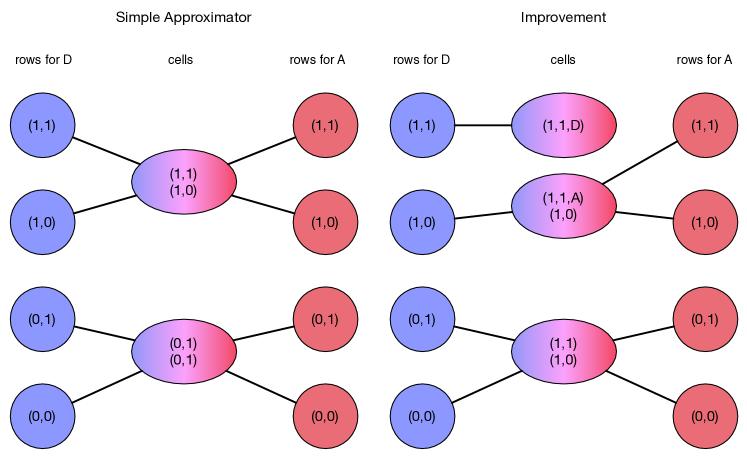
Figure 2: On the left, we have a depiction of the approximator $g_{1}$, which simply groups applicants by the value of ${x}^{\langle 1\rangle}$: the blue and red circles represent the rows associated with $D$ and $A$ respectively, and they are linked to ovals representing the cells that contain them. We can improve both the efficiency and the equity of $g_{1}$ if we use the construction on the right, creating a new cell that pulls out the row $(1,1,D)$ — containing those applicants from group $D$ with ${x}^{\langle 1\rangle}={x}^{\langle 2\rangle}=1$ — and ranking it separately.

4.2 Improving a Simple Approximator

Now, let’s consider a natural example of a simple $f$-approximator, and see how it can be strictly improved. The approximator we consider is $g_{1}$, which creates two cells: $C_{1}$, consisting of all applicants for whom $x^{\langle 1\rangle}=1$, and $C_{2}$, consisting of all applicants for whom $x^{\langle 1\rangle}=0$. Intuitively, this corresponds to projecting the applicants onto just the variable $x^{\langle 1\rangle}$, ignoring the values of $x^{\langle 2\rangle}$ and the group membership $\gamma$.

For $g_{1}$, we have $\mu(C_{1})=p_{1}/2+q_{1}/2=1/2$, and $\mu(C_{2})=1/2$ as well. In this first cell $C_{1}$, the fraction of $D$-applicants is

$$\frac{q_{1}/2}{p_{1}/2+q_{1}/2}=q_{1},$$

and so $W_{g_{1}}(r)=q_{1}$ for all $r\leq 1/2$. The average $f$-value of the applicants in $C_{1}$, working directly from the definition, is $p_{1}p_{2}+q_{1}q_{2}^{\prime}+y_{10}(p_{1}q_{2}+q_{1}p_{2}^{\prime})$, which is close to $p_{1}p_{2}+q_{1}q_{2}^{\prime}$ since $y_{10}$ is very small. This is the value of $V_{g_{1}}(r)$ for all $r\leq 1/2$.

Now, let’s look for a function that strictly improves $g_{1}$. A natural first candidate to consider is $g^{*}$: its efficiency cannot be improved at any admission rate $r$ since it orders all applicants in decreasing order of $f$-value; and subject to this (i.e. as a tie-breaker) it puts $D$-applicants ahead of $A$-applicants. It turns out, though, that there are values of the admission rate $r$ for which $g_{1}$ has better equity than $g^{*}$. In particular, consider $r^{*}=(p_{1}p_{2}+q_{1}q_{2}^{\prime})/2$, when the set $A_{g^{*}}(r^{*})$ admitted according to $g^{*}$ is precisely those applicants with $x^{\langle 1\rangle}=x^{\langle 2\rangle}=1$. For this value of $r^{*}$, we have

$$W_{g^{*}}(r^{*})=\frac{q_{1}q_{2}^{\prime}}{p_{1}p_{2}+q_{1}q_{2}^{\prime}}.$$

But since $r^{*}=(p_{1}p_{2}+q_{1}q_{2}^{\prime})/2<(p_{1}+q_{1})(p_{2}+q_{2}^{\prime})/2<(p_{1}+q_{1})(p_{2}+q_{2})/2=1/2$, we have

$$W_{g_{1}}(r^{*})=q_{1}=\frac{q_{1}q_{2}^{\prime}}{p_{1}q_{2}^{\prime}+q_{1}q_{2}^{\prime}}>\frac{q_{1}q_{2}^{\prime}}{p_{1}p_{2}+q_{1}q_{2}^{\prime}}=W_{g^{*}}(r^{*}),$$

and therefore $g^{*}$ does not strictly improve on $g_{1}$.

Arguably, this calculation implicitly connects to the qualitative intuition that simpler rules may be fairer in general: since the distributions of both $x^{\langle 1\rangle}$ and $x^{\langle 2\rangle}$ confer disadvantage on group $D$, by using only one of them rather than both (thus using $g_{1}$ instead $g^{*}$) we give up some efficiency but we are rewarded by improving equity at a crucial value of the admission rate: specifically, the rate $r^{*}$ corresponding to the fraction of “top applicants” (of $f$-value equal to 1) in the population.

But this intuition is misleading, because in fact there are approximators that improve on $g_{1}$ in both efficiency and equity; it’s just that $g^{*}$ isn’t one of them. An approximator that we can use is $h$, which starts from $g_{1}$ and then splits the cell $C_{1}$ into two cells: $C_{1}^{\prime}$, consisting of applicants from row $(1,1,D)$, and $C_{1}^{\prime\prime}$, consisting of applicants from the three rows $(1,1,A),(1,0,A)$, and $(1,0,D)$. The approximator $h$ thus has the three cells $C_{1}^{\prime},C_{1}^{\prime\prime},C_{2}$, in this order. We can now check that $h$ is at least as good as $g_{1}$ at every admission rate $r$, since it is admitting the applicants of cell $C_{1}$ in a subdivided order — everyone in $C_{1}^{\prime}$ followed by everyone in $C_{1}^{\prime\prime}$ — and the applicants in $C_{1}^{\prime}$ have a higher average $f$-value than the applicants of $C_{1}$, and all of them belong to group $D$. Moreover, this means that when $r=\mu(C_{1}^{\prime})$, we have $V_{h}(r)>V_{g_{1}}(r)$ and $W_{h}(r)>W_{g_{1}}(r)$, and hence $h$ strictly improves $g_{1}$.

Figure 2 shows schematically how we produce $h$ from $g_{1}$. Initially, $g_{1}$ groups all the rows with ${x}^{\langle 1\rangle}=1$ into one cell, and all the rows with ${x}^{\langle 1\rangle}=0$ into another. We then produce $h$ by pulling the row $(1,1,D)$ out of this first cell and turning it into a cell on its own, with both a higher average $f$-value and a positive contribution to the equity.

This example gives a specific instance of the general construction that we will use in proving our first main result (3.12): breaking apart a non-trivial cell so as to admit a subset with both a higher average $f$-value and a higher representation of $D$-applicants. This construction also connects directly to both our earlier discussion of improving simple approximators, and to the line of intuition expressed in the introduction — that simplifying by suppressing variables can prevent the strongest disadvantaged applicants from demonstrating their strength.

$x^{\langle 1\rangle}$	$x^{\langle 2\rangle}$	$\gamma$	$g_{1}$	$\mu$
1	any	any	$p_{1}p_{2}+q_{1}q_{2}^{\prime}+y_{10}(p_{1}q_{2}+q_{1}p_{2}^{\prime})$	1/2
0	any	any	$y_{01}(p_{1}q_{2}^{\prime}+q_{1}p_{2})$	1/2

(a) Approximator $g_{1}$ using only $x^{\langle 1\rangle}$

$x^{\langle 1\rangle}$	$x^{\langle 2\rangle}$	$\gamma$	$\chi(g_{1})$	$\mu$
1	any	$A$	$p_{2}+y_{10}q_{2}$	$p_{1}/2$
1	any	$D$	$q_{2}^{\prime}+y_{10}p_{2}^{\prime}$	$q_{1}/2$
0	any	$A$	$y_{01}p_{2}$	$q_{1}/2$
0	any	$D$	$y_{01}q_{2}^{\prime}$	$p_{1}/2$

(b) Approximator $\chi(g_{1})$ using $x^{\langle 1\rangle}$ and $\gamma$

Figure 3: The $f$-approximator $g_{1}$ has only two cells, based on the value of ${x}^{\langle 1\rangle}$. When we split each of these cells by using the value of the group membership variable $\gamma$ as well, we end up with an $f$-approximator $\chi(g_{1})$ that is strictly better in efficiency and strictly worse in equity. Thus, for a decision-maker interested in maximizing efficiency, the suppression of ${x}^{\langle 2\rangle}$ leads to an incentive to consult the value of group membership, in a way that reduces equity for group $D$.

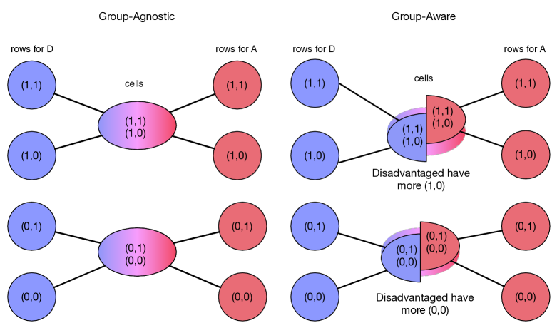
Figure 4: As in Figure 2, the approximator on the left is $g_{1}$, which groups applicants by the value of ${x}^{\langle 1\rangle}$. If we split each of the two cells using group membership, we get the approximator $\chi(g_{1})$ on the right, with four cells in total: two associated with group $A$ and two associated with group $D$. In $\chi(g_{1})$, the cells associated with $A$ have moved slightly upward in value, and the cells associated with $D$ have moved slightly downward in value. As a result, this new approximator $\chi(g_{1})$ is more efficient but less equitable than the original group-agnostic approximator $g_{1}$.

4.3 Adding Group Membership to an Approximator

Because the approximator $g_{1}$ is group-agnostic, we can also use it to provide an example of the effect we see when we move from a group-agnostic approximator $g$ to the version $\chi(g)$ in which we split each of $g$’s cells using group membership.

Specifically, consider the cells of $g_{1}$, denoted $C_{1}$ and $C_{2}$ in the previous subsection. $C_{1}$ groups together the four rows in which ${x}^{\langle 1\rangle}=1$, and $C_{2}$ groups together the four rows in which ${x}^{\langle 1\rangle}=0$. Now, suppose that we split $C_{1}$ into two cells: $C_{1}^{\prime}$ consisting of the two rows in which ${x}^{\langle 1\rangle}=1$ and $\gamma=A$, and $C_{1}^{\prime\prime}$ consisting of the two rows in which ${x}^{\langle 1\rangle}=1$ and $\gamma=D$. Working from the definitions, the average $f$-value of an applicant in $C_{1}^{\prime}$ is $p_{2}+y_{10}q_{2}$, while the average $f$-value of an applicant in $C_{1}^{\prime\prime}$ is $q_{2}^{\prime}+y_{10}p_{2}^{\prime}$. Similarly, if we split $C_{2}$ into cells $C_{2}^{\prime}$ with ${x}^{\langle 1\rangle}=1$ and $\gamma=A$, and $C_{2}^{\prime\prime}$ with ${x}^{\langle 1\rangle}=1$ and $\gamma=D$, then the average $f$-value of an applicant in $C_{2}^{\prime}$ is $y_{01}p_{2}$, while the average $f$-value of an applicant in $C_{2}^{\prime\prime}$ is $y_{01}q_{2}^{\prime}$.

The pair of tables in Figure 3 provides one way of summarizing these calculations: each row represents a cell in which certain variables are fixed and others are set to “any,” meaning that the cell averages over rows with any value allowed for these variables. To go from $g_{1}$ to $\chi(g_{1})$, we convert the first row in the first table into the top two rows in the second table, and we convert the second row in the first table into the bottom two rows in the second table.

We have the sequence of inequalities

$$\theta(C_{1}^{\prime})>\theta(C_{1})>\theta(C_{1}^{\prime\prime})>\theta(C_{2}^{\prime})>\theta(C_{2})>\theta(C_{2}^{\prime\prime}),$$

reflecting the fact that using group membership in conjunction with ${x}^{\langle 1\rangle}$ results in a partition of each cell into a subset with higher average $f$-value and a subset with lower average $f$-value. Since $\chi(g_{1})$ consists of the cells $C_{1}^{\prime},C_{1}^{\prime\prime},C_{2}^{\prime},C_{2}^{\prime\prime}$, it strictly improves $g_{1}$ in efficiency. But since $\chi(g)$ places rows associated with group $A$ ahead of the corresponding rows associated with group $D$, it follows that $g$ strictly improves $\chi(g)$ in equity.

Figure 4 provides another way to depict the transformation from $g_{1}$ to $\chi(g_{1})$: when we split the cells of $g_{1}$ using group membership, the cells associated with group $A$ move slightly upward and the cells associated with group $D$ move slightly downward, producing both the increase in efficiency and the reduction in equity.

Thus, for a decision-maker who wants to maximize efficiency, the $f$-approximator $g_{1}$ creates an incentive to consult the value of $\gamma$ encoding group membership, since doing so leads to a strict improvement in efficiency. The resulting rule $\chi(g_{1})$, however, is explicitly biased against applicants from group $D$, in that it uses group membership information and results in reduced equity for group $D$. This effect wouldn’t have happened had we started from the $f$-approximator $g^{\circ}$ that uses the values of both ${x}^{\langle 1\rangle}$ and ${x}^{\langle 2\rangle}$; in that case, efficiency would not be improved by using group membership information. It is by suppressing information about the value of ${x}^{\langle 2\rangle}$ that $g_{1}$ creates an incentive to incorporate group membership.

5 Proof of First Result: Simple Functions are Improvable

In this section, we prove our first main result in its general form, (3.12). The basic strategy will be an extension of the idea used in the discussion after the statement of (3.9) and in the example from Section 4.2: given a simple (or graded) $f$-approximator $g$, we will show how to break up one or more of its cells, changing the order in which rows are admitted, so that the efficiency and equity don’t decrease, and for some admission rate we are admitting applicants of higher average $f$-value and with a greater fraction of $D$-applicants.

It will turn out that the most challenging case is when we have an $f$-approximator $g$ in which each non-trivial cell consists entirely of rows associated with $A$ or entirely of rows associated with $D$. We will call such an approximator separable (since its non-trivial cells separate the two groups completely); it is easy to verify from the definition of graded approximators in (3.11) that every separable approximator is graded. For this case, we will need to first prove a preliminary combinatorial lemma, which in turn draws on a consequence of the disadvantage condition.

We will work in the general model, where we have an arbitrary set of feature vectors $\{{x}_{1},{x}_{2},\ldots,{x}_{n}\}$, indexed so that $f({x}_{i})<f({x}_{j})$ for $i<j$; this results in a set of $2n$ rows of the form $({x}_{i},\gamma)$ for a group membership variable $\gamma$. We will use $y_{i}$ to denote $f({x}_{i})$, so the set of possible $f$-values is $\{y_{1},\ldots,y_{n}\}$.

5.1 A Consequence of the Disadvantage Condition

It is not hard to show that the disadvantage condition implies that the average $f$-value over the $A$-applicants is higher than the average $f$-value over the $D$-applicants. But we would like to establish something stronger, as follows. For a set of feature vectors $S\subseteq\{{x}_{1},{x}_{2},\ldots,{x}_{n}\}$, let $S_{A}=\{(x_{i},A):{x}_{i}\in S\}$ and $S_{D}=\{(x_{i},D):{x}_{i}\in S\}$. For a set $S$, we let $|S|$ denote the number of elements it has. We will show

(5.1)

For any set of feature vectors $S\subseteq\{{x}_{1},{x}_{2},\ldots,{x}_{n}\}$ with $|S|>1$, we have $\overline{{f}|{S_{A}}}>\overline{{f}|{S_{D}}}$.

Note that for the case when $|S|=1$, we must have $\overline{{f}|{S_{A}}}=\overline{{f}|{S_{D}}}$ because in this case $S$ consists of just a single feature ${x}_{i}$, and by assumption $f({x}_{i},A)=f({x}_{i},D)$ for all $i$.

To prove (5.1), and some of the subsequent results in this section, there is a useful way to think about averages over sets of rows in terms of random variables. We define the random variable $Y_{A}$ to be the $f$-value of an applicant drawn uniformly at random from group $A$, and the random variable $Y_{D}$ to be the $f$-value of an applicant drawn uniformly at random from group $D$. Both of these random variables take values in the set $\{y_{1},\ldots,y_{n}\}$, but they have different distributions over this set; in particular, ${\rm Pr}\left[{Y_{A}=y_{j}}\right]=\mu({x}_{j},A)/\sum_{i=1}^{n}\mu({x}_{i},A)$ and ${\rm Pr}\left[{Y_{D}=y_{j}}\right]=\mu({x}_{j},D)/\sum_{i=1}^{n}\mu({x}_{i},D)$. We will use $\alpha_{j}$ to denote ${\rm Pr}\left[{Y_{A}=y_{j}}\right]$ and $\delta_{j}$ to denote ${\rm Pr}\left[{Y_{D}=y_{j}}\right]$. Note that the disadvantage condition (3.1) implies that the sequence of ratios $\alpha_{i}/\delta_{i}$ is strictly increasing in $i$: if $j>i$, then $\alpha_{j}/\delta_{j}>\alpha_{i}/\delta_{i}$.

In the language of random variables, the disadvantage condition thus asserts that the random variable $Y_{A}$ exhibits likelihood-ratio dominance with respect to the random variable $Y_{D}$ [3, 20, 30, 37]. It is a standard fact from this literature that if one random variable likelihood-ratio dominates another, then it also has a strictly greater expected value [20, 37]. We record this fact here in a general form, since we will need it in some of the subsequent arguments.

(5.2)

(See e.g. [20, 37]) Consider two discrete random variables $P$ and $Q$, each of which takes values in $\{u_{1},u_{2},\ldots,u_{n}\}$, with $u_{1}<u_{2}<\cdots<u_{n}$ and $n>1$. Let $p_{i}={\rm Pr}\left[{P_{i}=u_{i}}\right]$ and $q_{i}={\rm Pr}\left[{Q_{i}=u_{i}}\right]$; so $\sum_{i=1}^{n}p_{i}=\sum_{i=1}^{n}q_{i}=1$, and the expected values are given by $E\left[{P}\right]=\sum_{i=1}^{n}p_{i}u_{i}$ and $E\left[{Q}\right]=\sum_{i=1}^{n}q_{i}u_{i}$. We will assume that $p_{i}>0$ and $q_{i}>0$ for all $i$.

If the sequence of ratios $\{q_{i}/p_{i}\}$ is strictly monotonically increasing then $E\left[{Q}\right]>E\left[{P}\right]$.

For completeness, we give a proof (5.2) in the appendix. Using this fact, we can now give a proof of (5.1).

Proof of (5.1). In the language of random variables, (5.2) is equivalent to showing that for every set $M\subseteq\{y_{1},\ldots,y_{n}\}$ with $|M|>1$, we have $E\left[{Y_{A}}~{}|~{}{Y_{A}\in M}\right]>E\left[{Y_{D}}~{}|~{}{Y_{D}\in M}\right]$.

To prove this, we write $M=\{y_{i_{1}},y_{i_{2}},\ldots,y_{i_{c}}\}$ for $i_{1}<i_{2}<\cdots<i_{c}\subseteq\{1,2,\ldots,n\}$. Let us define $Y_{D}^{\langle M\rangle}$ to be the random variable defined on $M$ by

$${\rm Pr}\left[{Y_{D}^{\langle M\rangle}=y_{i_{j}}}\right]=\frac{\delta_{i_{j}}}{\sum_{\ell=1}^{c}\delta_{i_{\ell}}}.$$

We define $Y_{A}^{\langle M\rangle}$ analogously by

$${\rm Pr}\left[{Y_{A}^{\langle M\rangle}=y_{i_{j}}}\right]=\frac{\alpha_{i_{j}}}{\sum_{\ell=1}^{c}\alpha_{i_{\ell}}}.$$

We observe that $E\left[{Y_{D}^{\langle M\rangle}}\right]=E\left[{Y_{D}}~{}|~{}{Y_{D}\in M}\right]$ and $E\left[{Y_{A}^{\langle M\rangle}}\right]=E\left[{Y_{A}}~{}|~{}{Y_{A}\in M}\right]$. Moreover, we have

$${\rm Pr}\left[{Y_{A}^{\langle M\rangle}=y_{i_{j}}}\right]/{\rm Pr}\left[{Y_{D}^{\langle M\rangle}=y_{i_{j}}}\right]=\frac{\frac{\alpha_{i_{j}}}{\sum_{\ell=1}^{c}\alpha_{i_{\ell}}}}{\frac{\delta_{i_{j}}}{\sum_{\ell=1}^{c}\delta_{i_{\ell}}}}=\frac{\alpha_{i_{j}}\sum_{\ell=1}^{c}\delta_{i_{\ell}}}{\delta_{i_{j}}\sum_{\ell=1}^{c}\alpha_{i_{\ell}}},$$

where the second term in each of the numerator and denominator is independent of $j$; thus, this sequence of ratios is strictly monotonically increasing in $j$ because $\alpha_{i_{j}}/\delta_{i_{j}}$ is. It follows that the likelihood ratio dominance condition as stated in (5.2) holds for the pair of random variables $Y_{A}^{\langle M\rangle}$ and $Y_{D}^{\langle M\rangle}$. Hence by (5.2), we have $E\left[{Y_{A}}~{}|~{}{Y_{A}\in M}\right]=E\left[{Y_{A}^{\langle M\rangle}}\right]>E\left[{Y_{D}^{\langle M\rangle}}\right]=E\left[{Y_{D}}~{}|~{}{Y_{D}\in M}\right].$  

5.2 A Combinatorial Lemma about Separable Approximators

Recall that an $f$-approximator $g$ is called separable if each non-trivial cell consists entirely of rows associated with group $A$ or entirely of rows associated with group $D$. As a key step in the proof of (3.12), we will need the following fact: in any non-trivial, separable $f$-approximator $g$, there exists an $A$-applicant who receives a value that is strictly higher than a $D$-applicant with the same feature vector. Given the disadvantage condition, it is intuitively plausible that this should be true. But given that a number of quite similar-sounding statements are in fact false — essentially, these statements are very close to what arises in Simpson’s Paradox [6] — some amount of care is needed in the proof of this fact. (We explore the connection to Simpson’s Paradox in Section 7.)

(5.3)

Let $g$ be a non-trivial, separable $f$-approximator. Then there exists an $x_{j}$ such that $g$ assigns the row $(x_{j},A)$ a strictly higher value than it assigns the row $(x_{j},D)$. That is, $(x_{j},A)$ and $(x_{j},D)$ belong to cells $C_{a}$ and $C_{b}$ respectively, and $\theta(C_{a})>\theta(C_{b})$, where as before $\theta(C)$ denotes the average $f$-value of the members of a cell $C$.

Proof. Let the cells containing rows of group $D$ be $S_{1},S_{2},\ldots,S_{c}$, and the cells containing rows of group $A$ be $T_{1},T_{2},\ldots,T_{m}$. We define $S(j)$ to be the cell $S_{i}$ for which $(x_{j},D)\in S_{i}$, and we define $T(j)$ to be the cell $T_{\ell}$ for which $(x_{j},A)\in T_{\ell}$. For a set of rows $M$, we also define $y(M)=\{f(\overline{{x}}):\overline{{x}}\in M\}$.

We take care of two initial considerations at the outset. First, $g$ may contain trivial cells of the form $\{(x_{j},A),(x_{j},D)\}$, since separability only requires that each non-trivial cell consist entirely of rows from the same group. We can modify $g$ so that any such trivial cell is replaced instead by the two cells $\{(x_{j},A)\}$ and $\{(x_{j},D)\}$. If we obtain the result for this modified approximator, it will hold for the original approximator $g$ as well. Thus, we will henceforth assume that each cell of $g$ (trivial or non-trivial) consists entirely of rows from the same group.

Second, the result is immediate in the case when all the cells $T_{\ell}$ associated with group $A$ are singletons. Indeed, in this case, since $g$ is non-trivial, there must be a cell $S_{i}$ associated with group $D$ that contains more than one row. We choose such a cell $S_{i}$, let $(x_{j},D)$ be the row in $S_{i}$ of maximum $f$-value, and let $T_{\ell}$ be the (singleton) cell consisting of $\{(x_{j},A)\}$. Then $\theta(S_{i})<f({x}_{j})=\theta(T_{\ell})$, and the result follows. Thus, we will also henceforth assume that at least one cell of $g$ contains multiple rows of $A$.

With these two preliminaries out of the way, we proceed with the main portion of the proof. We again use the random-variable interpretation, in which $Y_{A}$ is the $f$-value of a candidate drawn at random from group $A$, and $Y_{D}$ is the $f$-value of a candidate drawn at random from group $D$. Thus we have $\theta(S_{i})=E\left[{Y_{D}}~{}|~{}{Y_{D}\in y(S_{i})}\right]$ and $\theta(T_{\ell})=E\left[{Y_{A}}~{}|~{}{Y_{A}\in y(T_{\ell})}\right]$.

The statement we are trying to prove requires that we find a choice of $j$ for which the cell containing $(x_{j},D)$ has a strictly lower $\theta$-value than the row containing $(x_{j},A)$ — that is, a $j$ such that $\theta(S(j))<\theta(T(j))$. Using the connection to random variables as just noted, this means we need to find a $j$ for which $E\left[{Y_{D}}~{}|~{}{Y_{D}\in y(S(j))}\right]<E\left[{Y_{A}}~{}|~{}{Y_{A}\in y(T(j))}\right]$.

A useful start is to write

$$E\left[{Y_{D}}\right] = \sum_{i=1}^{c}E\left[{Y_{D}}~{}|~{}{Y_{D}\in y(S_{i})}\right]{\rm Pr}\left[{Y_{D}\in y(S_{i})}\right]$$ (1)

$$= \sum_{i=1}^{c}\left[E\left[{Y_{D}}~{}|~{}{Y_{D}\in y(S_{i})}\right]\sum_{(x_{j},D)\in S_{i}}\delta_{j}\right]$$

$$= \sum_{j=1}^{n}\delta_{j}E\left[{Y_{D}}~{}|~{}{Y_{D}\in y(S(j))}\right]$$

and analogously, for $Y_{A}$, we have

$$E\left[{Y_{A}}\right] = \sum_{\ell=1}^{m}E\left[{Y_{A}}~{}|~{}{Y_{A}\in y(T_{\ell})}\right]{\rm Pr}\left[{Y_{A}\in y(T_{\ell})}\right]$$ (2)

$$= \sum_{\ell=1}^{m}\left[E\left[{Y_{A}}~{}|~{}{Y_{A}\in y(T_{\ell})}\right]\sum_{(x_{j},A)\in T_{\ell}}\alpha_{j}\right]$$

$$= \sum_{j=1}^{n}\alpha_{j}E\left[{Y_{A}}~{}|~{}{Y_{A}\in y(T(j))}\right]$$

Given that $E\left[{Y_{D}}\right]<E\left[{Y_{A}}\right]$, this immediately tells us that there is a $j$ for which

$$\delta_{j}E\left[{Y_{D}}~{}|~{}{Y_{D}\in y(S(j))}\right]<\alpha_{j}E\left[{Y_{A}}~{}|~{}{Y_{A}\in y(T(j))}\right].$$

But this doesn’t actually get us very far, because the terms we care about ($E\left[{Y_{D}}~{}|~{}{Y_{D}\in y(S(j))}\right]$ and $E\left[{Y_{A}}~{}|~{}{Y_{A}\in y(T(j))}\right]$) are being multipled by different coefficients on the two sides of the inequality ($\delta_{j}$ and $\alpha_{j}$ respectively). This is a non-trivial point, since in fact the statement we are trying to prove would not in fact hold if the only thing we knew about the random variables $Y_{D}$ and $Y_{A}$ were the inequality $E\left[{Y_{D}}\right]<E\left[{Y_{A}}\right]$. (We explore this point further in Section 7.) Thus, we must use additional structure in the values of $\delta_{j}$ and $\alpha_{j}$; in particular, we will apply the disadvantage condition (3.1) and its consequence (5.1).

The idea will be to interpose a new quantity that we can compare with both $E\left[{Y_{D}}~{}|~{}{Y_{D}\in y(S(j))}\right]$ and $E\left[{Y_{A}}~{}|~{}{Y_{A}\in y(T(j))}\right]$ for any given index $j$, and which in this way will allow us to compare these two quantities to each other by transitivity. To do this, we first observe that Equation (1) applies to any partition of the rows of group $D$. We therefore invoke this equation for a second partition of the rows of group $D$ — in particular, we will partition the rows of $D$ in a way that “lines up” with the partition $T_{1},T_{2},\ldots,T_{m}$ used for the rows of group $A$. With this in mind, we define the following partition of the rows associated with $D$: we write $T_{\ell}^{\prime}=\{(x_{j},D):(x_{j},A)\in T_{\ell}\}$. As above, we define $T^{\prime}(j)$ to be the set $T_{\ell}^{\prime}$ for which $(x_{j},D)\in T_{\ell}^{\prime}$. Following the same argument as in Equation (1), we have

$$E\left[{Y_{D}}\right]=\sum_{j=1}^{n}\delta_{j}E\left[{Y_{D}}~{}|~{}{Y_{D}\in y(T^{\prime}(j))}\right].$$

Subtracting this from Equation (1) for $E\left[{Y_{D}}\right]$, we get

$$\sum_{j=1}^{n}\delta_{j}\left(E\left[{Y_{D}}~{}|~{}{Y_{D}\in y(S(j))}\right]-E\left[{Y_{D}}~{}|~{}{Y_{D}\in y(T^{\prime}(j))}\right]\right)=0.$$ (3)

It will turn out to matter in the remainder of the proof whether or not the index $j$ we are working with has the property that $T^{\prime}(j)$ is a singleton set (i.e. with $|T^{\prime}(j)|=1$). Therefore, viewing the left-hand side of Equation (3) as a sum over $n$ terms, we group these terms into two sets: let $K$ be the sum over all terms $j$ for which $T^{\prime}(j)$ is a singleton, and let $L$ be the sum over all terms $j$ for which $|T^{\prime}(j)|>1$. Recall that since we addressed the case in which all sets $T_{\ell}$ (and hence all sets $T_{\ell}^{\prime}$) are singletons, we can assume that at least one of the sets $T_{\ell}^{\prime}$ has size greater than 1. Thus, the quantity $L$ is a sum over a non-empty set of terms. In the event that there are no singleton sets $T_{\ell}^{\prime}$ (in which case there are no terms contributing to the value of $K$), we declare $K=0$. Now, the left-hand side of Equation (3) by definition is $K+L$, and so $K+L=0$. Thus, we cannot have both $K\geq 0$ and $L>0$, and so one of $K<0$ or $L\leq 0$ must hold. If $K<0$, then there must be a $j^{*}$ for which $T(j^{*})$ is a singleton and $E\left[{Y_{D}}~{}|~{}{Y_{D}\in y(S(j^{*}))}\right]<E\left[{Y_{D}}~{}|~{}{Y_{D}\in y(T^{\prime}(j^{*}))}\right]$. Alternately, if $L\leq 0$, then there is a $j^{*}$ for which $T(j^{*})$ is not a singleton, and $E\left[{Y_{D}}~{}|~{}{Y_{D}\in y(S(j^{*}))}\right]\leq E\left[{Y_{D}}~{}|~{}{Y_{D}\in y(T^{\prime}(j^{*}))}\right]$.

In summary, we have thus found an index $j^{*}$ for which

$$E\left[{Y_{D}}~{}|~{}{Y_{D}\in y(S(j^{*}))}\right]\leq E\left[{Y_{D}}~{}|~{}{Y_{D}\in y(T^{\prime}(j^{*}))}\right].$$ (4)

and with the additional property that the inequality is strict in the case that $T^{\prime}(j^{*})$ is a singleton.

We now claim that for this $j^{*}$, we have

$$E\left[{Y_{D}}~{}|~{}{Y_{D}\in y(S(j^{*}))}\right]<E\left[{Y_{A}}~{}|~{}{Y_{A}\in y(T(j^{*}))}\right].$$ (5)

As discussed at the outset of the proof, this will establish the result, since it says that $(x_{j^{*}},D)$ and $(x_{j^{*}},A)$ belong to cells $S(j^{*})$ and $T(j^{*})$ respectively, and

$$\theta(S(j^{*}))=E\left[{Y_{D}}~{}|~{}{Y_{D}\in y(S(j^{*}))}\right]<E\left[{Y_{A}}~{}|~{}{Y_{A}\in y(T(j^{*}))}\right]=\theta(T(j^{*})).$$

We establish this claim by considering two cases.

Case 1: $|T^{\prime}(j^{*})|>1$. In this case we can apply (5.1) to conclude that $E\left[{Y_{D}}~{}|~{}{Y_{D}\in y(T^{\prime}(j^{*}))}\right]<E\left[{Y_{A}}~{}|~{}{Y_{A}\in y(T(j^{*}))}\right]$. Combining this with Inequality (4), we obtain Inequality (5) by transitivity.

Case 2: $|T^{\prime}(j^{*})|=1$. Above, we noted that our choice of $j^{*}$ ensures that Inequality (4) is strict when $T^{\prime}(j^{*})$ is a singleton, and so we have

$$E\left[{Y_{D}}~{}|~{}{Y_{D}\in y(S(j^{*}))}\right]<E\left[{Y_{D}}~{}|~{}{Y_{D}\in y(T^{\prime}(j^{*}))}\right]$$

in this case. Since $T^{\prime}(j^{*})$ is a singleton, consisting only of the row $({x}_{j^{*}},D)$, we also have

$$E\left[{Y_{D}}~{}|~{}{Y_{D}\in y(T^{\prime}(j^{*}))}\right]=E\left[{Y_{A}}~{}|~{}{Y_{A}\in y(T(j^{*}))}\right],$$

since both the left- and right-hand sides are equal to $f({x}_{j^{*}})$. Combining this with the previous inequality, we obtain Inequality (5) in this case as well.  

5.3 Proof

We now have all the ingredients needed for proving the first main result.

Proof of (3.12). Let $g$ be a graded $f$-approximator with cells $C_{1},\ldots,C_{d}$; thus $g$ is discrete $f$-approximator $g$ with (by non-triviality) at least one cell containing rows $\overline{{x}},\overline{{x}}^{\prime}$ such that $f(\overline{{x}})\neq f(\overline{{x}}^{\prime})$, and such that for every cell $C_{i}$, we have $C_{i}^{\langle A\rangle}\subseteq C_{i}^{\langle D\rangle}$ or $C_{i}^{\langle D\rangle}\subseteq C_{i}^{\langle A\rangle}$. We will create a new $f$-approximator $g^{\prime}$ that strictly improves on $g$.

For an index $\ell$, recall that $r_{\ell}^{\langle g\rangle}$ is the measure of the first $\ell$ entries in the list of cells of $g$. It is also useful to introduce a further piece of notation for the proof: we write $V^{*}_{g}(r)=\int_{0}^{r}v_{g}(t)~{}dt$ for the unnormalized version of $V_{g}(r)$ in which we do not divide by $r$, and we write $W^{*}_{g}(r)=\int_{0}^{r}w_{g}(t)~{}dt$ analogously. In order to show that an approximator $g^{\prime}$ improves on $g$, we can compare the pairs of functions $V^{*}_{g},V^{*}_{g^{\prime}}$ and $W^{*}_{g},W^{*}_{g^{\prime}}$ rather than $V_{g},V_{g^{\prime}}$ and $W_{g},W_{g^{\prime}}$ in the underlying definition. That is, it would be equivalent to our earlier definitions of improvement to say that $g^{\prime}$ weakly improves on $g$ if $V^{*}_{g^{\prime}}(r)\geq V^{*}_{g}(r)$ and $W^{*}_{g^{\prime}}(r)\geq W^{*}_{g}(r)$ for all $r\in(0,1]$; and $g^{\prime}$ strictly improves on $g$ if $g^{\prime}$ weakly improves on $g$, and there exists $r^{*}\in(0,1]$ for which $V^{*}_{g^{\prime}}(r^{*})>V^{*}_{g}(r^{*})$ and $W^{*}_{g^{\prime}}(r^{*})>W^{*}_{g}(r^{*})$.

Inside the proof, it will also be useful to work with objects that are slightly more general than $f$-approximators (although the statement of the result itself applies only to $f$-approximators as we have defined them thus far). In particular, we will say that $h$ is an $f$-pseudo-approximator if it can be obtained from an $f$-approximator $g$ by possibly rearranging the order of the cells so that they are no longer in decreasing order of $\theta$-values. We can still consider admissions rules based on pseudo-approximators $h$ just as we have for approximators $g$: applicants are admitted according to the sequence of cells in $h$, even though they no longer have decreasing $\theta$-values. We can also still define $v_{h},V^{*}_{h},w_{h}$, and $W^{*}_{h}$ for pseudo-approximators just as we do for approximators, and use them in the definitions of weak and strict improvement.

We organize the proof into a set of cases. Each case follows the structure outlined in the discussion after the statement of (3.9): we find a row — or a small portion of a row — that we can break loose from its current cell and convert into a cell on its own; we then place it at the position determined by its value in the overall ordering of cells so as to strictly improve the effiency and the equity of the approximator. Depending on the structure of the initial approximator $g$, we will go about selecting the row to use for this improvement in different ways. This distinction is what determines the decomposition of the proof into cases, but the cases otherwise follow a parallel structure.

Case 1: There is a non-trivial cell $C_{i}$ such that both $C_{i}^{\langle A\rangle}$ and $C_{i}^{\langle D\rangle}$ are non-empty, and $C_{i}^{\langle A\rangle}\subseteq C_{i}^{\langle D\rangle}$. Of all the rows $\overline{{x}}\in C_{i}$, we choose one of maximum $f(\overline{{x}})$. For such an $\overline{{x}}$, we have $f(\overline{{x}})>\theta(C_{i})$, since $\theta(C_{i})$ is an average of $f$-values from multiple rows. Also, at least one row of maximum $f$-value must be associated with group $D$, since for all $({x}_{j},A)\in C_{i}$ we also have $({x}_{j},D)\in C_{i}$; we choose $\overline{{x}}$ so that it is associated with group $D$.

From this row $\overline{{x}}=(x_{j},D)$, we create a new (non-discrete) $f$-approximator $g^{\prime}$ as follows. For a small value ${\varepsilon}>0$, we create a new cell $C^{\prime}$ that contains an ${\varepsilon}$ measure of row $\overline{{x}}$ and nothing else. We correspondingly subtract an ${\varepsilon}$ measure of row $\overline{{x}}$ from cell $C_{i}$, creating a new cell $C_{i}^{\prime}$. This defines the new approximator $g^{\prime}$.

These new cells have the property that $\theta(C^{\prime})>\theta(C_{i})>\theta(C_{i}^{\prime})$, since $\theta(C_{i})$ is a weighted average of $f$-values among which $\theta(C^{\prime})=f(\overline{{x}})$ is the largest. The new cell $C^{\prime}$ thus moves ahead of $C_{i}$ in the sorted order, to position $s<i$. By the genericity condition (3.2), we know that $\theta(C_{i})$ is distinct from the $\theta$-value of all other cells, and so by choosing ${\varepsilon}$ sufficiently small, $C_{i}^{\prime}$ will retain its position in the sorted order of the other cells.

The new approximator has cells

$$C_{1},\ldots,C_{s-1},C^{\prime},C_{s},\ldots,C_{i-1},C_{i}^{\prime},C_{i+1},\ldots,C_{d}$$

in sorted order. Observe that $r_{s-1}^{\langle g\rangle}$ is the measure of the cells in the list preceding $C^{\prime}$, and $r_{i}^{\langle g\rangle}$ is the measure of the cells through $C_{i}^{\prime}$. (For this latter point, note that there are $i+1$ entries in the list of cells of $g^{\prime}$ through $C_{i}^{\prime}$, but since two of these cells are a partition of $C_{i}$, the total measure of these $i+1$ cells is $r_{i}^{\langle g\rangle}$.)

For comparing the functions $V^{*}_{g}$ and $V^{*}_{g^{\prime}}$, it is useful to interpose the following pseudo-approximator $h$. The pseudo-approximator $h$ is obtained by writing the cells of $g^{\prime}$ in the order

$$C_{1},\ldots,C_{s-1},C_{s},\ldots,C_{i-1},C^{\prime},C_{i}^{\prime},C_{i+1},\ldots,C_{d}$$

rather than in their sorted order. As noted above, we can still define $v_{h},V^{*}_{h},w_{h}$, and $W^{*}_{h}$ as before, and use them in the definition of weak and strict improvement.

We observe first that $V^{*}_{g}$ and $V^{*}_{h}$ agree outside the interval $[r_{i-i}^{\langle g\rangle},r_{i}^{\langle g\rangle}]$, and inside this interval we have $V^{*}_{h}(r)>V^{*}_{g}(r)$, since $\theta(C^{\prime})>\theta(C_{i}^{\prime})$. Similarly, $W^{*}_{g}$ and $w_{h}$ agree outside the interval $[r_{i-i}^{\langle g\rangle},r_{i}^{\langle g\rangle}]$, and inside this interval we have $W^{*}_{h}(r)>W^{*}_{g}(r)$, since $\sigma(C^{\prime})=1$ and $\sigma(C_{i}^{\prime})<1$. Thus, $h\succ g$.

Now, we obtain $g^{\prime}$ from $h$ by moving the cell $C^{\prime}$ forward to position $s$ in the sorted order. The functions $V^{*}_{g^{\prime}}$ and $V^{*}_{h}$ are thus the same for $r\leq r_{s-1}^{\langle g\rangle}$ and $r\geq r_{i}^{\langle g\rangle}$. In the interval $(r_{s-1}^{\langle g\rangle},r_{i}^{\langle g\rangle})$, they differ in that we have moved the cell $C^{\prime}$ forward to the beginning of this interval. For all $r\in(r_{s-1}^{\langle g\rangle},r_{i}^{\langle g\rangle})$, we have $\theta(C^{\prime})\geq\theta(C_{j(r)})$ because $C^{\prime}$ comes earlier in the sorted order, and $1=\sigma(C^{\prime})\geq\sigma(C_{j(r)})$. Thus, $V^{*}_{g^{\prime}}(r)\geq V^{*}_{h}(r)$ and $W^{*}_{g^{\prime}}(r)\geq W^{*}_{h}(r)$ for all $r\in(r_{s-1}^{\langle g\rangle},r_{i}^{\langle g\rangle})$ and so we have $g^{\prime}\succeq h$.

By our result (3.6) on transitivity, it follows that $g^{\prime}\succ g$.

Case 2: There is a cell $C_{i}$ such that both $C_{i}^{\langle A\rangle}$ and $C_{i}^{\langle D\rangle}$ are non-empty, and $C_{i}^{\langle D\rangle}\subseteq C_{i}^{\langle A\rangle}$. We proceed by close analogy with Case 1, except that instead of removing a small measure of a row $(x_{j},D)$ of high $f$-value from $C_{i}$, we remove a small measure of a row $(x_{j},A)$ of low $f$-value. Specifically, of all the rows $\overline{{x}}\in C_{i}$, we choose one of minimum $f(\overline{{x}})$. For this $\overline{{x}}$, we have $f(\overline{{x}})<\theta(C_{i})$, and we can choose $\overline{{x}}$ to have the form $(x_{j},A)$, since for all $({x}_{j},D)\in C_{i}$ we also have $({x}_{j},A)\in C_{i}$.

For a small value ${\varepsilon}>0$, we create a new cell $C^{\prime}$ that contains an ${\varepsilon}$ measure of row $\overline{{x}}$ and nothing else. We correspondingly subtract an ${\varepsilon}$ measure of row $\overline{{x}}$ from cell $C_{i}$, creating a new cell $C_{i}^{\prime}$. This defines the new approximator $g^{\prime}$. The new cell $C^{\prime}$ moves after $C_{i}$ in the sorted order, to position $t>i$, and by choosing ${\varepsilon}$ sufficiently small, $C_{i}^{\prime}$ retains its position; so the new approximator $g^{\prime}$ has cells

$$C_{1},\ldots,C_{i-1},C_{i}^{\prime},C_{i+1},\ldots,C_{t-1},C^{\prime},C_{t},\ldots,C_{d}.$$

As in Case 1, we interpose a pseudo-approximator $h$ with the same cells as $g^{\prime}$, but in an order that is not necessarily sorted:

$$C_{1},\ldots,C_{i-1},C_{i}^{\prime},C^{\prime},C_{i+1},\ldots,C_{t-1},C_{t},\ldots,C_{d}.$$

Now, $V^{*}_{g}$ and $V^{*}_{h}$ agree outside the interval $[r_{i-i}^{\langle g\rangle},r_{i}^{\langle g\rangle}]$, and inside this interval we have $V^{*}_{h}(r)>V^{*}_{g}(r)$, since $\theta(C_{i}^{\prime})>\theta(C^{\prime})$. Similarly, $W^{*}_{g}$ and $W^{*}_{h}$ agree outside the interval $[r_{i-i}^{\langle g\rangle},r_{i}^{\langle g\rangle}]$, and inside this interval we have $W^{*}_{h}(r)>W^{*}_{g}(r)$, since $\sigma(C_{i}^{\prime})>0$ and $\sigma(C^{\prime})=0$. Thus, $h\succ g$.

Now, we obtain $g^{\prime}$ from $h$ by moving the cell $C^{\prime}$ back to position $t$ in the sorted order. The functions $V^{*}_{g^{\prime}}$ and $V^{*}_{h}$ are thus the same for $r\leq r_{i-1}^{\langle g\rangle}$ and $r\geq r_{t-1}^{\langle g\rangle}$. In the interval $(r_{i-1}^{\langle g\rangle},r_{t-1}^{\langle g\rangle})$, they differ in that we have moved the cell $C^{\prime}$ back to the end of this interval. For all $r\in(r_{i-1}^{\langle g\rangle},r_{t-1}^{\langle g\rangle})$, we have $\theta(C^{\prime})\leq\theta(C_{j(r)})$ because $C^{\prime}$ comes later in the sorted order, and $0=\sigma(C^{\prime})<\sigma(C_{i}^{\prime})$. Thus, $V^{*}_{g^{\prime}}(r)\geq V^{*}_{h}(r)$ and $W^{*}_{g^{\prime}}(r)\geq W^{*}_{h}(r)$ for all $r\in(r_{i-1}^{\langle g\rangle},r_{t-1}^{\langle g\rangle})$ and so we have $g^{\prime}\succeq h$. By transitivity, it follows that $g^{\prime}\succ g$.

If neither of Cases 1 or 2 holds, then every non-trivial cell of $g$ consists entirely of rows associated with $A$ or entirely of rows associated with $D$. Thus our final case is the following.

Case 3: $g$ is separable. In this case, (5.3) implies that there is an $x_{j}$ such that $(x_{j},A)$ and $(x_{j},D)$ belong to cells $C_{a}$ and $C_{b}$ respectively, and $\theta(C_{a})>\theta(C_{b})$. This case follows a similar high-level strategy to Cases 1 and 2, but using the existence of $x_{j}$ and the cells $C_{a}$ and $C_{b}$ to create a new cell. The construction of this new cell involves moving a small amount of measure out of $C_{a}$ or $C_{b}$, and in some cases out of both cells. For this case, we consider a set of sub-cases, depending on the relative ordering of $f(x_{j})$ with respect to $\theta(C_{a})$ and $\theta(C_{b})$.

Case 3a: $f(x_{j})\geq\theta(C_{a})>\theta(C_{b})$. We define an $f$-approximator $g^{\prime}$ by creating a new cell $C^{\prime}$ that, for a small ${\varepsilon}>0$, contains an ${\varepsilon}$ measure of row $(x_{j},D)$ and nothing else. We correspondingly subtract an ${\varepsilon}$ measure of row $(x_{j},D)$ from cell $C_{b}$, creating a new cell $C_{b}^{\prime}$. We put $C^{\prime}$ in its appropriate place in the sorted order of cells, and ahead of $C_{a}$ in the case that $f(x_{j})=\theta(C_{a})$; so $C^{\prime}$ goes into some position $s\leq a$. The cells of $g^{\prime}$ in order are thus

$$C_{1},\ldots,C_{s-1},C^{\prime},C_{s},\ldots,C_{a},\ldots,C_{b-1},C_{b}^{\prime},C_{b+1},\ldots,C_{d},$$

where possibly $C_{s}=C_{a}$. We also consider the pseudo-approximator $h$ with these same cells in the order

$$C_{1},\ldots,C_{s-1},C_{s},\ldots,C_{a},\ldots,C_{b-1},C^{\prime},C_{b}^{\prime},C_{b+1},\ldots,C_{d}.$$

The functions $V^{*}_{g}$ and $V^{*}_{h}$ agree outside the interval $(r_{b-1}^{\langle g\rangle},r_{b}^{\langle g\rangle})$, and for $r$ in this interval we have $V^{*}_{h}(r)>V^{*}_{g}(r)$. When we then move $C^{\prime}$ forward to its correct position in sorted order, producing $g^{\prime}$, we see that the functions $V^{*}_{g}$ and $V^{*}_{g^{\prime}}$ agree outside the interval $(r_{s-1}^{\langle g\rangle},r_{b}^{\langle g\rangle})$; and for $r$ in this interval, we have $V^{*}_{g^{\prime}}(r)>V^{*}_{g}(r)$.

Similarly, the functions $W^{*}_{g}$ and $W^{*}_{g^{\prime}}$ agree for $r\leq r_{s-1}^{\langle g\rangle}$ and $r\geq r_{b}^{\langle g\rangle}$. For $r_{s-1}^{\langle g\rangle}<r<r_{b}^{\langle g\rangle}$, the functions $W^{*}_{g}$ and $W^{*}_{g^{\prime}}$ differ in the fact that cell $C^{\prime}$ with $\sigma(C^{\prime})=1$ was moved ahead of $C_{s}$, so for all such $r$ we have $W^{*}_{g^{\prime}}(r)\geq W^{*}_{g}(r)$. Now, let $C_{\ell}$ be the next cell after $C^{\prime}$ for which $\sigma(C_{\ell})<1$; we have $\ell\leq a$, since $\sigma(C_{a})=0$. For $r_{\ell}^{\langle g^{\prime}\rangle}<r<r_{\ell+1}^{\langle g^{\prime}\rangle}$, the marginal applicant is being drawn from $C_{\ell}$, and hence $W^{*}_{g^{\prime}}(r)>W^{*}_{g}(r)$ for such $r$. Since this $r$ is also in the range noted above where $V^{*}_{g^{\prime}}(r)>V^{*}_{g}(r)$, we have $g^{\prime}\succ g$.

Case 3b: $\theta(C_{a})>\theta(C_{b})\geq f(x_{j})$. We define an $f$-approximator $g^{\prime}$ by creating a new cell $C^{\prime}$ that, for a small ${\varepsilon}>0$, contains an ${\varepsilon}$ measure of row $(x_{j},A)$ and nothing else. We correspondingly subtract an ${\varepsilon}$ measure of row $(x_{j},A)$ from cell $C_{a}$, creating a new cell $C_{a}^{\prime}$. We put $C^{\prime}$ in its appropriate place in the sorted order of cells, and after $C_{b}$ in the case that $f(x_{j})=\theta(C_{b})$; so $C^{\prime}$ goes into some position $t>b$. The cells of $g^{\prime}$ in order are thus

$$C_{1},\ldots,C_{a-1},C_{a}^{\prime},C_{a+1},\ldots,C_{b},\ldots,C_{t-1},C^{\prime},C_{t},\ldots,C_{d}.$$

We also consider the pseudo-approximator $h$ with these same cells in the order

$$C_{1},\ldots,C_{a-1},C_{a}^{\prime},C^{\prime},C_{a+1},\ldots,C_{b},\ldots,C_{t-1},C_{t},\ldots,C_{d}.$$

The functions $V^{*}_{g}$ and $V^{*}_{h}$ agree outside the interval $(r_{a-1}^{\langle g\rangle},r_{a}^{\langle g\rangle})$, and for $r$ in this interval we have $V^{*}_{h}(r)>V^{*}_{g}(r)$. When we then move $C^{\prime}$ back to its correct position in sorted order, producing $g^{\prime}$, we see that the functions $V^{*}_{g}$ and $V^{*}_{g^{\prime}}$ agree outside the interval $(r_{a-1}^{\langle g\rangle},r_{t-1}^{\langle g\rangle})$; and for $r$ in this interval, we have $V^{*}_{g^{\prime}}(r)>V^{*}_{g}(r)$.

The functions $W^{*}_{g}$ and $W^{*}_{g^{\prime}}$ agree for $r\leq r_{a-1}^{\langle g\rangle}$ and $r\geq r_{t-1}^{\langle g\rangle}$. For $r_{a-1}^{\langle g\rangle}<r<r_{t-1}^{\langle g\rangle}$, the functions $W^{*}_{g}$ and $W^{*}_{g^{\prime}}$ differ in the fact that cell $C^{\prime}$ with $\sigma(C^{\prime})=0$ was moved after $C_{t-1}$, so for all such $r$ we have $W^{*}_{g^{\prime}}(r)\geq W^{*}_{g}(r)$. Now, let $C_{\ell}$ be the next cell after $C_{a}^{\prime}$ for which $\sigma(C_{\ell})>0$; we have $\ell\leq b$, since $\sigma(C_{b})=1$. For $r_{\ell}^{\langle g^{\prime}\rangle}<r<r_{\ell+1}^{\langle g^{\prime}\rangle}$, the marginal applicant is being drawn from $C_{\ell}$, and hence $W^{*}_{g^{\prime}}(r)>W^{*}_{g}(r)$ for such $r$. Since this $r$ is also in the range noted above where $V^{*}_{g^{\prime}}(r)>V^{*}_{g}(r)$, we have $g^{\prime}\succ g$.

Case 3c: $\theta(C_{a})>f(x_{j})>\theta(C_{b}).$ In this case, we define an $f$-approximator $g^{\prime}$ by creating a new cell $C^{\prime}$ that, for a small ${\varepsilon}>0$, contains an ${\varepsilon}$ measure of row $(x_{j},A)$ and an ${\varepsilon}$ measure of row $(x_{j},D)$. We correspondingly subtract an ${\varepsilon}$ measure of row $(x_{j},A)$ from cell $C_{a}$, creating a new cell $C_{a}^{\prime}$, and we subtract an ${\varepsilon}$ measure of row $(x_{j},D)$ from cell $C_{b}$, creating a new cell $C_{b}^{\prime}$. We put $C^{\prime}$ in its appropriate place in the sorted order of cells, which is in some position $i$ with $a<i\leq b$. The cells of $g^{\prime}$ in order are thus

$$C_{1},\ldots,C_{a-1},C_{a}^{\prime},\ldots,C^{\prime},\ldots,C_{b}^{\prime},C_{b+1},\ldots,C_{d}.$$

We consider two pseudo-approximators $h$ and $h^{\prime}$. For these, we define $C_{a}^{+}$ to be a cell consisting only of an ${\varepsilon}$ measure of row $(x_{j},A)$, and we define $C_{b}^{+}$ to be a cell consisting only of an ${\varepsilon}$ measure of row $(x_{j},D)$. Note that $C^{\prime}$ is obtained by merging $C_{a}^{+}$ and $C_{b}^{+}$ together. We define $h$ to have the sequence of cells

$$C_{1},\ldots,C_{a-1},C_{a}^{\prime},C_{a}^{+},\ldots,C_{b}^{+},C_{b}^{\prime},C_{b+1},\ldots,C_{d}.$$

We define $h^{\prime}$ to be obtained from $h$ by shifting $C_{a}^{+}$ later if necessary and $C_{b}^{+}$ forward if necessary so they are consecutive in position $i$.

Now, the functions $V^{*}_{g}$ and $V^{*}_{h}$ agree outside the intervals $(r_{a-1}^{\langle g\rangle},r_{a}^{\langle g\rangle})$ and $(r_{b-1}^{\langle g\rangle},r_{b}^{\langle g\rangle})$; inside these intervals we have $V^{*}_{h}(r)>V^{*}_{g}(r)$. When we move $C_{a}^{+}$ and $C_{b}^{+}$ to be adjacent in position $i$, we obtain $h^{\prime}$ with $V^{*}_{h^{\prime}}(r)>V^{*}_{g}(r)$ for $r\in(r_{a-1}^{\langle g\rangle},r_{b}^{\langle g\rangle})$ (and the same function outside this interval). Finally, $V^{*}_{h^{\prime}}$ and $V^{*}_{g^{\prime}}$ are the same function everywhere.

The functions $W^{*}_{g}$ and $W^{*}_{h^{\prime}}$ agree for $r\leq r_{a-1}^{\langle g\rangle}$ and $r\geq r_{b}^{\langle g\rangle}$. For $r_{a-1}^{\langle g\rangle}<r<r_{b}^{\langle g\rangle}$, the functions $W^{*}_{g}$ and $W^{*}_{h^{\prime}}$ differ in the fact that cell $C_{a}^{+}$ with $\sigma(C_{a}^{+})=0$ was moved after $C_{i-1}$, and cell $C_{b}^{+}$ with $\sigma(C_{b}^{+})=1$ was moved forward to be just behind it; so for all $r\in(r_{a-1}^{\langle g\rangle},r_{b}^{\langle g\rangle})$ we have $W^{*}_{h^{\prime}}(r)\geq W^{*}_{g}(r)$. Since $g^{\prime}$ is obtained from $h^{\prime}$ by simply combining the adjacent cells $C_{a}^{+}$ and $C_{b}^{+}$ into the single cell $C^{\prime}$, we have $W^{*}_{g^{\prime}}(r)\geq W^{*}_{h^{\prime}}(r)$ for all $r$. Now, let $C_{\ell}$ be the next cell of $g^{\prime}$ after $C_{a}^{\prime}$ for which $\sigma(C_{\ell})>0$; $C_{\ell}$ must be before or equal to $C^{\prime}$, since $\sigma(C^{\prime})=1/2$. For $r_{\ell-1}^{\langle g^{\prime}\rangle}<r<r_{\ell}^{\langle g^{\prime}\rangle}$, the marginal applicant is from $C_{\ell}$, so $W^{*}_{g^{\prime}}(r)>W^{*}_{g}(r)$ for such $r$. Since this $r$ is in the range noted above where $V^{*}_{g^{\prime}}(r)>V^{*}_{g}(r)$, we have $g^{\prime}\succ g$.  

5.4 The Role of Non-Discrete Approximators

The proof of (3.12) showed how an arbitrary graded $f$-approximator $g$ could be improved by another $f$-approximator $g^{\prime}$. The construction in the proof produced $f$-approximators that were not necessarily discrete, and it is natural to ask whether the use of non-discrete approximators was esssential for the result; is it possible that for every graded $f$-approximator, there is a discrete $f$-approximator that strictly improves it?

In fact, there exist graded $f$-approximators $g$ such that every approximator strictly improving $g$ is non-discrete; this establishes that non-discrete approximators are indeed necessary for the result. In this section, we give an example of such a graded approximator.

We use the example from Figure 1 in Section 4, with the parameters $y_{10}$ and $y_{01}$ close enough to 0 so that the following holds: if $S$ is the set of three rows $\{(1,1,D),(0,1,D),(0,0,D)\}$, then $\overline{{f}|{S}}>f(1,0,D)$. For the function $f$ given in Figure 1, consider the following $f$-approximator $g$: it consists of cells $C_{1},C_{2},\ldots,C_{6}$, where $C_{1}$ is the row $(1,1,A)$, $C_{2}=S$, and $C_{3},C_{4},C_{5},C_{6}$ are each singleton sets consisting of the rows $(1,0,D)$, $(1,0,A)$, $(0,1,A)$, and $(0,0,A)$ respectively.

If we follow the construction used in the proof of (3.12), we arrive at the following non-discrete $f$-approximator $g^{\prime}$ that strictly improves $g$. Let $C_{0}({\varepsilon})$ be the cell consisting of an ${\varepsilon}$ measure of the row $(1,1,D)$, and let $C_{2}^{\prime}({\varepsilon})$ be the cell we obtain by starting with $C_{2}$ and removing an ${\varepsilon}$ measure of the row $(1,1,D)$. We also define the cell $C_{2}^{\prime\prime}({\varepsilon})$ to consist of $C_{2}^{\prime}({\varepsilon})$ together with $C_{3}$. As we increase ${\varepsilon}$, the value of $\theta(C_{2}^{\prime}({\varepsilon}))$ decreases monotonically; and by the time ${\varepsilon}$ reaches $\mu(1,1,D)$, we have $\theta(C_{2}^{\prime}({\varepsilon}))<\theta(C_{3})$, since for this value of ${\varepsilon}$, the cell $C_{2}^{\prime}({\varepsilon})$ consists of just the rows $(0,1,D)$ and $(0,0,D)$. We can therefore find an ${\varepsilon}^{*}>0$ such that $\theta(C_{2}^{\prime}({\varepsilon}))=\theta(C_{3})$, and we define the $f$-approximator $g^{\prime}$ to consist of the cells

$$C_{0}({\varepsilon}^{*}),C_{1},C_{2}^{\prime\prime}({\varepsilon}^{*}),C_{4},C_{5},C_{6}.$$

$g^{\prime}$ is a non-discrete $f$-approximator that strictly improves $g$.

However, it turns out that the only $f$-approximators that strictly improve $g$ are non-discrete, as we establish in the following.

(5.4)

There is no discrete $f$-approximator that strictly improves $g$.

Proof. Let $h$ be a discrete $f$-approximator that weakly improves $g$. We will show that $h$ does not strictly improve $g$.

Let $s_{1}=\mu(1,1,A)$ and $s_{2}=\mu(1,1,A)+1/2$; we recall that the measure of all rows associated with group $D$ is $1/2$. We observe that (i) $V_{h}(s_{1})\geq V_{g}(s_{1})=1$, and (ii) $W_{h}(s_{2})\geq W_{g}(s_{2})=1/(1+2s_{1})$. Since $\mu(1,1,A)>\mu(1,1,D)$, fact (i) implies that the row $(1,1,A)$ must be in a cell $C$ by itself or with just $(1,1,D)$. Fact (ii) implies that all rows associated with $D$ must occur in cells that come before every row associated with $A$ except for $(1,1,A)$. From this we can conclude that the row $(1,1,D)$ must occur in a cell $C^{\prime}$ together with rows $(0,1,D)$ and $(0,0,D)$; and hence $C$ consists of just the row $(1,1,A)$.

Now, recall that $S$ is the set of rows $\{(1,1,D),(0,1,D),(0,0,D)\}$. Since $h$ weakly improves $g$, and since $\overline{{f}|{S}}>f(1,0,D)$, it follows that $C^{\prime}=S$, and the first two cells of $h$ are $C$ and $C^{\prime}$. The remaining cells of $g$ are singleton rows, and so there is no value of $r$ for which $V_{h}(r)>V_{g}(r)$. Hence $h$ does not strictly improve $g$, as required.  

6 Proof of Second Result:
Simplicity Can Transform Disadvantage Into Bias

In this section we prove our second main result, (3.10).

Since (3.10) is concerned with the process of taking a group-agnostic $f$-approximator $g$ and splitting its non-trivial cells by group to produce $\chi(g)$, it is useful to first consider the effect of splitting a single non-trivial cell in this way. By considering such single steps first, we can then analyze a sequence of such steps to go from $g$ to $\chi(g)$.

Given this plan, it is useful to introduce some terminology and notation for individual cells. Given a discrete $f$-approximator $g$, we say that one of its cells $C$ is group-agnostic if $C^{\langle A\rangle}=C^{\langle D\rangle}$ in the notation of the previous sections; that is, if for all feature vectors $x$, we have $(x,A)\in C$ if and only if $(x,D)\in C$. We will use $\chi_{A}(C)$ to denote $\{(x,A):(x,A)\in C\}$, and $\chi_{D}(C)$ to denote $\{(x,D):(x,D)\in C\}$, and we say $g^{\prime}$ is obtained from $g$ by splitting $C$ if $g^{\prime}$ has the same cells as $g$, but with $C$ replaced by the two cells $\chi_{A}(C)$ and $\chi_{D}(C)$.

Using the disadvantage condition (3.1) and its consequence (5.1), we now prove

(6.1)

Let $g$ be a discrete $f$-approximator, and let $C$ be a non-trivial group-agnostic cell of $g$. Let $g^{\prime}$ be the approximator obtained from $g$ by splitting $C$. Then $g^{\prime}$ strictly improves $g$ in efficiency, and $g$ strictly improves $g^{\prime}$ in equity.

Proof. Let the cells of $g$ be $C_{1},\ldots,C_{d}$, with $C=C_{i}$ the non-trivial group-agnostic cell that we split to obtain $g^{\prime}$. Since $C$ is non-trivial, it contains at least two rows associated with each of groups $A$ and $D$, and hence (5.1) implies that $\theta(\chi_{A}(C))>\theta(\chi_{D}(C))$. Moreover, since $\theta(C)$ is a weighted average of $\theta(\chi_{A}(C))$ and $\theta(\chi_{D}(C))$, we can extend this inequality to say $\theta(\chi_{A}(C))>\theta(C)>\theta(\chi_{D}(C))$.

Now, $g^{\prime}$ consists of the cells $C_{1},\ldots,C_{i-1},C_{i+1},\ldots,C_{d}$ together with $\chi_{A}(C)$ and $\chi_{D}(C)$. In the ordering of these cells by $\theta$-value, suppose that $\chi_{A}(C)$ comes just after cell $C_{a}$, and $\chi_{D}(C)$ comes just before cell $C_{b}$, where $a<b$. Thus, the cells of $g^{\prime}$ are

$$C_{1},\ldots,C_{a},\chi_{A}(C),\ldots,\chi_{D}(C),C_{b},\ldots,C_{d}.$$

We also recall the notion of pseudo-approximators from the proof of (3.12) in the previous section; these are simply the analogues of approximators in which the cells do not need to be arranged in descending order of $\theta$-values. In particular, it will be useful to consider the pseudo-approximator $h$ in which $\chi_{A}(C)$ and $\chi_{D}(C)$ are adjacent between $C_{i-1}$ and $C_{i+1}$; that is, $h$ has cells

$$C_{1},\ldots,C_{a},\ldots,C_{i-1},\chi_{A}(C),\chi_{D}(C),C_{i+1},\ldots,C_{b},\ldots,C_{d},$$

where either or both of $a=i-1$ or $i+1=b$ might hold.

Now, the functions $V^{*}_{g}(r)$ and $V^{*}_{h}(r)$ agree for $r$ outside the interval $[r_{i-1}^{\langle g\rangle},r_{i}^{\langle g\rangle}]$, and inside this interval we have $V^{*}_{h}(r)>V^{*}_{g}(r)$, since $\theta(\chi_{A}(C))>\theta(\chi_{D}(C))$. Similarly, the functions $W^{*}_{g}(r)$ and $W^{*}_{h}(r)$ agree for $r$ outside the interval $[r_{i-1}^{\langle g\rangle},r_{i}^{\langle g\rangle}]$, and inside this interval we have $W^{*}_{h}(r)<W^{*}_{g}(r)$, since $\sigma(\chi_{A}(C))=0$ and $\sigma(\chi_{D}(C))=1$. Thus $h$ strictly improves $g$ in efficiency, and $g$ strictly improves $h$ in equity. Using our notation from earlier, we can write this as $h\succ_{v}g$ and $g\succ_{w}h$.

Next, we obtain $g^{\prime}$ from $h$ by moving the cell $\chi_{A}(C)$ forward so that it follows $C_{a}$, and moving the cell $\chi_{D}(C)$ backward to that it comes before $C_{b}$. (In each case, the cell might not actually change position if $a=i-1$ or $i+1=b$ respectively.) Thus, $V^{*}_{g^{\prime}}$ and $V^{*}_{h}$ agree outside the interval $[r_{a}^{\langle g\rangle},r_{b-1}^{\langle g\rangle}]$, and inside this interval we have $V^{*}_{g^{\prime}}(r)\geq V^{*}_{h}(r)$. Similarly, $W^{*}_{g^{\prime}}$ and $W^{*}_{h}$ agree outside the interval $[r_{a}^{\langle g\rangle},r_{b-1}^{\langle g\rangle}]$, and since $\sigma(\chi_{A}(C))=0$ and $\sigma(\chi_{D}(C))=1$, we have $W^{*}_{g^{\prime}}(r)\leq V^{*}_{h}(r)$ inside this interval.

It follows that $V^{*}_{g^{\prime}}(r)\geq V^{*}_{h}(r)$ and $W^{*}_{g^{\prime}}(r)\leq V^{*}_{h}(r)$ for all $r\in(0,1]$. Since we established above that $h\succ_{v}g$ and $g\succ_{w}h$, it follows by transitivity that $g^{\prime}\succ_{v}g$ and $g\succ_{w}g^{\prime}$.  

We will now apply (6.1) iteratively in a construction that converts $g$ into $\chi(g)$ one split at a time to prove (3.10).

Proof of (3.10). Let $g$ be a non-trivial, group-agnostic $f$-approximator, with cells $C_{1},C_{2},\ldots,C_{d}$ sorted so that the values $\theta(C_{i})$ are in descending order. Since $g$ is non-trivial, it contains at least one non-trivial cell.

We are going to imagine modifying $g$ into $\chi(g)$ by splitting one non-trivial cell at a time, comparing the efficiency and equity after each individual cell is split via (6.1), and then using transitivity to compare the efficiency at the beginning and end of the process. As before, for a non-trivial cell $C_{i}$, we let $\chi_{A}(C_{i})=\{({x},A):({x},A)\in C_{i}\}$, and $\chi_{D}(C_{i})=\{({x},D):({x},D)\in C_{i}\}$. Let $g_{j}^{\prime}$ be the $f$-approximator obtained by applying the splitting operation to all non-trivial cells $C_{i}$ with $i\leq j$; that is, we construct $g_{j}^{\prime}$ by replacing each non-trivial cell $C_{i}$, for $i\leq j$, with the two cells $\chi_{A}(C_{i})$ and $\chi_{D}(C_{i})$. (For notational consistency, we will sometimes use $g_{0}^{\prime}$ to denote $g$.)

Note that we do not need to consider the effect of splitting any of the trivial cells of $g$: the definition of $\chi(g)$ involves merging together cells of the same $\theta$-value, and this would be true of two singleton cells of the form $\{({x},A)\}$ and $\{({x},D)\}$; they would be merged together into a single cell. Thus, if the two-element set $\{({x},A),({x},D)\}$ is a cell of $g$, then it will also be a cell of $\chi(g)$. It follows that after we have split all the non-trivial cells, we have produced $\chi(g)$; that is, $g_{d}^{\prime}=\chi(g)$.

Now, if $C_{j}$ is a non-trivial cell, then $g_{j}^{\prime}$ is obtained from $g_{j-1}^{\prime}$ by splitting the single non-trivial cell $C_{j}$. If follows from (6.1) that $g_{j}^{\prime}$ strictly improves $g_{j-1}^{\prime}$ in efficiency, and $g_{j-1}^{\prime}$ strictly improves $g_{j}^{\prime}$ in equity. Since $g$ has at least one non-trivial cell, it then follows by transitivity that $g_{d}^{\prime}=\chi(g)$ strictly improves $g_{0}^{\prime}=g$ in efficiency, and $g_{0}^{\prime}=g$ strictly improves $g_{d}^{\prime}=\chi(g)$ in equity, as required.  

7 The Role of the Disadvantage Condition

A further natural question to ask is how much we can weaken the disadvantage condition (3.1) and still derive the conclusions of our main results. That is, how extensive does the disadvantage of group $D$ relative to group $A$ have to be in order for every graded approximator to be strictly improvable; and in order for every non-trivial group-agnostic approximator to create an incentive for using group membership in a way that’s biased against group $D$?

While we do not know the exact answer to this question, we can show that it is not sufficient to require only a difference in means — i.e., to require only that the average $f$-value of the $A$-applicants exceeds the average $f$-value of the $D$-applicants. Thus, the “boundary” between those disadvantage conditions that yield the main results and those that do not lies somewhere between condition (3.1) and a simple difference in means.

To write this using more compact notation, let $U_{A}$ be the set of all rows associated with group $A$, and $U_{D}$ be the set of all rows associated with group $D$. We will show that there are instances for which $\overline{{f}|{U_{A}}}>\overline{{f}|{U_{D}}}$, but for which (i) there exist graded approximators that are not strictly improvable, and (ii) there are non-trivial group-agnostic approximators for which the addition of the group membership variable benefits group $D$ rather than group $A$. We will see, however, that the instances with this property also reveal some of the subtleties inherent in defining what we mean intuitively by disadvantage.

$x^{\langle 1\rangle}$	$x^{\langle 2\rangle}$	$\gamma$	$f$	$\mu$
1	1	$D$	.9	.06
1	1	$A$	.9	.04
1	0	$D$	.6	.02
1	0	$A$	.6	.06
0	1	$D$	.2	.07
0	1	$A$	.2	.06
0	0	$D$	.02	.35
0	0	$A$	.02	.34

Figure 5: An example of a function $f$ in which the average $f$-value of the $A$-applicants exceeds the average $f$-value of the $D$-applicants; but the simple $f$-approximator that projects out the variable $x^{\langle 2\rangle}$ is not strictly improvable.

An Example with a Difference in Means.

The example we consider, shown in Figure 5, is derived from the following high-level considerations. We construct a function $f$ that depends on the two variables ${x}^{\langle 1\rangle}$ and ${x}^{\langle 2\rangle}$ (which appear, as usual, together with a group membership variable $\gamma$ that doesn’t affect the value of $f$). We define $f$ so that its value increases when either of ${x}^{\langle 1\rangle}$ or ${x}^{\langle 2\rangle}$ is changed from $0$ to $1$; but the variable $x^{\langle 1\rangle}$ has, informally, a more significant effect on the value of $f$ than the variable ${x}^{\langle 2\rangle}$ does. Group $A$ has more applicants with ${x}^{\langle 1\rangle}=1$ than group $D$ does; however, for each fixed value of ${x}^{\langle 1\rangle}$, group $D$ has a larger fraction of applicants with ${x}^{\langle 2\rangle}=1$. Because we can arrange the construction so that it has these properties, the fact that ${x}^{\langle 1\rangle}$ has a larger effect on $f$ means that group $A$ will have a higher average $f$-value; but a simple $f$-approximator that ignores the value of ${x}^{\langle 2\rangle}$ will be favorable for group $D$, since it will be averaging over possible values of ${x}^{\langle 2\rangle}$ given the value of ${x}^{\langle 1\rangle}$.

Figure 5 shows the details of how we carry this out. With numbers as in the figure, simple calculations show that the average $f$-value of the $A$-applicants is $\overline{{f}|{U_{A}}}=.1816$, while the average $f$-value of the $D$-applicants is $\overline{{f}|{U_{D}}}=.174$. However, consider the four cells obtained by ignoring the value of $x^{\langle 2\rangle}$ for each applicant. That is, for $a\in\{0,1\}$ and $b\in\{A,D\}$, we define the cell $C_{a,b}$ to consist of all rows in which the value of ${x}^{\langle 1\rangle}$ is $a$ and the value of the group membership variable $\gamma$ is $b$. Again, simple calculations show that $\theta(C_{1,D})=.825$; $\theta(C_{1,A})=.72$; $\theta(C_{0,D})=.05$; $\theta(C_{0,A})=.047$; and this is the ordering of the cells by $\theta$-value.

Now, consider the $f$-approximator $g$ that uses these four cells. From the calculations above, we can easily verify the following two claims.

• $g$ is simple, and it is not strictly improvable, since the only ways of strictly increasing its equity at any value of $r$ would have the effect of reducing its efficiency.

• If we let $h$ be the $f$-approximator that uses just the two cells $C_{1,D}\cup C_{1,A}$ and $C_{0,D}\cup C_{0,A}$, then $h$ is non-trivial and group-agnostic, and $g=\chi(h)$. But $g$ strictly improves $h$ in both efficiency and equity, which by (3.10) cannot happen in the presence of our stronger disadvantage condition (3.1).

Intuitively, what’s happened in this example is that in the absence of any information about an applicant, our estimate of the $f$-value of a random $A$-applicant exceeds our estimate for a random $D$-applicant. However, if we condition on either ${x}^{\langle 1\rangle}=0$ or on ${x}^{\langle 1\rangle}=1$, we expect the random $D$-applicant to have a higher $f$-value, since they are more likely to have ${x}^{\langle 2\rangle}=1$. That is, whatever we learn about the value of ${x}^{\langle 1\rangle}$, it causes us to start favoring the random $D$-applicant over the random $A$-applicant. The result is that each cell of $g$ consisting of rows of $D$ comes ahead of the corresponding cell consisting of rows of $A$; this is why $g$ is not strictly improvable, and why $g$ strictly improves $h$ in both efficiency and equity.

The surprising property that makes this example work is an instance of Simpson’s Paradox [6], noted earlier, which roughly speaking describes situations in which the unconditional mean over one population $A$ exceeds the unconditional mean over another population $D$; but there is a variable ${x}$ such that when we condition on any possible value of ${x}$, the conditional mean over $D$ exceeds the conditional mean over $A$. It is informative to contrast this with the situation when we impose the stronger condition (3.1). In this case, we can think of our combinatorial lemma (5.3) as showing that the structure of Simpson’s Paradox cannot happen in the presence of (3.1).

The example in Figure 5 also raises the question of when we should view a weakening of (3.1) as corresponding intuitively to disadvantage. Specifically, although the average $f$-value of $D$-applicants in our example is lower than the average $f$-value of $A$-applicants — and this is clearly a kind of disadvantage — the example also has the property that the highest values of $f$, when $({x}^{\langle 1\rangle},{x}^{\langle 2\rangle})=(1,1)$, are in fact characterized by an overrepresentation of group $D$. (And more generally, group $D$ is favored once we fix either choice of value for ${x}^{\langle 1\rangle}$.) Condition (3.1), on the other hand, ensures that the decreasing representation of group $D$ continues at all levels as we increase the value of $f$. As suggested at the outset, finding the weakest version of the disadvantage condition for which our result holds is an interesting open question.

8 Further Direction: Approximators with a Bounded Number of Variables

Our result (3.10) on group-agnostic approximators showed that in the presence of disadvantage, an approximator’s efficiency can be strictly improved if we incorporate information about group membership. Essentially, this captures a scenario in which a decision-maker has the option of keeping all the information they currently have available, and adding group membership on top.

As an interesting direction for possible further exploration, in this section we consider a related but distinct question: if we have a limited budget of variables that we can measure in our construction of an approximator, is it ever worthwhile — from an efficiency-maximizing perspective — to use group membership $\gamma$ instead of a more informative variable ${x}^{\langle i\rangle}$? If we have a function $f$ that depends on ${x}^{\langle i\rangle}$ but not on $\gamma$, such a situation would have the following striking implication: that in optimally simplifying a function $f$ by consulting only a reduced set of variables, we may end up with an incentive to use group membership — which is irrelevant to the actual value of $f$ — in place of another variable that actually affects the $f$-value.

As we will show next, it is possible to construct examples of such functions. While such a construction is related to the general result (3.10) proved in Section 6, it addresses a distinct issue — the preference for using group membership instead of other variables, rather than the efficiency benefits of adding group membership to an existing set of variables.

Our construction in this section is essentially providing an existence result, showing that such a phenomenon is possible. It appears to be an interesting open question to characterize more extensively when this preference for group membership in the presence of a budget constraint can arise, or to provide a robust set of sufficient conditions for it to arise.

A construction.

For our construction, we will work with a natural 4-variable generalization of the function from Figure 1 in Section 4, which we describe again here from first principles for the sake of completeness. For ease of exposition, we work out the example with a structured version of the function that does not satisfy the genericity condition (3.2). However, by subsequently perturbing the function values and probabilities by arbitrarily small amounts, we can obtain an example that satisfies the genericity condition, and for which the same conclusions hold.

We start with Boolean variables ${x}^{\langle 1\rangle},{x}^{\langle 2\rangle},{x}^{\langle 3\rangle}$ and a group membership variable $\gamma$, and we define $f$ to be the majority function on ${x}^{\langle 1\rangle},{x}^{\langle 2\rangle},{x}^{\langle 3\rangle}$, which takes the value 1 when a majority of the coordinates ${x}^{\langle 1\rangle},{x}^{\langle 2\rangle},{x}^{\langle 3\rangle}$ are equal to 1. That is, for a feature vector ${x}=({x}^{\langle 1\rangle},{x}^{\langle 2\rangle},{x}^{\langle 3\rangle})$, we define $f$ to take the value $1$ when 2 or 3 of the coordinates ${x}^{\langle i\rangle}$ are equal to 1, and to take the value 0 when 0 or 1 of the coordinates ${x}^{\langle i\rangle}$ are equal to 1.

We assume (as in Section 4) that half the applicants belong to $A$ and half to $D$, and the values of the variables ${x}^{\langle 1\rangle},{x}^{\langle 2\rangle},{x}^{\langle 3\rangle}$ are set at random for each individual in a way that reflects disadvantage: for a small ${\varepsilon}>0$, and probability values $p_{1},p_{2},p_{3}$ each equal to $1-{\varepsilon}$, an $A$-applicant has each ${x}_{i}$ set equal to 1 independently with probability $p_{i}$, and a $D$-applicant has each ${x}_{i}$ set equal to 1 independently with probability $q_{i}=1-p_{i}$.

As noted above, by perturbing the values of $f$ very slightly, and perturbing the values of $p_{1},p_{2}$, and $p_{3}$ very slightly as well, we can obtain an example satisfying the genericity and disadvantage conditions, and for which the subsequent arguments will also hold. However, since the exposition is much cleaner with the structured instance in which $f$ is precisely the majority function, and all $p_{i}$ are equal to $1-{\varepsilon}$, we work out the consequences of the example in this structured form.

Bounding the Number of Variables Used.

Now suppose we only cared about optimizing efficiency, not equity, and for some constant $c$, we wanted to use an approximator that only consulted the values of $c$ of the variables. Which approximator would be the best one to use?

If $c=3$ (so that we are required to ignore one of the variables ${x}^{\langle 1\rangle},{x}^{\langle 2\rangle},{x}^{\langle 3\rangle},\gamma$), the answer is clear: since $f$ is not affected by the value of $\gamma$ once the values of the other three variables are known, we can ignore $\gamma$ and still have a perfect approximation to $f$.

But what about at the other extreme, when $c=1$? Here we are choosing among four possible approximators: $g_{i}$ (for $i=1,2,3$) which only consults the value of ${x}_{i}$; and $g_{0}$, which only consults the value of $\gamma$. Since in this section we are only concerned about efficiency, not equity, we will only ask — for pairs of approximators $g$ and $h$ — whether one strictly improves the other in efficiency.

In the remainder of this section, we prove

(8.1)

For the given function $f$, and a sufficiently small positive value of the parameter ${\varepsilon}$, the approximator $g_{0}$ strictly improves each of $g_{1},g_{2},g_{3}$ in efficiency.

Before proceeding to the proof, let us note that (8.1) captures the striking effect we were seeking from the construction. Specifically, we have a function that depends on only three of its four variables ($x_{1},x_{2},x_{3}$ but not $\gamma$). Yet if we are told that we can only find out the value of one of these four variables for a given individual, the optimal choice is to select the “irrelevant” variable $\gamma$ rather than any of the others. This is because $\gamma$ contains so much information about disadvantage — in the form of distributional information about the other variables — that it is more valuable for estimating $f$ than any one of the variables that actually affect the value of $f$. Thus, our construction here, like the general result of Section 6, shows how simplifying approximations to $f$ can have the effect of transforming the underlying disadvantage into bias.

Proof of (8.1). For each of $i=1,2,3$, the approximator $g_{i}$ creates two cells: $C_{i1}$, containing all applicants for whom ${x}^{\langle i\rangle}=1$, and $C_{i2}$, containing all applicants for whom ${x}^{\langle i\rangle}=0$. We have $\mu(C_{i1})=p_{i}/2+q_{i}/2=1/2$, and so $\mu(C_{i2})=1/2$ as well. The approximator $g_{0}$ also creates two cells: $C_{01}$, containing all applicants for whom $\gamma=A$, and $C_{02}$, containing all applicants for whom $\gamma=D$. Here too we have $\mu(C_{01})=\mu(C_{02})=1/2$.

Thus, for all four approximators $g_{i}$ ($i=0,1,2,3$), if we think of the average $f$-value of admitted applicant $V_{g_{i}}(r)$ as a function of $r$, this function maintains a constant value for all $r\leq 1/2$ as applicants from the higher cell are admitted, and then it decreases linearly to a shared value — the average $f$-value over the whole population — at $r=1$ as applicants from the lower cell are admitted. It follows that in order to show that $g_{0}$ strictly improves each of $g_{1},g_{2},g_{3}$ in efficiency, we only need to show that when we seek to admit precisely $r=1/2$ of the applicants, the average $f$-value admitted under $g_{0}$ is strictly higher than under $g_{1},g_{2}$, or $g_{3}$; that is, $V_{g_{0}}(1/2)>V_{g_{i}}(1/2)$ for $i=1,2,3$.

We thus turn to a comparison of $V_{g_{0}}(1/2)$ and $V_{g_{i}}(1/2)$ for $i=1,2,3$. For $i=1,2,3$, the value $V_{g_{i}}(1/2)$ is the total $f$-value of all applicants with ${x}^{\langle i\rangle}=1$, divided by the normalizing constant $1/2$. This is a sum of eight terms: in the 16 rows of the look-up table that defines $f$, eight of these rows have ${x}^{\langle i\rangle}=1$, and these are the rows that contribute to the value $V_{g_{i}}(1/2)$. That is, we have

$$V_{g_{i}}(1/2)=2\sum_{({x},\gamma):{x}^{\langle i\rangle}=1}\mu({x},\gamma)f({x},\gamma).$$

Since the sum has the same value for each of $g_{1},g_{2}$, and $g_{3}$, we evaluate it for $g_{1}$, using the following enumeration:

• Its largest term is $\mu(1,1,1,A)f(1,1,1,A)=(1-{\varepsilon})^{3}$.

• The next largest terms are $\mu(1,1,0,A)f(1,1,0,A)$ and $\mu(1,0,1,A)f(1,0,1,A)$, which are both equal to ${\varepsilon}(1-{\varepsilon})^{2}$.

• The next largest terms after that are $\mu(1,1,0,D)f(1,1,0,D)$ and $\mu(1,0,1,D)f(1,0,1,D)$, which are both equal to ${\varepsilon}^{2}(1-{\varepsilon})$.

• The term $\mu(1,1,1,D)f(1,1,1,D)$ is equal to ${\varepsilon}^{3}$.

• The remaining two terms $\mu(1,0,0,A)f(1,0,0,A)$ and $\mu(1,0,0,D)f(1,0,0,D)$ are both equal to $0$.

Thus (recalling that there is also a factor of 2 in front of the overall sum), we have

$$V_{g_{i}}(1/2)=2(1-{\varepsilon})^{3}+4{\varepsilon}(1-{\varepsilon})^{2}+4{\varepsilon}^{2}(1-{\varepsilon})+2{\varepsilon}^{3}.$$

Now, for comparison, we evaluate $V_{g_{0}}(1/2)$, which is the total $f$-value of all applicants with $\gamma=A$, divided by the normalizing constant $1/2$. This too is a sum of eight terms, as follows:

$$V_{g_{0}}(1/2)=2\sum_{({x},\gamma):\gamma=A}\mu({x},\gamma)f({x},\gamma).$$

We can evaluate this sum as follows.

• Its largest term is $\mu(1,1,1,A)f(1,1,1,A)=(1-{\varepsilon})^{3}$, as in the previous case of $V_{g_{i}}(1/2)$.

• It also contains the three terms $\mu(1,1,0,A)f(1,1,0,A)$, $\mu(1,0,1,A)f(1,0,1,A)$, and $\mu(0,1,1,A)f(0,1,1,A)$, each of which is equal to ${\varepsilon}(1-{\varepsilon})^{2}$.

• The other four terms all have feature vectors ${x}$ in which a majority of the coordinates ${x}^{\langle i\rangle}$ are equal to 0; therefore, $f$ evaluates to $0$ on these feature vectors, and so each of these terms is 0.

Thus

$$V_{g_{0}}(1/2)=2(1-{\varepsilon})^{3}+6{\varepsilon}(1-{\varepsilon})^{2}.$$

Comparing values by subtracting them, we have

$$V_{g_{0}}(1/2)-V_{g_{i}}(1/2)=2{\varepsilon}(1-{\varepsilon})^{2}-4{\varepsilon}^{2}(1-{\varepsilon})-2{\varepsilon}^{3}.$$

For sufficiently small ${\varepsilon}>0$, the first of these three terms is arbitrarily larger than the other two, and hence the difference is positive. It follows that $V_{g_{0}}(1/2)>V_{g_{i}}(1/2)$. As argued above, this is sufficient to show that $g_{0}$ strictly improves $g_{i}$ in efficiency, completing the proof of (8.1).  

9 Further Related Work

As discussed in Section 1, our work is connected to the growing literatures on algorithmic fairness [4, 9, 12, 14] and on interpretability [11, 28, 38]. Within the literature on fairness, there has been a line of recent research showing conflicts between different formal definitions of what it means for a prediction function to be fair [5, 7, 10, 26]; a key distinction between that work and ours is that the tensions we are identifying arise from a syntactic constraint on the form of the prediction function — that it follow our definition of simplicity — rather than a fairness requirement on the output of the prediction function. Kearns et al., in their research on fairness gerrymandering [21], also consider the complexity of subsets evaluated by a classifier, although they are not considering analogous formalizations of simplicity, and the goals of their work — on auditing and learning-theoretic guarantees in the presence of fairness properties — lie in a different direction from ours. Finally, recent work has developed some of the equity benefits of explicitly taking group membership into account in ranking and classification rules [10, 15, 25, 29], although again without incorporating the simplicity properties of these rules in the analysis.

Our results also have connections with early economic models on discrimination (see [13] for a review and references). Many of these models are based on scenarios in which employers use race or some other protected attribute as a statistical proxy for variables they do not observe (e.g. [2] and [33]). As in our model, the disadvantaged group has a worse distribution of inputs; but conditional on all inputs, the ground truth can be the same between the advantaged and disadvantaged groups. A key issue in these models, however, distinct from our work, is that the decision-maker only observes a subset of inputs: Since these unobserved variables are distributionally worse for the disadvantaged group, membership in that group becomes a negative proxy, and employers will discriminate against them in a statistical sense. This formalism can thus be viewed as a basic example of how omitting variables from a model (in this case because they are unobserved) can lead to discrimination. Our results, in the framework of simple models that we define here, suggest that this link to discrimination is not specific to the problem of missing variables, but is inherent to the process of simplification much more generally. And through this more general approach, we see that the link between simplicity and discrimination does not even rely on the use of group membership as a proxy since, for example, our first main result applies even to simple functions that do not use group membership as a variable.

10 Conclusion

Our main results articulate a tension between formal notions of simplicity and equity, for functions used to rank individuals based on their features. One of our key findings shows that if such a function is structurally simple — in a certain mathematical sense that captures a number of current frameworks for building small or interpretable models — then it can be replaced with a (more complex) function that improves it both in performance and in equity. In other words, the decision to use a simple rule should not necessarily be viewed as a trade-off between performance and equity, but as a step that necessarily sacrifices both properties relative to other options in the design of a rule. Our other main finding is that even when the true underlying function for ranking does not depend on an individual’s membership in an advantaged or disadvantaged group, any non-trivial simplification of this function creates an incentive to nonetheless use this group membership information, and in a way that hurts the disadvantaged group. These results point toward a further dimension in the connection between notions of fairness, simplicity, and interpretability, suggesting an additional level of subtlety in the way they interact.

Our work suggests several further questions. First, we have focused on a particular notion of simplicity; while it is general enough to include a number of the main formalisms used for constructing prediction algorithms, including variable selection and decision trees (and it is motivated in part by psychological notions of categories and conjunctive concepts), it is clear that there are also other ways in which we could try formalizing the notion of a simple model. We view the set of potential approaches to formulating these questions as quite broad and promising for exploration, and it would be interesting to understand the interaction of other such definitions with notions of equity and fairness.

One common alternative formulation of simplicity is worth noting in this respect: linear approximators. In particular, suppose we simplify $f(x)$, not by clustering distinct inputs into cells, but by optimally approximating it using a linear function $L(x)$. Linear approximation is not simplification in the sense of our paper because $L$ can potentially take as many distinct values as $f$ does. But $L$ does simplify in a different sense: this potentially large set of distinct values is represented compactly as a weighted sum of terms. It is an interesting open question whether our results could be extended to model simplification through linear approximation (or more generally approximation with a restricted function class). To appreciate one of the challenges inherent in finding the right formalism, note that linear approximations do not satisfy the “truth-telling” property of the approximators we consider: for a value $y$ taken by a linear function $L$, if we look at the set of feature vectors ${x}$ for which $L({x})=y$, it is not the case in general that the average $f$-value in this set is $y$. However, the values of a linear approximation satisfy other constrained structural properties, and understanding how these interact with considerations of equity is an interesting direction for further exploration.

Similarly, it would be natural to consider the effect of varying other definitions in our framework; for example, while the disadvantage condition we use is motivated by a standard method for comparing distributions, it would be interesting as noted earlier to understand what results follow from alternate definitions of disadvantage. Finally, our framework appears to have a rich mathematical structure; for example, one could investigate the space of approximators that are not strictly improvable as an object in itself, and to see what the resulting structure suggests about the trade-offs we make when we choose to simplify our models.

Acknowledgements

We thank Rediet Abebe, Solon Barocas, Fernando Delgado, Christian Hansen, Karen Levy, Jens Ludwig, Samir Passi, Manish Raghavan, Ashesh Rambachan, David Robinson, Joshua Schwartzstein, and Jann Spiess for valuable discussions. The work has been supported in part by the MacArthur Foundation, the Sage Foundation, a George C. Tiao Faculty Fellowship at the University of Chicago Booth School, and a Simons Investigator Award.

Appendix A. Every Approximator Can Be Improved by a Maximal Approximator

In this appendix, we provide a proof of (3.8), that for every $f$-approximator, there is a maximal $f$-approximator that weakly improves it. Thus, we start with an arbitrary $f$-approximator $g$, consisting of cells $C_{1},\ldots,C_{d}$, with $d\leq B$ for our absolute bound on the number of allowable cells. Each cell $C_{i}$ is described by a vector $\phi_{i}=(\phi_{i}(\overline{{x}}_{1}),\ldots,\phi_{i}(\overline{{x}}_{m}))$ where $\overline{{x}}_{1},\ldots,\overline{{x}}_{m}$ is an enumeration of all $m=2^{k+1}$ rows, and $\phi_{i}(\overline{{x}}_{j})$ specifies the measure of row $\overline{{x}}_{i}$ assigned to cell $C_{i}$.

To find a maximal $f$-approximator that weakly improves $g$, we will work with a representation of $f$-approximators as points in Euclidean space, so that we can eventually use an argument based on compactness and continuity. We say that an $f$-synthesizer is a vector of values $\psi=(\psi_{ij}:1\leq i\leq B;1\leq j\leq m)$, where $\psi_{ij}$ is intended to represent the value $\phi_{i}(\overline{{x}}_{j})$ associated with $g$. (Below, we will deal with the issue that $\psi$ is indexed all the way out to $B$, while $g$ may have only $d<B$ cells.) For $\psi$ to faithfully represent the values $\phi_{i}(\overline{{x}}_{j})$, we impose the following constraints on it.

• $\psi_{ij}\geq 0$ for all $1\leq i\leq B$ and $1\leq j\leq m$.

• $\sum_{i=1}^{B}\psi_{ij}=\mu(\overline{{x}}_{j})$ for all $1\leq j\leq m$, so that each row is completely allocated across the cells.

• Finally, the cells $C_{1},\ldots,C_{d}$ of $g$ are sorted in descending order of $\theta(C_{i})={\sum_{\overline{{x}}}\phi_{i}(\overline{{x}})f(\overline{{x}})}/{\sum_{\overline{{x}}}\phi_{i}(\overline{{x}})}$; the condition $\theta(C_{h})\geq\theta(C_{i})$ for $h\leq i$ can be equivalently written as

  $$\left({\sum_{\overline{{x}}}\phi_{h}(\overline{{x}})f(\overline{{x}})}\right)\left({\sum_{\overline{{x}}}\phi_{i}(\overline{{x}})}\right)-\left({\sum_{\overline{{x}}}\phi_{i}(\overline{{x}})f(\overline{{x}})}\right)\left({\sum_{\overline{{x}}}\phi_{h}(\overline{{x}})}\right)\geq 0.$$

  We therefore impose the following constraint on $\psi$, for all $1\leq i\leq j\leq B$.

  $$\left({\sum_{j=1}^{m}\psi_{hj}f(\overline{{x}}_{j})}\right)\left({\sum_{j=1}^{m}\psi_{ij}}\right)-\left({\sum_{j=1}^{m}\psi_{ij}f(\overline{{x}}_{j})}\right)\left({\sum_{j=1}^{m}\psi_{hj}}\right)\geq 0.$$ (6)

  As noted above, this naturally represents approximators that have exactly $B$ cells. For approximators that have $d<B$ cells, we adopt a slightly unusual convention that makes the representation in Euclidean space easier. In particular, if $g$ has $d<B$ cells, then we also declare that $g$ has $B-d$ empty cells. Each empty cell $C_{i}$ has associated vector $\phi_{i}=0$, and it can come anywhere in the sorted order. We will not attempt to define a value $\theta(C_{i})$ for an empty cell; but this will not pose a problem, since no portion of the population belongs to this cell. Now, wherever we place the empty cells in the sorted order, they will satisfy Inequality (6) (since they will produce a left-hand side of $0$ with respect to any other cell).

The intersection of these constraints defines the set of $f$-synthesizers $K\subseteq{\bf R}^{mB}$. Note that the set $K$ is a closed and bounded subset of Euclidean space, and hence compact. Every $f$-approximator $g$ with $d$ cells can be naturally mapped to an $f$-synthesizer in $K$: we simply concatenate $B-d$ empty cells to the end of $g$’s list of cells, and write $\psi_{ij}$ for $\phi_{i}(\overline{{x}}_{j})$. We can check that all the constraints are satisfied. Conversely, given any $f$-synthesizer $\psi$, we can create an $f$-approximator $g$ as follows: for every $i$ such that $\sum_{j=1}^{m}\psi_{ij}>0$, we create a cell of $g$ with $\phi_{i}(\overline{{x}}_{j})=\psi_{ij}$. These cells will be arranged in decreasing order of $\theta$-value, and every row will be completely allocated across the cells.

For a vector $\psi\in K$, let $g(\psi)$ be the approximator produced by this construction, and let $\lambda(\psi)$ be the univariate function $v_{g(\psi)}(\cdot)$. As discussed earlier in the text, this function $v_{g(\psi)}(\cdot)=\lambda(\psi)$ is piecewise constant, with an interval over which it is constant for each cell, and a finite set of points of discontinuity corresponding to the points between consecutive cells. Let $\Lambda_{r}(\psi)$ be the value of $V_{g}(r)$ for this $f$-approximator $g(\psi)$. If $\psi^{\langle 1\rangle},\psi^{\langle 2\rangle},\psi^{\langle 3\rangle},\ldots$ is a convergent sequence in $K$ with limit $\psi^{*}$, then the functions $\lambda(\psi^{\langle 1\rangle}),\lambda(\psi^{\langle 2\rangle}),\lambda(\psi^{\langle 3\rangle}),\ldots$ converge pointwise to the function $\lambda(\psi^{*})$ except possibly at its finite set of points of discontinuity. It follows that the values $\Lambda_{r}(\psi^{\langle 1\rangle}),\Lambda_{r}(\psi^{\langle 2\rangle}),\Lambda_{r}(\psi^{\langle 3\rangle}),\ldots$ converge to $\Lambda_{r}(\psi^{*})$.

We conclude two things from this argument. First, the function $\Lambda_{r}(\cdot)$ is a continuous function on $K$, and second, for any $\psi_{0}\in K$, the set $L(r,\psi_{0})$ of all $\psi$ for which $\Lambda_{r}(\psi)\geq\Lambda_{r}(\psi_{0})$ is a closed subset of $K$. Moreover, if we define $\Gamma_{r}(\psi)$ to be the value of $W_{g(\psi)}(r)$, then the same argument can be applied to $\Gamma_{r}$, showing that $\Gamma_{r}(\cdot)$ is continuous, and the set $M(r,\psi_{0})$ of all $\psi$ for which $\Gamma_{r}(\psi)\geq\Gamma_{r}(\psi_{0})$ is a closed subset of $K$.

Now, given an $f$-approximator $g$, we would like to use these definitions to construct a maximal $f$-approximator that weakly improves $g$. First, we choose an $f$-synthesizer $\psi_{0}$ such that $g(\psi_{0})=g$. Next, we define a set intended to represent all $f$-approximators that weakly improve on $g(\psi_{0})$. Specifically, we define

$$N(\psi_{0})=K\cap\bigcap_{0<r<1}L(r,\psi_{0})\cap\bigcap_{0<r<1}M(r,\psi_{0}).$$

This is an intersection of closed sets, and hence it is closed; since it also bounded, it is a compact set. It also non-empty, since it contains $\psi_{0}$.

Finally, for $\psi\in K$, let $\Omega(\psi)=\int_{0}^{1}V_{g(\psi)}(t)~{}dt$. This is a continuous function of $\psi$; therefore, since $N(\psi_{0})$ is a compact set, the maximum value of $\Omega$ over the set $N(\psi_{0})$ is assumed at some non-empty subset of $N(\psi_{0})$. Let $\psi^{+}$ be a point in this subset.

Consider the $f$-approximator $g^{+}=g(\psi^{+})$; we claim that $g^{+}$ is maximal. For if not, there would be a point $\psi^{\prime}\in N(\psi_{0})$ such that $V_{g(\psi^{\prime})}(r)\geq V_{g(\psi^{+})}(r)$ for all $r$, and $V_{g(\psi^{\prime})}(r^{*})>V_{g(\psi^{+})}(r^{*})$ for some $r^{*}$. Since $V_{g(\psi^{\prime})}(\cdot)$ and $V_{g(\psi^{+})}(\cdot)$ are continuous functions, it would follow that $\Omega(\psi^{\prime})>\Omega(\psi^{+})$, contradicting the assumption that $\Omega$ assumes its maximum value in $N(\psi_{0})$ at the point $\psi^{+}$.

Since we have constructed a maximal $f$-approximator $g^{+}$ that weakly improves $g$, this completes the proof of (3.8)

Appendix B. Comparing Random Variables

In this section, we provide a proof of (5.2). It is useful to state it in a more expansive form that brings in an additional property. The resulting formal statement is standard in the literature on comparing random variables [20, 37], and our proof is purely for the sake of completeness, to cast it in our current discrete formalism.

(B.1) (See e.g. [20, 37]) Consider two discrete random variables $P$ and $Q$, each of which takes values in $\{u_{1},u_{2},\ldots,u_{n}\}$, with $u_{1}<u_{2}<\cdots<u_{n}$ and $n>1$. Let $p_{i}={\rm Pr}\left[{P_{i}=u_{i}}\right]$ and $q_{i}={\rm Pr}\left[{Q_{i}=u_{i}}\right]$; so $\sum_{i=1}^{n}p_{i}=\sum_{i=1}^{n}q_{i}=1$, and $E\left[{P}\right]=\sum_{i=1}^{n}p_{i}u_{i}$ and $E\left[{Q}\right]=\sum_{i=1}^{n}q_{i}u_{i}$. We will assume that $p_{i}>0$ and $q_{i}>0$ for all $i$.

Consider three different comparisons between $Q$ and $P$:

• Expectation Dominance: $E\left[{Q}\right]>E\left[{P}\right]$.

• First-Order Stochastic Dominance: For all $t$ such that $u_{1}\leq t<u_{n}$, we have ${\rm Pr}\left[{Q>t}\right]>{\rm Pr}\left[{P>t}\right]$.

• Likelihood Ratio Dominance: The sequence of ratios $\{q_{i}/p_{i}\}$ is strictly monotonically increasing.

For all pairs of random variables $Q$ and $P$ as above, condition (iii) implies condition (ii), and condition (ii) implies condition (i).

Proof of (B.1). We define $p^{+}_{i}={\rm Pr}\left[{P\leq u_{i}}\right]=\sum_{\ell=1}^{i}p_{\ell}$ and $q^{+}_{i}={\rm Pr}\left[{Q\leq u_{i}}\right]=\sum_{\ell=1}^{i}q_{\ell}$; note that then $1-p^{+}_{i}={\rm Pr}\left[{P>u_{i}}\right]=\sum_{\ell=i+1}^{n}p_{\ell}$ and $1-q^{+}_{i}={\rm Pr}\left[{Q>u_{i}}\right]=\sum_{\ell=i+1}^{n}q_{\ell}$.

We first show that (iii) implies condition (ii). Since $\sum_{i=1}^{n}p_{i}=\sum_{i=1}^{n}q_{i}=1$, we cannot have $p_{i}\geq q_{i}$ for all $i$ or $p_{i}\leq q_{i}$ for all $i$. Thus, by Likelihood Ratio Dominance, we have $p_{i}>q_{i}$ up to some $i=i^{*}$, and then $p_{i}\leq q_{i}$ for $i>i^{*}$. Let ${\varepsilon}=\sum_{i=1}^{i^{*}}(p_{i}-q_{i})$. Note that since $\sum_{i=1}^{n}p_{i}=\sum_{i=1}^{n}q_{i}=1$, we also have ${\varepsilon}=\sum_{i=i^{*}+1}^{n}(q_{i}-p_{i})$, and hence $\sum_{i=i^{*}+1}^{\ell}(q_{i}-p_{i})<{\varepsilon}$ for $\ell<n$.

We would like to show that $q^{+}_{i}<p^{+}_{i}$ for all $i<n$. For $i\leq i^{*}$, this follows simply because $q_{i}<p_{i}$ for all such $i$. For $i>i^{*}$, we have

$$\sum_{j=1}^{i}(q_{i}-p_{i})=\sum_{j=1}^{i^{*}}(q_{i}-p_{i})+\sum_{j=i^{*}+1}^{i}(q_{i}-p_{i})<-{\varepsilon}+{\varepsilon}=0,$$

and hence $q^{+}_{i}<p^{+}_{i}$ for $i>i^{*}$ as well. This shows that condition (iii) implies condition (ii).

We now show that condition (ii) implies condition (i). Let ${\varepsilon}_{i}=u_{i}-u_{i-1}>0$. We have

$$E\left[{P}\right] = \sum_{i=1}^{n}p_{i}u_{i}$$

$$= p_{1}u_{1}+p_{2}(u_{1}+{\varepsilon}_{2})+p_{3}(u_{1}+{\varepsilon}_{2}+{\varepsilon}_{3})+\cdots$$

$$~{}~{}~{}+~{}p_{n}(u_{1}+{\varepsilon}_{2}+{\varepsilon}_{3}+\cdots+{\varepsilon}_{n})$$

$$= u_{1}+(1-p^{+}_{1}){\varepsilon}_{2}+(1-p^{+}_{2}){\varepsilon}_{3}+\cdots+(1-p^{+}_{n-1}){\varepsilon}_{n},$$

where we pass from the first line to the second line by writing $u_{i}$ as $u_{1}+\sum_{j=2}^{i}{\varepsilon}_{j}$, and we pass from the second line to the third line by collecting together all the $p_{i}$ that are multiplied by each ${\varepsilon}_{j}$.

Analogously, we have

$$E\left[{Q}\right]=u_{1}+(1-q^{+}_{1}){\varepsilon}_{2}+(1-q^{+}_{2}){\varepsilon}_{3}+\cdots+(1-q^{+}_{n-1}){\varepsilon}_{n}.$$

Now, using the fact that $n>1$ and $1-q^{+}_{i}>1-p^{+}_{i}$ for all $i<n$, we obtain $E\left[{Q}\right]>E\left[{P}\right].$

References

- [1] Amanda Agan and Sonja Starr. Ban the box, criminal records, and racial discrimination: A field experiment. Quarterly Journal of Economics, 133(1):191–235, 2018.
- [2] Kenneth Arrow. The theory of discrimination. Discrimination in labor markets, 3(10):3–33, 1973.
- [3] Susan Athey. Monotone comparative statics under uncertainty. Quarterly Journal of Economics, 117(1):187–223, 2002.
- [4] Solon Barocas and Andrew Selbst. Big data’s disparate impact. California Law Review, 104, 2016.
- [5] Richard Berk, Hoda Heidari, Shahin Jabbari, Michael Kearns, and Aaron Roth. Fairness in criminal justice risk assessments: The state of the art. Sociological Methods and Research, 2018.
- [6] Colin Blyth. On Simpson’s Paradox and the sure-thing principle. Journal of the American Statistical Association, 67(338), 1972.
- [7] Alexandra Chouldechova. Fair prediction with disparate impact: A study of bias in recidivism prediction instruments. Big Data, 2017.
- [8] Alexandra Chouldechova, Diana Benavides Prado, Oleksandr Fialko, and Rhema Vaithianathan. A case study of algorithm-assisted decision making in child maltreatment hotline screening decisions. In Conference on Fairness, Accountability and Transparency, FAT 2018,, pages 134–148, 2018.
- [9] Sam Corbett-Davies and Sharad Goel. The measure and mismeasure of fairness: A critical review of fair machine learning. Technical Report 1808.00023, arxiv.org, August 2018.
- [10] Sam Corbett-Davies, Emma Pierson, Avi Feller, Sharad Goel, and Aziz Huq. Algorithmic decision making and the cost of fairness. In Proceedings of the 23rd Conference on Knowledge Discovery and Data Mining (KDD), 2017.
- [11] Finale Doshi-Velez and Been Kim. A roadmap for a rigorous science of interpretability. Technical Report 1702.08608, arxiv.org, February 2017.
- [12] Cynthia Dwork, Moritz Hardt, Toniann Pitassi, Omer Reingold, and Richard S. Zemel. Fairness through awareness. In Innovations in Theoretical Computer Science, pages 214–226, 2012.
- [13] Hanming Fang and Andrea Moro. Theories of statistical discrimination and affirmative action: A survey. In Handbook of social economics, volume 1, pages 133–200. Elsevier, 2011.
- [14] Michael Feldman, Sorelle Friedler, John Moeller, Carlos Scheidegger, and Suresh Venkatasubramanian. Certifying and removing disparate impact. In Proceedings of the 21st ACM SIGKDD International Conference on Knowledge Discovery and Data Mining, KDD ’15, pages 259–268, 2015.
- [15] Roland Fryer and Glenn Loury. Valuing diversity. Journal of Political Economy, 121(4):747–774, 2013.
- [16] Juan A García-Madruga, S Moreno, N Carriedo, F Gutiérrez, and PN Johnson-Laird. Are conjunctive inferences easier than disjunctive inferences? A comparison of rules and models. The Quarterly Journal of Experimental Psychology: Section A, 54(2):613–632, 2001.
- [17] Bryce Goodman and Seth R. Flaxman. European union regulations on algorithmic decision-making and a ”right to explanation”. AI Magazine, 38(3):50–57, 2017.
- [18] Anthony G. Greenwald and Mahzarin R. Banaji. Implicit social cognition: Attitudes, self-esteem, and stereotypes. Psychological Review, 102(1):4–27, 1995.
- [19] Trevor Hastie, Robert Tibshirani, and Jerome Friedman. The Elements of Statistical Learning: Data Mining, Inference, and Prediction. Springer, 2009.
- [20] Ed Hopkins and Tatiana Kornienko. Ratio orderings and comparative statics. Technical Report 91, Edinburgh School of Economics Discussion Paper Series, 2003.
- [21] Michael J. Kearns, Seth Neel, Aaron Roth, and Zhiwei Steven Wu. Preventing fairness gerrymandering: Auditing and learning for subgroup fairness. In Proceedings of the 35th International Conference on Machine Learning, ICML, pages 2569–2577, 2018.
- [22] Jon Kleinberg, Hima Lakkaraju, Jure Leskovec, Jens Ludwig, and Sendhil Mullainathan. Human decisions and machine predictions. Quarterly Journal of Economics, 133(1):237–293, 2018.
- [23] Jon Kleinberg, Jens Ludwig, Sendhil Mullainathan, and Ziad Obermeyer. Prediction policy problems. American Economic Review, 105(5):491–95, 2015.
- [24] Jon Kleinberg, Jens Ludwig, Sendhil Mullainathan, and Ashesh Rambachan. Algorithmic bias and the social welfare function: Regulating outputs versus regulating algorithms, 2018. Working paper.
- [25] Jon Kleinberg, Jens Ludwig, Sendhil Mullainathan, and Ashesh Rambachan. Algorithmic fairness. AEA Papers and Proceedings, pages 22–27, 2018.
- [26] Jon Kleinberg, Sendhil Mullainathan, and Manish Raghavan. Inherent trade-offs in the fair determination of risk scores. In 8th Innovations in Theoretical Computer Science Conference, ITCS, 2017.
- [27] Jacques-Philippe Leyens, Vincent Y.A. Yzerbyt, and Georges Schadron. Stereotypes and Social Cognition. Sage Publications, 1994.
- [28] Zachary C. Lipton. The mythos of model interpretability. Communications of the ACM, 61(10):36–43, 2018.
- [29] Zachary Chase Lipton, Alexandra Chouldechova, and Julian McAuley. Does mitigating ML’s impact disparity require treatment disparity? Technical Report 1711.07076, arxiv.org, November 2017.
- [30] Paul R. Milgrom. Good news and bad news: Representation theorems and applications. Bell Journal of Economics, 12:380–391, 1981.
- [31] Sendhil Mullainathan. Thinking through categories, 2000. Working paper.
- [32] Sendhil Mullainathan, Joshua Schwartzstein, and Andrei Shleifer. Coarse thinking and persuasion. Quarterly Journal of Economics, 123(2):577–619, 2008.
- [33] Edmund S Phelps. The statistical theory of racism and sexism. American Economic Review, pages 659–661, 1972.
- [34] Jonah E. Rockoff, Brian A. Jacob, Thomas J. Kane, and Douglas O. Staiger. Can you recognize an effective teacher when you recruit one? Education Finance and Policy, 6(1):43–74, 2011.
- [35] Eleanor Rosch and Barbara Bloom Lloyd. Cognition and categorization. Lawrence Erlbaum Associates Hillsdale, NJ, 1978.
- [36] Megan Stevenson. Assessing risk assessment in action. Minnesota Law Review, 103, 2018.
- [37] Elmar Wolfstetter. Topics in Microeconomics. Cambridge University Press, 1999.
- [38] Jiaming Zeng, Berk Ustun, and Cynthia Rudin. Interpretable classification models for recidivism prediction. Journal of the Royal Statistical Society: Series A, 180(3):689–722, 2017.