\UseRawInputEncoding

On the Generalization of Stochastic
Gradient Descent with Momentum

Ali Ramezani-Kebrya\emailali@uio.no
\addrDepartment of Informatics, University of Oslo and Visual Intelligence Centre
Integreat, Norwegian Centre for Knowledge-driven Machine Learning
Gaustadalléen 23B, Ole-Johan Dahls hus, 0373 Oslo, Norway \AND\nameKimon Antonakopoulos\emailkimon.antonakopoulos@epfl.ch
\addrLaboratory for Information and Inference Systems (LIONS), EPFL
EPFL STI IEL LIONS, Station 11, CH-1015 Lausanne, Switzerland \AND\nameVolkan Cevher\emailvolkan.cevher@epfl.ch
\addrLaboratory for Information and Inference Systems (LIONS), EPFL
EPFL STI IEL LIONS, Station 11, CH-1015 Lausanne, Switzerland \AND\nameAshish Khisti \emailakhisti@ece.utoronto.ca
\addrDepartment of Electrical and Computer Engineering, University of Toronto
40 St. George Street, Toronto, ON M5S 2E4, Canada \AND\nameBen Liang \emailliang@ece.utoronto.ca
\addrDepartment of Electrical and Computer Engineering, University of Toronto
40 St. George Street, Toronto, ON M5S 2E4, Canada
Abstract

While momentum-based accelerated variants of stochastic gradient descent (SGD) are widely used when training machine learning models, there is little theoretical understanding on the generalization error of such methods. In this work, we first show that there exists a convex loss function for which the stability gap for multiple epochs of SGD with standard heavy-ball momentum (SGDM) becomes unbounded. Then, for smooth Lipschitz loss functions, we analyze a modified momentum-based update rule, i.e., SGD with early momentum (SGDEM) under a broad range of step-sizes, and show that it can train machine learning models for multiple epochs with a guarantee for generalization. Finally, for the special case of strongly convex loss functions, we find a range of momentum such that multiple epochs of standard SGDM, as a special form of SGDEM, also generalizes. Extending our results on generalization, we also develop an upper bound on the expected true risk, in terms of the number of training steps, sample size, and momentum. Our experimental evaluations verify the consistency between the numerical results and our theoretical bounds. SGDEM improves the generalization error of SGDM when training ResNet-18 on ImageNet in practical distributed settings.

Keywords: Uniform stability, generalization error, heavy-ball momentum, stochastic gradient descent, non-convex

1 Introduction
Refer to caption
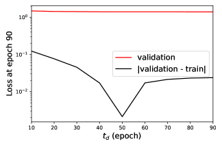
Figure 1: Validation loss and generalization error of SGDEM when training ResNet-18  (He et al., 2016) on ImageNet (Deng et al., 2009) in a distributed setting with 4 GPUs under tuned step-size and global minibatch size of 128. For each tdsubscript𝑡𝑑t_{d}, the momentum is set to μd=0.9subscript𝜇𝑑0.9\mu_{d}=0.9 in the first tdsubscript𝑡𝑑t_{d} epochs and then zero for the next 90td90subscript𝑡𝑑90-t_{d} epochs. SGDM is a special form of SGDEM with td=90subscript𝑡𝑑90t_{d}=90. The details are provided in Section 5 and Appendix L .

Stochastic gradient descent (SGD) and its variants are the most popular algorithms for training deep neural networks due to their support of efficient parallel implementations and excellent generalization performance (Krizhevsky et al., 2012; Wilson et al., 2017). To accelerate the convergence of SGD, a momentum term is often added in the iterative update of the stochastic gradient (Goodfellow et al., 2016). This approach has a long history, with proven benefits in various settings. The heavy-ball momentum method was first introduced by Polyak (1964) where a weighted version of the previous update is added to the current gradient update. Polyak (1964) motivated his method by its resemblance to a heavy ball moving in a potential well defined by the objective function. Momentum methods have been used to accelerate empirical risk minimization when training neural networks (Rumelhart et al., 1986). In particular, momentum methods are used for training deep neural networks with complex and nonconvex loss landscapes (Sutskever et al., 2013). Intuitively, adding momentum accelerates convergence by circumventing sharp curvatures and long ravines of the sub-level sets of the objective function (Wilson et al., 2021). Ochs et al. (2015) present an illustrative example to show that the momentum can potentially avoid local minima.

Beyond convergence, the generalization of machine learning algorithms is a fundamental problem in learning theory. A classical framework used to study the generalization error in machine learning is PAC learning (Vapnik and Chervonenkis, 1971; Valiant, 1984). However, the associated bounds using this approach can be conservative. The connection between stability and generalization has been studied in the literature, which captures how the learning algorithm explores a hypothesis class (Bousquet and Elisseeff, 2002; Shalev-Shwartz et al., 2010; Hardt et al., 2016). According to the definition of Bousquet and Elisseeff (2002), uniform stability requires the algorithm to generate almost the same predictions for all datasets that are different in only one example. Recently, this notion of uniform stability is leveraged to analyze the generalization error of SGD (Hardt et al., 2016). Hardt et al. (2016) have derived the stability bounds for SGD and analyzed its generalization for different loss functions. This is a substantial step forward, since SGD is widely used in many practical systems. However, the algorithms studied in these works do not include momentum.

In this work, we study SGD with momentum (SGDM). Although momentum methods are empirically observed to accelerate training in deep learning (Goodfellow et al., 2016), their effect on the generalization error is not well understood. Even though momentum is not studied in (Hardt et al., 2016), it is conjectured therein that momentum might speed up training but adversely impact generalization.

By providing a counter example, we show that the stability gap for multiple epochs of SGDM can become unbounded even for convex loss functions. This motivates us to consider a modified momentum-based update rule, called SGD with early momentum (SGDEM) where a momentum term is added in the earlier training steps. We show that SGDEM is guaranteed to generalize for smooth Lipschitz loss functions and any momentum. To the best of our knowledge, stability and generalization of SGDEM have not been considered in the existing literature. As Fig. 1 shows in a practical and distributed setting on ImageNet, while validation loss remains unaffected, the minimum generalization error happens if the momentum is applied for 50 epochs, which indicates that tuning momentum is useful to achieve the best generalization error.

We study the generalization error and true risk of SGDEM. In order to find an upper bound on the expected generalization error of SGDEM, we use the framework of uniform stability (Bousquet and Elisseeff, 2002; Hardt et al., 2016).

1.1 Main Contributions

In Section 3, we show that there exists a convex loss function for which the stability gap for multiple epochs of SGDM becomes unbounded. We introduce SGDEM and show that it is guaranteed to generalize for smooth Lipschitz loss functions. We obtain a bound on the generalization error of SGDEM that decreases inversely with the size of the training set. Our results show that the number of iterations can grow as nlsuperscript𝑛𝑙n^{l} for a small l>1𝑙1l>1 where n𝑛n is the sample size, which explains why complicated models such as deep neural networks can be trained for multiple epochs of SGDEM while their generalization errors are limited. We also establish an explicit convergence rate for SGDEM and smooth Lipschitz loss functions under a broad range of hyperparameters including a general step-size rule that covers popular step-sizes in the optimization literature. Our convergence and generalization bounds capture the inherent trade-off between optimization and generalization.

In Section 4, we focus on the special case of strongly convex loss functions. In this case, we show that one can obtain a bound on the generalization error of standard SGDM, which suggests that this special form of SGDEM suffices for generalization. Our bound is independent of the number of training iterations and decreases inversely with the size of the training set. Finally, we establish an upper bound on the expected true risk of SGDM as a function of various problem parameters.

Our generalization bounds for both strongly convex and smooth Lipschitz loss functions tend to zero as the number of samples increases. In addition, our results confirm that using a momentum parameter, μ1𝜇1\mu\approx 1, for the entire training improves optimization error under certain settings. However, it adversely affects the generalization error bounds. Hence, it is crucial to establish an appropriate balance between the optimization error associated with the empirical risk and the generalization error.

Finally, our experimental results show that SGDEM outperforms both vanilla SGD and SGDM in terms of test error on CIFAR10 and generalization error on ImageNet.

1.2 Related Work

Studies on the generalization of momentum methods are scarce in the literature. As explained above, momentum is not considered in (Bousquet and Elisseeff, 2002; Hardt et al., 2016). While the generalization error of SGDM is studied in (Ong, 2017) and (Chen et al., ), their analysis is limited to the special case of quadratic loss functions. In this work, we show that unlike SGDM, multiple epochs of SGDEM is guaranteed to generalize for smooth Lipschitz loss functions. A similar hybrid method has been shown to generalize better than both vanilla SGD and Adaptive Moment Estimation (Adam) in deep learning practice (Keskar and Socher, ). However, it remains unclear why such hybrid methods generalize better. Our work sheds theoretical light on this question.

Convergence of first-order methods with momentum has been studied in (Polyak, 1964; Ochs et al., 2014, 2015; Ghadimi et al., 2015; Lessard et al., 2016; Yan et al., 2018; Wilson et al., 2021; Gadat et al., 2018; Orvieto et al., 2020; Can et al., 2019). Most of these works consider the deterministic setting for gradient update (Polyak, 1964; Ochs et al., 2014, 2015; Ghadimi et al., 2015; Lessard et al., 2016; Wilson et al., 2021). Only a few works have analyzed convergence in the stochastic setting (Yan et al., 2018; Gadat et al., 2018; Orvieto et al., 2020; Can et al., 2019). In (Yan et al., 2018), a unified convergence analysis of SGDM has been studied for both convex and nonconvex loss functions with bounded variance. Gadat et al. (2018) have studied the almost sure convergence results of the stochastic heavy-ball method with nonconvex coercive loss functions and provided a complexity analysis for the case of quadratic strongly convex. In (Orvieto et al., 2020), differential equation-based analysis is used to study convergence of SGDM. Can et al. (2019) have obtained linear convergence rates for SGDM under a particular momentum for the special case of quadratic loss functions. In this paper, we introduce early momentum for the class of smooth Lipschitz loss functions, which requires unique convergence analysis as shown in Section 3.

We further note that Lessard et al. (2016) have provided a specific loss function for which the heavy-ball method does not converge. This loss function does not contradict our convergence analysis. The loss function in (Lessard et al., 2016) has been carefully constructed and does not satisfy the assumptions considered in this paper.

In addition to Polyak’s heavy-ball momentum method, Nesterov (1983) has proposed an accelerated gradient descent, which converges as O(1/k2)𝑂1superscript𝑘2O(1/k^{2}) in a deterministic and convex setting where k𝑘k is the number of iterations. Convergence rates are obtained for Nesterov’s accelerated gradient method in various settings (Su et al., 2014; Laborde and Oberman, 2020; Assran and Rabbat, 2020). However, the Netstrov momentum does not seem to improve the rate of convergence for stochastic gradient settings (Goodfellow et al., 2016, Section 8.3.3). Therefore, in this work we focus on the heavy-ball momentum.

High-probability bounds on the generalization error of uniformly stable algorithms over the random choice of the dataset have been recently established in (Feldman and Vondrak, 2018, 2019; Bousquet et al., 2020; Klochkov and Zhivotovskiy, 2021). Momentum-based methods have not been considered in these works. In this paper, we establish generalization errors for momentum-based methods with a focus on the randomness of the algorithm.

Our results complement the recent results of Attia and Koren (2021), which show exponential growth in uniform stability bounds of accelerated gradient descent methods. We focus on stochastic gradient descent with heavy-ball momentum for possibly nonconvex problems under nonconstant step-sizes, while Attia and Koren (2021) focus on convex problems with full-batch Nesterov’s accelerated gradient under a fixed step-size.

Notation: We use 𝔼[]𝔼delimited-[]\mathbb{E}[\cdot] to denote the expectation and \|\cdot\| to represent the Euclidean norm of a vector. We use lower-case bold font to denote vectors. We use sans-serif font to denote random quantities. Sets and scalars are represented by calligraphic and standard fonts, respectively.

2 Problem and Assumptions

We consider a general supervised learning problem, where 𝒮={𝘇1,,𝘇n}𝒮subscript𝘇1subscript𝘇𝑛{\cal S}=\{{\bm{\mathsf{z}}}_{1},\ldots,{\bm{\mathsf{z}}}_{n}\} denotes the set of samples of size n𝑛n drawn i.i.d. from some space 𝒵𝒵{\cal Z} with an unknown distribution D𝐷D. We assume a learning model described by parameter vector 𝐰Ω𝐰Ω{\bf w}\in\Omega. Let (𝐰;𝐳)𝐰𝐳\ell({\bf w};{\bf z}) denote the loss of the model described by parameter 𝐰𝐰{\bf w} on example 𝐳𝒵𝐳𝒵{\bf z}\in{\cal Z}.

The ultimate goal of learning is to minimize the true or population risk given by

R(𝐰):=𝔼𝘇D[(𝐰;𝘇)].assign𝑅𝐰subscript𝔼similar-to𝘇𝐷delimited-[]𝐰𝘇\displaystyle R({\bf w}):=\mathbb{E}_{{\bm{\mathsf{z}}}\sim D}[\ell({\bf w};{\bm{\mathsf{z}}})]. (2.1)

Since the distribution D𝐷D is unknown, we approximate this objective by the empirical risk during training, i.e.,R𝒮(𝐰):=1ni=1n(𝐰;𝘇i){\it i.e.,\ \/}R_{\cal S}({\bf w}):=\frac{1}{n}\sum_{i=1}^{n}\ell({\bf w};{\bm{\mathsf{z}}}_{i}). We assume 𝘄=A(𝒮)𝘄𝐴𝒮{\bm{\mathsf{w}}}=A({\cal S}) for some potentially randomized algorithm A𝐴A.

2.1 Generalization Error and Stability

In order to find an upper bound on the true risk of algorithm A𝐴A, in this work, we consider the generalization error, which is the expected difference of empirical and true risk:

ϵg:=𝔼𝒮,A[R(A(𝒮))R𝒮(A(𝒮))].assignsubscriptitalic-ϵ𝑔subscript𝔼𝒮𝐴delimited-[]𝑅𝐴𝒮subscript𝑅𝒮𝐴𝒮\displaystyle\epsilon_{g}:=\mathbb{E}_{{\cal S},A}[R(A({\cal S}))-R_{\cal S}(A({\cal S}))]. (2.2)

In order to find an upper bound on the generalization error of algorithm A𝐴A, we consider the uniform stability property.

Definition 1

Let 𝒮𝒮{\cal S} and 𝒮superscript𝒮{\cal S}^{\prime} denote two datasets from space 𝒵nsuperscript𝒵𝑛{\cal Z}^{n} such that 𝒮𝒮{\cal S} and 𝒮superscript𝒮{\cal S}^{\prime} differ in at most one example. Algorithm A𝐴A is ϵssubscriptitalic-ϵ𝑠\epsilon_{s}-uniformly stable if for all datasets 𝒮𝒮{\cal S} and 𝒮superscript𝒮{\cal S}^{\prime}, we have

sup𝐳𝔼A[(A(𝒮);𝐳)(A(𝒮);𝐳)]ϵs.subscriptsupremum𝐳subscript𝔼𝐴delimited-[]𝐴𝒮𝐳𝐴superscript𝒮𝐳subscriptitalic-ϵ𝑠\displaystyle\sup_{\bf z}\mathbb{E}_{A}[\ell(A({\cal S});{\bf z})-\ell(A({\cal S}^{\prime});{\bf z})]\leq\epsilon_{s}. (2.3)

It is known that uniform stability implies generalization in expectation:

Theorem 2 (Hardt et al. 2016)

If A𝐴A is an ϵssubscriptitalic-ϵ𝑠\epsilon_{s}-uniformly stable algorithm, then the generalization error of A𝐴A is upper bounded by ϵssubscriptitalic-ϵ𝑠\epsilon_{s}.

Theorem 2 suggests that it is enough to control the uniform stability of an algorithm to bound the generalization error.

2.2 SGDM

The update rule for SGDM is given by

𝘄t+1subscript𝘄𝑡1\displaystyle{{\bm{\mathsf{w}}}}_{t+1} =𝘄t+μ(𝘄t𝘄t1)αt𝐰(𝘄t;𝐳𝗂t)absentsubscript𝘄𝑡𝜇subscript𝘄𝑡subscript𝘄𝑡1subscript𝛼𝑡subscript𝐰subscript𝘄𝑡subscript𝐳subscript𝗂𝑡\displaystyle={\bm{\mathsf{w}}}_{t}+\mu({\bm{\mathsf{w}}}_{t}-{\bm{\mathsf{w}}}_{t-1})-\alpha_{t}\nabla_{\bf w}\ell({\bm{\mathsf{w}}}_{t};{\bf z}_{{\mathsf{i}}_{t}}) (SGDM)

where αt>0subscript𝛼𝑡0\alpha_{t}>0 is the step-size, μ(0,1]𝜇01\mu\in(0,1] is the momentum parameter, 𝗂t{1,,n}subscript𝗂𝑡1𝑛{\mathsf{i}}_{t}\in\{1,\ldots,n\} is a selected index drawn uniformly at random at each iteration, and (𝘄t;𝐳𝗂t)subscript𝘄𝑡subscript𝐳subscript𝗂𝑡\ell({\bm{\mathsf{w}}}_{t};{\bf z}_{{\mathsf{i}}_{t}}) is the loss evaluated on sample 𝐳𝗂tsubscript𝐳subscript𝗂𝑡{\bf z}_{{\mathsf{i}}_{t}}.111Another variant to select 𝗂tsubscript𝗂𝑡{\mathsf{i}}_{t} is to permutate {1,,n}1𝑛\{1,\ldots,n\} randomly once and then select the examples repeatedly in a cyclic manner. Our stability analysis in Sections 3.2 and 4 holds under both variants, i.e., uniformly at random with replacement and random permutation. In SGDM, we run the update iteratively for T𝑇T steps and let 𝘄Tsubscript𝘄𝑇{\bm{\mathsf{w}}}_{T} denote the final output.

In the case where the parameter space ΩΩ\Omega is a compact and convex set, we consider the update rule for projected SGDM:

𝘄t+1subscript𝘄𝑡1\displaystyle{{\bm{\mathsf{w}}}}_{t+1} =𝐏(𝘄t+μ(𝘄t𝘄t1)αt𝐰(𝘄t;𝐳𝗂t))absent𝐏subscript𝘄𝑡𝜇subscript𝘄𝑡subscript𝘄𝑡1subscript𝛼𝑡subscript𝐰subscript𝘄𝑡subscript𝐳subscript𝗂𝑡\displaystyle={\bf P}\Big{(}{\bm{\mathsf{w}}}_{t}+\mu({\bm{\mathsf{w}}}_{t}-{\bm{\mathsf{w}}}_{t-1})-\alpha_{t}\nabla_{\bf w}\ell({\bm{\mathsf{w}}}_{t};{\bf z}_{{\mathsf{i}}_{t}})\Big{)} (P-SGDM)

where 𝐏𝐏{\bf P} denotes the Euclidean projection onto ΩΩ\Omega. The key quantity of interest in this paper is the generalization error given by

ϵg=𝔼𝒮,A[R(𝘄T)R𝒮(𝘄T)]=𝔼𝒮,𝗂0,,𝗂T1[R(𝘄T)R𝒮(𝘄T)]subscriptitalic-ϵ𝑔subscript𝔼𝒮𝐴delimited-[]𝑅subscript𝘄𝑇subscript𝑅𝒮subscript𝘄𝑇subscript𝔼𝒮subscript𝗂0subscript𝗂𝑇1delimited-[]𝑅subscript𝘄𝑇subscript𝑅𝒮subscript𝘄𝑇\displaystyle\epsilon_{g}=\mathbb{E}_{{\cal S},A}[R({\bm{\mathsf{w}}}_{T})-R_{\cal S}({\bm{\mathsf{w}}}_{T})]=\mathbb{E}_{{\cal S},{\mathsf{i}}_{0},\ldots,{\mathsf{i}}_{T-1}}[R({\bm{\mathsf{w}}}_{T})-R_{\cal S}({\bm{\mathsf{w}}}_{T})]

since the randomness in A𝐴A arises from the choice of 𝗂0,,𝗂T1subscript𝗂0subscript𝗂𝑇1{\mathsf{i}}_{0},\ldots,{\mathsf{i}}_{T-1}.

2.3 Assumptions on Loss Function

Let 𝐳𝒵𝐳𝒵{\bf z}\in{\cal Z}. In our analysis, we will assume that the loss function (;𝐳)𝐳\ell(\cdot;{\bf z}) satisfies the following properties, which are used also in (Hardt et al., 2016).

Assumption 1 (Lipschitzness & smoothness)

Let 𝐳𝒵𝐳𝒵{\bf z}\in{\cal Z}. The loss function (;𝐳)𝐳\ell(\cdot;{\bf z}) satisfies the following properties: 1) L𝐿L-Lipschitzness: There exists some L>0𝐿0L>0 such that |(𝐮;𝐳)(𝐯;𝐳)|L𝐮𝐯𝐮𝐳𝐯𝐳𝐿norm𝐮𝐯|\ell({\bf u};{\bf z})-\ell({\bf v};{\bf z})|\leq L\|{\bf u}-{\bf v}\| for all 𝐮,𝐯Ω𝐮𝐯Ω{\bf u},{\bf v}\in\Omega; 2) β𝛽\beta-smoothness: There exists some β>0𝛽0\beta>0 such that (𝐮;𝐳)(𝐯;𝐳)β𝐮𝐯norm𝐮𝐳𝐯𝐳𝛽norm𝐮𝐯\|\nabla\ell({\bf u};{\bf z})-\nabla\ell({\bf v};{\bf z})\|\leq\beta\|{\bf u}-{\bf v}\| for all 𝐮,𝐯Ω𝐮𝐯Ω{\bf u},{\bf v}\in\Omega.

Our assumptions hold for neural networks with smooth activation functions such as smooth approximations of ReLU including softplus or Gaussian error Linear Units (GeLU) (Dugas et al., 2000; Hendrycks and Gimpel, ). We note that softplus and GeLU typically match and exceed performance compared to ReLU (Clevert et al., 2016; Xu et al., ).

3 Smooth Lipschitz Loss

We first show that there exists a convex loss function for which the stability gap for multiple epochs of SGDM becomes unbounded. For the case of smooth Lipschitz loss functions, we introduce SGDEM and show that machine learning models can be trained for multiple epochs of SGDEM while their generalization errors are bounded.

In SGDEM, the momentum μ𝜇\mu is set to some constant μd(0,1]subscript𝜇𝑑01\mu_{d}\in(0,1] in the first tdsubscript𝑡𝑑t_{d} steps and then zero for t=td+1,,T𝑡subscript𝑡𝑑1𝑇t=t_{d}+1,\ldots,T. Thus, the update rule for SGDEM is given by

𝘄t+1subscript𝘄𝑡1\displaystyle{{\bm{\mathsf{w}}}}_{t+1} =𝘄t+μd𝟙(ttd)(𝘄t𝘄t1)αt𝐰(𝘄t;𝐳𝗂t)absentsubscript𝘄𝑡subscript𝜇𝑑1𝑡subscript𝑡𝑑subscript𝘄𝑡subscript𝘄𝑡1subscript𝛼𝑡subscript𝐰subscript𝘄𝑡subscript𝐳subscript𝗂𝑡\displaystyle={\bm{\mathsf{w}}}_{t}+\mu_{d}\mathbbm{1}(t\leq t_{d})({\bm{\mathsf{w}}}_{t}-{\bm{\mathsf{w}}}_{t-1})-\alpha_{t}\nabla_{\bf w}\ell({\bm{\mathsf{w}}}_{t};{\bf z}_{{\mathsf{i}}_{t}}) (SGDEM)

where 𝟙1\mathbbm{1} denotes the indicator function, and the projected version can be similarly defined based on P-SGDM.

3.1 Uniform Stability Bounds for SGDM and SGDEM

Example 1

Let w[1,1]𝑤11w\in[-1,1] denote a parameter. Consider the one-dimensional and convex loss function (w;𝐳)=L𝐳w+c𝐳𝑤𝐳subscript𝐿𝐳𝑤subscript𝑐𝐳\ell(w;{\bf z})=L_{{\bf z}}w+c_{{\bf z}} where L𝐳{L,L}subscript𝐿𝐳𝐿𝐿L_{{\bf z}}\in\{L,-L\} depending on 𝐳𝒵𝐳𝒵{\bf z}\in{\cal Z} and c𝐳0subscript𝑐𝐳0c_{{\bf z}}\geq 0 is constant w.r.t. w𝑤w. For a specific choice of 𝒮𝒮{\cal S} with

R𝒮(w)=1ni=1n(Lw+ci)=Lw+i=1ncin,subscript𝑅𝒮𝑤1𝑛superscriptsubscript𝑖1𝑛𝐿𝑤subscript𝑐𝑖𝐿𝑤superscriptsubscript𝑖1𝑛subscript𝑐𝑖𝑛\displaystyle R_{{\cal S}}(w)=\frac{1}{n}\sum_{i=1}^{n}(Lw+c_{i})=Lw+\sum_{i=1}^{n}\frac{c_{i}}{n},

the optimal parameter minimizing the empirical risk is w𝒮=1subscriptsuperscript𝑤𝒮1w^{*}_{{\cal S}}=-1.

Both SGDM and SGDEM can find the optimal solution of our convex empirical risk minimization problem. We first establish a lower bound on the stability gap when SGDM is run for multiple epochs, which shows that the gap can be unbounded.222If we set T=nl𝑇superscript𝑛𝑙T=n^{l} for some l>1𝑙1l>1, the stability gap will become unbounded as n𝑛n\rightarrow\infty regardless of μ𝜇\mu. If we set T=kn𝑇𝑘𝑛T=kn with k>1𝑘1k>1, there will still be a nonvanishing gap regardless of μ𝜇\mu (the gap does not blow up but it does not vanish). In our analysis of the stability, our goal is to track the divergence of two different iterative sequences of update rules with the same starting point.

Theorem 3

Let 𝐳𝒵𝐳𝒵{\bf z}\in{\cal Z}. Suppose that the SGDM update is executed for T𝑇T steps with constant step-size α>0𝛼0\alpha>0 and μ(0,1]𝜇01\mu\in(0,1] on Example 1. There exist datasets 𝒮𝒮{\cal S} and 𝒮superscript𝒮{\cal S}^{\prime} such that 𝔼A[(A(𝒮);𝐳)(A(𝒮);𝐳)]subscript𝔼𝐴delimited-[]𝐴𝒮𝐳𝐴superscript𝒮𝐳\mathbb{E}_{A}[\ell(A({\cal S});{\bf z})-\ell(A({\cal S}^{\prime});{\bf z})] is lower bounded by Ω(Tn(1+kμk))Ω𝑇𝑛1𝑘superscript𝜇𝑘\Omega(\frac{T}{n}(1+k\mu^{k})) with k=log(T)𝑘𝑇k=\lceil\log(T)\rceil.333 We note that the lower bound in Theorem 3 matches an upper bound for SGD with smooth and convex losses, and early-stopped SGDM will be stable by setting T𝑇T sublinearly in n𝑛n.

Proof We consider two neighbouring datasets 𝒮𝒮{\cal S} and 𝒮superscript𝒮{\cal S}^{\prime} with

R𝒮(w)=1ni=1n(Lw+ci)=Lw+c¯subscript𝑅𝒮𝑤1𝑛superscriptsubscript𝑖1𝑛𝐿𝑤subscript𝑐𝑖𝐿𝑤¯𝑐\displaystyle R_{{\cal S}}(w)=\frac{1}{n}\sum_{i=1}^{n}(Lw+c_{i})=Lw+\overline{c}

and

R𝒮(w)=1nLw+ckn+1ni=1,ikn(Lw+ci)=n2nLw+ckckn+c¯subscript𝑅superscript𝒮𝑤1𝑛𝐿𝑤subscriptsuperscript𝑐𝑘𝑛1𝑛superscriptsubscriptformulae-sequence𝑖1𝑖𝑘𝑛𝐿𝑤subscript𝑐𝑖𝑛2𝑛𝐿𝑤subscriptsuperscript𝑐𝑘subscript𝑐𝑘𝑛¯𝑐\displaystyle R_{{\cal S}^{\prime}}(w)=-\frac{1}{n}Lw+\frac{c^{\prime}_{k}}{n}+\frac{1}{n}\sum_{i=1,i\neq k}^{n}(Lw+c_{i})=\frac{n-2}{n}Lw+\frac{c^{\prime}_{k}-c_{k}}{n}+\overline{c}

where c¯=1ni=1nci¯𝑐1𝑛superscriptsubscript𝑖1𝑛subscript𝑐𝑖\overline{c}=\frac{1}{n}\sum_{i=1}^{n}c_{i}. Suppose we select an index 𝗂tsubscript𝗂𝑡{\mathsf{i}}_{t} uniformly at random from {1,,n}1𝑛\{1,\ldots,n\}. Then we have 𝔼𝗂t[(w;𝐳𝗂t)]=R𝒮(w)=Lsubscript𝔼subscript𝗂𝑡delimited-[]𝑤subscript𝐳subscript𝗂𝑡subscript𝑅𝒮𝑤𝐿\mathbb{E}_{{\mathsf{i}}_{t}}[\nabla\ell(w;{\bf z}_{{\mathsf{i}}_{t}})]=\nabla R_{{\cal S}}(w)=L and 𝔼𝗂t[(w;𝐳𝗂t)]=R𝒮(w)=(n2)L/nsubscript𝔼subscript𝗂𝑡delimited-[]𝑤subscriptsuperscript𝐳subscript𝗂𝑡subscript𝑅superscript𝒮𝑤𝑛2𝐿𝑛\mathbb{E}_{{\mathsf{i}}_{t}}[\nabla\ell(w;{\bf z}^{\prime}_{{\mathsf{i}}_{t}})]=\nabla R_{{\cal S}^{\prime}}(w)=(n-2)L/n, which holds for all wΩ𝑤Ωw\in\Omega. Let 𝗐Tsubscript𝗐𝑇{\mathsf{w}}_{T} and 𝗐Tsubscriptsuperscript𝗐𝑇{\mathsf{w}}^{\prime}_{T} denote the outputs of SGDM on 𝒮𝒮{\cal S} and 𝒮superscript𝒮{\cal S}^{\prime}, respectively. Suppose 𝗐0=𝗐0subscript𝗐0subscriptsuperscript𝗐0{\mathsf{w}}_{0}={\mathsf{w}}^{\prime}_{0}. We can follow the steps of SGDM on 𝒮𝒮{\cal S} and obtain444We assume 𝗐0,α,μsubscript𝗐0𝛼𝜇{\mathsf{w}}_{0},\alpha,\mu are set such that the updated parameter remains in the parameter space.

𝔼𝗂0,,𝗂T1[𝗐T]=(T+(T1)μ+(T2)μ2++μT1)αL+𝔼[𝗐0].subscript𝔼subscript𝗂0subscript𝗂𝑇1delimited-[]subscript𝗐𝑇𝑇𝑇1𝜇𝑇2superscript𝜇2superscript𝜇𝑇1𝛼𝐿𝔼delimited-[]subscript𝗐0\displaystyle\mathbb{E}_{{\mathsf{i}}_{0},\ldots,{\mathsf{i}}_{T-1}}[{\mathsf{w}}_{T}]=-(T+(T-1)\mu+(T-2)\mu^{2}+\cdots+\mu^{T-1})\alpha L+\mathbb{E}[{\mathsf{w}}_{0}].

Similarly, we have

𝔼𝗂0,,𝗂T1[𝗐T]=(T+(T1)μ+(T2)μ2++μT1)(n2)αLn+𝔼[𝗐0].subscript𝔼subscript𝗂0subscript𝗂𝑇1delimited-[]subscriptsuperscript𝗐𝑇𝑇𝑇1𝜇𝑇2superscript𝜇2superscript𝜇𝑇1𝑛2𝛼𝐿𝑛𝔼delimited-[]subscript𝗐0\displaystyle\mathbb{E}_{{\mathsf{i}}_{0},\ldots,{\mathsf{i}}_{T-1}}[{\mathsf{w}}^{\prime}_{T}]=-(T+(T-1)\mu+(T-2)\mu^{2}+\cdots+\mu^{T-1})\frac{(n-2)\alpha L}{n}+\mathbb{E}[{\mathsf{w}}_{0}].

Hence, we have

𝔼A[𝗐T𝗐T]=2αLn(T+(T1)μ+(T2)μ2++μT1).subscript𝔼𝐴delimited-[]subscriptsuperscript𝗐𝑇subscript𝗐𝑇2𝛼𝐿𝑛𝑇𝑇1𝜇𝑇2superscript𝜇2superscript𝜇𝑇1\mathbb{E}_{A}[{\mathsf{w}}^{\prime}_{T}-{\mathsf{w}}_{T}]=\frac{2\alpha L}{n}(T+(T-1)\mu+(T-2)\mu^{2}+\cdots+\mu^{T-1}).

Let 𝐳𝒵𝐳𝒵{\bf z}\in{\cal Z}. Using Jensen’s inequality, we can show that

𝔼A[|(𝗐T;𝐳)(𝗐T;𝐳)|]subscript𝔼𝐴delimited-[]subscript𝗐𝑇𝐳subscriptsuperscript𝗐𝑇𝐳\displaystyle\mathbb{E}_{A}[|\ell({\mathsf{w}}_{T};{\bf z})-\ell({\mathsf{w}}^{\prime}_{T};{\bf z})|] |𝔼A[(𝗐T;𝐳)(𝗐T;𝐳)]|absentsubscript𝔼𝐴delimited-[]subscript𝗐𝑇𝐳subscriptsuperscript𝗐𝑇𝐳\displaystyle\geq|\mathbb{E}_{A}[\ell({\mathsf{w}}_{T};{\bf z})-\ell({\mathsf{w}}^{\prime}_{T};{\bf z})]|
=2αL2nj=0T1(Tj)μj.absent2𝛼superscript𝐿2𝑛superscriptsubscript𝑗0𝑇1𝑇𝑗superscript𝜇𝑗\displaystyle=\frac{2\alpha L^{2}}{n}\sum_{j=0}^{T-1}(T-j)\mu^{j}.

Hence, 𝔼A[|(𝗐T;𝐳)(𝗐T;𝐳)|]subscript𝔼𝐴delimited-[]subscript𝗐𝑇𝐳subscriptsuperscript𝗐𝑇𝐳\mathbb{E}_{A}[|\ell({\mathsf{w}}_{T};{\bf z})-\ell({\mathsf{w}}^{\prime}_{T};{\bf z})|] is lower bounded by Ω(T/n(1+kμk))Ω𝑇𝑛1𝑘superscript𝜇𝑘\Omega(T/n(1+k\mu^{k})) where k=o(T)𝑘𝑜𝑇k=o(T).  

Note that the stability lower bound increases monotonically with μ𝜇\mu. For the same example, we can show that the stability gap for multiple epochs of SGDEM goes to zero.

Theorem 4

Let μd(0,1)subscript𝜇𝑑01\mu_{d}\in(0,1). For Example 1 and datasets described in Theorem 3, the stability gap for SGDEM and SGDM goes to zero as n𝑛n\to\infty as long as j=1Tαj=o(n)superscriptsubscript𝑗1𝑇subscript𝛼𝑗𝑜𝑛\sum_{j=1}^{T}\alpha_{j}=o(n).

Furthermore, under T=nl𝑇superscript𝑛𝑙T=n^{l} with some l>1𝑙1l>1 and td(j=1Tαj2)1/3=o(T23l)subscript𝑡𝑑superscriptsuperscriptsubscript𝑗1𝑇superscriptsubscript𝛼𝑗213𝑜superscript𝑇23𝑙t_{d}\big{(}\sum_{j=1}^{T}\alpha_{j}^{2}\big{)}^{1/3}=o(T^{\frac{2}{3l}}), the stability gap for SGDEM goes to zero for any μd(0,1]subscript𝜇𝑑01\mu_{d}\in(0,1].

Proof Let 𝗐Tsubscript𝗐𝑇{\mathsf{w}}_{T} and 𝗐Tsubscriptsuperscript𝗐𝑇{\mathsf{w}}^{\prime}_{T} denote the outputs of SGDEM on 𝒮𝒮{\cal S} and 𝒮superscript𝒮{\cal S}^{\prime}, respectively. Following the steps of SGDEM on 𝒮𝒮{\cal S}, we have

𝔼𝗂0,,𝗂T1[𝗐T]subscript𝔼subscript𝗂0subscript𝗂𝑇1delimited-[]subscript𝗐𝑇\displaystyle\mathbb{E}_{{\mathsf{i}}_{0},\ldots,{\mathsf{i}}_{T-1}}[{\mathsf{w}}_{T}] =L(α1++αT)α1L(μd++μdtd1)α2L2(μd++μdtd2)absent𝐿subscript𝛼1subscript𝛼𝑇subscript𝛼1𝐿subscript𝜇𝑑superscriptsubscript𝜇𝑑subscript𝑡𝑑1subscript𝛼2superscript𝐿2subscript𝜇𝑑superscriptsubscript𝜇𝑑subscript𝑡𝑑2\displaystyle=-L(\alpha_{1}+\cdots+\alpha_{T})-\alpha_{1}L(\mu_{d}+\cdots+\mu_{d}^{t_{d}-1})-\alpha_{2}L^{2}(\mu_{d}+\cdots+\mu_{d}^{t_{d}-2})
αtd1Lμd+𝔼[𝗐0].subscript𝛼subscript𝑡𝑑1𝐿subscript𝜇𝑑𝔼delimited-[]subscript𝗐0\displaystyle\quad-\cdots-\alpha_{t_{d}-1}L\mu_{d}+\mathbb{E}[{\mathsf{w}}_{0}].

Similarly, we have

E𝗂0,,𝗂T1[𝗐T]subscript𝐸subscript𝗂0subscript𝗂𝑇1delimited-[]subscriptsuperscript𝗐𝑇\displaystyle E_{{\mathsf{i}}_{0},\ldots,{\mathsf{i}}_{T-1}}[{\mathsf{w}}^{\prime}_{T}] =((n2)/n)L(α1++αT)((n2)/n)α1L(μd++μdtd1)absent𝑛2𝑛𝐿subscript𝛼1subscript𝛼𝑇𝑛2𝑛subscript𝛼1𝐿subscript𝜇𝑑superscriptsubscript𝜇𝑑subscript𝑡𝑑1\displaystyle=-((n-2)/n)L(\alpha_{1}+\cdots+\alpha_{T})-((n-2)/n)\alpha_{1}L(\mu_{d}+\cdots+\mu_{d}^{t_{d}-1})
((n2)/n)α2L2(μd++μdtd2)((n2)/n)αtd1Lμd+𝔼[𝗐0].𝑛2𝑛subscript𝛼2superscript𝐿2subscript𝜇𝑑superscriptsubscript𝜇𝑑subscript𝑡𝑑2𝑛2𝑛subscript𝛼subscript𝑡𝑑1𝐿subscript𝜇𝑑𝔼delimited-[]subscript𝗐0\displaystyle\quad-((n-2)/n)\alpha_{2}L^{2}(\mu_{d}+\cdots+\mu_{d}^{t_{d}-2})-\cdots-((n-2)/n)\alpha_{t_{d}-1}L\mu_{d}+\mathbb{E}[{\mathsf{w}}_{0}].

Let 𝐳𝒵𝐳𝒵{\bf z}\in{\cal Z}. For this particular example, we have 𝔼A[|(𝗐T;𝐳)(𝗐T;𝐳)|]=L𝔼A|𝗐T𝗐T|.subscript𝔼𝐴delimited-[]subscript𝗐𝑇𝐳subscriptsuperscript𝗐𝑇𝐳𝐿subscript𝔼𝐴subscript𝗐𝑇subscriptsuperscript𝗐𝑇\mathbb{E}_{A}[|\ell({\mathsf{w}}_{T};{\bf z})-\ell({\mathsf{w}}^{\prime}_{T};{\bf z})|]=L\mathbb{E}_{A}|{\mathsf{w}}_{T}-{\mathsf{w}}^{\prime}_{T}|.

Lemma 5

𝗐T𝗐T0subscriptsuperscript𝗐𝑇subscript𝗐𝑇0{\mathsf{w}}^{\prime}_{T}-{\mathsf{w}}_{T}\geq 0 everywhere.

Proof Let wTsubscript𝑤𝑇w_{T} and wTsuperscriptsubscript𝑤𝑇w_{T}^{\prime} denote a realization of 𝗐Tsubscript𝗐𝑇{\mathsf{w}}_{T} and 𝗐Tsubscriptsuperscript𝗐𝑇{\mathsf{w}}^{\prime}_{T}, respectively. Let w0subscript𝑤0w_{0} denote a realization of 𝗐0subscript𝗐0{\mathsf{w}}_{0}, and fix (𝗂0,,𝗂T1)subscript𝗂0subscript𝗂𝑇1({\mathsf{i}}_{0},\ldots,{\mathsf{i}}_{T-1}) where the differing index between 𝒮𝒮{\cal S} and 𝒮superscript𝒮{\cal S}^{\prime} happens at steps in 𝒥={j1,,jm}𝒥subscript𝑗1subscript𝑗𝑚{\cal J}=\{j_{1},\ldots,j_{m}\}. Then we have

wTsubscript𝑤𝑇\displaystyle w_{T} =L(α1++αT)α1L(μd++μdtd1)α2L2(μd++μdtd2)absent𝐿subscript𝛼1subscript𝛼𝑇subscript𝛼1𝐿subscript𝜇𝑑superscriptsubscript𝜇𝑑subscript𝑡𝑑1subscript𝛼2superscript𝐿2subscript𝜇𝑑superscriptsubscript𝜇𝑑subscript𝑡𝑑2\displaystyle=-L(\alpha_{1}+\cdots+\alpha_{T})-\alpha_{1}L(\mu_{d}+\cdots+\mu_{d}^{t_{d}-1})-\alpha_{2}L^{2}(\mu_{d}+\cdots+\mu_{d}^{t_{d}-2})
αtd1Lμd+w0subscript𝛼subscript𝑡𝑑1𝐿subscript𝜇𝑑subscript𝑤0\displaystyle\quad-\cdots-\alpha_{t_{d}-1}L\mu_{d}+w_{0}

and

wTsuperscriptsubscript𝑤𝑇\displaystyle w_{T}^{\prime} =Lj𝒯/𝒥αj+Lj𝒥αjLj𝒯d/𝒥dαj(μd++μdtdj)absent𝐿subscript𝑗𝒯𝒥subscript𝛼𝑗𝐿subscript𝑗𝒥subscript𝛼𝑗𝐿subscript𝑗subscript𝒯𝑑subscript𝒥𝑑subscript𝛼𝑗subscript𝜇𝑑superscriptsubscript𝜇𝑑subscript𝑡𝑑𝑗\displaystyle=-L\sum_{j\in{\cal T}/{\cal J}}\alpha_{j}+L\sum_{j\in{\cal J}}\alpha_{j}-L\sum_{j\in{\cal T}_{d}/{\cal J}_{d}}\alpha_{j}(\mu_{d}+\cdots+\mu_{d}^{t_{d}-j})
+Lj𝒥dαj(μd++μdtdj)+w0𝐿subscript𝑗subscript𝒥𝑑subscript𝛼𝑗subscript𝜇𝑑superscriptsubscript𝜇𝑑subscript𝑡𝑑𝑗subscript𝑤0\displaystyle\quad+L\sum_{j\in{\cal J}_{d}}\alpha_{j}(\mu_{d}+\cdots+\mu_{d}^{t_{d}-j})+w_{0}

where 𝒯={1,,T}𝒯1𝑇{\cal T}=\{1,\ldots,T\}, 𝒯d={1,,td}subscript𝒯𝑑1subscript𝑡𝑑{\cal T}_{d}=\{1,\ldots,t_{d}\}, and 𝒥d={j𝒥:jtd}subscript𝒥𝑑conditional-set𝑗𝒥𝑗subscript𝑡𝑑{\cal J}_{d}=\{j\in{\cal J}:\leavevmode\nobreak\ j\leq t_{d}\}. This shows wTwTsuperscriptsubscript𝑤𝑇subscript𝑤𝑇w_{T}^{\prime}\geq w_{T}. We note that the set of realizations with wT<wTsuperscriptsubscript𝑤𝑇subscript𝑤𝑇w_{T}^{\prime}<w_{T} is empty.  
This lemma shows 𝔼A|𝗐T𝗐T|=𝔼A[𝗐T]𝔼A[𝗐T]subscript𝔼𝐴subscript𝗐𝑇subscriptsuperscript𝗐𝑇subscript𝔼𝐴delimited-[]subscriptsuperscript𝗐𝑇subscript𝔼𝐴delimited-[]subscript𝗐𝑇\mathbb{E}_{A}|{\mathsf{w}}_{T}-{\mathsf{w}}^{\prime}_{T}|=\mathbb{E}_{A}[{\mathsf{w}}^{\prime}_{T}]-\mathbb{E}_{A}[{\mathsf{w}}_{T}]. We first note that

𝔼A[|(𝗐T;𝐳)(𝗐T;𝐳)|]=2L2nj=1Tαj+2L2nj=1tdαj(μd++μdtdj)2L2nj=1Tαj+2L2μdn(1μd)j=1tdαj2L2j=1Tαjn(1+μd1μd).subscript𝔼𝐴delimited-[]subscript𝗐𝑇𝐳subscriptsuperscript𝗐𝑇𝐳2superscript𝐿2𝑛superscriptsubscript𝑗1𝑇subscript𝛼𝑗2superscript𝐿2𝑛superscriptsubscript𝑗1subscript𝑡𝑑subscript𝛼𝑗subscript𝜇𝑑superscriptsubscript𝜇𝑑subscript𝑡𝑑𝑗2superscript𝐿2𝑛superscriptsubscript𝑗1𝑇subscript𝛼𝑗2superscript𝐿2subscript𝜇𝑑𝑛1subscript𝜇𝑑superscriptsubscript𝑗1subscript𝑡𝑑subscript𝛼𝑗2superscript𝐿2superscriptsubscript𝑗1𝑇subscript𝛼𝑗𝑛1subscript𝜇𝑑1subscript𝜇𝑑\displaystyle\begin{split}\mathbb{E}_{A}[|\ell({\mathsf{w}}_{T};{\bf z})-\ell({\mathsf{w}}^{\prime}_{T};{\bf z})|]&=\frac{2L^{2}}{n}\sum_{j=1}^{T}\alpha_{j}+\frac{2L^{2}}{n}\sum_{j=1}^{t_{d}}\alpha_{j}(\mu_{d}+\cdots+\mu_{d}^{t_{d}-j})\\ &\leq\frac{2L^{2}}{n}\sum_{j=1}^{T}\alpha_{j}+\frac{2L^{2}\mu_{d}}{n(1-\mu_{d})}\sum_{j=1}^{t_{d}}\alpha_{j}\\ &\leq\frac{2L^{2}\sum_{j=1}^{T}\alpha_{j}}{n}\Big{(}1+\frac{\mu_{d}}{1-\mu_{d}}\Big{)}.\end{split}

Finally, we have

𝔼A[|(𝗐T;𝐳)(𝗐T;𝐳)|]subscript𝔼𝐴delimited-[]subscript𝗐𝑇𝐳subscriptsuperscript𝗐𝑇𝐳\displaystyle\mathbb{E}_{A}[|\ell({\mathsf{w}}_{T};{\bf z})-\ell({\mathsf{w}}^{\prime}_{T};{\bf z})|] =2L2nj=1Tαj+2L2nj=1tdαj(μd++μdtdj)absent2superscript𝐿2𝑛superscriptsubscript𝑗1𝑇subscript𝛼𝑗2superscript𝐿2𝑛superscriptsubscript𝑗1subscript𝑡𝑑subscript𝛼𝑗subscript𝜇𝑑superscriptsubscript𝜇𝑑subscript𝑡𝑑𝑗\displaystyle=\frac{2L^{2}}{n}\sum_{j=1}^{T}\alpha_{j}+\frac{2L^{2}}{n}\sum_{j=1}^{t_{d}}\alpha_{j}(\mu_{d}+\cdots+\mu_{d}^{t_{d}-j})
2L2nj=1Tαj+2L2nj=1tdαj(tdj)absent2superscript𝐿2𝑛superscriptsubscript𝑗1𝑇subscript𝛼𝑗2superscript𝐿2𝑛superscriptsubscript𝑗1subscript𝑡𝑑subscript𝛼𝑗subscript𝑡𝑑𝑗\displaystyle{\leq\frac{2L^{2}}{n}\sum_{j=1}^{T}\alpha_{j}+\frac{2L^{2}}{n}\sum_{j=1}^{t_{d}}\alpha_{j}(t_{d}-j)}
2L2nj=1Tαj+2L2n(td21)(2td1)6j=1tdαj2absent2superscript𝐿2𝑛superscriptsubscript𝑗1𝑇subscript𝛼𝑗2superscript𝐿2𝑛superscriptsubscript𝑡𝑑212subscript𝑡𝑑16superscriptsubscript𝑗1subscript𝑡𝑑superscriptsubscript𝛼𝑗2\displaystyle{\leq\frac{2L^{2}}{n}\sum_{j=1}^{T}\alpha_{j}+\frac{2L^{2}}{n}\sqrt{\frac{(t_{d}^{2}-1)(2t_{d}-1)}{6}\sum_{j=1}^{t_{d}}\alpha_{j}^{2}}}

where the last inequality holds due to Cauchy-Schwarz. This completes the proof.  

For constant step-size, we can show an Ω(Tn)Ω𝑇𝑛\Omega(\frac{T}{n}) lower bound on the stability gap for SGDM even when we set momentum to zero. However, this does not explain what happens if we use another step-size. To highlight the importance of early momentum on bounding the stability gap, in Appendix A, we show that the stability gap for multiple epochs of SGDM may become unbounded for any step-size schedule. This includes α1=1subscript𝛼11\alpha_{1}=1 and αj=0subscript𝛼𝑗0\alpha_{j}=0 for j>1𝑗1j>1, i.e., the gradient term is added only in the first iteration. We also establish an Ω(Tn)Ω𝑇𝑛\Omega(\frac{T}{n}) lower bound for SGDM on Example 1 even with a time-decaying step-size, which shows that it is important to control both step-size and momentum to establish uniform stability.555Time-decaying step-size is required to establish uniform stability for multiple epochs of SGD without momentum in the convex case (Hardt et al., 2016, Theorem 3.8). In Section 4, we show that SGDM with fixed step-size is stable for strongly convex loss functions.This demonstrates the role of the loss function.

Corollary 6

For Example 1 with datasets described in Theorem 3 and for time-decaying step-size, the stability gap for SGDM is lower bounded by Ω(Tn)Ω𝑇𝑛\Omega(\frac{T}{n}) for any momentum μ>0𝜇0\mu>0.

Proof It follows immediately from the proof of Theorem 4.  

Remark 7

As shown in Section 3.2, unlike SGDMSGDEM is stable and thus guaranteed to generalize for smooth Lipschitz loss functions and any momentum. We remark that, since uniform stability is only a sufficient condition for generalization, our result here does not necessarily imply that SGDM does not generalize. Our results highlight that step-size schedule, momentum, and the structure of the loss play roles in establishing uniform stability. In Section 5, we show an empirical example that SGDM does not generalize in a nonconvex problem.

3.2 Generalization Analysis of SGDEM

Since generalization is predicated on the convergence of a learning algorithm, we first show that SGDEM is guaranteed to converge to a local minimum for general and possibly nonconvex problems. Then, we show that SGDEM is guaranteed to generalize for any μdsubscript𝜇𝑑\mu_{d}, when tdsubscript𝑡𝑑t_{d} is chosen appropriately. Our analysis captures the inherent trade-off between optimization and generalization.

Let q[12,1)𝑞121q\in[\frac{1}{2},1). We establish an explicit convergence rate for SGDEM and a general step-size αt=α0/tqsubscript𝛼𝑡subscript𝛼0superscript𝑡𝑞\alpha_{t}=\alpha_{0}/t^{q}, which includes as special cases popular choices of step-sizes in the optimization literature. Together with the generalization bounds, our analyses characterize the optimization error in terms of the expected norm of gradients of empirical risk and generalization error for stochastic gradient descent with heavy-ball momentum under a broad range of hyperparameters and smooth Lipschitz loss functions. To the best of our knowledge, this is the first work providing such results.

Theorem 8

Let q[12,1)𝑞121q\in[\frac{1}{2},1). Suppose that \ell satisfies Assumption 1 and that the SGDEM update is executed for T𝑇T steps with step-size αt=α0/tqsubscript𝛼𝑡subscript𝛼0superscript𝑡𝑞\alpha_{t}=\alpha_{0}/t^{q} and any 1tdT1subscript𝑡𝑑𝑇1\leq t_{d}\leq T. Then we have

min1tT𝔼A[R𝒮(𝘄t)2]2(R𝒮(𝘄0)inf𝐰R𝒮(𝐰))t=1Tαt+max{βL22(1μd)2,βμdL2(1μd)3,βL22}t=1Tαt2t=1Tαt.subscript1𝑡𝑇subscript𝔼𝐴delimited-[]superscriptdelimited-∥∥subscript𝑅𝒮subscript𝘄𝑡22subscript𝑅𝒮subscript𝘄0subscriptinfimum𝐰subscript𝑅𝒮𝐰superscriptsubscript𝑡1𝑇subscript𝛼𝑡𝛽superscript𝐿22superscript1subscript𝜇𝑑2𝛽subscript𝜇𝑑superscript𝐿2superscript1subscript𝜇𝑑3𝛽superscript𝐿22superscriptsubscript𝑡1𝑇superscriptsubscript𝛼𝑡2superscriptsubscript𝑡1𝑇subscript𝛼𝑡\displaystyle\begin{split}\min_{1\leq t\leq T}\mathbb{E}_{A}\big{[}\|\nabla R_{\cal S}({\bm{\mathsf{w}}}_{t})\|^{2}\big{]}&\leq\frac{2\big{(}R_{\cal S}({\bm{\mathsf{w}}}_{0})-\inf_{{\bf w}}R_{\cal S}({\bf w})\big{)}}{\sum_{t=1}^{T}\alpha_{t}}\\ &\quad+\frac{\max\Big{\{}\frac{\beta L^{2}}{2(1-\mu_{d})^{2}},\frac{\beta\mu_{d}L^{2}}{(1-\mu_{d})^{3}},\frac{\beta L^{2}}{2}\Big{\}}\sum_{t=1}^{T}\alpha_{t}^{2}}{\sum_{t=1}^{T}\alpha_{t}}.\end{split} (3.1)

In particular, SGDEM achieves the rate of 𝒪(Tq1)𝒪superscript𝑇𝑞1{\cal O}(T^{q-1}) for any tdsubscript𝑡𝑑t_{d}.

Proof See Appendix B.  

Remark 9

Convergence of SGDEM with constant step-size and another time-dependent step-size are provided in Appendix C and Appendix D, respectively. In Appendix E, we provide a sufficient condition for the optimization bound to become a monotonically decreasing function of tdsubscript𝑡𝑑t_{d}. In Appendix F, we study the convergence bound for a special form of SGDEM and show the benefit of using momentum. We also provide a simple sufficient condition for the non-vanishing term in the convergence bound to become a monotonically decreasing function of μdsubscript𝜇𝑑\mu_{d}.

We first show that for αt=α0/tsubscript𝛼𝑡subscript𝛼0𝑡\alpha_{t}=\alpha_{0}/t and carefully designed tdsubscript𝑡𝑑t_{d}SGDEM updates satisfy uniform stability, and the number of stochastic gradient steps can grow as nlsuperscript𝑛𝑙n^{l} for a small l>1𝑙1l>1 while the generalization error is limited. We note that SGDEM is guaranteed to generalize for any μdsubscript𝜇𝑑\mu_{d}. Then we establish an upper bound on the generalization error of SGDEM for a general step-size αt=α0/tqsubscript𝛼𝑡subscript𝛼0superscript𝑡𝑞\alpha_{t}=\alpha_{0}/t^{q} with q[12,1)𝑞121q\in[\frac{1}{2},1).

Theorem 10

Suppose that \ell satisfies Assumption 1 and that the SGDEM update is executed for T𝑇T steps with step-size αt=α0/tsubscript𝛼𝑡subscript𝛼0𝑡\alpha_{t}=\alpha_{0}/t and some constant μd(0,1]subscript𝜇𝑑01\mu_{d}\in(0,1] in the first tdsubscript𝑡𝑑t_{d} steps. Then, for any 1t~tdT1~𝑡subscript𝑡𝑑𝑇1\leq\tilde{t}\leq t_{d}\leq TSGDEM satisfies ϵssubscriptitalic-ϵ𝑠\epsilon_{s}-uniform stability with

ϵs2α0L2nTuh~(μd,td)+t~Mn+2L2β(n1)(Tt~)usubscriptitalic-ϵ𝑠2subscript𝛼0superscript𝐿2𝑛superscript𝑇𝑢~subscript𝜇𝑑subscript𝑡𝑑~𝑡𝑀𝑛2superscript𝐿2𝛽𝑛1superscript𝑇~𝑡𝑢\displaystyle\!\!\!\!\!\!\epsilon_{s}\leq\frac{2\alpha_{0}L^{2}}{n}T^{u}\tilde{h}(\mu_{d},t_{d})+\frac{\tilde{t}M}{n}+\frac{2L^{2}}{\beta(n-1)}\Big{(}\frac{T}{\tilde{t}}\Big{)}^{u} (3.2)

where h~(μd,td)=exp(2μdtd)(E1(2μdt~)E1(2μdtd))~subscript𝜇𝑑subscript𝑡𝑑2subscript𝜇𝑑subscript𝑡𝑑subscript𝐸12subscript𝜇𝑑~𝑡subscript𝐸12subscript𝜇𝑑subscript𝑡𝑑\tilde{h}(\mu_{d},t_{d})=\exp(2\mu_{d}t_{d})\big{(}E_{1}(2\mu_{d}\tilde{t})-E_{1}(2\mu_{d}t_{d})\big{)}, E1(x):=xexp(t)tdtassignsubscript𝐸1𝑥superscriptsubscript𝑥𝑡𝑡differential-d𝑡E_{1}(x):=\int_{x}^{\infty}\frac{\exp(-t)}{t}\,\mathrm{d}t, u=(11n)α0β𝑢11𝑛subscript𝛼0𝛽u=(1-\frac{1}{n})\alpha_{0}\beta, and M=sup𝐰,𝐳(𝐰;𝐳)𝑀subscriptsupremum𝐰𝐳𝐰𝐳M=\sup_{{\bf w},{\bf z}}\ell({\bf w};{\bf z}).

Proof Let 𝒮𝒮{\cal S} and 𝒮superscript𝒮{\cal S}^{\prime} be two sets of samples of size n𝑛n that differ in at most one example. Let 𝘄Tsubscript𝘄𝑇{\bm{\mathsf{w}}}_{T} and 𝘄Tsubscriptsuperscript𝘄𝑇{\bm{\mathsf{w}}}^{\prime}_{T} denote the outputs of SGDM on 𝒮𝒮{\cal S} and 𝒮superscript𝒮{\cal S}^{\prime}, respectively. We consider the updates 𝘄t+1=Gt(𝘄t)+μt(𝘄t𝘄t1)subscript𝘄𝑡1subscript𝐺𝑡subscript𝘄𝑡subscript𝜇𝑡subscript𝘄𝑡subscript𝘄𝑡1{\bm{\mathsf{w}}}_{t+1}=G_{t}({\bm{\mathsf{w}}}_{t})+\mu_{t}({\bm{\mathsf{w}}}_{t}-{\bm{\mathsf{w}}}_{t-1}) and 𝘄t+1=Gt(𝘄t)+μt(𝘄t𝘄t1)subscriptsuperscript𝘄𝑡1subscriptsuperscript𝐺𝑡subscriptsuperscript𝘄𝑡subscript𝜇𝑡subscriptsuperscript𝘄𝑡subscriptsuperscript𝘄𝑡1{\bm{\mathsf{w}}}^{\prime}_{t+1}=G^{\prime}_{t}({\bm{\mathsf{w}}}^{\prime}_{t})+\mu_{t}({\bm{\mathsf{w}}}^{\prime}_{t}-{\bm{\mathsf{w}}}^{\prime}_{t-1}) where μt:=μd𝟙(ttd)assignsubscript𝜇𝑡subscript𝜇𝑑1𝑡subscript𝑡𝑑\mu_{t}:=\mu_{d}\mathbbm{1}(t\leq t_{d}) with Gt(𝘄t)=𝘄tαt𝐰(𝘄t;𝐳𝗂t)subscript𝐺𝑡subscript𝘄𝑡subscript𝘄𝑡subscript𝛼𝑡subscript𝐰subscript𝘄𝑡subscript𝐳subscript𝗂𝑡G_{t}({\bm{\mathsf{w}}}_{t})={\bm{\mathsf{w}}}_{t}-\alpha_{t}\nabla_{{\bf w}}\ell({\bm{\mathsf{w}}}_{t};{\bf z}_{{\mathsf{i}}_{t}}) and Gt(𝘄t)=𝘄tαt𝐰(𝘄t;𝐳𝗂t)subscriptsuperscript𝐺𝑡subscriptsuperscript𝘄𝑡subscriptsuperscript𝘄𝑡subscript𝛼𝑡subscript𝐰subscriptsuperscript𝘄𝑡subscriptsuperscript𝐳subscript𝗂𝑡G^{\prime}_{t}({\bm{\mathsf{w}}}^{\prime}_{t})={\bm{\mathsf{w}}}^{\prime}_{t}-\alpha_{t}\nabla_{{\bf w}}\ell({\bm{\mathsf{w}}}^{\prime}_{t};{\bf z}^{\prime}_{{\mathsf{i}}_{t}}), respectively, for t=1,,T𝑡1𝑇t=1,\ldots,T. We denote δt:=𝘄t𝘄tassignsubscript𝛿𝑡normsubscript𝘄𝑡subscriptsuperscript𝘄𝑡\delta_{t}:=\|{\bm{\mathsf{w}}}_{t}-{\bm{\mathsf{w}}}^{\prime}_{t}\|. Suppose 𝘄0=𝘄0subscript𝘄0subscriptsuperscript𝘄0{\bm{\mathsf{w}}}_{0}={\bm{\mathsf{w}}}^{\prime}_{0}, i.e., δ0=0subscript𝛿00\delta_{0}=0.

First, as a preliminary step, we observe that the expected loss difference under 𝘄Tsubscript𝘄𝑇{\bm{\mathsf{w}}}_{T} and 𝘄Tsubscriptsuperscript𝘄𝑇{\bm{\mathsf{w}}}^{\prime}_{T} for every 𝐳Z𝐳𝑍{\bf z}\in Z and every t~{1,,T}~𝑡1𝑇\tilde{t}\in\{1,\ldots,T\} is bounded by

𝔼[|(𝘄T;𝐳)(𝘄T;𝐳)|]t~Mn+L𝔼[δT|δt~=0].𝔼delimited-[]subscript𝘄𝑇𝐳subscriptsuperscript𝘄𝑇𝐳~𝑡𝑀𝑛𝐿𝔼delimited-[]conditionalsubscript𝛿𝑇subscript𝛿~𝑡0\displaystyle\mathbb{E}[|\ell({\bm{\mathsf{w}}}_{T};{\bf z})-\ell({\bm{\mathsf{w}}}^{\prime}_{T};{\bf z})|]\leq\frac{\tilde{t}M}{n}+L\mathbb{E}[\delta_{T}|\delta_{\tilde{t}}=0]. (3.3)

This follows from the argument for a similar claim in (Hardt et al., 2016) and applying it to our expression of SGDEM parameter update.

Now, let us define Δt,t~:=𝔼[δt|δt~=0]assignsubscriptΔ𝑡~𝑡𝔼delimited-[]conditionalsubscript𝛿𝑡subscript𝛿~𝑡0\Delta_{t,\tilde{t}}:=\mathbb{E}[\delta_{t}|\delta_{\tilde{t}}=0]. Our goal is to find an upper bound on ΔT,t~subscriptΔ𝑇~𝑡\Delta_{T,\tilde{t}} and then minimize it over t~~𝑡\tilde{t}.

At step t𝑡t, with probability 11/n11𝑛1-1/n, the example is the same in both 𝒮𝒮{\cal S} and 𝒮superscript𝒮{\cal S}^{\prime}. Hence, we have

δt+1=(1+μt)(𝘄t𝘄t)μt(𝘄t1𝘄t1)αtϕ1(1+μt)𝘄t𝘄t+μt𝘄t1𝘄t1+αtϕ1(1+μt+αtβ)δt+μtδt1subscript𝛿𝑡1delimited-∥∥1subscript𝜇𝑡subscript𝘄𝑡subscriptsuperscript𝘄𝑡subscript𝜇𝑡subscript𝘄𝑡1subscriptsuperscript𝘄𝑡1subscript𝛼𝑡subscriptitalic-ϕ11subscript𝜇𝑡delimited-∥∥subscript𝘄𝑡subscriptsuperscript𝘄𝑡subscript𝜇𝑡delimited-∥∥subscript𝘄𝑡1subscriptsuperscript𝘄𝑡1subscript𝛼𝑡delimited-∥∥subscriptitalic-ϕ11subscript𝜇𝑡subscript𝛼𝑡𝛽subscript𝛿𝑡subscript𝜇𝑡subscript𝛿𝑡1\displaystyle\begin{split}\delta_{t+1}&=\|(1+\mu_{t})({\bm{\mathsf{w}}}_{t}-{\bm{\mathsf{w}}}^{\prime}_{t})-{\mu_{t}}({\bm{\mathsf{w}}}_{t-1}-{\bm{\mathsf{w}}}^{\prime}_{t-1})-\alpha_{t}\phi_{1}\|\\ &\leq(1+\mu_{t})\|{\bm{\mathsf{w}}}_{t}-{\bm{\mathsf{w}}}^{\prime}_{t}\|+\mu_{t}\|{\bm{\mathsf{w}}}_{t-1}-{\bm{\mathsf{w}}}^{\prime}_{t-1}\|+\alpha_{t}\|\phi_{1}\|\\ &\leq(1+\mu_{t}+\alpha_{t}\beta)\delta_{t}+\mu_{t}\delta_{t-1}\end{split} (3.4)

where ϕ1=𝐰(𝘄t;𝐳𝗂t)𝐰(𝘄t;𝐳𝗂t)subscriptitalic-ϕ1subscript𝐰subscript𝘄𝑡subscript𝐳subscript𝗂𝑡subscript𝐰subscriptsuperscript𝘄𝑡subscript𝐳subscript𝗂𝑡\phi_{1}=\nabla_{{\bf w}}\ell({\bm{\mathsf{w}}}_{t};{\bf z}_{{\mathsf{i}}_{t}})-\nabla_{{\bf w}}\ell({\bm{\mathsf{w}}}^{\prime}_{t};{\bf z}_{{\mathsf{i}}_{t}}). Note that the last inequality in (3.4) holds due to the β𝛽\beta-smooth property. With probability 1/n1𝑛1/n, the selected example is different in 𝒮𝒮{\cal S} and 𝒮superscript𝒮{\cal S}^{\prime}. In this case, we have

δt+1=(1+μt)(𝘄t𝘄t)μt(𝘄t1𝘄t1)αtϕ2(1+μt)δt+μtδt1+αt𝐰(𝘄t;𝐳𝗂t)+αt𝐰(𝘄t;𝐳𝗂t)(1+μt)δt+μtδt1+2αtLsubscript𝛿𝑡1delimited-∥∥1subscript𝜇𝑡subscript𝘄𝑡subscriptsuperscript𝘄𝑡subscript𝜇𝑡subscript𝘄𝑡1subscriptsuperscript𝘄𝑡1subscript𝛼𝑡subscriptitalic-ϕ21subscript𝜇𝑡subscript𝛿𝑡subscript𝜇𝑡subscript𝛿𝑡1subscript𝛼𝑡delimited-∥∥subscript𝐰subscript𝘄𝑡subscript𝐳subscript𝗂𝑡subscript𝛼𝑡delimited-∥∥subscript𝐰subscriptsuperscript𝘄𝑡subscriptsuperscript𝐳subscript𝗂𝑡1subscript𝜇𝑡subscript𝛿𝑡subscript𝜇𝑡subscript𝛿𝑡12subscript𝛼𝑡𝐿\displaystyle\begin{split}\delta_{t+1}&=\|(1+\mu_{t})({\bm{\mathsf{w}}}_{t}-{\bm{\mathsf{w}}}^{\prime}_{t})-\mu_{t}({\bm{\mathsf{w}}}_{t-1}-{\bm{\mathsf{w}}}^{\prime}_{t-1})-\alpha_{t}\phi_{2}\|\\ &\leq(1+\mu_{t})\delta_{t}+\mu_{t}\delta_{t-1}+\alpha_{t}\|\nabla_{{\bf w}}\ell({\bm{\mathsf{w}}}_{t};{\bf z}_{{\mathsf{i}}_{t}})\|+\alpha_{t}\|\nabla_{{\bf w}}\ell({\bm{\mathsf{w}}}^{\prime}_{t};{\bf z}^{\prime}_{{\mathsf{i}}_{t}})\|\\ &\leq(1+\mu_{t})\delta_{t}+\mu_{t}\delta_{t-1}+2\alpha_{t}L\end{split} (3.5)

where ϕ2=𝐰(𝘄t;𝐳𝗂t)𝐰(𝘄t;𝐳𝗂t)subscriptitalic-ϕ2subscript𝐰subscript𝘄𝑡subscript𝐳subscript𝗂𝑡subscript𝐰subscriptsuperscript𝘄𝑡subscriptsuperscript𝐳subscript𝗂𝑡\phi_{2}=\nabla_{{\bf w}}\ell({\bm{\mathsf{w}}}_{t};{\bf z}_{{\mathsf{i}}_{t}})-\nabla_{{\bf w}}\ell({\bm{\mathsf{w}}}^{\prime}_{t};{\bf z}^{\prime}_{{\mathsf{i}}_{t}}).

After taking expectation, for every tt~𝑡~𝑡t\geq\tilde{t}, we have

Δt+1,t~(1+μt+(11/n)αtβ)Δt,t~+μtΔt1,t~+2αtL/n.subscriptΔ𝑡1~𝑡1subscript𝜇𝑡11𝑛subscript𝛼𝑡𝛽subscriptΔ𝑡~𝑡subscript𝜇𝑡subscriptΔ𝑡1~𝑡2subscript𝛼𝑡𝐿𝑛\displaystyle\Delta_{t+1,\tilde{t}}\leq\big{(}1+\mu_{t}+(1-1/n)\alpha_{t}\beta\big{)}\Delta_{t,\tilde{t}}+\mu_{t}\Delta_{t-1,\tilde{t}}+2\alpha_{t}L/n.

Let us consider the recursion

Δ~t+1,t~=(1+μt+(11/n)αtβ)Δ~t,t~+μtΔt1,t~+2αtL/n.subscript~Δ𝑡1~𝑡1subscript𝜇𝑡11𝑛subscript𝛼𝑡𝛽subscript~Δ𝑡~𝑡subscript𝜇𝑡subscriptΔ𝑡1~𝑡2subscript𝛼𝑡𝐿𝑛\displaystyle\tilde{\Delta}_{t+1,\tilde{t}}=\big{(}1+\mu_{t}+(1-1/n)\alpha_{t}\beta\big{)}\tilde{\Delta}_{t,\tilde{t}}+\mu_{t}\Delta_{t-1,\tilde{t}}+2\alpha_{t}L/n.

Note that we have Δ~t+1,t~Δ~t,t~subscript~Δ𝑡1~𝑡subscript~Δ𝑡~𝑡\tilde{\Delta}_{t+1,\tilde{t}}\geq\tilde{\Delta}_{t,\tilde{t}}. Then, we have the following inequality:

Δ~t+1,t~(1+2μt+(11/n)αtβ)Δ~t,t~+2αtLn.subscript~Δ𝑡1~𝑡12subscript𝜇𝑡11𝑛subscript𝛼𝑡𝛽subscript~Δ𝑡~𝑡2subscript𝛼𝑡𝐿𝑛\displaystyle\tilde{\Delta}_{t+1,\tilde{t}}\leq\big{(}1+2\mu_{t}+(1-1/n)\alpha_{t}\beta\big{)}\tilde{\Delta}_{t,\tilde{t}}+\frac{2\alpha_{t}L}{n}.

Noting that Δ~t,t~Δt,t~subscript~Δ𝑡~𝑡subscriptΔ𝑡~𝑡\tilde{\Delta}_{t,\tilde{t}}\geq\Delta_{t,\tilde{t}} for all tt~𝑡~𝑡t\geq\tilde{t}, we have 𝔼[ΔT,t~]S3+S4𝔼delimited-[]subscriptΔ𝑇~𝑡subscript𝑆3subscript𝑆4\mathbb{E}[\Delta_{T,\tilde{t}}]\leq S_{3}+S_{4} where

S3=t=t~+1tdp=t+1T(1+2μp+(11n)α0βp)2α0Lntsubscript𝑆3superscriptsubscript𝑡~𝑡1subscript𝑡𝑑superscriptsubscriptproduct𝑝𝑡1𝑇12subscript𝜇𝑝11𝑛subscript𝛼0𝛽𝑝2subscript𝛼0𝐿𝑛𝑡\displaystyle S_{3}=\sum_{t=\tilde{t}+1}^{t_{d}}\prod_{p=t+1}^{T}\Big{(}1+2\mu_{p}+\big{(}1-\frac{1}{n}\big{)}\frac{\alpha_{0}\beta}{p}\Big{)}\frac{2\alpha_{0}L}{nt}

and

S4=t=td+1Tp=t+1T(1+2μp+(11n)α0βp)2α0Lnt.subscript𝑆4superscriptsubscript𝑡subscript𝑡𝑑1𝑇superscriptsubscriptproduct𝑝𝑡1𝑇12subscript𝜇𝑝11𝑛subscript𝛼0𝛽𝑝2subscript𝛼0𝐿𝑛𝑡\displaystyle S_{4}=\sum_{t=t_{d}+1}^{T}\prod_{p=t+1}^{T}\Big{(}1+2\mu_{p}+\big{(}1-\frac{1}{n}\big{)}\frac{\alpha_{0}\beta}{p}\Big{)}\frac{2\alpha_{0}L}{nt}.

Substituting μp=μdsubscript𝜇𝑝subscript𝜇𝑑\mu_{p}=\mu_{d} for p=1,,td𝑝1subscript𝑡𝑑p=1,\ldots,t_{d}, we can find an upper bound on S3subscript𝑆3S_{3} as follows:

S3subscript𝑆3\displaystyle\textstyle S_{3} =t=t~+1tdp=t+1T(1+2μp+(11n)α0βp)2α0Lntabsentsuperscriptsubscript𝑡~𝑡1subscript𝑡𝑑superscriptsubscriptproduct𝑝𝑡1𝑇12subscript𝜇𝑝11𝑛subscript𝛼0𝛽𝑝2subscript𝛼0𝐿𝑛𝑡\displaystyle=\sum_{t=\tilde{t}+1}^{t_{d}}\prod_{p=t+1}^{T}\Big{(}1+2\mu_{p}+\big{(}1-\frac{1}{n}\big{)}\frac{\alpha_{0}\beta}{p}\Big{)}\frac{2\alpha_{0}L}{nt}
t=t~+1tdp=t+1Texp(2μp+(11n)α0βp)2α0Lntabsentsuperscriptsubscript𝑡~𝑡1subscript𝑡𝑑superscriptsubscriptproduct𝑝𝑡1𝑇2subscript𝜇𝑝11𝑛subscript𝛼0𝛽𝑝2subscript𝛼0𝐿𝑛𝑡\displaystyle\leq\sum_{t=\tilde{t}+1}^{t_{d}}\prod_{p=t+1}^{T}\exp\Big{(}2\mu_{p}+\big{(}1-\frac{1}{n}\big{)}\frac{\alpha_{0}\beta}{p}\Big{)}\frac{2\alpha_{0}L}{nt}
t=t~+1tdexp(2μd(tdt)+(11n)α0βln(Tt))2α0Lntabsentsuperscriptsubscript𝑡~𝑡1subscript𝑡𝑑2subscript𝜇𝑑subscript𝑡𝑑𝑡11𝑛subscript𝛼0𝛽𝑇𝑡2subscript𝛼0𝐿𝑛𝑡\displaystyle\leq\sum_{t=\tilde{t}+1}^{t_{d}}\exp\Big{(}2\mu_{d}(t_{d}-t)+\big{(}1-\frac{1}{n}\big{)}\alpha_{0}\beta\ln\big{(}\frac{T}{t}\big{)}\Big{)}\frac{2\alpha_{0}L}{nt}
2α0LnT(11n)α0βexp(2μdtd)t~tdh1(t)t(11n)α0βdtabsent2subscript𝛼0𝐿𝑛superscript𝑇11𝑛subscript𝛼0𝛽2subscript𝜇𝑑subscript𝑡𝑑superscriptsubscript~𝑡subscript𝑡𝑑subscript1𝑡superscript𝑡11𝑛subscript𝛼0𝛽differential-d𝑡\displaystyle\leq\frac{2\alpha_{0}L}{n}T^{(1-\frac{1}{n})\alpha_{0}\beta}\exp(2\mu_{d}t_{d})\int_{\tilde{t}}^{t_{d}}h_{1}(t)t^{-(1-\frac{1}{n})\alpha_{0}\beta}\,\mathrm{d}t
2α0LnT(11n)α0βexp(2μdtd)t~tdh1(t)dtabsent2subscript𝛼0𝐿𝑛superscript𝑇11𝑛subscript𝛼0𝛽2subscript𝜇𝑑subscript𝑡𝑑superscriptsubscript~𝑡subscript𝑡𝑑subscript1𝑡differential-d𝑡\displaystyle\leq\frac{2\alpha_{0}L}{n}T^{(1-\frac{1}{n})\alpha_{0}\beta}\exp(2\mu_{d}t_{d})\int_{\tilde{t}}^{t_{d}}h_{1}(t)\,\mathrm{d}t
=2α0LnT(11n)α0βexp(2μdtd)(E1(2μdt~)E1(2μdtd))absent2subscript𝛼0𝐿𝑛superscript𝑇11𝑛subscript𝛼0𝛽2subscript𝜇𝑑subscript𝑡𝑑subscript𝐸12subscript𝜇𝑑~𝑡subscript𝐸12subscript𝜇𝑑subscript𝑡𝑑\displaystyle=\frac{2\alpha_{0}L}{n}T^{(1-\frac{1}{n})\alpha_{0}\beta}\exp(2\mu_{d}t_{d})\big{(}E_{1}(2\mu_{d}\tilde{t})-E_{1}(2\mu_{d}t_{d})\big{)}

where h1(t)=exp(2μdt)tsubscript1𝑡2subscript𝜇𝑑𝑡𝑡h_{1}(t)=\frac{\exp(-2\mu_{d}t)}{t} and the exponential integral function E1subscript𝐸1E_{1} is defined as

E1(x):=xexp(t)tdt.assignsubscript𝐸1𝑥superscriptsubscript𝑥𝑡𝑡differential-d𝑡\displaystyle E_{1}(x):=\int_{x}^{\infty}\frac{\exp(-t)}{t}\,\mathrm{d}t. (3.6)

Note that the following inequalities hold for the exponential integral function for t>0𝑡0t>0 (Abramowitz and Stegun, 1972):

12exp(t)ln(1+2t)<E1(t)<exp(t)ln(1+1t).12𝑡12𝑡subscript𝐸1𝑡𝑡11𝑡\displaystyle\textstyle\frac{1}{2}\exp(-t)\ln\left(1+\frac{2}{t}\right)<E_{1}(t)<\exp(-t)\ln\left(1+\frac{1}{t}\right). (3.7)

Applying both upper bound and lower bound in (3.7), we have

S32α0LnT(11n)α0βh(μd,td)subscript𝑆32subscript𝛼0𝐿𝑛superscript𝑇11𝑛subscript𝛼0𝛽subscript𝜇𝑑subscript𝑡𝑑\displaystyle S_{3}\leq\frac{2\alpha_{0}L}{n}T^{(1-\frac{1}{n})\alpha_{0}\beta}h(\mu_{d},t_{d}) (3.8)

where h(μd,td)=exp(2μd(tdt~))ln(1+12μdt~)12ln(1+1μdtd)subscript𝜇𝑑subscript𝑡𝑑2subscript𝜇𝑑subscript𝑡𝑑~𝑡112subscript𝜇𝑑~𝑡1211subscript𝜇𝑑subscript𝑡𝑑h(\mu_{d},t_{d})=\exp\big{(}2\mu_{d}(t_{d}-\tilde{t})\big{)}\ln\big{(}1+\frac{1}{2\mu_{d}\tilde{t}}\big{)}-\frac{1}{2}\ln\big{(}1+\frac{1}{\mu_{d}t_{d}}\big{)}.

We can also find an upper bound on S4subscript𝑆4S_{4} as follows:

S4=t=td+1Tp=t+1T(1+(11n)α0βp)2α0Lnt2Lβ(n1)(Ttd)(11n)α0β2Lβ(n1)(Tt~)(11n)α0β.subscript𝑆4superscriptsubscript𝑡subscript𝑡𝑑1𝑇superscriptsubscriptproduct𝑝𝑡1𝑇111𝑛subscript𝛼0𝛽𝑝2subscript𝛼0𝐿𝑛𝑡2𝐿𝛽𝑛1superscript𝑇subscript𝑡𝑑11𝑛subscript𝛼0𝛽2𝐿𝛽𝑛1superscript𝑇~𝑡11𝑛subscript𝛼0𝛽\displaystyle\begin{split}S_{4}&=\sum_{t=t_{d}+1}^{T}\prod_{p=t+1}^{T}\Big{(}1+\big{(}1-\frac{1}{n}\big{)}\frac{\alpha_{0}\beta}{p}\Big{)}\frac{2\alpha_{0}L}{nt}\\ &\leq\frac{2L}{\beta(n-1)}\Big{(}\frac{T}{t_{d}}\Big{)}^{(1-\frac{1}{n})\alpha_{0}\beta}\\ &\leq\frac{2L}{\beta(n-1)}\Big{(}\frac{T}{\tilde{t}}\Big{)}^{(1-\frac{1}{n})\alpha_{0}\beta}.\end{split} (3.9)

Replacing ΔT,t~subscriptΔ𝑇~𝑡\Delta_{T,\tilde{t}} with its upper bound in Eq. 3.3, we obtain Eq. 3.2.  

Theorem 10 suggests that the stability bound decreases inversely with the size of the training set. It increases as the momentum parameter μdsubscript𝜇𝑑\mu_{d} increases. By setting td=t~subscript𝑡𝑑~𝑡t_{d}=\tilde{t} in Theorem 10 and comparing with (Hardt et al., 2016, Theorem 3.12), we note that we slightly improve the exponent of T𝑇T. We can also establish a simpler but looser bound by noting h~(μd,td)<h(μd,td)=exp(2μd(tdt~))ln(1+12μdt~)12ln(1+1μdtd)~subscript𝜇𝑑subscript𝑡𝑑subscript𝜇𝑑subscript𝑡𝑑2subscript𝜇𝑑subscript𝑡𝑑~𝑡112subscript𝜇𝑑~𝑡1211subscript𝜇𝑑subscript𝑡𝑑\tilde{h}(\mu_{d},t_{d})<h(\mu_{d},t_{d})=\exp\big{(}2\mu_{d}(t_{d}-\tilde{t})\big{)}\ln\big{(}1+\frac{1}{2\mu_{d}\tilde{t}}\big{)}-\frac{1}{2}\ln\big{(}1+\frac{1}{\mu_{d}t_{d}}\big{)}.

Remark 11

We can show that our stability bound in Theorem 10 holds for the projected SGDEM since Euclidean projection does not increase the distance between projected points.

Corollary 12

For SGDEM with the step-size αt=α0/tsubscript𝛼𝑡subscript𝛼0𝑡\alpha_{t}=\alpha_{0}/t, suppose we set td=t~+Ksubscript𝑡𝑑superscript~𝑡𝐾t_{d}=\tilde{t}^{*}+K where t~=(2α0L2M)1u+1Tuu+1superscript~𝑡superscript2subscript𝛼0superscript𝐿2𝑀1𝑢1superscript𝑇𝑢𝑢1\tilde{t}^{*}=\big{(}\frac{2\alpha_{0}L^{2}}{M}\big{)}^{\frac{1}{u+1}}T^{\frac{u}{u+1}} for some constant K𝐾K. Provided that α0β<1subscript𝛼0𝛽1\alpha_{0}\beta<1, i.e., u<1𝑢1u<1, the generalization error of SGDEM for T𝑇T steps with αt=α0/tsubscript𝛼𝑡subscript𝛼0𝑡\alpha_{t}=\alpha_{0}/t is upper bounded by 𝒪(exp(μd)Tun)𝒪subscript𝜇𝑑superscript𝑇𝑢𝑛{\cal O}\Big{(}\frac{\exp(\mu_{d})T^{u}}{n}\Big{)}, and the number of stochastic gradient steps can grow as nlsuperscript𝑛𝑙n^{l} for a small l>1𝑙1l>1 while still allowing ϵs0subscriptitalic-ϵ𝑠0\epsilon_{s}\rightarrow 0 as n𝑛n\rightarrow\infty.

Proof Note that we can minimize the expression t~Mn+2L2β(n1)(Tt~)u~𝑡𝑀𝑛2superscript𝐿2𝛽𝑛1superscript𝑇~𝑡𝑢\frac{\tilde{t}M}{n}+\frac{2L^{2}}{\beta(n-1)}\Big{(}\frac{T}{\tilde{t}}\Big{)}^{u} in Eq. 3.2 by optimizing t~~𝑡\tilde{t}, where the optimal t~~𝑡\tilde{t} is given by t~superscript~𝑡\tilde{t}^{*} as defined in the theorem statement. After substituting the optimal t~superscript~𝑡\tilde{t}^{*} into Eq. 3.2 and setting td=t~+Ksubscript𝑡𝑑superscript~𝑡𝐾t_{d}=\tilde{t}^{*}+K for some constant K𝐾K, we obtain

ϵs2α0L2nTuχ1+1+1α0βn1(2α0L2)1u+1(MT)uu+1subscriptitalic-ϵ𝑠2subscript𝛼0superscript𝐿2𝑛superscript𝑇𝑢subscript𝜒111subscript𝛼0𝛽𝑛1superscript2subscript𝛼0superscript𝐿21𝑢1superscript𝑀𝑇𝑢𝑢1\displaystyle\epsilon_{s}\leq\frac{2\alpha_{0}L^{2}}{n}T^{u}\chi_{1}+\frac{1+\frac{1}{\alpha_{0}\beta}}{n-1}(2\alpha_{0}L^{2})^{\frac{1}{u+1}}(MT)^{\frac{u}{u+1}} (3.10)

where χ1=exp(2μdK)ln(1+12μdt~)12ln(1+1μd(t~+K))subscript𝜒12subscript𝜇𝑑𝐾112subscript𝜇𝑑superscript~𝑡1211subscript𝜇𝑑superscript~𝑡𝐾\chi_{1}=\exp(2\mu_{d}K)\ln\big{(}1+\frac{1}{2\mu_{d}\tilde{t}^{*}}\big{)}-\frac{1}{2}\ln\big{(}1+\frac{1}{\mu_{d}(\tilde{t}^{*}+K)}\big{)}.

Note that by substituting t~=T~𝑡𝑇\tilde{t}=T into Eq. 3.3, for any training algorithm, we have

𝔼[|(𝘄T;𝐳)(𝘄T;𝐳)|]TMn+L𝔼[δT|δT=0]=TMn.𝔼delimited-[]subscript𝘄𝑇𝐳subscriptsuperscript𝘄𝑇𝐳𝑇𝑀𝑛𝐿𝔼delimited-[]conditionalsubscript𝛿𝑇subscript𝛿𝑇0𝑇𝑀𝑛\displaystyle\begin{split}\mathbb{E}[|\ell({\bm{\mathsf{w}}}_{T};{\bf z})-\ell({\bm{\mathsf{w}}}^{\prime}_{T};{\bf z})|]&\leq\frac{TM}{n}+L\mathbb{E}[\delta_{T}|\delta_{T}=0]\\ &=\frac{TM}{n}.\end{split} (3.11)

Combining the above bounds, an upper bound on the generalization error of SGDEM is given by 𝒪(min{exp(μd)Tun,TMn})𝒪subscript𝜇𝑑superscript𝑇𝑢𝑛𝑇𝑀𝑛{\cal O}\Big{(}\min\Big{\{}\frac{\exp(\mu_{d})T^{u}}{n},\frac{TM}{n}\Big{\}}\Big{)}. Here, we consider a nontrivial case where u𝑢u is small enough, i.e., the generalization error is bounded by the first term.  

We obtain t~superscript~𝑡\tilde{t}^{*} in Corollary 12 by optimizing over the second and third terms of the upper bound in Theorem 10.

High-probability bounds.

In Appendix G, we establish high-probability bounds for generalization error of SGDEM along the lines of (Feldman and Vondrak, 2018).

To complete our generalization analysis, in the following, we further show that SGDEM updates may not satisfy uniform stability depending on how tdsubscript𝑡𝑑t_{d} is set.

Corollary 13

Suppose, in Theorem 10, we set td=ρTsubscript𝑡𝑑𝜌𝑇t_{d}=\rho T and t~=ρTK~𝑡𝜌𝑇𝐾\tilde{t}=\rho T-K for some 0<ρ10𝜌10<\rho\leq 1 and K<ρT𝐾𝜌𝑇K<\rho T. Then SGDEM updates do not satisfy uniform stability for multiple epochs T=κn𝑇𝜅𝑛T=\kappa n and the asymptotic upper bound on the penalty of generalization error is given by ρκM𝜌𝜅𝑀\rho\kappa M, i.e.,

limn:T=κnϵgρκM.subscript:𝑛𝑇𝜅𝑛subscriptitalic-ϵ𝑔𝜌𝜅𝑀\displaystyle\lim_{n\rightarrow\infty:T=\kappa n}\epsilon_{g}\leq\rho\kappa M.

Proof Substituting td=ρTsubscript𝑡𝑑𝜌𝑇t_{d}=\rho T and t~=ρTK~𝑡𝜌𝑇𝐾\tilde{t}=\rho T-K into Eq. 3.2, we obtain

ϵs2α0L2nTuχ2+(ρTK)Mn+2L2β(n1)(TρTK)usubscriptitalic-ϵ𝑠2subscript𝛼0superscript𝐿2𝑛superscript𝑇𝑢subscript𝜒2𝜌𝑇𝐾𝑀𝑛2superscript𝐿2𝛽𝑛1superscript𝑇𝜌𝑇𝐾𝑢\displaystyle\epsilon_{s}\leq\frac{2\alpha_{0}L^{2}}{n}T^{u}\chi_{2}+\frac{(\rho T-K)M}{n}+\frac{2L^{2}}{\beta(n-1)}\Big{(}\frac{T}{\rho T-K}\Big{)}^{u} (3.12)

where

χ2=exp(2μdK)ln(1+12μd(ρTK))12ln(1+1μdρT).subscript𝜒22subscript𝜇𝑑𝐾112subscript𝜇𝑑𝜌𝑇𝐾1211subscript𝜇𝑑𝜌𝑇\displaystyle\chi_{2}=\exp\big{(}2\mu_{d}K\big{)}\ln\big{(}1+\frac{1}{2\mu_{d}(\rho T-K)}\big{)}-\frac{1}{2}\ln\big{(}1+\frac{1}{\mu_{d}\rho T}\big{)}.

We can derive the asymptotic penalty by substituting T=κn𝑇𝜅𝑛T=\kappa n into the upper bound (3.12), letting n𝑛n\rightarrow\infty, and using Theorem 2.  

Corollary 13 suggests that increasing tdsubscript𝑡𝑑t_{d} worsens the generalization penalty when tdsubscript𝑡𝑑t_{d} is linear in T𝑇T. Furthermore, increasing T𝑇T improves the convergence bound. However, the stability upper bound increases as T𝑇T increases, which is expected.

Let q[12,1)𝑞121q\in[\frac{1}{2},1). In the following, we establish an upper bound on the generalization error of SGDEM for a general step-size αt=α0/tqsubscript𝛼𝑡subscript𝛼0superscript𝑡𝑞\alpha_{t}=\alpha_{0}/t^{q}, which includes as special cases popular choices of step-sizes whose convergence are studied in the optimization literature (Bubeck, 2015).

Theorem 14

Let q[12,1)𝑞121q\in[\frac{1}{2},1). Suppose that \ell satisfies Assumption 1 and that the SGDEM update is executed for T𝑇T steps with step-size αt=α0/tqsubscript𝛼𝑡subscript𝛼0superscript𝑡𝑞\alpha_{t}=\alpha_{0}/t^{q} and some constant μd(0,1]subscript𝜇𝑑01\mu_{d}\in(0,1] in the first tdsubscript𝑡𝑑t_{d} steps. Then, for any 1t~tdT1~𝑡subscript𝑡𝑑𝑇1\leq\tilde{t}\leq t_{d}\leq TSGDEM satisfies ϵssubscriptitalic-ϵ𝑠\epsilon_{s}-uniform stability with

ϵsα0L2πn2μd(1q)exp(uqT1q)h˘(μd,td)+t~Mn+2L2β(n1)exp(uq(T1qt~1q))subscriptitalic-ϵ𝑠subscript𝛼0superscript𝐿2𝜋𝑛2subscript𝜇𝑑1𝑞subscript𝑢𝑞superscript𝑇1𝑞˘subscript𝜇𝑑subscript𝑡𝑑~𝑡𝑀𝑛2superscript𝐿2𝛽𝑛1subscript𝑢𝑞superscript𝑇1𝑞superscript~𝑡1𝑞\displaystyle\!\!\!\!\!\epsilon_{s}\leq\frac{\alpha_{0}L^{2}\sqrt{\pi}}{n\sqrt{2\mu_{d}}(1-q)}\exp(u_{q}T^{1-q})\breve{h}(\mu_{d},t_{d})+\frac{\tilde{t}M}{n}+\frac{2L^{2}}{\beta(n-1)}\exp\Big{(}u_{q}\big{(}T^{1-q}-{\tilde{t}}^{1-q}\big{)}\Big{)} (3.13)

where h˘(μd,td)=exp(2μdtd+uq2/(8μd))(Φ(2μd(td1q+uq4μd))Φ(2μd(t~1q+uq4μd)))˘subscript𝜇𝑑subscript𝑡𝑑2subscript𝜇𝑑subscript𝑡𝑑superscriptsubscript𝑢𝑞28subscript𝜇𝑑Φ2subscript𝜇𝑑superscriptsubscript𝑡𝑑1𝑞subscript𝑢𝑞4subscript𝜇𝑑Φ2subscript𝜇𝑑superscript~𝑡1𝑞subscript𝑢𝑞4subscript𝜇𝑑\breve{h}(\mu_{d},t_{d})=\exp(2\mu_{d}t_{d}+u_{q}^{2}/(8\mu_{d}))\big{(}\Phi(\sqrt{2\mu_{d}}(t_{d}^{1-q}+\frac{u_{q}}{4\mu_{d}}))-\Phi(\sqrt{2\mu_{d}}({\tilde{t}}^{1-q}+\frac{u_{q}}{4\mu_{d}}))\big{)}, Φ(x)=erf(x):=2π0xexp(t2)dtΦ𝑥erf𝑥assign2𝜋superscriptsubscript0𝑥superscript𝑡2differential-d𝑡\Phi(x)=\,\mathrm{erf}(x):=\frac{2}{\sqrt{\pi}}\int_{0}^{x}\exp(-t^{2})\,\mathrm{d}t, uq=(11n)α0β1qsubscript𝑢𝑞11𝑛subscript𝛼0𝛽1𝑞u_{q}=(1-\frac{1}{n})\frac{\alpha_{0}\beta}{1-q}, and M=sup𝐰,𝐳(𝐰;𝐳)𝑀subscriptsupremum𝐰𝐳𝐰𝐳M=\sup_{{\bf w},{\bf z}}\ell({\bf w};{\bf z}).

Proof Similar to the proof of Theorem 10, we have the following inequality:

Δ~t+1,t~(1+2μt+(11/n)αtβ)Δ~t,t~+2αtLn.subscript~Δ𝑡1~𝑡12subscript𝜇𝑡11𝑛subscript𝛼𝑡𝛽subscript~Δ𝑡~𝑡2subscript𝛼𝑡𝐿𝑛\displaystyle\tilde{\Delta}_{t+1,\tilde{t}}\leq\big{(}1+2\mu_{t}+(1-1/n)\alpha_{t}\beta\big{)}\tilde{\Delta}_{t,\tilde{t}}+\frac{2\alpha_{t}L}{n}.

Noting that Δ~t,t~Δt,t~subscript~Δ𝑡~𝑡subscriptΔ𝑡~𝑡\tilde{\Delta}_{t,\tilde{t}}\geq\Delta_{t,\tilde{t}} for all tt~𝑡~𝑡t\geq\tilde{t}, we have 𝔼[ΔT,t~]S3+S4𝔼delimited-[]subscriptΔ𝑇~𝑡subscript𝑆3subscript𝑆4\mathbb{E}[\Delta_{T,\tilde{t}}]\leq S_{3}+S_{4} where

S3=t=t~+1tdp=t+1T(1+2μp+(11n)α0βpq)2α0Lntqsubscript𝑆3superscriptsubscript𝑡~𝑡1subscript𝑡𝑑superscriptsubscriptproduct𝑝𝑡1𝑇12subscript𝜇𝑝11𝑛subscript𝛼0𝛽superscript𝑝𝑞2subscript𝛼0𝐿𝑛superscript𝑡𝑞\displaystyle S_{3}=\sum_{t=\tilde{t}+1}^{t_{d}}\prod_{p=t+1}^{T}\Big{(}1+2\mu_{p}+\big{(}1-\frac{1}{n}\big{)}\frac{\alpha_{0}\beta}{p^{q}}\Big{)}\frac{2\alpha_{0}L}{nt^{q}}

and

S4=t=td+1Tp=t+1T(1+2μp+(11n)α0βpq)2α0Lntq.subscript𝑆4superscriptsubscript𝑡subscript𝑡𝑑1𝑇superscriptsubscriptproduct𝑝𝑡1𝑇12subscript𝜇𝑝11𝑛subscript𝛼0𝛽superscript𝑝𝑞2subscript𝛼0𝐿𝑛superscript𝑡𝑞\displaystyle S_{4}=\sum_{t=t_{d}+1}^{T}\prod_{p=t+1}^{T}\Big{(}1+2\mu_{p}+\big{(}1-\frac{1}{n}\big{)}\frac{\alpha_{0}\beta}{p^{q}}\Big{)}\frac{2\alpha_{0}L}{nt^{q}}.

Substituting μp=μdsubscript𝜇𝑝subscript𝜇𝑑\mu_{p}=\mu_{d} for p=1,,td𝑝1subscript𝑡𝑑p=1,\ldots,t_{d}, we can find an upper bound on S3subscript𝑆3S_{3} as follows:

S3subscript𝑆3\displaystyle S_{3} =t=t~+1tdp=t+1T(1+2μp+(11n)α0βpq)2α0Lntqabsentsuperscriptsubscript𝑡~𝑡1subscript𝑡𝑑superscriptsubscriptproduct𝑝𝑡1𝑇12subscript𝜇𝑝11𝑛subscript𝛼0𝛽superscript𝑝𝑞2subscript𝛼0𝐿𝑛superscript𝑡𝑞\displaystyle=\sum_{t=\tilde{t}+1}^{t_{d}}\prod_{p=t+1}^{T}\Big{(}1+2\mu_{p}+\big{(}1-\frac{1}{n}\big{)}\frac{\alpha_{0}\beta}{p^{q}}\Big{)}\frac{2\alpha_{0}L}{nt^{q}}
t=t~+1tdp=t+1Texp(2μp+(11n)α0βpq)2α0Lntqabsentsuperscriptsubscript𝑡~𝑡1subscript𝑡𝑑superscriptsubscriptproduct𝑝𝑡1𝑇2subscript𝜇𝑝11𝑛subscript𝛼0𝛽superscript𝑝𝑞2subscript𝛼0𝐿𝑛superscript𝑡𝑞\displaystyle\leq\sum_{t=\tilde{t}+1}^{t_{d}}\prod_{p=t+1}^{T}\exp\Big{(}2\mu_{p}+\big{(}1-\frac{1}{n}\big{)}\frac{\alpha_{0}\beta}{p^{q}}\Big{)}\frac{2\alpha_{0}L}{nt^{q}}
t=t~+1tdexp(2μd(tdt)+uq(T1qt1q))2α0Lntqabsentsuperscriptsubscript𝑡~𝑡1subscript𝑡𝑑2subscript𝜇𝑑subscript𝑡𝑑𝑡subscript𝑢𝑞superscript𝑇1𝑞superscript𝑡1𝑞2subscript𝛼0𝐿𝑛superscript𝑡𝑞\displaystyle\leq\sum_{t=\tilde{t}+1}^{t_{d}}\exp\Big{(}2\mu_{d}(t_{d}-t)+u_{q}\big{(}T^{1-q}-t^{1-q}\big{)}\Big{)}\frac{2\alpha_{0}L}{nt^{q}}
2α0Lnexp(uqT1q+2μdtd)t~tdexp(2μdtuqt1q)tqdtabsent2subscript𝛼0𝐿𝑛subscript𝑢𝑞superscript𝑇1𝑞2subscript𝜇𝑑subscript𝑡𝑑superscriptsubscript~𝑡subscript𝑡𝑑2subscript𝜇𝑑𝑡subscript𝑢𝑞superscript𝑡1𝑞superscript𝑡𝑞differential-d𝑡\displaystyle\leq\frac{2\alpha_{0}L}{n}\exp(u_{q}T^{1-q}+2\mu_{d}t_{d})\int_{\tilde{t}}^{t_{d}}\frac{\exp(-2\mu_{d}t-u_{q}t^{1-q})}{t^{q}}\,\mathrm{d}t
2α0Lnexp(uqT1q+2μdtd)t~tdexp(2μdt2(1q)uqt1q)tqdtabsent2subscript𝛼0𝐿𝑛subscript𝑢𝑞superscript𝑇1𝑞2subscript𝜇𝑑subscript𝑡𝑑superscriptsubscript~𝑡subscript𝑡𝑑2subscript𝜇𝑑superscript𝑡21𝑞subscript𝑢𝑞superscript𝑡1𝑞superscript𝑡𝑞differential-d𝑡\displaystyle\leq\frac{2\alpha_{0}L}{n}\exp(u_{q}T^{1-q}+2\mu_{d}t_{d})\int_{\tilde{t}}^{t_{d}}\frac{\exp(-2\mu_{d}t^{2(1-q)}-u_{q}t^{1-q})}{t^{q}}\,\mathrm{d}t
2α0Lnexp(uqT1q+2μdtd+uq2/(8μd))t~tdexp(2μd(t1q+uq/(4μd))2)tqdtabsent2subscript𝛼0𝐿𝑛subscript𝑢𝑞superscript𝑇1𝑞2subscript𝜇𝑑subscript𝑡𝑑superscriptsubscript𝑢𝑞28subscript𝜇𝑑superscriptsubscript~𝑡subscript𝑡𝑑2subscript𝜇𝑑superscriptsuperscript𝑡1𝑞subscript𝑢𝑞4subscript𝜇𝑑2superscript𝑡𝑞differential-d𝑡\displaystyle\leq\frac{2\alpha_{0}L}{n}\exp(u_{q}T^{1-q}+2\mu_{d}t_{d}+u_{q}^{2}/(8\mu_{d}))\int_{\tilde{t}}^{t_{d}}\frac{\exp\big{(}-2\mu_{d}(t^{1-q}+u_{q}/(4\mu_{d}))^{2}\big{)}}{t^{q}}\,\mathrm{d}t
=α0Lπn2μd(1q)exp(uqT1q+2μdtd+uq2/(8μd))\displaystyle=\frac{\alpha_{0}L\sqrt{\pi}}{n\sqrt{2\mu_{d}}(1-q)}\exp(u_{q}T^{1-q}+2\mu_{d}t_{d}+u_{q}^{2}/(8\mu_{d}))\cdot
(Φ(2μd(td1q+uq4μd))Φ(2μd(t~1q+uq4μd)))absentΦ2subscript𝜇𝑑superscriptsubscript𝑡𝑑1𝑞subscript𝑢𝑞4subscript𝜇𝑑Φ2subscript𝜇𝑑superscript~𝑡1𝑞subscript𝑢𝑞4subscript𝜇𝑑\displaystyle\quad\cdot\big{(}\Phi(\sqrt{2\mu_{d}}(t_{d}^{1-q}+\frac{u_{q}}{4\mu_{d}}))-\Phi(\sqrt{2\mu_{d}}(\tilde{t}^{1-q}+\frac{u_{q}}{4\mu_{d}}))\big{)}

where the fifth step holds since 2(1q)<121𝑞12(1-q)<1 and the last inequality follows (Gradshteyn and Ryzhik, 2014, Eq. 3.321).

We can also find an upper bound on S4subscript𝑆4S_{4} as follows:

S4=t=td+1Tp=t+1T(1+(11n)α0βpq)2α0Lntq2α0Lnt=td+1Texp(uq(T1qt1q))tq2Lβ(n1)exp(uq(T1qtd1q))2Lβ(n1)exp(uq(T1qt~1q)).subscript𝑆4superscriptsubscript𝑡subscript𝑡𝑑1𝑇superscriptsubscriptproduct𝑝𝑡1𝑇111𝑛subscript𝛼0𝛽superscript𝑝𝑞2subscript𝛼0𝐿𝑛superscript𝑡𝑞2subscript𝛼0𝐿𝑛superscriptsubscript𝑡subscript𝑡𝑑1𝑇subscript𝑢𝑞superscript𝑇1𝑞superscript𝑡1𝑞superscript𝑡𝑞2𝐿𝛽𝑛1subscript𝑢𝑞superscript𝑇1𝑞superscriptsubscript𝑡𝑑1𝑞2𝐿𝛽𝑛1subscript𝑢𝑞superscript𝑇1𝑞superscript~𝑡1𝑞\displaystyle\begin{split}S_{4}&=\sum_{t=t_{d}+1}^{T}\prod_{p=t+1}^{T}\Big{(}1+\big{(}1-\frac{1}{n}\big{)}\frac{\alpha_{0}\beta}{p^{q}}\Big{)}\frac{2\alpha_{0}L}{nt^{q}}\\ &\leq\frac{2\alpha_{0}L}{n}\sum_{t=t_{d}+1}^{T}\exp\Big{(}u_{q}\big{(}T^{1-q}-t^{1-q}\big{)}\Big{)}t^{-q}\\ &\leq\frac{2L}{\beta(n-1)}\exp\Big{(}u_{q}\big{(}T^{1-q}-t_{d}^{1-q}\big{)}\Big{)}\\ &\leq\frac{2L}{\beta(n-1)}\exp\Big{(}u_{q}\big{(}T^{1-q}-{\tilde{t}}^{1-q}\big{)}\Big{)}.\end{split} (3.14)

Replacing ΔT,t~subscriptΔ𝑇~𝑡\Delta_{T,\tilde{t}} with its upper bound in Eq. 3.3, we obtain Eq. 3.13.

By its definition, we have Φ(x)1Φ𝑥1\Phi(x)\leq 1. We also note that 1exp(x2)Φ(x)1superscript𝑥2Φ𝑥1-\exp(-x^{2})\leq\Phi(x) for x>0𝑥0x>0 following the upper bound developed for 1erf1erf1-\,\mathrm{erf} in (Chiani et al., 2003). Applying both lower bound and upper bound on ΦΦ\Phi in Eq. 3.13 and after rearranging the terms, we have

ϵs(α0L2πn2μd(1q)exp(2μd(tdt~2(1q)))+2L2β(n1))exp(uq(T1qt~1q))+t~Mn.subscriptitalic-ϵ𝑠subscript𝛼0superscript𝐿2𝜋𝑛2subscript𝜇𝑑1𝑞2subscript𝜇𝑑subscript𝑡𝑑superscript~𝑡21𝑞2superscript𝐿2𝛽𝑛1subscript𝑢𝑞superscript𝑇1𝑞superscript~𝑡1𝑞~𝑡𝑀𝑛\displaystyle\epsilon_{s}\leq\Big{(}\frac{\alpha_{0}L^{2}\sqrt{\pi}}{n\sqrt{2\mu_{d}}(1-q)}\exp\big{(}2\mu_{d}(t_{d}-{\tilde{t}}^{2(1-q)})\big{)}+\frac{2L^{2}}{\beta(n-1)}\Big{)}\exp\Big{(}u_{q}\big{(}T^{1-q}-{\tilde{t}}^{1-q}\big{)}\Big{)}+\frac{\tilde{t}M}{n}. (3.15)


We now find a simpler expression for the generalization bound in Theorem 14 by substituting tdsubscript𝑡𝑑t_{d} and optimizing over t~~𝑡\tilde{t}.

Corollary 15

Let q[12,1)𝑞121q\in[\frac{1}{2},1). For SGDEM with a general step-size αt=α0/tqsubscript𝛼𝑡subscript𝛼0superscript𝑡𝑞\alpha_{t}=\alpha_{0}/t^{q}, suppose we set td=t~2(1q)+Ksubscript𝑡𝑑superscriptsuperscript~𝑡21𝑞𝐾t_{d}={\tilde{t}^{*}}^{2(1-q)}+K for some constant K𝐾K where t~superscript~𝑡\tilde{t}^{*} satisfies Eq. 3.16. Then the generalization error of SGDEM for T𝑇T steps with αt=α0/tqsubscript𝛼𝑡subscript𝛼0superscript𝑡𝑞\alpha_{t}=\alpha_{0}/t^{q} is upper bounded by 𝒪(min{exp(uT1q/(u+1)+μd)n,TMn})𝒪𝑢superscript𝑇1𝑞𝑢1subscript𝜇𝑑𝑛𝑇𝑀𝑛{\cal O}\Big{(}\min\Big{\{}\frac{\exp(uT^{1-q}/(u+1)+\mu_{d})}{n},\frac{TM}{n}\Big{\}}\Big{)}.

Proof Note that we can minimize:

min1t~tdt~Mn+(α0L2πn2μd(1q)exp(2μdK)+2L2β(n1))exp(uq(T1qt~1q))subscript1~𝑡subscript𝑡𝑑~𝑡𝑀𝑛subscript𝛼0superscript𝐿2𝜋𝑛2subscript𝜇𝑑1𝑞2subscript𝜇𝑑𝐾2superscript𝐿2𝛽𝑛1subscript𝑢𝑞superscript𝑇1𝑞superscript~𝑡1𝑞\displaystyle\min_{1\leq\tilde{t}\leq t_{d}}\frac{\tilde{t}M}{n}+\Big{(}\frac{\alpha_{0}L^{2}\sqrt{\pi}}{n\sqrt{2\mu_{d}}(1-q)}\exp\big{(}2\mu_{d}K\big{)}+\frac{2L^{2}}{\beta(n-1)}\Big{)}\exp\Big{(}u_{q}\big{(}T^{1-q}-{\tilde{t}}^{1-q}\big{)}\Big{)}

by optimizing t~~𝑡\tilde{t} after setting td=t~+Ksubscript𝑡𝑑~𝑡𝐾t_{d}=\tilde{t}+K where the objective is the upper bound in Eq. 3.13. We note that an optimal t~superscript~𝑡\tilde{t}^{*} satisfies

Mexp(uqt~1q)t~q=(uqα0L2π2μd+2L2α0)exp(uqT1q).𝑀subscript𝑢𝑞superscriptsuperscript~𝑡1𝑞superscriptsuperscript~𝑡𝑞subscript𝑢𝑞subscript𝛼0superscript𝐿2𝜋2subscript𝜇𝑑2superscript𝐿2subscript𝛼0subscript𝑢𝑞superscript𝑇1𝑞\displaystyle M\exp(u_{q}{\tilde{t}^{*}}^{1-q}){\tilde{t}^{*}}^{q}=\Big{(}\frac{u_{q}\alpha_{0}L^{2}\sqrt{\pi}}{\sqrt{2\mu_{d}}}+2L^{2}\alpha_{0}\Big{)}\exp(u_{q}T^{1-q}). (3.16)

Note Eq. 3.16 does not have an analytic solution but can be solve numerically. Instead, we consider a suboptimal solution by taking ln\ln on both sides of Eq. 3.16 and applying the well-known inequality ln(x+1)x𝑥1𝑥\ln(x+1)\leq x, x1for-all𝑥1\forall x\geq-1, which leads to:

t~1q=ln((uα0L2π2μd+L2α0)/M)u+1+uu+1T1q.superscript~𝑡1𝑞𝑢subscript𝛼0superscript𝐿2𝜋2subscript𝜇𝑑superscript𝐿2subscript𝛼0𝑀𝑢1𝑢𝑢1superscript𝑇1𝑞\displaystyle{\tilde{t}}^{1-q}=\frac{\ln\Big{(}\big{(}\frac{u\alpha_{0}L^{2}\sqrt{\pi}}{\sqrt{2\mu_{d}}}+L^{2}\alpha_{0}\big{)}/M\Big{)}}{u+1}+\frac{u}{u+1}T^{1-q}. (3.17)

Substituting Eq. 3.17 into Eq. 3.13 and combining with the upper bound in Eq. 3.11 complete the proof.  

As an important special case the problem considered in Theorem 14, we provide an uppe-bound on the generalization error of SGDEM with the larger step size αt=α0/tsubscript𝛼𝑡subscript𝛼0𝑡\alpha_{t}=\alpha_{0}/\sqrt{t}, which is a common choice in the optimization literature (Bubeck, 2015). See Appendix K for the exact expression of t~~𝑡\tilde{t}.

Corollary 16

For SGDEM with the step-size αt=α0/tsubscript𝛼𝑡subscript𝛼0𝑡\alpha_{t}=\alpha_{0}/\sqrt{t}, suppose we set td=t~+Ksubscript𝑡𝑑superscript~𝑡𝐾t_{d}=\tilde{t}^{*}+K for some constant K𝐾K under an optimized t~superscript~𝑡\tilde{t}^{*}, which satisfies Eq. 3.16 with q=12𝑞12q=\frac{1}{2}. Then the generalization error of SGDEM for T𝑇T steps with αt=α0/tsubscript𝛼𝑡subscript𝛼0𝑡\alpha_{t}=\alpha_{0}/\sqrt{t} is upper bounded by 𝒪(min{exp(uT/(u+1)+μd)n,TMn})𝒪𝑢𝑇𝑢1subscript𝜇𝑑𝑛𝑇𝑀𝑛{\cal O}\Big{(}\min\Big{\{}\frac{\exp(u\sqrt{T}/(u+1)+\mu_{d})}{n},\frac{TM}{n}\Big{\}}\Big{)}.

The bounds in Corollaries 15 and 16 complement the results of Attia and Koren (2021) by showing exponential growth in uniform stability bounds for stochastic gradient descent with heavy-ball momentum for possibly nonconvex problems under nonconstant step-sizes. The bound in Corollary 16 shows that as long as T=o(log(n)1/(1q))T=o(\log(n)^{1/(1-q)})SGDEM is guaranteed to generalize.

Remark 17 (Stability of SGDEM does not follow that of SGD)

As shown in Theorem 4 and Corollary 12, tdsubscript𝑡𝑑t_{d} can grow with T𝑇T, i.e., two iterative sequences of rules with the same starting points on two neighboring datasets can be possibly arbitrarily far after applying momentum for tdsubscript𝑡𝑑t_{d} iterations. Then even a contraction map does not make the algorithm stable. In other words, the stability of SGDEM does not directly follow the stability of SGD.

4 Strongly Convex Loss

While we have discussed in the previous section the generalization of SGDEM for smooth Lipschitz loss functions, in this section, we focus on the important class of strongly convex loss functions. We show that it suffices to consider the case td=Tsubscript𝑡𝑑𝑇t_{d}=T, i.e., where SGDEM becomes SGDM, to achieve generalization.

Assumption 2 (Strong convexity)

Let 𝐳𝒵𝐳𝒵{\bf z}\in{\cal Z} and 𝐮,𝐯Ω𝐮𝐯Ω{\bf u},{\bf v}\in\Omega. The loss function (;𝐳)𝐳\ell(\cdot;{\bf z}) is γ𝛾\gamma-strongly convex: there exists γ>0𝛾0\gamma>0 such that

(𝐮;𝐳)(𝐯;𝐳)+𝐰(𝐯;𝐳)(𝐮𝐯)+γ2𝐮𝐯2.𝐮𝐳𝐯𝐳subscript𝐰superscript𝐯𝐳top𝐮𝐯𝛾2superscriptnorm𝐮𝐯2\displaystyle\ell({\bf u};{\bf z})\geq\ell({\bf v};{\bf z})+\nabla_{{\bf w}}\ell({\bf v};{\bf z})^{\top}({\bf u}-{\bf v})+\frac{\gamma}{2}\|{\bf u}-{\bf v}\|^{2}.

An example for γ𝛾\gamma-strongly convex loss function is Tikhonov regularization, where the empirical risk is given by R𝒮(𝐰)=i=1n(𝐰;𝐳i)+γ2𝐰2subscript𝑅𝒮𝐰superscriptsubscript𝑖1𝑛𝐰subscript𝐳𝑖𝛾2superscriptnorm𝐰2R_{\cal S}({\bf w})=\sum_{i=1}^{n}\ell({\bf w};{\bf z}_{i})+\frac{\gamma}{2}\|{\bf w}\|^{2} with a convex (;𝐳)𝐳\ell(\cdot;{\bf z}) for all 𝐳𝐳{\bf z}. In the following, we assume that (𝐰;𝐳)𝐰𝐳\ell({\bf w};{\bf z}) is a γ𝛾\gamma-strongly convex function of 𝐰𝐰{\bf w} for all 𝐳𝒵𝐳𝒵{\bf z}\in{\cal Z}.

To satisfy the L𝐿L-Lipschitz property of the loss function, we further assume that the parameter space ΩΩ\Omega is a compact and convex set. Since ΩΩ\Omega is compact, the SGDM update has to involve projection.

We present a bound on the generalization of P-SGDM for γ𝛾\gamma-strongly convex loss.

Theorem 18

Suppose that \ell satisfies Assumptions 1 and 2 and that P-SGDM is executed for T𝑇T steps with constant step-size α𝛼\alpha and momentum μ𝜇\mu. Provided that αβγβ+γ12μ<αβγ3(β+γ)𝛼𝛽𝛾𝛽𝛾12𝜇𝛼𝛽𝛾3𝛽𝛾\frac{\alpha\beta\gamma}{\beta+\gamma}-\frac{1}{2}\leq\mu<\frac{\alpha\beta\gamma}{3(\beta+\gamma)} and α2β+γ𝛼2𝛽𝛾\alpha\leq\frac{2}{\beta+\gamma}P-SGDM satisfies ϵssubscriptitalic-ϵ𝑠\epsilon_{s}-uniform stability where

ϵs2αL2(β+γ)n(αβγ3μ(β+γ)).subscriptitalic-ϵ𝑠2𝛼superscript𝐿2𝛽𝛾𝑛𝛼𝛽𝛾3𝜇𝛽𝛾\displaystyle\epsilon_{s}\leq\frac{2\alpha L^{2}(\beta+\gamma)}{n\big{(}\alpha\beta\gamma-3\mu(\beta+\gamma)\big{)}}. (4.1)

Proof sketch: the update rule in the strongly convex case is a contraction, which is not the case in the convex case. In particular, the contraction term due to γ𝛾\gamma-strong convexity can be leveraged to control the additional expansion term due to momentum. The overall update remains a contraction assuming the momentum is not too large. See Appendix H for the complete proof.

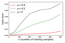
Theorem 18 implies that the stability bound decreases inversely with the size of the training set. It increases as the momentum parameter μ𝜇\mu increases. These properties are also verified in our experimental evaluation.666Our purpose in this work is not to show the superiority of SGDM or SGDEM, in terms of the stability bound, over SGD. Given the known advantage of SGDM in terms of speeding up training, our purpose is to further analyze the stability/generalization properties of SGDM and SGDEM.

The theoretically advocated momentum parameters in (Polyak, 1964; Nesterov, 1983) are based on convergence analysis of gradient descent with momentum, and do not account for generalization. Depending on the condition number of the problem, these values may not satisfy the range of momentum in Theorem 18. These values are not necessarily optimal for P-SGDM, in terms of our objective of true risk. Our goal in Theorem 18 is to show nontrivial cases that P-SGDM satisfies uniform stability.

Remark 19

Compared with the stability bound in (Hardt et al., 2016) for SGD, both bounds are in O(1/n)𝑂1𝑛O(1/n). Our bound in Theorem 18 holds for α2β+γ𝛼2𝛽𝛾\alpha\leq\frac{2}{\beta+\gamma}, which is slightly less restrictive than the range of step-size in (Hardt et al., 2016, Theorem 3.9). By substituting μ=0𝜇0\mu=0 in Eq. 4.1, we note that the constant term of our bound, β+γβγ𝛽𝛾𝛽𝛾\frac{\beta+\gamma}{\beta\gamma}, is slightly larger than that of (Hardt et al., 2016, Theorem 3.9), which is 1/γ1𝛾{1}/{\gamma}. Compared with (Chen et al., ), our bound is independent of T𝑇T and our work analyzes the case of strongly convex loss.

Classical generalization bounds using Rademacher complexity, which measures the rate of uniform convergence, are obtained for linear predictors with various norm constraints (Shalev-Shwartz and Ben-David, 2014). Those classical generalization bounds are typically 𝒪(1/n)𝒪1𝑛{\cal O}(1/\sqrt{n}). For linear predictors with a Lipschitz loss and a strongly convex regularizer, by bounding Rademacher complexity, it has been shown that with high probability, the generalization error is bounded by 𝒪(1/n)𝒪1𝑛{\cal O}(1/\sqrt{n}) for all parameters in a certain bounded set (Kakade et al., 2008). The fast rates by Sridharan et al. (2008) for regularized linear prediction are built based on the notion of localized Rademacher complexity (Bartlett et al., 2002), which requires an additional boundedness on the dual norm of data mapping. Our high-probability generalization bound for general smooth Lipschitz loss functions in Appendix G is 𝒪(1/n)𝒪1𝑛{\cal O}(1/n).

Our stability analysis captures how the learning algorithm explores the hypothesis class, in particular, how the generalization gap depends on the momentum. More broadly, unlike stability, uniform convergence is not necessary for learning (based on the learnability definition in (Shalev-Shwartz et al., 2010)) in the general learning setting (Shalev-Shwartz et al., 2010).

Finally, in the case of strongly convex loss, we can further consider the minimization of the true risk as defined in Eq. 2.1, since we are able to derive an upper bound on the optimization error (shown in Appendix I). In Appendix J, we study how the uniform stability results in an upper bound on the true risk of P-SGDM. We first show that stability results similar to Theorem 18 hold even if the average parameter 𝐰^Tsubscript^𝐰𝑇\hat{\bf w}_{T} is considered as the output of algorithm A𝐴A. We then decompose the expected true risk into a stability error term and an optimization one. We also compare the final results with SGD with no momentum, and we show that one can achieve tighter bounds by using P-SGDM than vanilla SGD.

5 Experimental Evaluation

5.1 Nonconvex Loss
Refer to caption
Refer to caption
Refer to caption
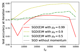
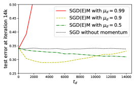
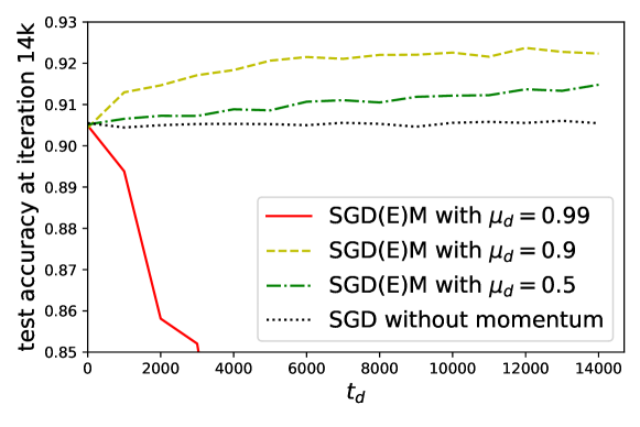
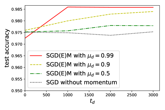
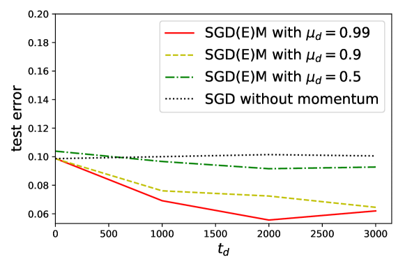
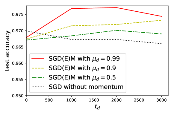
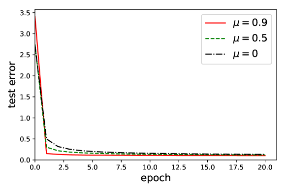
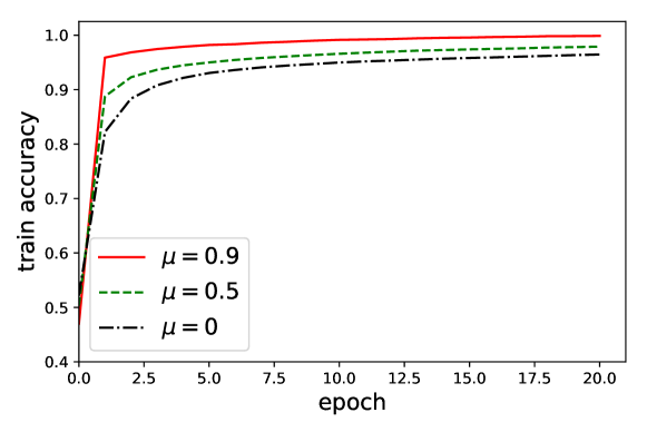
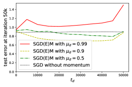
Figure 2: Test error (left) and test accuracy (middle) of ResNet-20 on CIFAR10. Test error of a feedforward fully connected neural network for notMNIST dataset (right).

In this section, we validate the insights obtained in our theoretical results using experimental evaluation. Our main goal is to study how adding momentum affects the generalization and convergence of SGD.

We first investigate the performance of SGDEM when applied to both CIFAR10 (Krizhevsky, ) and notMINIST datasets for nonconvex loss functions. We set T𝑇T to 50000 and 14000 for CIFAR10 and notMNIST experiments, respectively. For each value of μdsubscript𝜇𝑑\mu_{d}, we add momentum for 0-10 epochs. For each pair of (μd,td)subscript𝜇𝑑subscript𝑡𝑑(\mu_{d},t_{d}), we repeat the experiments 10 times with random initializations. SGDM can be viewed as a special form of SGDEM when the momentum is added for the entire training (i.e., td=Tsubscript𝑡𝑑𝑇t_{d}=T). For 10 epochs and without data augmentation, we train ResNet-20 on CIFAR10 and a feedforward fully connected neural network with 1000 hidden nodes on notMINIST. For the feedforward fully connected neural network, we use ReLU activation functions, a cross-entropy loss function, and a softmax output layer with Xavier initialization to initialize the weights (Glorot and Bengio, 2010).777We observe similar results for smooth activation functions. We set the step-size α=0.01𝛼0.01\alpha=0.01. The minibatch size is set to 10. We use 10 (SGDEM) realizations to evaluate the average performance. We compare the test performance of SGD without momentum with that of SGDEM under μd=0.5subscript𝜇𝑑0.5\mu_{d}=0.5, μd=0.9subscript𝜇𝑑0.9\mu_{d}=0.9, and μd=0.99subscript𝜇𝑑0.99\mu_{d}=0.99.

Outperforming both SGD and SGDM. We show the test error and test accuracy versus tdsubscript𝑡𝑑t_{d} under SGDEM for CIFAR10 dataset in Fig. 2 (left and middle). We observe that adding momentum for the entire training (i.e., td=Tsubscript𝑡𝑑𝑇t_{d}=T or SGDM) is useful when the momentum parameter is small. For different μdsubscript𝜇𝑑\mu_{d} values, we notice there exists an optimal tdsubscript𝑡𝑑t_{d} in Fig. 2 (left) when test error is minimized. We plot the test error versus tdsubscript𝑡𝑑t_{d} for notMNIST dataset in Fig. 2 (right). The test accuracy is shown in Appendix L. We observe an overshooting phenomenon for μd=0.99subscript𝜇𝑑0.99\mu_{d}=0.99, which is consistent with our convergence analysis in Theorem 25. We observe similar phenomenon when we train a feedforward fully connected neural network with 1000 hidden nodes on MINIST dataset. In terms of test accuracy, we observe that it is not helpful to use a momentum parameter, μd1subscript𝜇𝑑1\mu_{d}\approx 1, for the entire training. In an online framework with high dimensional parameters, early momentum is particularly useful since we can minimize memory utilization as SGDEM does not require 𝐰t1subscript𝐰𝑡1{\bf w}_{t-1} for the entire iterative updates.

Table 1: Ablation studies where we optimize performance of SGD and SGDM by obtaining the minimum test error over step-sizes α{0.1,0.01,0.001,0.0001}𝛼0.10.010.0010.0001\alpha\in\{0.1,0.01,0.001,0.0001\} and momentum parameters μ{0,0.5,0.9,0.99}𝜇00.50.90.99\mu\in\{0,0.5,0.9,0.99\}. We do not tune tdsubscript𝑡𝑑t_{d} and used the fixed td=3000subscript𝑡𝑑3000t_{d}=3000. The rest of the setup is similar to Fig. 2 (right).
SGD SGDEM SGDM
Test error 0.3596 ±plus-or-minus\pm 0.0142 0.2892 ±plus-or-minus\pm 0.0042 0.3194 ±plus-or-minus\pm 0.0030

To see whether SGDM is able to match performance of SGDEM by further tuning hyperparameters, in Table 1, we show the results of an ablation study where we minimize the test error of SGD and SGDM by optimizing over step-sizes α{0.1,0.01,0.001,0.0001}𝛼0.10.010.0010.0001\alpha\in\{0.1,0.01,0.001,0.0001\} and momentum parameters μ{0,0.5,0.9,0.99}𝜇00.50.90.99\mu\in\{0,0.5,0.9,0.99\}. For SGDEM, we do not tune tdsubscript𝑡𝑑t_{d} and used the fixed td=3000subscript𝑡𝑑3000t_{d}=3000. The rest of the setup is similar to Fig. 2 (right). We repeat the experiments for 5 times to report confidence intervals. These results show that even under tuned hyperparameters, SGDEM outperforms both SGDM and SGD in terms of test error.

Distributed training on ImageNet.

Fig. 1 shows validation loss and generalization error of SGDEM at epoch 90 when training ResNet-18 on ImageNet in a practical data-parallel setting with 4 GPUs under tuned step-sizes for SGD and SGDM. We observe that the minimum generalization error happens if the momentum is applied for 50 epochs. In Fig. 3, we plot validation accuracy and generalization gap of SGDEM at epoch 90. Similar to the loss results, we observe that the minimum generalization error happens if the momentum is applied for 50 epochs. Our accuracy results are on par with existing results (He et al., 2016).
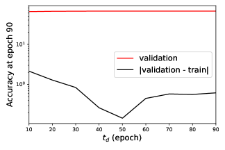
Refer to caption
Figure 3: Validation accuracy and generalization gap of SGDEM when training ResNet-18 on ImageNet in a distributed setting with 4 GPUs under tuned step-size and global minibatch size of 128. For each tdsubscript𝑡𝑑t_{d}, the momentum is set to μd=0.9subscript𝜇𝑑0.9\mu_{d}=0.9 in the first tdsubscript𝑡𝑑t_{d} epochs and then zero for the next 90td90subscript𝑡𝑑90-t_{d} epochs. SGDM is a special form of SGDEM with td=90subscript𝑡𝑑90t_{d}=90.

Details of ImageNet experiments.

The global minibatch size and weight decay are set to 128 and 5×1055superscript1055\times 10^{-5}, respectively. For each tdsubscript𝑡𝑑t_{d}, the momentum is set to μd=0.9subscript𝜇𝑑0.9\mu_{d}=0.9 in the first tdsubscript𝑡𝑑t_{d} epochs and then zero for the next 90td90subscript𝑡𝑑90-t_{d} epochs. We use a cluster with 4 NVIDIA 2080 Ti GPUs with the following CPU details: Intel(R) Xeon(R) CPU E5-2650 v4 @ 2.20GHz; 48 cores; GPU2GPU bandwidth: unidirectional 10GB/s and bidirectional 15GB/s.

5.2 Strongly Convex Loss
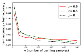
Refer to caption
Refer to caption
Refer to caption
Figure 4: Generalization error (left) and training error (middle) of logistic regression (cross entropy loss) for notMNIST dataset with T=1000𝑇1000T=1000 iterations . Test accuracy of logistic regression for notMNIST dataset with n=500𝑛500n=500 (right).

We now study the performance of SGDEM for a smooth and strongly convex loss function. We train a logistic regression model with the weight decay regularization on notMNIST and MNIST. The setup’s details are provided in Appendix L. We plot the test error and test accuracy versus tdsubscript𝑡𝑑t_{d} under SGDEM for notMNIST and MNIST in Appendix L and observe that, unlike the case of nonconvex loss functions, it does not hurt to add momentum for the entire training. We then focus on SGDM and compare the optimization and generalization performance of vanilla SGD with that of SGDM under μ=0.5𝜇0.5\mu=0.5 and μ=0.9𝜇0.9\mu=0.9, which are common momentum values used in practice (Goodfellow et al., 2016, Section 8.3.2).

Hurting generalization error and improving training error.

In Fig. 4 (left) and (middle), we plot generalization and training error versus n𝑛n with fixed T𝑇T and observe that generalization error decreases as n𝑛n increases for all values of μ𝜇\mu, which is suggested by our stability upper bound in Theorem 18. In addition, for sufficiently large n𝑛n, we observe that the generalization error increases with μ𝜇\mu, consistent with Theorem 18. On the other hand, training error increases as n𝑛n increases with fixed T𝑇T, which is expected. We can observe that adding momentum reduces training error as it improves the convergence rate.

Negligible improvement of test accuracy.

In Fig. 4 (right), we plot test accuracy versus T𝑇T with fixed n𝑛n (See Appendix L for training error, training accuracy, and test error). As the number of epochs increases, we note that the benefit of momentum on the test accuracy becomes negligible. This happens because adding momentum results in a higher generalization error thus penalizing the gain in training error.

6 Conclusions and Future Work

We study the generalization error of SGDEM under mild technical conditions. We show that there exists a convex loss function for which the stability gap for multiple epochs of SGDM becomes unbounded and investigate a modified momentum-based update rule, i.e., SGDEM. We establish a bound on the generalization error of SGDEM for the class of smooth Lipschitz loss functions. Our results confirm that deep neural networks can be trained for multiple epochs of SGDEM while their generalization errors are bounded. We also study the convergence of SGDEM in terms of a bound on the expected norm of the gradient. Then, for the case of strongly convex loss functions, we establish an upper bound on the generalization error, which decreases with the size of the training set, and increases as the momentum parameter is increased. We establish an upper bound on the expected difference between the true risk of P-SGDM and the global minimum of the empirical risk. Finally, we present experimental evaluation and show that the numerical results are consistent with our theoretical bounds and SGDEM is an effective algorithm for nonconvex problems.

Beyond uniform stability analysis, which is sufficient for generalization, developing necessary conditions for generalization of various learning algorithms remains an open problem. In particular, “on-average” stability is a more relaxed notion and depends on the data-generating distribution (Shalev-Shwartz et al., 2010). Finally, practical methods for adaptive training, such as Adam, use a variation of the heavy-ball momentum (Kingma and Ba, 2015). Adapting our analysis for such extensions is also an interesting area of future work.


Acknowledgments and Disclosure of Funding

This work was supported by 1) the Research Council of Norway through its Centres of Excellence scheme, Integreat - Norwegian Centre for knowledge-driven machine learning, project number 332645; 2) the Research Council of Norway through its Centre for Research-based Innovation funding scheme (Visual Intelligence under grant no. 309439), and Consortium Partners; 3) Hasler Foundation Program: Hasler Responsible AI (project number 21043); 4) the Swiss National Science Foundation (SNSF) under grant number 200021_205011; 5) the Natural Sciences and Engineering Research Council of Canada under a Discovery Grant.

Content of the appendix.

The appendix is organized as follows:

  • In Appendix A, we show that the stability gap for multiple epochs of SGDM may become unbounded for any step-size schedule.

  • Theorem 8 (convergence of SGDEM) is proved in Appendix B.

  • Convergence of SGDEM with constant step-size is provided in Appendix C.

  • Convergence guarantees for SGDEM with other time-dependent step-sizes are provided in  Appendix D.

  • A sufficient condition for the upper bound in Theorem 25 to become monotonically decreasing is provided in Appendix E.

  • Benefit of using momentum in terms of convergence is elaborated in  Appendix F.

  • High-probability generalization bounds for SGDEM are established in Appendix G.

  • Theorem 18 (stability of strongly convex problems) is proved in  Appendix H.

  • Convergence bound for strongly convex loss is provided in Appendix I.

  • An upper bound on true risk of strongly convex loss is established in Appendix J.

  • Generalization error of SGDEM with αt=α0/tsubscript𝛼𝑡subscript𝛼0𝑡\alpha_{t}=\alpha_{0}/\sqrt{t} is discussed in Appendix K.

  • Additional experimental details are included in Appendix L.

In our analysis of the stability of SGDM, we will consider the following two properties of the growth of the update rule. Let ΩΩ\Omega denote the model parameter space. Consider a general update rule G𝐺G which maps 𝐰Ω𝐰Ω{\bf w}\in\Omega to another point G(𝐰)Ω𝐺𝐰ΩG({\bf w})\in\Omega. Our goal is to track the divergence of two different iterative sequences of update rules with the same starting point.

Definition 20

An update rule G𝐺G is η𝜂\eta-expansive if

sup𝐯,𝐰ΩG(𝐯)G(𝐰)𝐯𝐰η.subscriptsupremum𝐯𝐰Ωnorm𝐺𝐯𝐺𝐰norm𝐯𝐰𝜂\displaystyle\sup_{{\bf v},{\bf w}\in\Omega}\frac{\|G({\bf v})-G({\bf w})\|}{\|{\bf v}-{\bf w}\|}\leq\eta.
Definition 21

An update rule G𝐺G is σ𝜎\sigma-bounded if

sup𝐰Ω𝐰G(𝐰)σ.subscriptsupremum𝐰Ωnorm𝐰𝐺𝐰𝜎\displaystyle\sup_{{\bf w}\in\Omega}\|{\bf w}-G({\bf w})\|\leq\sigma.

Appendix A Importance of early momentum on bounding the stability gap

To highlight the importance of early momentum on bounding the stability gap, in this section, we show that the stability gap for multiple epochs of SGDM may become unbounded for any step-size schedule. This includes α1=1subscript𝛼11\alpha_{1}=1 and αj=0subscript𝛼𝑗0\alpha_{j}=0 for j>1𝑗1j>1, i.e., the gradient term is added only in the first iteration. We also establish a Ω(Tn)Ω𝑇𝑛\Omega(\frac{T}{n}) lower bound for SGDM on Example 1 even with a time-decaying step-size, which shows that it is important to control both step-size and momentum to establish uniform stability.

Theorem 22

For Example 1 with datasets described in Theorem 3 and for any step-size schedule, there exists a momentum such that the stability gap for SGDM is lower bounded by Ω(Tn)Ω𝑇𝑛\Omega(\frac{T}{n}).

In addition, if αjαminsubscript𝛼𝑗subscript𝛼\alpha_{j}\geq\alpha_{\min} for j=1,2,,ηT𝑗12𝜂𝑇j=1,2,\ldots,\eta T where αminsubscript𝛼\alpha_{\min} and η<1𝜂1\eta<1 are some constants that do not depend on T𝑇T, then the stability gap for SGDM is lower bounded by Ω(Tn)Ω𝑇𝑛\Omega(\frac{T}{n}) for any momentum μ>0𝜇0\mu>0.

Proof Following the proofs of Theorem 3 for SGDM with α1>0subscript𝛼10\alpha_{1}>0, we have

𝔼A[|(𝗐T;𝐳)(𝗐T;𝐳)|]2α1L2nj=0T1μj.subscript𝔼𝐴delimited-[]subscript𝗐𝑇𝐳subscriptsuperscript𝗐𝑇𝐳2subscript𝛼1superscript𝐿2𝑛superscriptsubscript𝑗0𝑇1superscript𝜇𝑗\displaystyle\mathbb{E}_{A}[|\ell({\mathsf{w}}_{T};{\bf z})-\ell({\mathsf{w}}^{\prime}_{T};{\bf z})|]\geq\frac{2\alpha_{1}L^{2}}{n}\sum_{j=0}^{T-1}\mu^{j}.

Substituting μ=1𝜇1\mu=1, 𝔼A[|(𝗐T;𝐳)(𝗐T;𝐳)|]subscript𝔼𝐴delimited-[]subscript𝗐𝑇𝐳subscriptsuperscript𝗐𝑇𝐳\mathbb{E}_{A}[|\ell({\mathsf{w}}_{T};{\bf z})-\ell({\mathsf{w}}^{\prime}_{T};{\bf z})|] is lower bounded by Ω(Tn)Ω𝑇𝑛\Omega(\frac{T}{n}).

For the second part of the theorem, suppose αjαminsubscript𝛼𝑗subscript𝛼\alpha_{j}\geq\alpha_{\min} for j=1,2,,ηT𝑗12𝜂𝑇j=1,2,\ldots,\eta T. Then we have

𝔼A[|(𝗐T;𝐳)(𝗐T;𝐳)|]2αminL2nj=0ηT1(Tj)μjsubscript𝔼𝐴delimited-[]subscript𝗐𝑇𝐳subscriptsuperscript𝗐𝑇𝐳2subscript𝛼superscript𝐿2𝑛superscriptsubscript𝑗0𝜂𝑇1𝑇𝑗superscript𝜇𝑗\displaystyle\mathbb{E}_{A}[|\ell({\mathsf{w}}_{T};{\bf z})-\ell({\mathsf{w}}^{\prime}_{T};{\bf z})|]\geq\frac{2\alpha_{\min}L^{2}}{n}\sum_{j=0}^{\eta T-1}(T-j)\mu^{j}

and 𝔼A[|(𝗐T;𝐳)(𝗐T;𝐳)|]subscript𝔼𝐴delimited-[]subscript𝗐𝑇𝐳subscriptsuperscript𝗐𝑇𝐳\mathbb{E}_{A}[|\ell({\mathsf{w}}_{T};{\bf z})-\ell({\mathsf{w}}^{\prime}_{T};{\bf z})|] is lower bounded by Ω(Tn)Ω𝑇𝑛\Omega(\frac{T}{n}).  

Corollary 23

For Example 1 with datasets described in Theorem 3 and for time-decaying step-size, the stability gap for SGDM is lower bounded by Ω(Tn)Ω𝑇𝑛\Omega(\frac{T}{n}) for any momentum μ>0𝜇0\mu>0.

Proof It follows immediately from the proof of Theorem 4.  

Appendix B Proof of Theorem 8 (convergence of SGDEM)

The following lemmas are useful for our proofs:

Lemma 24

For any integers t𝑡t, p𝑝p, and q𝑞q, such that 0tT10𝑡𝑇10\leq t\leq T-1, p<T𝑝𝑇p<T, and q<Tt𝑞𝑇𝑡q<T-t, and for any sequences a0,a1,subscript𝑎0subscript𝑎1a_{0},a_{1},\ldots, and b0,b1,subscript𝑏0subscript𝑏1b_{0},b_{1},\ldots, we have

i=pTaij=qitbj=i=qTtbij=i+tTaj.superscriptsubscript𝑖𝑝𝑇subscript𝑎𝑖superscriptsubscript𝑗𝑞𝑖𝑡subscript𝑏𝑗superscriptsubscript𝑖𝑞𝑇𝑡subscript𝑏𝑖superscriptsubscript𝑗𝑖𝑡𝑇subscript𝑎𝑗\displaystyle\sum_{i=p}^{T}a_{i}\sum_{j=q}^{i-t}b_{j}=\sum_{i=q}^{T-t}b_{i}\sum_{j=i+t}^{T}a_{j}.

Proof We prove by induction. It clearly holds for T=1𝑇1T=1. Suppose it holds for all k<T𝑘𝑇k<T. Then, we have

i=pk+1aij=qitbj=i=pkaij=qitbj+ak+1j=qk+1tbj=i=qktbij=i+tkaj+ak+1j=qk+1tbj=i=qktbij=i+tkaj+ak+1j=qktbj+ak+1bk+1t=i=qktbij=i+tk+1aj+ak+1bk+1t=i=qk+1tbij=i+tk+1aj.superscriptsubscript𝑖𝑝𝑘1subscript𝑎𝑖superscriptsubscript𝑗𝑞𝑖𝑡subscript𝑏𝑗superscriptsubscript𝑖𝑝𝑘subscript𝑎𝑖superscriptsubscript𝑗𝑞𝑖𝑡subscript𝑏𝑗subscript𝑎𝑘1superscriptsubscript𝑗𝑞𝑘1𝑡subscript𝑏𝑗superscriptsubscript𝑖𝑞𝑘𝑡subscript𝑏𝑖superscriptsubscript𝑗𝑖𝑡𝑘subscript𝑎𝑗subscript𝑎𝑘1superscriptsubscript𝑗𝑞𝑘1𝑡subscript𝑏𝑗superscriptsubscript𝑖𝑞𝑘𝑡subscript𝑏𝑖superscriptsubscript𝑗𝑖𝑡𝑘subscript𝑎𝑗subscript𝑎𝑘1superscriptsubscript𝑗𝑞𝑘𝑡subscript𝑏𝑗subscript𝑎𝑘1subscript𝑏𝑘1𝑡superscriptsubscript𝑖𝑞𝑘𝑡subscript𝑏𝑖superscriptsubscript𝑗𝑖𝑡𝑘1subscript𝑎𝑗subscript𝑎𝑘1subscript𝑏𝑘1𝑡superscriptsubscript𝑖𝑞𝑘1𝑡subscript𝑏𝑖superscriptsubscript𝑗𝑖𝑡𝑘1subscript𝑎𝑗\displaystyle\begin{split}\sum_{i=p}^{k+1}a_{i}\sum_{j=q}^{i-t}b_{j}&=\sum_{i=p}^{k}a_{i}\sum_{j=q}^{i-t}b_{j}+a_{k+1}\sum_{j=q}^{k+1-t}b_{j}\\ &=\sum_{i=q}^{k-t}b_{i}\sum_{j=i+t}^{k}a_{j}+a_{k+1}\sum_{j=q}^{k+1-t}b_{j}\\ &=\sum_{i=q}^{k-t}b_{i}\sum_{j=i+t}^{k}a_{j}+a_{k+1}\sum_{j=q}^{k-t}b_{j}+a_{k+1}b_{k+1-t}\\ &=\sum_{i=q}^{k-t}b_{i}\sum_{j=i+t}^{k+1}a_{j}+a_{k+1}b_{k+1-t}\\ &=\sum_{i=q}^{k+1-t}b_{i}\sum_{j=i+t}^{k+1}a_{j}.\end{split} (B.1)


As two special cases of  Lemma 24, we obtain (Li and Orabona, 2020, Lemma 4) by substituting q=1,t=0,p=1formulae-sequence𝑞1formulae-sequence𝑡0𝑝1q=1,\leavevmode\nobreak\ t=0,\leavevmode\nobreak\ p=1 and q=0,t=1,p=1formulae-sequence𝑞0formulae-sequence𝑡1𝑝1q=0,\leavevmode\nobreak\ t=1,\leavevmode\nobreak\ p=1:

i=1Taij=1ibjsuperscriptsubscript𝑖1𝑇subscript𝑎𝑖superscriptsubscript𝑗1𝑖subscript𝑏𝑗\displaystyle\sum_{i=1}^{T}a_{i}\sum_{j=1}^{i}b_{j} =i=1Tbij=iTaj,absentsuperscriptsubscript𝑖1𝑇subscript𝑏𝑖superscriptsubscript𝑗𝑖𝑇subscript𝑎𝑗\displaystyle=\sum_{i=1}^{T}b_{i}\sum_{j=i}^{T}a_{j},
i=1Taij=0i1bjsuperscriptsubscript𝑖1𝑇subscript𝑎𝑖superscriptsubscript𝑗0𝑖1subscript𝑏𝑗\displaystyle\sum_{i=1}^{T}a_{i}\sum_{j=0}^{i-1}b_{j} =i=1T1bij=i+1Taj.absentsuperscriptsubscript𝑖1𝑇1subscript𝑏𝑖superscriptsubscript𝑗𝑖1𝑇subscript𝑎𝑗\displaystyle=\sum_{i=1}^{T-1}b_{i}\sum_{j=i+1}^{T}a_{j}.

To facilitate the convergence analysis, we define 𝗾t:=𝘄t𝘄t1assignsubscript𝗾𝑡subscript𝘄𝑡subscript𝘄𝑡1{\bm{\mathsf{q}}}_{t}:={\bm{\mathsf{w}}}_{t}-{\bm{\mathsf{w}}}_{t-1} with 𝗾0=0subscript𝗾00{\bm{\mathsf{q}}}_{0}=0 and 𝗾1=0subscript𝗾10{\bm{\mathsf{q}}}_{1}=0. It is not difficult to show that 𝗾t+1=μd𝗾tαt𝐰(𝘄t;𝐳𝗂t)subscript𝗾𝑡1subscript𝜇𝑑subscript𝗾𝑡subscript𝛼𝑡subscript𝐰subscript𝘄𝑡subscript𝐳subscript𝗂𝑡{\bm{\mathsf{q}}}_{t+1}=\mu_{d}{\bm{\mathsf{q}}}_{t}-\alpha_{t}\nabla_{\bf w}\ell({\bm{\mathsf{w}}}_{t};{\bf z}_{{\mathsf{i}}_{t}}). Since the empirical risk R𝒮subscript𝑅𝒮R_{\cal S} is a β𝛽\beta-smooth function, we have

R𝒮(𝘄t+1)R𝒮(𝘄t)+R𝒮(𝘄t)𝗾t+1+β2𝗾t+12.subscript𝑅𝒮subscript𝘄𝑡1subscript𝑅𝒮subscript𝘄𝑡subscript𝑅𝒮superscriptsubscript𝘄𝑡topsubscript𝗾𝑡1𝛽2superscriptdelimited-∥∥subscript𝗾𝑡12\displaystyle\begin{split}R_{\cal S}({\bm{\mathsf{w}}}_{t+1})&\leq R_{\cal S}({\bm{\mathsf{w}}}_{t})+\nabla R_{\cal S}({\bm{\mathsf{w}}}_{t})^{\top}{\bm{\mathsf{q}}}_{t+1}+\frac{\beta}{2}\|{\bm{\mathsf{q}}}_{t+1}\|^{2}.\end{split} (B.2)

Based on the definition of 𝗾tsubscript𝗾𝑡{\bm{\mathsf{q}}}_{t}, the inner-product term in Eq. B.2 is bounded:

R𝒮(𝘄t)𝗾t+1=μdR𝒮(𝘄t)𝗾tαtR𝒮(𝘄t)(𝘄t;𝐳𝗂t)=μdR𝒮(𝘄t1)𝗾t+μd(R𝒮(𝘄t)R𝒮(𝘄t1))𝗾tαtR𝒮(𝘄t)(𝘄t;𝐳𝗂t)μdR𝒮(𝘄t1)𝗾t+μdR𝒮(𝘄t)R𝒮(𝘄t1)𝗾tαtR𝒮(𝘄t)(𝘄t;𝐳𝗂t)μdR𝒮(𝘄t1)𝗾t+μdβ𝗾t2αtR𝒮(𝘄t)(𝘄t;𝐳𝗂t)subscript𝑅𝒮superscriptsubscript𝘄𝑡topsubscript𝗾𝑡1subscript𝜇𝑑subscript𝑅𝒮superscriptsubscript𝘄𝑡topsubscript𝗾𝑡subscript𝛼𝑡subscript𝑅𝒮superscriptsubscript𝘄𝑡topsubscript𝘄𝑡subscript𝐳subscript𝗂𝑡subscript𝜇𝑑subscript𝑅𝒮superscriptsubscript𝘄𝑡1topsubscript𝗾𝑡subscript𝜇𝑑superscriptsubscript𝑅𝒮subscript𝘄𝑡subscript𝑅𝒮subscript𝘄𝑡1topsubscript𝗾𝑡subscript𝛼𝑡subscript𝑅𝒮superscriptsubscript𝘄𝑡topsubscript𝘄𝑡subscript𝐳subscript𝗂𝑡subscript𝜇𝑑subscript𝑅𝒮superscriptsubscript𝘄𝑡1topsubscript𝗾𝑡subscript𝜇𝑑delimited-∥∥subscript𝑅𝒮subscript𝘄𝑡subscript𝑅𝒮subscript𝘄𝑡1delimited-∥∥subscript𝗾𝑡subscript𝛼𝑡subscript𝑅𝒮superscriptsubscript𝘄𝑡topsubscript𝘄𝑡subscript𝐳subscript𝗂𝑡subscript𝜇𝑑subscript𝑅𝒮superscriptsubscript𝘄𝑡1topsubscript𝗾𝑡subscript𝜇𝑑𝛽superscriptdelimited-∥∥subscript𝗾𝑡2subscript𝛼𝑡subscript𝑅𝒮superscriptsubscript𝘄𝑡topsubscript𝘄𝑡subscript𝐳subscript𝗂𝑡\displaystyle\begin{split}\nabla R_{\cal S}({\bm{\mathsf{w}}}_{t})^{\top}{\bm{\mathsf{q}}}_{t+1}&=\mu_{d}\nabla R_{\cal S}({\bm{\mathsf{w}}}_{t})^{\top}{\bm{\mathsf{q}}}_{t}-\alpha_{t}\nabla R_{\cal S}({\bm{\mathsf{w}}}_{t})^{\top}\nabla\ell({\bm{\mathsf{w}}}_{t};{\bf z}_{{\mathsf{i}}_{t}})\\ &=\mu_{d}\nabla R_{\cal S}({\bm{\mathsf{w}}}_{t-1})^{\top}{\bm{\mathsf{q}}}_{t}+\mu_{d}\big{(}\nabla R_{\cal S}({\bm{\mathsf{w}}}_{t})-\nabla R_{\cal S}({\bm{\mathsf{w}}}_{t-1})\big{)}^{\top}{\bm{\mathsf{q}}}_{t}\\ &\quad-\alpha_{t}\nabla R_{\cal S}({\bm{\mathsf{w}}}_{t})^{\top}\nabla\ell({\bm{\mathsf{w}}}_{t};{\bf z}_{{\mathsf{i}}_{t}})\\ &\leq\mu_{d}\nabla R_{\cal S}({\bm{\mathsf{w}}}_{t-1})^{\top}{\bm{\mathsf{q}}}_{t}+\mu_{d}\|\nabla R_{\cal S}({\bm{\mathsf{w}}}_{t})-\nabla R_{\cal S}({\bm{\mathsf{w}}}_{t-1})\|\|{\bm{\mathsf{q}}}_{t}\|\\ &\quad-\alpha_{t}\nabla R_{\cal S}({\bm{\mathsf{w}}}_{t})^{\top}\nabla\ell({\bm{\mathsf{w}}}_{t};{\bf z}_{{\mathsf{i}}_{t}})\\ &\leq\mu_{d}\nabla R_{\cal S}({\bm{\mathsf{w}}}_{t-1})^{\top}{\bm{\mathsf{q}}}_{t}+\mu_{d}\beta\|{\bm{\mathsf{q}}}_{t}\|^{2}-\alpha_{t}\nabla R_{\cal S}({\bm{\mathsf{w}}}_{t})^{\top}\nabla\ell({\bm{\mathsf{w}}}_{t};{\bf z}_{{\mathsf{i}}_{t}})\end{split} (B.3)

where the last inequality holds due to smoothness. Unraveling the recursion Eq. B.3, we have

R𝒮(𝘄t)𝗾t+1subscript𝑅𝒮superscriptsubscript𝘄𝑡topsubscript𝗾𝑡1\displaystyle\nabla R_{\cal S}({\bm{\mathsf{w}}}_{t})^{\top}{\bm{\mathsf{q}}}_{t+1} βi=0t1μdti𝗾i+12i=1tμdtiαiR𝒮(𝘄i)(𝘄i;𝐳𝗂i)absent𝛽superscriptsubscript𝑖0𝑡1superscriptsubscript𝜇𝑑𝑡𝑖superscriptnormsubscript𝗾𝑖12superscriptsubscript𝑖1𝑡superscriptsubscript𝜇𝑑𝑡𝑖subscript𝛼𝑖subscript𝑅𝒮superscriptsubscript𝘄𝑖topsubscript𝘄𝑖subscript𝐳subscript𝗂𝑖\displaystyle\leq\beta\sum_{i=0}^{t-1}\mu_{d}^{t-i}\|{\bm{\mathsf{q}}}_{i+1}\|^{2}-\sum_{i=1}^{t}\mu_{d}^{t-i}\alpha_{i}\nabla R_{\cal S}({\bm{\mathsf{w}}}_{i})^{\top}\nabla\ell({\bm{\mathsf{w}}}_{i};{\bf z}_{{\mathsf{i}}_{i}})

For simplicity of analysis, we first suppose that the momentum is applied in T𝑇T steps. Then we modify the bound considering it is set to zero after tdsubscript𝑡𝑑t_{d} steps. Substituting this bound in Eq. B.2 and summing for t=1,,T𝑡1𝑇t=1,\ldots,T, we have

R𝒮(𝘄T+1)R𝒮(𝘄0)+βt=1Ti=1t1μdti𝗾i+12+β2t=1T𝗾t+12t=1Ti=1tμdtiαiR𝒮(𝘄i)(𝘄i;𝐳𝗂i).subscript𝑅𝒮subscript𝘄𝑇1subscript𝑅𝒮subscript𝘄0𝛽superscriptsubscript𝑡1𝑇superscriptsubscript𝑖1𝑡1superscriptsubscript𝜇𝑑𝑡𝑖superscriptdelimited-∥∥subscript𝗾𝑖12𝛽2superscriptsubscript𝑡1𝑇superscriptdelimited-∥∥subscript𝗾𝑡12superscriptsubscript𝑡1𝑇superscriptsubscript𝑖1𝑡superscriptsubscript𝜇𝑑𝑡𝑖subscript𝛼𝑖subscript𝑅𝒮superscriptsubscript𝘄𝑖topsubscript𝘄𝑖subscript𝐳subscript𝗂𝑖\displaystyle\begin{split}R_{\cal S}({\bm{\mathsf{w}}}_{T+1})&\leq R_{\cal S}({\bm{\mathsf{w}}}_{0})+\beta\sum_{t=1}^{T}\sum_{i=1}^{t-1}\mu_{d}^{t-i}\|{\bm{\mathsf{q}}}_{i+1}\|^{2}+\frac{\beta}{2}\sum_{t=1}^{T}\|{\bm{\mathsf{q}}}_{t+1}\|^{2}\\ &\quad-\sum_{t=1}^{T}\sum_{i=1}^{t}\mu_{d}^{t-i}\alpha_{i}\nabla R_{\cal S}({\bm{\mathsf{w}}}_{i})^{\top}\nabla\ell({\bm{\mathsf{w}}}_{i};{\bf z}_{{\mathsf{i}}_{i}}).\end{split} (B.4)

Using Lemma 24, we expand the the second and fourth terms in the upper bound Eq. B.4:

βt=1Ti=1t1μdti𝗾i+12=βt=1T1𝗾t+12μdti=t+1Tμdi=βt=1T1μdμdTt+11μd𝗾t+12βμd1μdt=1T1𝗾t+12.𝛽superscriptsubscript𝑡1𝑇superscriptsubscript𝑖1𝑡1superscriptsubscript𝜇𝑑𝑡𝑖superscriptdelimited-∥∥subscript𝗾𝑖12𝛽superscriptsubscript𝑡1𝑇1superscriptdelimited-∥∥subscript𝗾𝑡12superscriptsubscript𝜇𝑑𝑡superscriptsubscript𝑖𝑡1𝑇superscriptsubscript𝜇𝑑𝑖𝛽superscriptsubscript𝑡1𝑇1subscript𝜇𝑑superscriptsubscript𝜇𝑑𝑇𝑡11subscript𝜇𝑑superscriptdelimited-∥∥subscript𝗾𝑡12𝛽subscript𝜇𝑑1subscript𝜇𝑑superscriptsubscript𝑡1𝑇1superscriptdelimited-∥∥subscript𝗾𝑡12\displaystyle\begin{split}\beta\sum_{t=1}^{T}\sum_{i=1}^{t-1}\mu_{d}^{t-i}\|{\bm{\mathsf{q}}}_{i+1}\|^{2}&=\beta\sum_{t=1}^{T-1}\|{\bm{\mathsf{q}}}_{t+1}\|^{2}\mu_{d}^{-t}\sum_{i=t+1}^{T}\mu_{d}^{i}\\ &=\beta\sum_{t=1}^{T-1}\frac{\mu_{d}-\mu_{d}^{T-t+1}}{1-\mu_{d}}\|{\bm{\mathsf{q}}}_{t+1}\|^{2}\\ &\leq\frac{\beta\mu_{d}}{1-\mu_{d}}\sum_{t=1}^{T-1}\|{\bm{\mathsf{q}}}_{t+1}\|^{2}.\end{split} (B.5)

Furthermore, we have

t=1Ti=1tμdtiαiR𝒮(𝘄i)(𝘄i;𝐳𝗂i)=t=1Ti=1tμdtiαiR𝒮(𝘄i)R𝒮(𝘄i)+t=1Ti=1tμdtiαiR𝒮(𝘄i)(R𝒮(𝘄i)(𝘄i;𝐳𝗂i))=t=1TμdtαtR𝒮(𝘄t)2i=tTμdi+t=1TμdtαtR𝒮(𝘄t)(R𝒮(𝘄t)(𝘄t;𝐳𝗂t))i=tTμdi=t=1T1μdTt+11μdαtR𝒮(𝘄t)2+t=1T1μdTt+11μdαtR𝒮(𝘄t)(R𝒮(𝘄t)(𝘄t;𝐳𝗂t))superscriptsubscript𝑡1𝑇superscriptsubscript𝑖1𝑡superscriptsubscript𝜇𝑑𝑡𝑖subscript𝛼𝑖subscript𝑅𝒮superscriptsubscript𝘄𝑖topsubscript𝘄𝑖subscript𝐳subscript𝗂𝑖superscriptsubscript𝑡1𝑇superscriptsubscript𝑖1𝑡superscriptsubscript𝜇𝑑𝑡𝑖subscript𝛼𝑖subscript𝑅𝒮superscriptsubscript𝘄𝑖topsubscript𝑅𝒮subscript𝘄𝑖superscriptsubscript𝑡1𝑇superscriptsubscript𝑖1𝑡superscriptsubscript𝜇𝑑𝑡𝑖subscript𝛼𝑖subscript𝑅𝒮superscriptsubscript𝘄𝑖topsubscript𝑅𝒮subscript𝘄𝑖subscript𝘄𝑖subscript𝐳subscript𝗂𝑖superscriptsubscript𝑡1𝑇superscriptsubscript𝜇𝑑𝑡subscript𝛼𝑡superscriptdelimited-∥∥subscript𝑅𝒮subscript𝘄𝑡2superscriptsubscript𝑖𝑡𝑇superscriptsubscript𝜇𝑑𝑖superscriptsubscript𝑡1𝑇superscriptsubscript𝜇𝑑𝑡subscript𝛼𝑡subscript𝑅𝒮superscriptsubscript𝘄𝑡topsubscript𝑅𝒮subscript𝘄𝑡subscript𝘄𝑡subscript𝐳subscript𝗂𝑡superscriptsubscript𝑖𝑡𝑇superscriptsubscript𝜇𝑑𝑖superscriptsubscript𝑡1𝑇1superscriptsubscript𝜇𝑑𝑇𝑡11subscript𝜇𝑑subscript𝛼𝑡superscriptdelimited-∥∥subscript𝑅𝒮subscript𝘄𝑡2superscriptsubscript𝑡1𝑇1superscriptsubscript𝜇𝑑𝑇𝑡11subscript𝜇𝑑subscript𝛼𝑡subscript𝑅𝒮superscriptsubscript𝘄𝑡topsubscript𝑅𝒮subscript𝘄𝑡subscript𝘄𝑡subscript𝐳subscript𝗂𝑡\displaystyle\begin{split}-\sum_{t=1}^{T}\sum_{i=1}^{t}\mu_{d}^{t-i}\alpha_{i}\nabla R_{\cal S}({\bm{\mathsf{w}}}_{i})^{\top}\nabla\ell({\bm{\mathsf{w}}}_{i};{\bf z}_{{\mathsf{i}}_{i}})&=-\sum_{t=1}^{T}\sum_{i=1}^{t}\mu_{d}^{t-i}\alpha_{i}\nabla R_{\cal S}({\bm{\mathsf{w}}}_{i})^{\top}\nabla R_{\cal S}({\bm{\mathsf{w}}}_{i})\\ &\quad+\sum_{t=1}^{T}\sum_{i=1}^{t}\mu_{d}^{t-i}\alpha_{i}\nabla R_{\cal S}({\bm{\mathsf{w}}}_{i})^{\top}\big{(}\nabla R_{\cal S}({\bm{\mathsf{w}}}_{i})-\nabla\ell({\bm{\mathsf{w}}}_{i};{\bf z}_{{\mathsf{i}}_{i}})\big{)}\\ &=-\sum_{t=1}^{T}\mu_{d}^{-t}\alpha_{t}\|\nabla R_{\cal S}({\bm{\mathsf{w}}}_{t})\|^{2}\sum_{i=t}^{T}\mu_{d}^{i}\\ &\quad+\sum_{t=1}^{T}\mu_{d}^{-t}\alpha_{t}\nabla R_{\cal S}({\bm{\mathsf{w}}}_{t})^{\top}\big{(}\nabla R_{\cal S}({\bm{\mathsf{w}}}_{t})-\nabla\ell({\bm{\mathsf{w}}}_{t};{\bf z}_{{\mathsf{i}}_{t}})\big{)}\sum_{i=t}^{T}\mu_{d}^{i}\\ &=-\sum_{t=1}^{T}\frac{1-\mu_{d}^{T-t+1}}{1-\mu_{d}}\alpha_{t}\|\nabla R_{\cal S}({\bm{\mathsf{w}}}_{t})\|^{2}\\ &\quad+\sum_{t=1}^{T}\frac{1-\mu_{d}^{T-t+1}}{1-\mu_{d}}\alpha_{t}\nabla R_{\cal S}({\bm{\mathsf{w}}}_{t})^{\top}\big{(}\nabla R_{\cal S}({\bm{\mathsf{w}}}_{t})-\nabla\ell({\bm{\mathsf{w}}}_{t};{\bf z}_{{\mathsf{i}}_{t}})\big{)}\end{split} (B.6)

Substituting Eqs. B.5 and B.6 into Eq. B.4 and rearranging the terms, we obtain

t=1T1μdTt+11μdαtR𝒮(𝘄t)2R𝒮(𝘄0)R𝒮(𝘄T+1)+β2t=1T𝗾t+12+t=1T1μdTt+11μdαtR𝒮(𝘄t)(R𝒮(𝘄t)(𝘄t;𝐳𝗂t))+βμd1μdt=1T1𝗾t+12.superscriptsubscript𝑡1𝑇1superscriptsubscript𝜇𝑑𝑇𝑡11subscript𝜇𝑑subscript𝛼𝑡superscriptdelimited-∥∥subscript𝑅𝒮subscript𝘄𝑡2subscript𝑅𝒮subscript𝘄0subscript𝑅𝒮subscript𝘄𝑇1𝛽2superscriptsubscript𝑡1𝑇superscriptdelimited-∥∥subscript𝗾𝑡12superscriptsubscript𝑡1𝑇1superscriptsubscript𝜇𝑑𝑇𝑡11subscript𝜇𝑑subscript𝛼𝑡subscript𝑅𝒮superscriptsubscript𝘄𝑡topsubscript𝑅𝒮subscript𝘄𝑡subscript𝘄𝑡subscript𝐳subscript𝗂𝑡𝛽subscript𝜇𝑑1subscript𝜇𝑑superscriptsubscript𝑡1𝑇1superscriptdelimited-∥∥subscript𝗾𝑡12\displaystyle\begin{split}\sum_{t=1}^{T}\frac{1-\mu_{d}^{T-t+1}}{1-\mu_{d}}\alpha_{t}\|\nabla R_{\cal S}({\bm{\mathsf{w}}}_{t})\|^{2}&\leq R_{\cal S}({\bm{\mathsf{w}}}_{0})-R_{\cal S}({\bm{\mathsf{w}}}_{T+1})+\frac{\beta}{2}\sum_{t=1}^{T}\|{\bm{\mathsf{q}}}_{t+1}\|^{2}\\ &\quad+\sum_{t=1}^{T}\frac{1-\mu_{d}^{T-t+1}}{1-\mu_{d}}\alpha_{t}\nabla R_{\cal S}({\bm{\mathsf{w}}}_{t})^{\top}\big{(}\nabla R_{\cal S}({\bm{\mathsf{w}}}_{t})-\nabla\ell({\bm{\mathsf{w}}}_{t};{\bf z}_{{\mathsf{i}}_{t}})\big{)}\\ &\quad+\frac{\beta\mu_{d}}{1-\mu_{d}}\sum_{t=1}^{T-1}\|{\bm{\mathsf{q}}}_{t+1}\|^{2}.\end{split} (B.7)

We now find an upper bound on t=1T𝗾t+12superscriptsubscript𝑡1𝑇superscriptnormsubscript𝗾𝑡12\sum_{t=1}^{T}\|{\bm{\mathsf{q}}}_{t+1}\|^{2}:

t=1T𝗾t+12=t=1Tμd𝗾tαt𝐰(𝘄t;𝐳𝗂t)2t=1Tμd𝗾t2+t=1T11μdαt(𝘄t;𝐳𝗂t)2t=1T+1μd𝗾t2+t=1T11μdαt(𝘄t;𝐳𝗂t)2t=1Tμd𝗾t+12+t=1T11μdαt(𝘄t;𝐳𝗂t)2t=1T1(1μd)2αt𝐰(𝘄t;𝐳𝗂t)2L2(1μd)2t=1Tαt2.superscriptsubscript𝑡1𝑇superscriptdelimited-∥∥subscript𝗾𝑡12superscriptsubscript𝑡1𝑇superscriptdelimited-∥∥subscript𝜇𝑑subscript𝗾𝑡subscript𝛼𝑡subscript𝐰subscript𝘄𝑡subscript𝐳subscript𝗂𝑡2superscriptsubscript𝑡1𝑇subscript𝜇𝑑superscriptdelimited-∥∥subscript𝗾𝑡2superscriptsubscript𝑡1𝑇11subscript𝜇𝑑superscriptdelimited-∥∥subscript𝛼𝑡subscript𝘄𝑡subscript𝐳subscript𝗂𝑡2superscriptsubscript𝑡1𝑇1subscript𝜇𝑑superscriptdelimited-∥∥subscript𝗾𝑡2superscriptsubscript𝑡1𝑇11subscript𝜇𝑑superscriptdelimited-∥∥subscript𝛼𝑡subscript𝘄𝑡subscript𝐳subscript𝗂𝑡2superscriptsubscript𝑡1𝑇subscript𝜇𝑑superscriptdelimited-∥∥subscript𝗾𝑡12superscriptsubscript𝑡1𝑇11subscript𝜇𝑑superscriptdelimited-∥∥subscript𝛼𝑡subscript𝘄𝑡subscript𝐳subscript𝗂𝑡2superscriptsubscript𝑡1𝑇1superscript1subscript𝜇𝑑2superscriptdelimited-∥∥subscript𝛼𝑡subscript𝐰subscript𝘄𝑡subscript𝐳subscript𝗂𝑡2superscript𝐿2superscript1subscript𝜇𝑑2superscriptsubscript𝑡1𝑇superscriptsubscript𝛼𝑡2\displaystyle\begin{split}\sum_{t=1}^{T}\|{\bm{\mathsf{q}}}_{t+1}\|^{2}&=\sum_{t=1}^{T}\|\mu_{d}{\bm{\mathsf{q}}}_{t}-\alpha_{t}\nabla_{\bf w}\ell({\bm{\mathsf{w}}}_{t};{\bf z}_{{\mathsf{i}}_{t}})\|^{2}\\ &\leq\sum_{t=1}^{T}\mu_{d}\|{\bm{\mathsf{q}}}_{t}\|^{2}+\sum_{t=1}^{T}\frac{1}{1-\mu_{d}}\|\alpha_{t}\nabla\ell({\bm{\mathsf{w}}}_{t};{\bf z}_{{\mathsf{i}}_{t}})\|^{2}\\ &\leq\sum_{t=1}^{T+1}\mu_{d}\|{\bm{\mathsf{q}}}_{t}\|^{2}+\sum_{t=1}^{T}\frac{1}{1-\mu_{d}}\|\alpha_{t}\nabla\ell({\bm{\mathsf{w}}}_{t};{\bf z}_{{\mathsf{i}}_{t}})\|^{2}\\ &\leq\sum_{t=1}^{T}\mu_{d}\|{\bm{\mathsf{q}}}_{t+1}\|^{2}+\sum_{t=1}^{T}\frac{1}{1-\mu_{d}}\|\alpha_{t}\nabla\ell({\bm{\mathsf{w}}}_{t};{\bf z}_{{\mathsf{i}}_{t}})\|^{2}\\ &\leq\sum_{t=1}^{T}\frac{1}{(1-\mu_{d})^{2}}\|\alpha_{t}\nabla_{\bf w}\ell({\bm{\mathsf{w}}}_{t};{\bf z}_{{\mathsf{i}}_{t}})\|^{2}\\ &\leq\frac{L^{2}}{(1-\mu_{d})^{2}}\sum_{t=1}^{T}\alpha_{t}^{2}.\end{split}

where the second and last lines hold due to Jensen’s inequality and L𝐿L-Lipschitz property, respectively.

Applying this upper bound in Eq. B.7, taking expectation over 𝗂0,,𝗂tdsubscript𝗂0subscript𝗂subscript𝑡𝑑{\mathsf{i}}_{0},\ldots,{\mathsf{i}}_{t_{d}}, we have:

𝔼A[t=1td1μdtdt+11μdαtR𝒮(𝘄t)2]R𝒮(𝘄0)inf𝐰R𝒮(𝐰)+βL22(1μd)2t=1tdαt2+βμdL2(1μd)3t=1td1αt2.subscript𝔼𝐴delimited-[]superscriptsubscript𝑡1subscript𝑡𝑑1superscriptsubscript𝜇𝑑subscript𝑡𝑑𝑡11subscript𝜇𝑑subscript𝛼𝑡superscriptdelimited-∥∥subscript𝑅𝒮subscript𝘄𝑡2subscript𝑅𝒮subscript𝘄0subscriptinfimum𝐰subscript𝑅𝒮𝐰𝛽superscript𝐿22superscript1subscript𝜇𝑑2superscriptsubscript𝑡1subscript𝑡𝑑superscriptsubscript𝛼𝑡2𝛽subscript𝜇𝑑superscript𝐿2superscript1subscript𝜇𝑑3superscriptsubscript𝑡1subscript𝑡𝑑1superscriptsubscript𝛼𝑡2\displaystyle\begin{split}\mathbb{E}_{A}\Big{[}\sum_{t=1}^{t_{d}}\frac{1-\mu_{d}^{t_{d}-t+1}}{1-\mu_{d}}\alpha_{t}\|\nabla R_{\cal S}({\bm{\mathsf{w}}}_{t})\|^{2}\Big{]}&\leq R_{\cal S}({\bm{\mathsf{w}}}_{0})-\inf_{{\bf w}}R_{\cal S}({\bf w})+\frac{\beta L^{2}}{2(1-\mu_{d})^{2}}\sum_{t=1}^{t_{d}}\alpha_{t}^{2}\\ &\quad+\frac{\beta\mu_{d}L^{2}}{(1-\mu_{d})^{3}}\sum_{t=1}^{t_{d}-1}\alpha_{t}^{2}.\end{split} (B.8)

For t=td+1,,T𝑡subscript𝑡𝑑1𝑇t=t_{d}+1,\ldots,T, using smoothness property, we have:

R𝒮(𝘄t+1)R𝒮(𝘄t)αtR𝒮(𝘄t)(𝘄t;𝐳𝗂t)+β2(𝘄t;𝐳𝗂t)2R𝒮(𝘄t)αtR𝒮(𝘄t)(𝘄t;𝐳𝗂t)+βL22.subscript𝑅𝒮subscript𝘄𝑡1subscript𝑅𝒮subscript𝘄𝑡subscript𝛼𝑡subscript𝑅𝒮superscriptsubscript𝘄𝑡topsubscript𝘄𝑡subscript𝐳subscript𝗂𝑡𝛽2superscriptdelimited-∥∥subscript𝘄𝑡subscript𝐳subscript𝗂𝑡2subscript𝑅𝒮subscript𝘄𝑡subscript𝛼𝑡subscript𝑅𝒮superscriptsubscript𝘄𝑡topsubscript𝘄𝑡subscript𝐳subscript𝗂𝑡𝛽superscript𝐿22\displaystyle\begin{split}R_{\cal S}({\bm{\mathsf{w}}}_{t+1})&\leq R_{\cal S}({\bm{\mathsf{w}}}_{t})-\alpha_{t}\nabla R_{\cal S}({\bm{\mathsf{w}}}_{t})^{\top}\nabla\ell({\bm{\mathsf{w}}}_{t};{\bf z}_{{\mathsf{i}}_{t}})+\frac{\beta}{2}\|\nabla\ell({\bm{\mathsf{w}}}_{t};{\bf z}_{{\mathsf{i}}_{t}})\|^{2}\\ &\leq R_{\cal S}({\bm{\mathsf{w}}}_{t})-\alpha_{t}\nabla R_{\cal S}({\bm{\mathsf{w}}}_{t})^{\top}\nabla\ell({\bm{\mathsf{w}}}_{t};{\bf z}_{{\mathsf{i}}_{t}})+\frac{\beta L^{2}}{2}.\end{split}

Using a similar argument, we can find the following upper bound when the momentum is set to zero:

𝔼A[t=td+1TαtR𝒮(𝘄t)2]R𝒮(𝘄0)inf𝐰R𝒮(𝐰)+βL22t=td+1Tαt2.subscript𝔼𝐴delimited-[]superscriptsubscript𝑡subscript𝑡𝑑1𝑇subscript𝛼𝑡superscriptdelimited-∥∥subscript𝑅𝒮subscript𝘄𝑡2subscript𝑅𝒮subscript𝘄0subscriptinfimum𝐰subscript𝑅𝒮𝐰𝛽superscript𝐿22superscriptsubscript𝑡subscript𝑡𝑑1𝑇superscriptsubscript𝛼𝑡2\displaystyle\begin{split}\mathbb{E}_{A}\big{[}\sum_{t=t_{d}+1}^{T}\alpha_{t}\|\nabla R_{\cal S}({\bm{\mathsf{w}}}_{t})\|^{2}\big{]}&\leq R_{\cal S}({\bm{\mathsf{w}}}_{0})-\inf_{{\bf w}}R_{\cal S}({\bf w})+\frac{\beta L^{2}}{2}\sum_{t=t_{d}+1}^{T}\alpha_{t}^{2}.\end{split} (B.9)

Adding Eqs. B.8 and B.9, we have

𝔼A[t=1td1μdtdt+11μdαtR𝒮(𝘄t)2+t=td+1TαtR𝒮(𝘄t)2]2(R𝒮(𝘄0)inf𝐰R𝒮(𝐰))+βL22(1μd)2t=1tdαt2+βμdL2(1μd)3t=1td1αt2+βL22t=td+1Tαt22(R𝒮(𝘄0)inf𝐰R𝒮(𝐰))+max{βL22(1μd)2,βμdL2(1μd)3,βL22}t=1Tαt2.subscript𝔼𝐴delimited-[]superscriptsubscript𝑡1subscript𝑡𝑑1superscriptsubscript𝜇𝑑subscript𝑡𝑑𝑡11subscript𝜇𝑑subscript𝛼𝑡superscriptdelimited-∥∥subscript𝑅𝒮subscript𝘄𝑡2superscriptsubscript𝑡subscript𝑡𝑑1𝑇subscript𝛼𝑡superscriptdelimited-∥∥subscript𝑅𝒮subscript𝘄𝑡22subscript𝑅𝒮subscript𝘄0subscriptinfimum𝐰subscript𝑅𝒮𝐰𝛽superscript𝐿22superscript1subscript𝜇𝑑2superscriptsubscript𝑡1subscript𝑡𝑑superscriptsubscript𝛼𝑡2𝛽subscript𝜇𝑑superscript𝐿2superscript1subscript𝜇𝑑3superscriptsubscript𝑡1subscript𝑡𝑑1superscriptsubscript𝛼𝑡2𝛽superscript𝐿22superscriptsubscript𝑡subscript𝑡𝑑1𝑇superscriptsubscript𝛼𝑡22subscript𝑅𝒮subscript𝘄0subscriptinfimum𝐰subscript𝑅𝒮𝐰𝛽superscript𝐿22superscript1subscript𝜇𝑑2𝛽subscript𝜇𝑑superscript𝐿2superscript1subscript𝜇𝑑3𝛽superscript𝐿22superscriptsubscript𝑡1𝑇superscriptsubscript𝛼𝑡2\displaystyle\begin{split}&\mathbb{E}_{A}\Big{[}\sum_{t=1}^{t_{d}}\frac{1-\mu_{d}^{t_{d}-t+1}}{1-\mu_{d}}\alpha_{t}\|\nabla R_{\cal S}({\bm{\mathsf{w}}}_{t})\|^{2}+\sum_{t=t_{d}+1}^{T}\alpha_{t}\|\nabla R_{\cal S}({\bm{\mathsf{w}}}_{t})\|^{2}\Big{]}\\ &\leq 2\big{(}R_{\cal S}({\bm{\mathsf{w}}}_{0})-\inf_{{\bf w}}R_{\cal S}({\bf w})\big{)}+\frac{\beta L^{2}}{2(1-\mu_{d})^{2}}\sum_{t=1}^{t_{d}}\alpha_{t}^{2}+\frac{\beta\mu_{d}L^{2}}{(1-\mu_{d})^{3}}\sum_{t=1}^{t_{d}-1}\alpha_{t}^{2}+\frac{\beta L^{2}}{2}\sum_{t=t_{d}+1}^{T}\alpha_{t}^{2}\\ &\leq 2\big{(}R_{\cal S}({\bm{\mathsf{w}}}_{0})-\inf_{{\bf w}}R_{\cal S}({\bf w})\big{)}+\max\Big{\{}\frac{\beta L^{2}}{2(1-\mu_{d})^{2}},\frac{\beta\mu_{d}L^{2}}{(1-\mu_{d})^{3}},\frac{\beta L^{2}}{2}\Big{\}}\sum_{t=1}^{T}\alpha_{t}^{2}.\end{split}

On the other hand, we find a lower bound on the left hand side:

𝔼A[t=1td1μdtdt+11μdαtR𝒮(𝘄t)2+t=td+1TαtR𝒮(𝘄t)2]min{min1ttd1μdtdt+11μd,1}𝔼A[t=1TαtR𝒮(𝘄t)2]t=1Tαtmin1tT𝔼A[R𝒮(𝘄t)2].subscript𝔼𝐴delimited-[]superscriptsubscript𝑡1subscript𝑡𝑑1superscriptsubscript𝜇𝑑subscript𝑡𝑑𝑡11subscript𝜇𝑑subscript𝛼𝑡superscriptdelimited-∥∥subscript𝑅𝒮subscript𝘄𝑡2superscriptsubscript𝑡subscript𝑡𝑑1𝑇subscript𝛼𝑡superscriptdelimited-∥∥subscript𝑅𝒮subscript𝘄𝑡2subscript1𝑡subscript𝑡𝑑1superscriptsubscript𝜇𝑑subscript𝑡𝑑𝑡11subscript𝜇𝑑1subscript𝔼𝐴delimited-[]superscriptsubscript𝑡1𝑇subscript𝛼𝑡superscriptdelimited-∥∥subscript𝑅𝒮subscript𝘄𝑡2superscriptsubscript𝑡1𝑇subscript𝛼𝑡subscript1𝑡𝑇subscript𝔼𝐴delimited-[]superscriptdelimited-∥∥subscript𝑅𝒮subscript𝘄𝑡2\displaystyle\begin{split}&\mathbb{E}_{A}\Big{[}\sum_{t=1}^{t_{d}}\frac{1-\mu_{d}^{t_{d}-t+1}}{1-\mu_{d}}\alpha_{t}\|\nabla R_{\cal S}({\bm{\mathsf{w}}}_{t})\|^{2}+\sum_{t=t_{d}+1}^{T}\alpha_{t}\|\nabla R_{\cal S}({\bm{\mathsf{w}}}_{t})\|^{2}\Big{]}\\ &\geq\min\Big{\{}\min_{1\leq t\leq t_{d}}\frac{1-\mu_{d}^{t_{d}-t+1}}{1-\mu_{d}},1\Big{\}}\mathbb{E}_{A}\big{[}\sum_{t=1}^{T}\alpha_{t}\|\nabla R_{\cal S}({\bm{\mathsf{w}}}_{t})\|^{2}\big{]}\\ &\geq\sum_{t=1}^{T}\alpha_{t}\min_{1\leq t\leq T}\mathbb{E}_{A}\big{[}\|\nabla R_{\cal S}({\bm{\mathsf{w}}}_{t})\|^{2}\big{]}.\end{split}

Combining the above upper bound and lower bound, we have

min1tT𝔼A[R𝒮(𝘄t)2]2(R𝒮(𝘄0)inf𝐰R𝒮(𝐰))t=1Tαt+max{βL22(1μd)2,βμdL2(1μd)3,βL22}t=1Tαt2t=1Tαtsubscript1𝑡𝑇subscript𝔼𝐴delimited-[]superscriptdelimited-∥∥subscript𝑅𝒮subscript𝘄𝑡22subscript𝑅𝒮subscript𝘄0subscriptinfimum𝐰subscript𝑅𝒮𝐰superscriptsubscript𝑡1𝑇subscript𝛼𝑡𝛽superscript𝐿22superscript1subscript𝜇𝑑2𝛽subscript𝜇𝑑superscript𝐿2superscript1subscript𝜇𝑑3𝛽superscript𝐿22superscriptsubscript𝑡1𝑇superscriptsubscript𝛼𝑡2superscriptsubscript𝑡1𝑇subscript𝛼𝑡\displaystyle\begin{split}\min_{1\leq t\leq T}\mathbb{E}_{A}\big{[}\|\nabla R_{\cal S}({\bm{\mathsf{w}}}_{t})\|^{2}\big{]}&\leq\frac{2\big{(}R_{\cal S}({\bm{\mathsf{w}}}_{0})-\inf_{{\bf w}}R_{\cal S}({\bf w})\big{)}}{\sum_{t=1}^{T}\alpha_{t}}\\ &\quad+\frac{\max\Big{\{}\frac{\beta L^{2}}{2(1-\mu_{d})^{2}},\frac{\beta\mu_{d}L^{2}}{(1-\mu_{d})^{3}},\frac{\beta L^{2}}{2}\Big{\}}\sum_{t=1}^{T}\alpha_{t}^{2}}{\sum_{t=1}^{T}\alpha_{t}}\end{split} (B.10)

which completes the proof. In particular, by substituting step-size αt=α0/tqsubscript𝛼𝑡subscript𝛼0superscript𝑡𝑞\alpha_{t}=\alpha_{0}/t^{q}, we achieve convergence with the rate of 𝒪(Tq1)𝒪superscript𝑇𝑞1{\cal O}(T^{q-1}) for SGDEM with any tdsubscript𝑡𝑑t_{d}.

Appendix C Convergence of SGDEM with constant step-size

Theorem 25

Suppose that \ell satisfies Assumption 1 and that the SGDEM update is executed for T𝑇T steps with constant step-size α<2(1μd)𝛼21subscript𝜇𝑑\alpha<2(1-\mu_{d}) and momentum μd(0,1)subscript𝜇𝑑01\mu_{d}\in(0,1) in the first tdsubscript𝑡𝑑t_{d} steps. Then, for any 𝒮𝒮{\cal S} and 0<tdT0subscript𝑡𝑑𝑇0<t_{d}\leq T, we have

mint=0,,Tϵ(t)W+J2W1subscript𝑡0𝑇italic-ϵ𝑡𝑊subscript𝐽2subscript𝑊1\displaystyle\min_{t=0,\ldots,T}\epsilon(t)\leq\frac{W+J_{2}}{W_{1}} (C.1)

where ϵ(t):=𝔼A[𝐰R𝒮(𝘄t)2]assignitalic-ϵ𝑡subscript𝔼𝐴delimited-[]superscriptnormsubscript𝐰subscript𝑅𝒮subscript𝘄𝑡2\epsilon(t):=\mathbb{E}_{A}[\|\nabla_{\bf w}R_{\cal S}({\bm{\mathsf{w}}}_{t})\|^{2}], J2=(td+1)(β2(αL1μd)2+12(αβLμd(1μd)2)2)+(Ttd)β2α2L2subscript𝐽2subscript𝑡𝑑1𝛽2superscript𝛼𝐿1subscript𝜇𝑑212superscript𝛼𝛽𝐿subscript𝜇𝑑superscript1subscript𝜇𝑑22𝑇subscript𝑡𝑑𝛽2superscript𝛼2superscript𝐿2J_{2}=(t_{d}+1)\big{(}\frac{\beta}{2}\big{(}\frac{\alpha L}{1-\mu_{d}}\big{)}^{2}+\frac{1}{2}\big{(}\frac{\alpha\beta L\mu_{d}}{(1-\mu_{d})^{2}}\big{)}^{2}\big{)}+(T-t_{d})\frac{\beta}{2}\alpha^{2}L^{2}, W1=(td+1)(α1μdα22(1μd)2)+(Ttd)αsubscript𝑊1subscript𝑡𝑑1𝛼1subscript𝜇𝑑superscript𝛼22superscript1subscript𝜇𝑑2𝑇subscript𝑡𝑑𝛼W_{1}=(t_{d}+1)\big{(}\frac{\alpha}{1-\mu_{d}}-\frac{\alpha^{2}}{2(1-\mu_{d})^{2}}\big{)}+(T-t_{d})\alpha, and W=𝔼A[R𝒮(𝘄0)R𝒮(𝘄𝒮)]𝑊subscript𝔼𝐴delimited-[]subscript𝑅𝒮subscript𝘄0subscript𝑅𝒮superscriptsubscript𝘄𝒮W=\mathbb{E}_{A}[R_{\cal S}({\bm{\mathsf{w}}}_{0})-R_{\cal S}({\bm{\mathsf{w}}}_{\cal S}^{*})] with 𝐰𝒮=argmin𝐰R𝒮(𝐰)superscriptsubscript𝐰𝒮subscript𝐰subscript𝑅𝒮𝐰{\bf w}_{\cal S}^{*}=\arg\min_{{\bf w}}R_{\cal S}({\bf w}).

Proof We analyze the convergence of SGDEM for a smooth Lipschitz loss function with constant step-size. To facilitate the convergence analysis, for t[td]𝑡delimited-[]subscript𝑡𝑑t\in[t_{d}], we define 𝗽t:=μd1μd(𝘄t𝘄t1)assignsubscript𝗽𝑡subscript𝜇𝑑1subscript𝜇𝑑subscript𝘄𝑡subscript𝘄𝑡1{\bm{\mathsf{p}}}_{t}:=\frac{\mu_{d}}{1-\mu_{d}}({\bm{\mathsf{w}}}_{t}-{\bm{\mathsf{w}}}_{t-1}) with 𝗽0=0subscript𝗽00{\bm{\mathsf{p}}}_{0}=0. Substituting this into the SGDEM update, the parameter recursion is given by

𝘄t+1+𝗽t+1=𝘄t+𝗽tα1μd𝐰(𝘄t;𝐳𝗂t).subscript𝘄𝑡1subscript𝗽𝑡1subscript𝘄𝑡subscript𝗽𝑡𝛼1subscript𝜇𝑑subscript𝐰subscript𝘄𝑡subscript𝐳subscript𝗂𝑡\displaystyle{\bm{\mathsf{w}}}_{t+1}+{\bm{\mathsf{p}}}_{t+1}={\bm{\mathsf{w}}}_{t}+{\bm{\mathsf{p}}}_{t}-\frac{\alpha}{1-\mu_{d}}\nabla_{\bf w}\ell({\bm{\mathsf{w}}}_{t};{\bf z}_{{\mathsf{i}}_{t}}). (C.2)

We also define 𝘅t:=𝘄t+𝗽tassignsubscript𝘅𝑡subscript𝘄𝑡subscript𝗽𝑡{\bm{\mathsf{x}}}_{t}:={\bm{\mathsf{w}}}_{t}+{\bm{\mathsf{p}}}_{t}. Note that for a β𝛽\beta-smooth function f𝑓f and for all 𝐮,𝐯Ψ𝐮𝐯Ψ{\bf u},\leavevmode\nobreak\ {\bf v}\in\Psi, we have

f(𝐮)f(𝐯)+f(𝐯)(𝐮𝐯)+β2𝐮𝐯2.𝑓𝐮𝑓𝐯𝑓superscript𝐯top𝐮𝐯𝛽2superscriptnorm𝐮𝐯2\displaystyle f({\bf u})\leq f({\bf v})+\nabla f({\bf v})^{\top}({\bf u}-{\bf v})+\frac{\beta}{2}\|{\bf u}-{\bf v}\|^{2}. (C.3)

We note that 𝘅t=𝘄tsubscript𝘅𝑡subscript𝘄𝑡{\bm{\mathsf{x}}}_{t}={\bm{\mathsf{w}}}_{t} for t>td𝑡subscript𝑡𝑑t>t_{d}. Let t[td]𝑡delimited-[]subscript𝑡𝑑t\in[t_{d}]. Since the empirical risk R𝒮subscript𝑅𝒮R_{\cal S} is a β𝛽\beta-smooth function, we have

R𝒮(𝘅t+1)R𝒮(𝘅t)+𝐰R𝒮(𝘅t)(𝘅t+1𝘅t)+βα22(1μd)2𝐰(𝘄t;𝐳𝗂t)2R𝒮(𝘅t)+β2(αL1μd)2α1μd𝐰R𝒮(𝘅t)𝐰(𝘄t;𝐳𝗂t)subscript𝑅𝒮subscript𝘅𝑡1subscript𝑅𝒮subscript𝘅𝑡subscript𝐰subscript𝑅𝒮superscriptsubscript𝘅𝑡topsubscript𝘅𝑡1subscript𝘅𝑡𝛽superscript𝛼22superscript1subscript𝜇𝑑2superscriptdelimited-∥∥subscript𝐰subscript𝘄𝑡subscript𝐳subscript𝗂𝑡2subscript𝑅𝒮subscript𝘅𝑡𝛽2superscript𝛼𝐿1subscript𝜇𝑑2𝛼1subscript𝜇𝑑subscript𝐰subscript𝑅𝒮superscriptsubscript𝘅𝑡topsubscript𝐰subscript𝘄𝑡subscript𝐳subscript𝗂𝑡\displaystyle\begin{split}R_{\cal S}({\bm{\mathsf{x}}}_{t+1})&\leq R_{\cal S}({\bm{\mathsf{x}}}_{t})+\nabla_{\bf w}R_{\cal S}({\bm{\mathsf{x}}}_{t})^{\top}({\bm{\mathsf{x}}}_{t+1}-{\bm{\mathsf{x}}}_{t})+\frac{\beta\alpha^{2}}{2(1-\mu_{d})^{2}}\|\nabla_{\bf w}\ell({\bm{\mathsf{w}}}_{t};{\bf z}_{{\mathsf{i}}_{t}})\|^{2}\\ &\leq R_{\cal S}({\bm{\mathsf{x}}}_{t})+\frac{\beta}{2}\Big{(}\frac{\alpha L}{1-\mu_{d}}\Big{)}^{2}-\frac{\alpha}{1-\mu_{d}}\nabla_{\bf w}R_{\cal S}({\bm{\mathsf{x}}}_{t})^{\top}\nabla_{\bf w}\ell({\bm{\mathsf{w}}}_{t};{\bf z}_{{\mathsf{i}}_{t}})\end{split} (C.4)

where we use the fact that 𝐰(𝘄t;𝐳𝗂t)Lnormsubscript𝐰subscript𝘄𝑡subscript𝐳subscript𝗂𝑡𝐿\|\nabla_{\bf w}\ell({\bm{\mathsf{w}}}_{t};{\bf z}_{{\mathsf{i}}_{t}})\|\leq L, due to the L𝐿L-Lipschitz property.

Upon taking the expectation w.r.t. 𝗂tsubscript𝗂𝑡{\mathsf{i}}_{t} in Eq. C.4 and defining 𝗋t:=R𝒮(𝘅t+1)R𝒮(𝘅t)assignsubscript𝗋𝑡subscript𝑅𝒮subscript𝘅𝑡1subscript𝑅𝒮subscript𝘅𝑡{\mathsf{r}}_{t}:=R_{\cal S}({\bm{\mathsf{x}}}_{t+1})-R_{\cal S}({\bm{\mathsf{x}}}_{t}), we have

𝔼𝗂t[𝗋t]α1μd𝐰R𝒮(𝘅t)𝐰R𝒮(𝘄t)+β2(αL1μd)2=α1μd(𝐰R𝒮(𝘅t)𝐰R𝒮(𝘄t))𝐰R𝒮(𝘄t)α1μd𝐰R𝒮(𝘄t)2+β2(αL1μd)212𝐰R𝒮(𝘅t)𝐰R𝒮(𝘄t)2+β2(αL1μd)2+(α22(1μt)2α1μd)𝐰R𝒮(𝘄t)2subscript𝔼subscript𝗂𝑡delimited-[]subscript𝗋𝑡𝛼1subscript𝜇𝑑subscript𝐰subscript𝑅𝒮superscriptsubscript𝘅𝑡topsubscript𝐰subscript𝑅𝒮subscript𝘄𝑡𝛽2superscript𝛼𝐿1subscript𝜇𝑑2𝛼1subscript𝜇𝑑superscriptsubscript𝐰subscript𝑅𝒮subscript𝘅𝑡subscript𝐰subscript𝑅𝒮subscript𝘄𝑡topsubscript𝐰subscript𝑅𝒮subscript𝘄𝑡𝛼1subscript𝜇𝑑superscriptdelimited-∥∥subscript𝐰subscript𝑅𝒮subscript𝘄𝑡2𝛽2superscript𝛼𝐿1subscript𝜇𝑑212superscriptdelimited-∥∥subscript𝐰subscript𝑅𝒮subscript𝘅𝑡subscript𝐰subscript𝑅𝒮subscript𝘄𝑡2𝛽2superscript𝛼𝐿1subscript𝜇𝑑2superscript𝛼22superscript1subscript𝜇𝑡2𝛼1subscript𝜇𝑑superscriptdelimited-∥∥subscript𝐰subscript𝑅𝒮subscript𝘄𝑡2\displaystyle\begin{split}\mathbb{E}_{{\mathsf{i}}_{t}}[{\mathsf{r}}_{t}]&\leq-\frac{\alpha}{1-\mu_{d}}\nabla_{\bf w}R_{\cal S}({\bm{\mathsf{x}}}_{t})^{\top}\nabla_{\bf w}R_{\cal S}({\bm{\mathsf{w}}}_{t})+\frac{\beta}{2}\Big{(}\frac{\alpha L}{1-\mu_{d}}\Big{)}^{2}\\ &=-\frac{\alpha}{1-\mu_{d}}\big{(}\nabla_{\bf w}R_{\cal S}({\bm{\mathsf{x}}}_{t})-\nabla_{\bf w}R_{\cal S}({\bm{\mathsf{w}}}_{t})\big{)}^{\top}\nabla_{\bf w}R_{\cal S}({\bm{\mathsf{w}}}_{t})-\frac{\alpha}{1-\mu_{d}}\|\nabla_{\bf w}R_{\cal S}({\bm{\mathsf{w}}}_{t})\|^{2}+\frac{\beta}{2}\Big{(}\frac{\alpha L}{1-\mu_{d}}\Big{)}^{2}\\ &\leq\frac{1}{2}\|\nabla_{\bf w}R_{\cal S}({\bm{\mathsf{x}}}_{t})-\nabla_{\bf w}R_{\cal S}({\bm{\mathsf{w}}}_{t})\|^{2}+\frac{\beta}{2}\Big{(}\frac{\alpha L}{1-\mu_{d}}\Big{)}^{2}+\Big{(}\frac{\alpha^{2}}{2(1-\mu_{t})^{2}}-\frac{\alpha}{1-\mu_{d}}\Big{)}\|\nabla_{\bf w}R_{\cal S}({\bm{\mathsf{w}}}_{t})\|^{2}\end{split} (C.5)

where the last inequality is obtained using 2𝐮𝐯𝐮2+𝐯22superscript𝐮top𝐯superscriptnorm𝐮2superscriptnorm𝐯22{\bf u}^{\top}{\bf v}\leq\|{\bf u}\|^{2}+\|{\bf v}\|^{2}. For t>td𝑡subscript𝑡𝑑t>t_{d}, we have

𝔼𝗂t[𝗋t]α𝐰R𝒮(𝘄t)𝐰R𝒮(𝘄t)+β2(αL)2β2(αL)2α𝐰R𝒮(𝘄t)2.subscript𝔼subscript𝗂𝑡delimited-[]subscript𝗋𝑡𝛼subscript𝐰subscript𝑅𝒮superscriptsubscript𝘄𝑡topsubscript𝐰subscript𝑅𝒮subscript𝘄𝑡𝛽2superscript𝛼𝐿2𝛽2superscript𝛼𝐿2𝛼superscriptdelimited-∥∥subscript𝐰subscript𝑅𝒮subscript𝘄𝑡2\displaystyle\begin{split}\mathbb{E}_{{\mathsf{i}}_{t}}[{\mathsf{r}}_{t}]&\leq-\alpha\nabla_{\bf w}R_{\cal S}({\bm{\mathsf{w}}}_{t})^{\top}\nabla_{\bf w}R_{\cal S}({\bm{\mathsf{w}}}_{t})+\frac{\beta}{2}(\alpha L)^{2}\\ &\leq\frac{\beta}{2}({\alpha L})^{2}-{\alpha}\|\nabla_{\bf w}R_{\cal S}({\bm{\mathsf{w}}}_{t})\|^{2}.\end{split} (C.6)

In the following, we obtain an upper bound on 𝐰R𝒮(𝘅t)𝐰R𝒮(𝘄t)2superscriptnormsubscript𝐰subscript𝑅𝒮subscript𝘅𝑡subscript𝐰subscript𝑅𝒮subscript𝘄𝑡2\|\nabla_{\bf w}R_{\cal S}({\bm{\mathsf{x}}}_{t})-\nabla_{\bf w}R_{\cal S}({\bm{\mathsf{w}}}_{t})\|^{2} in Eq. C.5 for t[td]𝑡delimited-[]subscript𝑡𝑑t\in[t_{d}].

Since R𝒮subscript𝑅𝒮R_{\cal S} is β𝛽\beta-smooth, we have

𝐰R𝒮(𝘅t)𝐰R𝒮(𝘄t)2β2𝘅t𝘄t2.superscriptnormsubscript𝐰subscript𝑅𝒮subscript𝘅𝑡subscript𝐰subscript𝑅𝒮subscript𝘄𝑡2superscript𝛽2superscriptnormsubscript𝘅𝑡subscript𝘄𝑡2\displaystyle\|\nabla_{\bf w}R_{\cal S}({\bm{\mathsf{x}}}_{t})-\nabla_{\bf w}R_{\cal S}({\bm{\mathsf{w}}}_{t})\|^{2}\leq\beta^{2}\|{\bm{\mathsf{x}}}_{t}-{\bm{\mathsf{w}}}_{t}\|^{2}. (C.7)

We also note that β2𝘅t𝘄t2=β2μd2(1μd)2𝘄t𝘄t12.superscript𝛽2superscriptnormsubscript𝘅𝑡subscript𝘄𝑡2superscript𝛽2superscriptsubscript𝜇𝑑2superscript1subscript𝜇𝑑2superscriptnormsubscript𝘄𝑡subscript𝘄𝑡12\beta^{2}\|{\bm{\mathsf{x}}}_{t}-{\bm{\mathsf{w}}}_{t}\|^{2}=\frac{\beta^{2}\mu_{d}^{2}}{(1-\mu_{d})^{2}}\|{\bm{\mathsf{w}}}_{t}-{\bm{\mathsf{w}}}_{t-1}\|^{2}.

For notational simplicity, we define 𝗾t:=1μdμd𝗽tassignsubscript𝗾𝑡1subscript𝜇𝑑subscript𝜇𝑑subscript𝗽𝑡{\bm{\mathsf{q}}}_{t}:=\frac{1-\mu_{d}}{\mu_{d}}{\bm{\mathsf{p}}}_{t} with 𝗾0=0subscript𝗾00{\bm{\mathsf{q}}}_{0}=0. Rewriting the SGDEM update rule, the parameter recursion is given by

𝗾t+1=μd𝗾tα𝐰(𝘄t;𝐳𝗂t).subscript𝗾𝑡1subscript𝜇𝑑subscript𝗾𝑡𝛼subscript𝐰subscript𝘄𝑡subscript𝐳subscript𝗂𝑡\displaystyle{\bm{\mathsf{q}}}_{t+1}=\mu_{d}{\bm{\mathsf{q}}}_{t}-\alpha\nabla_{\bf w}\ell({\bm{\mathsf{w}}}_{t};{\bf z}_{{\mathsf{i}}_{t}}). (C.8)

Unraveling the recursion Eq. C.8, we have

𝗾t=αk=0t1μdt1k𝐰(𝘄k;𝐳𝗂k)=αk=0t1μdk𝐰(𝘄t1k;𝐳𝗂t1k).subscript𝗾𝑡𝛼superscriptsubscript𝑘0𝑡1superscriptsubscript𝜇𝑑𝑡1𝑘subscript𝐰subscript𝘄𝑘subscript𝐳subscript𝗂𝑘𝛼superscriptsubscript𝑘0𝑡1superscriptsubscript𝜇𝑑𝑘subscript𝐰subscript𝘄𝑡1𝑘subscript𝐳subscript𝗂𝑡1𝑘\displaystyle\begin{split}{\bm{\mathsf{q}}}_{t}&=-\alpha\sum_{k=0}^{t-1}\mu_{d}^{t-1-k}\nabla_{\bf w}\ell({\bm{\mathsf{w}}}_{k};{\bf z}_{{\mathsf{i}}_{k}})\\ &=-\alpha\sum_{k=0}^{t-1}\mu_{d}^{k}\nabla_{\bf w}\ell({\bm{\mathsf{w}}}_{t-1-k};{\bf z}_{{\mathsf{i}}_{t-1-k}}).\end{split} (C.9)

We define Θt1:=k=0t1μdk=1μdt1μd.assignsubscriptΘ𝑡1superscriptsubscript𝑘0𝑡1superscriptsubscript𝜇𝑑𝑘1superscriptsubscript𝜇𝑑𝑡1subscript𝜇𝑑\Theta_{t-1}:=\sum_{k=0}^{t-1}\mu_{d}^{k}=\frac{1-\mu_{d}^{t}}{1-\mu_{d}}. Then we can find an upper bound on 𝗾tnormsubscript𝗾𝑡\|{\bm{\mathsf{q}}}_{t}\| as follows:

𝗾t=αk=0t1μdk𝐰(𝘄t1k;𝐳𝗂t1k)=αk=0t1μdk𝐰(𝘄t1k;𝐳𝗂t1k)αk=0t1μdk𝐰(𝘄t1k;𝐳𝗂t1k)αΘt1LαL1μd.delimited-∥∥subscript𝗾𝑡delimited-∥∥𝛼superscriptsubscript𝑘0𝑡1superscriptsubscript𝜇𝑑𝑘subscript𝐰subscript𝘄𝑡1𝑘subscript𝐳subscript𝗂𝑡1𝑘𝛼delimited-∥∥superscriptsubscript𝑘0𝑡1superscriptsubscript𝜇𝑑𝑘subscript𝐰subscript𝘄𝑡1𝑘subscript𝐳subscript𝗂𝑡1𝑘𝛼superscriptsubscript𝑘0𝑡1superscriptsubscript𝜇𝑑𝑘delimited-∥∥subscript𝐰subscript𝘄𝑡1𝑘subscript𝐳subscript𝗂𝑡1𝑘𝛼subscriptΘ𝑡1𝐿𝛼𝐿1subscript𝜇𝑑\displaystyle\begin{split}\|{\bm{\mathsf{q}}}_{t}\|&=\|-\alpha\sum_{k=0}^{t-1}\mu_{d}^{k}\nabla_{\bf w}\ell({\bm{\mathsf{w}}}_{t-1-k};{\bf z}_{{\mathsf{i}}_{t-1-k}})\|\\ &=\alpha\|\sum_{k=0}^{t-1}\mu_{d}^{k}\nabla_{\bf w}\ell({\bm{\mathsf{w}}}_{t-1-k};{\bf z}_{{\mathsf{i}}_{t-1-k}})\|\\ &\leq\alpha\sum_{k=0}^{t-1}\mu_{d}^{k}\|\nabla_{\bf w}\ell({\bm{\mathsf{w}}}_{t-1-k};{\bf z}_{{\mathsf{i}}_{t-1-k}})\|\\ &\leq\alpha\Theta_{t-1}L\\ &\leq\frac{\alpha L}{1-\mu_{d}}.\end{split} (C.10)

Substituting Eq. C.10 into Eq. C.7, we obtain the following upper bound on 𝐰R𝒮(𝘅t)𝐰R𝒮(𝘄t)2superscriptnormsubscript𝐰subscript𝑅𝒮subscript𝘅𝑡subscript𝐰subscript𝑅𝒮subscript𝘄𝑡2\|\nabla_{\bf w}R_{\cal S}({\bm{\mathsf{x}}}_{t})-\nabla_{\bf w}R_{\cal S}({\bm{\mathsf{w}}}_{t})\|^{2}:

𝐰R𝒮(𝘅t)𝐰R𝒮(𝘄t)2α2β2L2μd2(1μd)4.superscriptnormsubscript𝐰subscript𝑅𝒮subscript𝘅𝑡subscript𝐰subscript𝑅𝒮subscript𝘄𝑡2superscript𝛼2superscript𝛽2superscript𝐿2superscriptsubscript𝜇𝑑2superscript1subscript𝜇𝑑4\displaystyle\!\!\!\!\!\|\nabla_{\bf w}R_{\cal S}({\bm{\mathsf{x}}}_{t})-\nabla_{\bf w}R_{\cal S}({\bm{\mathsf{w}}}_{t})\|^{2}\leq\frac{\alpha^{2}\beta^{2}L^{2}\mu_{d}^{2}}{(1-\mu_{d})^{4}}. (C.11)

Substituting Eq. C.11 into Eq. C.5 and taking expectation over 𝗂0,,𝗂tsubscript𝗂0subscript𝗂𝑡{\mathsf{i}}_{0},\ldots,{\mathsf{i}}_{t}, we have

𝔼A[𝗋t]subscript𝔼𝐴delimited-[]subscript𝗋𝑡\displaystyle\mathbb{E}_{A}[{\mathsf{r}}_{t}] (α1μdα22(1μd)2)𝔼A[𝐰R𝒮(𝘄t)2]+β2(αL1μd)2+12(αβLμd(1μd)2)2.absent𝛼1subscript𝜇𝑑superscript𝛼22superscript1subscript𝜇𝑑2subscript𝔼𝐴delimited-[]superscriptnormsubscript𝐰subscript𝑅𝒮subscript𝘄𝑡2𝛽2superscript𝛼𝐿1subscript𝜇𝑑212superscript𝛼𝛽𝐿subscript𝜇𝑑superscript1subscript𝜇𝑑22\displaystyle\leq-\Big{(}\frac{\alpha}{1-\mu_{d}}-\frac{\alpha^{2}}{2(1-\mu_{d})^{2}}\Big{)}\mathbb{E}_{A}[\|\nabla_{\bf w}R_{\cal S}({\bm{\mathsf{w}}}_{t})\|^{2}]+\frac{\beta}{2}\Big{(}\frac{\alpha L}{1-\mu_{d}}\Big{)}^{2}+\frac{1}{2}\Big{(}\frac{\alpha\beta L\mu_{d}}{(1-\mu_{d})^{2}}\Big{)}^{2}. (C.12)

Summing Eq. C.12 for t[td]𝑡delimited-[]subscript𝑡𝑑t\in[t_{d}] and Eq. C.6 for t=td+1,,T𝑡subscript𝑡𝑑1𝑇t=t_{d}+1,\ldots,T, we have

J1𝔼A[R𝒮(𝘅0)R𝒮(𝘅t+1)]+J2𝔼A[R𝒮(𝘄0)R𝒮(𝘄𝒮)]+J2subscript𝐽1subscript𝔼𝐴delimited-[]subscript𝑅𝒮subscript𝘅0subscript𝑅𝒮subscript𝘅𝑡1subscript𝐽2subscript𝔼𝐴delimited-[]subscript𝑅𝒮subscript𝘄0subscript𝑅𝒮superscriptsubscript𝘄𝒮subscript𝐽2\displaystyle\begin{split}J_{1}&\leq\mathbb{E}_{A}[R_{\cal S}({\bm{\mathsf{x}}}_{0})-R_{\cal S}({\bm{\mathsf{x}}}_{t+1})]+J_{2}\\ &\leq\mathbb{E}_{A}[R_{\cal S}({\bm{\mathsf{w}}}_{0})-R_{\cal S}({\bm{\mathsf{w}}}_{{\cal S}}^{*})]+J_{2}\end{split} (C.13)

where

J1subscript𝐽1\displaystyle J_{1} =(α1μdα22(1μd)2)t=0td𝔼A[𝐰R𝒮(𝘄t)2]+αt=td+1T𝔼A[𝐰R𝒮(𝘄t)2]absent𝛼1subscript𝜇𝑑superscript𝛼22superscript1subscript𝜇𝑑2superscriptsubscript𝑡0subscript𝑡𝑑subscript𝔼𝐴delimited-[]superscriptnormsubscript𝐰subscript𝑅𝒮subscript𝘄𝑡2𝛼superscriptsubscript𝑡subscript𝑡𝑑1𝑇subscript𝔼𝐴delimited-[]superscriptnormsubscript𝐰subscript𝑅𝒮subscript𝘄𝑡2\displaystyle=\Big{(}\frac{\alpha}{1-\mu_{d}}-\frac{\alpha^{2}}{2(1-\mu_{d})^{2}}\Big{)}\sum_{t=0}^{t_{d}}\mathbb{E}_{A}[\|\nabla_{\bf w}R_{\cal S}({\bm{\mathsf{w}}}_{t})\|^{2}]+\alpha\sum_{t=t_{d}+1}^{T}\mathbb{E}_{A}[\|\nabla_{\bf w}R_{\cal S}({\bm{\mathsf{w}}}_{t})\|^{2}] (C.14)

and

J2=(td+1)(β2(αL1μd)2+12(αβLμd(1μd)2)2)+(Ttd)β2α2L2.subscript𝐽2subscript𝑡𝑑1𝛽2superscript𝛼𝐿1subscript𝜇𝑑212superscript𝛼𝛽𝐿subscript𝜇𝑑superscript1subscript𝜇𝑑22𝑇subscript𝑡𝑑𝛽2superscript𝛼2superscript𝐿2\displaystyle J_{2}=(t_{d}+1)\Big{(}\frac{\beta}{2}\Big{(}\frac{\alpha L}{1-\mu_{d}}\Big{)}^{2}+\frac{1}{2}\Big{(}\frac{\alpha\beta L\mu_{d}}{(1-\mu_{d})^{2}}\Big{)}^{2}\Big{)}+\big{(}T-t_{d}\big{)}\frac{\beta}{2}\alpha^{2}L^{2}.

Noting α2(1c)(1μd)𝛼21𝑐1subscript𝜇𝑑\alpha\leq 2(1-c)(1-\mu_{d}) for some 0<c<10𝑐10<c<1, we obtain the following lower bound on J1subscript𝐽1J_{1} in Eq. C.14:

J1(td+1)αc1μdmint=0,,tdϵ(t)+(Ttd)αmint=td+1,,Tϵ(t)χ3mint=0,,Tϵ(t)subscript𝐽1subscript𝑡𝑑1𝛼𝑐1subscript𝜇𝑑subscript𝑡0subscript𝑡𝑑italic-ϵ𝑡𝑇subscript𝑡𝑑𝛼subscript𝑡subscript𝑡𝑑1𝑇italic-ϵ𝑡subscript𝜒3subscript𝑡0𝑇italic-ϵ𝑡\displaystyle\begin{split}J_{1}&\geq\frac{(t_{d}+1)\alpha c}{1-\mu_{d}}\min_{t=0,\ldots,t_{d}}\epsilon(t)+(T-t_{d})\alpha\min_{t=t_{d}+1,\ldots,T}\epsilon(t)\\ &\geq\chi_{3}\min_{t=0,\ldots,T}\epsilon(t)\end{split} (C.15)

where χ3=(td+1)αc1μd+(Ttd)αsubscript𝜒3subscript𝑡𝑑1𝛼𝑐1subscript𝜇𝑑𝑇subscript𝑡𝑑𝛼\chi_{3}=\frac{(t_{d}+1)\alpha c}{1-\mu_{d}}+(T-t_{d})\alpha.

Substituting Eq. C.15 into Eq. C.13, we obtain Eq. C.1, which completes the proof.

 
We cannot directly combine standard bounds for SGDM and SGD to analyze convergence of SGDEM because the standard analysis requires characterization of the empirical risk at 𝘄tdsubscript𝘄subscript𝑡𝑑{\bm{\mathsf{w}}}_{t_{d}}. Instead our proof is inspired by the convergence proof for SGDM by carefully handling time-varying momentum. We now study the upper bound (C.1) as a function of tdsubscript𝑡𝑑t_{d} for a given μdsubscript𝜇𝑑\mu_{d}. Note that the first term in the upper bound vanishes as T𝑇T\rightarrow\infty.

Remark 26

In Appendix E, we provide a sufficient condition for the upper bound (C.1) to become a monotonically decreasing function of tdsubscript𝑡𝑑t_{d}. In Theorem 25, J2W1aT+btdcT+dtdsubscript𝐽2subscript𝑊1𝑎𝑇𝑏subscript𝑡𝑑𝑐𝑇𝑑subscript𝑡𝑑\frac{J_{2}}{W_{1}}\approx\frac{aT+bt_{d}}{cT+dt_{d}} for some a,b,c,d𝑎𝑏𝑐𝑑a,b,c,d. We may provide a looser bound by establishing an upper bound on J2subscript𝐽2J_{2} and a lower bound on W1subscript𝑊1W_{1}. However, such looser bound is not useful since we will not be able to recover standard bounds for SGD and SGDM. In order to provide a simpler expression and understand how adding momentum affects the convergence, in Appendix F we study the convergence bound for a special form of SGDEM and show the benefit of using momentum. We also provide a simple sufficient condition for the non-vanishing term in the convergence bound to become a monotonically decreasing function of μdsubscript𝜇𝑑\mu_{d}.

We also establish convergence guarantees for SGDEM with another time-dependent step-size in Appendix D.

Remark 27

In Theorem 25, our focus is on guaranteeing convergence to a local minimum, which holds for any tdTsubscript𝑡𝑑𝑇t_{d}\leq T. We note that optimizing the upper bound in (C.1) over tdsubscript𝑡𝑑t_{d} will not provide much intuition on the optimal tdsubscript𝑡𝑑t_{d} in terms of training error since we cannot guarantee the actual suboptimality gap (optimization error) of nonconvex loss functions. In practice, we need to tune tdsubscript𝑡𝑑t_{d} when training, e.g., neural networks. Our experimental results show that a nontrivial tdsubscript𝑡𝑑t_{d} can be optimal in terms of test error.

Appendix D Convergence guarantees for SGDEM with time-dependent and time-decaying step-sizes

We establish convergence guarantees for SGDEM with time-dependent and time-decaying step-sizes as follows.

Theorem 28

Suppose that \ell satisfies Assumption 1 and that the SGDEM update is executed for T𝑇T steps with momentum μdsubscript𝜇𝑑\mu_{d} in the first tdsubscript𝑡𝑑t_{d} steps and time-dependent step-size α=min{2(1c)(1μd),Kmax{td+1,Ttd}}𝛼21𝑐1subscript𝜇𝑑𝐾subscript𝑡𝑑1𝑇subscript𝑡𝑑\alpha=\min\{2(1-c)(1-\mu_{d}),\frac{K}{\max\{\sqrt{t_{d}+1},\sqrt{T-t_{d}}\}}\} for some 0<c<10𝑐10<c<1 and 0<K0𝐾0<K. Then, for any 𝒮𝒮{\cal S} and 0<tdT0subscript𝑡𝑑𝑇0<t_{d}\leq T, we have

mint=0,,Tϵ(t)T~(W+J~2)W~1subscript𝑡0𝑇italic-ϵ𝑡~𝑇𝑊subscript~𝐽2subscript~𝑊1\displaystyle\min_{t=0,\ldots,T}\epsilon(t)\leq\frac{\tilde{T}(W+\tilde{J}_{2})}{\tilde{W}_{1}} (D.1)

where

J~2subscript~𝐽2\displaystyle\tilde{J}_{2} =β2(KL1μd)2+12(KβLμd(1μd)2)2+β2K2L2,absent𝛽2superscript𝐾𝐿1subscript𝜇𝑑212superscript𝐾𝛽𝐿subscript𝜇𝑑superscript1subscript𝜇𝑑22𝛽2superscript𝐾2superscript𝐿2\displaystyle=\frac{\beta}{2}\big{(}\frac{KL}{1-\mu_{d}}\big{)}^{2}+\frac{1}{2}\big{(}\frac{K\beta L\mu_{d}}{(1-\mu_{d})^{2}}\big{)}^{2}+\frac{\beta}{2}K^{2}L^{2},
W~1subscript~𝑊1\displaystyle\tilde{W}_{1} =(td+1)c1μd+Ttd,absentsubscript𝑡𝑑1𝑐1subscript𝜇𝑑𝑇subscript𝑡𝑑\displaystyle=\frac{(t_{d}+1)c}{1-\mu_{d}}+T-t_{d},
T~~𝑇\displaystyle\tilde{T} =max{12(1c)(1μd),max{td+1,Ttd}K}.absent121𝑐1subscript𝜇𝑑subscript𝑡𝑑1𝑇subscript𝑡𝑑𝐾\displaystyle=\max\{\frac{1}{2(1-c)(1-\mu_{d})},\frac{\max\{\sqrt{t_{d}+1},\sqrt{T-t_{d}}\}}{K}\}.
Theorem 29

Suppose that \ell satisfies Assumption 1 and that the SGDEM update is executed for T𝑇T steps with time-decaying step-size αt=α0t+1subscript𝛼𝑡subscript𝛼0𝑡1\alpha_{t}=\frac{\alpha_{0}}{t+1} for t=0,1,,T𝑡01𝑇t=0,1,\ldots,T with α02(1c)(1μd)subscript𝛼021𝑐1subscript𝜇𝑑\alpha_{0}\leq 2(1-c)(1-\mu_{d}) for some 0<c<10𝑐10<c<1 and momentum μd>exp(1)subscript𝜇𝑑1\mu_{d}>\exp(-1) in the first tdsubscript𝑡𝑑t_{d} steps. Then, for any 𝒮𝒮{\cal S} and 0<tdT0subscript𝑡𝑑𝑇0<t_{d}\leq T, we have

mint=0,,Tϵ(t)W+J^2W^1subscript𝑡0𝑇italic-ϵ𝑡𝑊subscript^𝐽2subscript^𝑊1\displaystyle\min_{t=0,\ldots,T}\epsilon(t)\leq\frac{W+\hat{J}_{2}}{\hat{W}_{1}} (D.2)

where

J^2subscript^𝐽2\displaystyle\hat{J}_{2} =β(α0L1μd)2+β2(α0L)21td+1+t=1td(α0c¯tβLμd1μd)2,absent𝛽superscriptsubscript𝛼0𝐿1subscript𝜇𝑑2𝛽2superscriptsubscript𝛼0𝐿21subscript𝑡𝑑1superscriptsubscript𝑡1subscript𝑡𝑑superscriptsubscript𝛼0subscript¯𝑐𝑡𝛽𝐿subscript𝜇𝑑1subscript𝜇𝑑2\displaystyle=\beta(\frac{\alpha_{0}L}{1-\mu_{d}})^{2}+\frac{\beta}{2}(\alpha_{0}L)^{2}\frac{1}{t_{d}+1}+\sum_{t=1}^{t_{d}}\big{(}\frac{\alpha_{0}\overline{c}_{t}\beta L\mu_{d}}{1-\mu_{d}}\big{)}^{2},
W^1subscript^𝑊1\displaystyle\hat{W}_{1} =ln(td+1)α0c1μd+ln(Ttd+2)α0,absentsubscript𝑡𝑑1subscript𝛼0𝑐1subscript𝜇𝑑𝑇subscript𝑡𝑑2subscript𝛼0\displaystyle=\frac{\ln(t_{d}+1)\alpha_{0}c}{1-\mu_{d}}+\ln\big{(}\frac{T}{t_{d}+2}\big{)}\alpha_{0},
c¯tsubscript¯𝑐𝑡\displaystyle\overline{c}_{t} =min{11μd,1+ln(t),μdt(μd1+I(t))},I(t)=1tμduudu.formulae-sequenceabsent11subscript𝜇𝑑1𝑡superscriptsubscript𝜇𝑑𝑡superscriptsubscript𝜇𝑑1𝐼𝑡𝐼𝑡superscriptsubscript1𝑡superscriptsubscript𝜇𝑑𝑢𝑢differential-d𝑢\displaystyle=\min\{\frac{1}{1-\mu_{d}},1+\ln(t),\mu_{d}^{t}(\mu_{d}^{-1}+I(t))\},\leavevmode\nobreak\ \leavevmode\nobreak\ I(t)=\int_{1}^{t}\frac{\mu_{d}^{-u}}{u}\,\mathrm{d}u.

Proof Following the proof of Theorem 25 for t[td]𝑡delimited-[]subscript𝑡𝑑t\in[t_{d}], we have

𝔼𝗂t[𝗋t]subscript𝔼subscript𝗂𝑡delimited-[]subscript𝗋𝑡\displaystyle\mathbb{E}_{{\mathsf{i}}_{t}}[{\mathsf{r}}_{t}] 12𝐰R𝒮(𝘅t)𝐰R𝒮(𝘄t)2+β2(αtL1μd)2+(αt22(1μd)2αt1μd)𝐰R𝒮(𝘄t)2.absent12superscriptnormsubscript𝐰subscript𝑅𝒮subscript𝘅𝑡subscript𝐰subscript𝑅𝒮subscript𝘄𝑡2𝛽2superscriptsubscript𝛼𝑡𝐿1subscript𝜇𝑑2superscriptsubscript𝛼𝑡22superscript1subscript𝜇𝑑2subscript𝛼𝑡1subscript𝜇𝑑superscriptnormsubscript𝐰subscript𝑅𝒮subscript𝘄𝑡2\displaystyle\leq\frac{1}{2}\|\nabla_{\bf w}R_{\cal S}({\bm{\mathsf{x}}}_{t})-\nabla_{\bf w}R_{\cal S}({\bm{\mathsf{w}}}_{t})\|^{2}+\frac{\beta}{2}\Big{(}\frac{\alpha_{t}L}{1-\mu_{d}}\Big{)}^{2}+\Big{(}\frac{\alpha_{t}^{2}}{2(1-\mu_{d})^{2}}-\frac{\alpha_{t}}{1-\mu_{d}}\Big{)}\|\nabla_{\bf w}R_{\cal S}({\bm{\mathsf{w}}}_{t})\|^{2}. (D.3)

For t>td𝑡subscript𝑡𝑑t>t_{d}, we have 𝘅t=𝘄tsubscript𝘅𝑡subscript𝘄𝑡{\bm{\mathsf{x}}}_{t}={\bm{\mathsf{w}}}_{t} and

𝔼𝗂t[𝗋t]αt𝐰R𝒮(𝘄t)𝐰R𝒮(𝘄t)+β2(αtL)2β2(αtL)2αt𝐰R𝒮(𝘄t)2.subscript𝔼subscript𝗂𝑡delimited-[]subscript𝗋𝑡subscript𝛼𝑡subscript𝐰subscript𝑅𝒮superscriptsubscript𝘄𝑡topsubscript𝐰subscript𝑅𝒮subscript𝘄𝑡𝛽2superscriptsubscript𝛼𝑡𝐿2𝛽2superscriptsubscript𝛼𝑡𝐿2subscript𝛼𝑡superscriptdelimited-∥∥subscript𝐰subscript𝑅𝒮subscript𝘄𝑡2\displaystyle\begin{split}\mathbb{E}_{{\mathsf{i}}_{t}}[{\mathsf{r}}_{t}]&\leq-\alpha_{t}\nabla_{\bf w}R_{\cal S}({\bm{\mathsf{w}}}_{t})^{\top}\nabla_{\bf w}R_{\cal S}({\bm{\mathsf{w}}}_{t})+\frac{\beta}{2}(\alpha_{t}L)^{2}\\ &\leq\frac{\beta}{2}({\alpha_{t}L})^{2}-{\alpha_{t}}\|\nabla_{\bf w}R_{\cal S}({\bm{\mathsf{w}}}_{t})\|^{2}.\end{split} (D.4)

In the following, we obtain an upper bound on 𝐰R𝒮(𝘅t)𝐰R𝒮(𝘄t)2superscriptnormsubscript𝐰subscript𝑅𝒮subscript𝘅𝑡subscript𝐰subscript𝑅𝒮subscript𝘄𝑡2\|\nabla_{\bf w}R_{\cal S}({\bm{\mathsf{x}}}_{t})-\nabla_{\bf w}R_{\cal S}({\bm{\mathsf{w}}}_{t})\|^{2} in Eq. D.3. Since R𝒮subscript𝑅𝒮R_{\cal S} is β𝛽\beta-smooth, we have

𝐰R𝒮(𝘅t)𝐰R𝒮(𝘄t)2β2𝘅t𝘄t2.superscriptnormsubscript𝐰subscript𝑅𝒮subscript𝘅𝑡subscript𝐰subscript𝑅𝒮subscript𝘄𝑡2superscript𝛽2superscriptnormsubscript𝘅𝑡subscript𝘄𝑡2\displaystyle\|\nabla_{\bf w}R_{\cal S}({\bm{\mathsf{x}}}_{t})-\nabla_{\bf w}R_{\cal S}({\bm{\mathsf{w}}}_{t})\|^{2}\leq\beta^{2}\|{\bm{\mathsf{x}}}_{t}-{\bm{\mathsf{w}}}_{t}\|^{2}. (D.5)

We also note that

β2𝘅t𝘄t2=β2μd2(1μd)2𝘄t𝘄t12.superscript𝛽2superscriptnormsubscript𝘅𝑡subscript𝘄𝑡2superscript𝛽2superscriptsubscript𝜇𝑑2superscript1subscript𝜇𝑑2superscriptnormsubscript𝘄𝑡subscript𝘄𝑡12\displaystyle\beta^{2}\|{\bm{\mathsf{x}}}_{t}-{\bm{\mathsf{w}}}_{t}\|^{2}=\frac{\beta^{2}\mu_{d}^{2}}{(1-\mu_{d})^{2}}\|{\bm{\mathsf{w}}}_{t}-{\bm{\mathsf{w}}}_{t-1}\|^{2}.

For notational simplicity, we define 𝗾t:=1μdμd𝗽tassignsubscript𝗾𝑡1subscript𝜇𝑑subscript𝜇𝑑subscript𝗽𝑡{\bm{\mathsf{q}}}_{t}:=\frac{1-\mu_{d}}{\mu_{d}}{\bm{\mathsf{p}}}_{t} with 𝗾0=0subscript𝗾00{\bm{\mathsf{q}}}_{0}=0. Rewriting the (SGDEM) update rule, the parameter recursion is given by

𝗾t+1=μd𝗾tαt𝐰(𝘄t;𝐳𝗂t).subscript𝗾𝑡1subscript𝜇𝑑subscript𝗾𝑡subscript𝛼𝑡subscript𝐰subscript𝘄𝑡subscript𝐳subscript𝗂𝑡\displaystyle{\bm{\mathsf{q}}}_{t+1}=\mu_{d}{\bm{\mathsf{q}}}_{t}-\alpha_{t}\nabla_{\bf w}\ell({\bm{\mathsf{w}}}_{t};{\bf z}_{{\mathsf{i}}_{t}}). (D.6)

Unraveling the recursion Eq. D.6, we have

𝗾tsubscript𝗾𝑡\displaystyle{\bm{\mathsf{q}}}_{t} =α0k=0t1μdt1kk+1𝐰(𝘄k;𝐳𝗂k).absentsubscript𝛼0superscriptsubscript𝑘0𝑡1superscriptsubscript𝜇𝑑𝑡1𝑘𝑘1subscript𝐰subscript𝘄𝑘subscript𝐳subscript𝗂𝑘\displaystyle=-\alpha_{0}\sum_{k=0}^{t-1}\frac{\mu_{d}^{t-1-k}}{k+1}\nabla_{\bf w}\ell({\bm{\mathsf{w}}}_{k};{\bf z}_{{\mathsf{i}}_{k}}). (D.7)
Lemma 30

Provided that μdexp(1)subscript𝜇𝑑1\mu_{d}\geq\exp(-1), we have 𝗾t2c¯t2α02L2superscriptnormsubscript𝗾𝑡2superscriptsubscript¯𝑐𝑡2superscriptsubscript𝛼02superscript𝐿2\|{\bm{\mathsf{q}}}_{t}\|^{2}\leq\overline{c}_{t}^{2}\alpha_{0}^{2}L^{2} for ttd𝑡subscript𝑡𝑑t\leq t_{d}, where

c¯t=min{11μd,1+ln(t),μdt(μd1+I(t))}I(t)=1tμduudu.formulae-sequencesubscript¯𝑐𝑡11subscript𝜇𝑑1𝑡superscriptsubscript𝜇𝑑𝑡superscriptsubscript𝜇𝑑1𝐼𝑡𝐼𝑡superscriptsubscript1𝑡superscriptsubscript𝜇𝑑𝑢𝑢differential-d𝑢\displaystyle\overline{c}_{t}=\min\{\frac{1}{1-\mu_{d}},1+\ln(t),\mu_{d}^{t}(\mu_{d}^{-1}+I(t))\}\leavevmode\nobreak\ \leavevmode\nobreak\ I(t)=\int_{1}^{t}\frac{\mu_{d}^{-u}}{u}\,\mathrm{d}u.

Proof Following the proof of Theorem 25, an upper bound on 𝗾t2superscriptnormsubscript𝗾𝑡2\|{\bm{\mathsf{q}}}_{t}\|^{2} is given by

𝗾t2α02L2S~2superscriptnormsubscript𝗾𝑡2superscriptsubscript𝛼02superscript𝐿2superscript~𝑆2\displaystyle\|{\bm{\mathsf{q}}}_{t}\|^{2}\leq\alpha_{0}^{2}L^{2}\tilde{S}^{2}

where

S~=k=0t1μdt1kk+1.~𝑆superscriptsubscript𝑘0𝑡1superscriptsubscript𝜇𝑑𝑡1𝑘𝑘1\displaystyle\tilde{S}=\sum_{k=0}^{t-1}\frac{\mu_{d}^{t-1-k}}{k+1}.

Note that

S~k=0t1μdk=1μdt1μdS~k=1t1/k1+1t1/udu=1+ln(t).formulae-sequence~𝑆superscriptsubscript𝑘0𝑡1superscriptsubscript𝜇𝑑𝑘1superscriptsubscript𝜇𝑑𝑡1subscript𝜇𝑑~𝑆superscriptsubscript𝑘1𝑡1𝑘1superscriptsubscript1𝑡1𝑢differential-d𝑢1𝑡\displaystyle\tilde{S}\leq\sum_{k=0}^{t-1}\mu_{d}^{k}=\frac{1-\mu_{d}^{t}}{1-\mu_{d}}\leavevmode\nobreak\ \leavevmode\nobreak\ \tilde{S}\leq\sum_{k=1}^{t}1/k\leq 1+\int_{1}^{t}1/u\,\mathrm{d}u=1+\ln(t).

Rewriting S~~𝑆\tilde{S} as S~=μdtk=1tμdkk~𝑆superscriptsubscript𝜇𝑑𝑡superscriptsubscript𝑘1𝑡superscriptsubscript𝜇𝑑𝑘𝑘\tilde{S}=\mu_{d}^{t}\sum_{k=1}^{t}\frac{\mu_{d}^{-k}}{k} and noting f(u)=μdu/u𝑓𝑢superscriptsubscript𝜇𝑑𝑢𝑢f(u)=\mu_{d}^{-u}/{u} is convex and non-increasing for 1ut1𝑢𝑡1\leq u\leq t due to the lower bound μdexp(1)subscript𝜇𝑑1\mu_{d}\geq\exp(-1). Therefore, we have S~μdt(μd1+I(t))~𝑆superscriptsubscript𝜇𝑑𝑡superscriptsubscript𝜇𝑑1𝐼𝑡\tilde{S}\leq\mu_{d}^{t}(\mu_{d}^{-1}+I(t)).  

Substituting the upper bound on 𝗾t2superscriptnormsubscript𝗾𝑡2\|{\bm{\mathsf{q}}}_{t}\|^{2} into Eq. D.5, we obtain the following upper bound on 𝐰R𝒮(𝘅t)𝐰R𝒮(𝘄t)2superscriptnormsubscript𝐰subscript𝑅𝒮subscript𝘅𝑡subscript𝐰subscript𝑅𝒮subscript𝘄𝑡2\|\nabla_{\bf w}R_{\cal S}({\bm{\mathsf{x}}}_{t})-\nabla_{\bf w}R_{\cal S}({\bm{\mathsf{w}}}_{t})\|^{2}:

𝐰R𝒮(𝘅t)𝐰R𝒮(𝘄t)2α02c¯t2β2L2μd2(1μd)2.superscriptnormsubscript𝐰subscript𝑅𝒮subscript𝘅𝑡subscript𝐰subscript𝑅𝒮subscript𝘄𝑡2superscriptsubscript𝛼02superscriptsubscript¯𝑐𝑡2superscript𝛽2superscript𝐿2superscriptsubscript𝜇𝑑2superscript1subscript𝜇𝑑2\displaystyle\!\!\!\!\!\|\nabla_{\bf w}R_{\cal S}({\bm{\mathsf{x}}}_{t})-\nabla_{\bf w}R_{\cal S}({\bm{\mathsf{w}}}_{t})\|^{2}\leq\frac{\alpha_{0}^{2}\overline{c}_{t}^{2}\beta^{2}L^{2}\mu_{d}^{2}}{(1-\mu_{d})^{2}}. (D.8)

Substituting Eq. D.8 into Eq. D.3 and taking expectation over 𝗂0,,𝗂tsubscript𝗂0subscript𝗂𝑡{\mathsf{i}}_{0},\ldots,{\mathsf{i}}_{t}, we have

𝔼A[𝗋t]subscript𝔼𝐴delimited-[]subscript𝗋𝑡\displaystyle\mathbb{E}_{A}[{\mathsf{r}}_{t}] (αt1μtαt22(1μd)2)𝔼A[𝐰R𝒮(𝘄t)2]+β2(αtL1μd)2+(α0c¯tβLμd1μd)2.absentsubscript𝛼𝑡1subscript𝜇𝑡superscriptsubscript𝛼𝑡22superscript1subscript𝜇𝑑2subscript𝔼𝐴delimited-[]superscriptnormsubscript𝐰subscript𝑅𝒮subscript𝘄𝑡2𝛽2superscriptsubscript𝛼𝑡𝐿1subscript𝜇𝑑2superscriptsubscript𝛼0subscript¯𝑐𝑡𝛽𝐿subscript𝜇𝑑1subscript𝜇𝑑2\displaystyle\leq-\Big{(}\frac{\alpha_{t}}{1-\mu_{t}}-\frac{\alpha_{t}^{2}}{2(1-\mu_{d})^{2}}\Big{)}\mathbb{E}_{A}[\|\nabla_{\bf w}R_{\cal S}({\bm{\mathsf{w}}}_{t})\|^{2}]+\frac{\beta}{2}\Big{(}\frac{\alpha_{t}L}{1-\mu_{d}}\Big{)}^{2}+\Big{(}\frac{\alpha_{0}\overline{c}_{t}\beta L\mu_{d}}{1-\mu_{d}}\Big{)}^{2}. (D.9)

Summing Eq. D.9 for t[td]𝑡delimited-[]subscript𝑡𝑑t\in[t_{d}] and Eq. D.4 for t=td+1,,T𝑡subscript𝑡𝑑1𝑇t=t_{d}+1,\ldots,T, we have

J^1𝔼A[R𝒮(𝘅0)R𝒮(𝘅t+1)]+J^2𝔼A[R𝒮(𝘄0)R𝒮(𝘄𝒮)]+J^2subscript^𝐽1subscript𝔼𝐴delimited-[]subscript𝑅𝒮subscript𝘅0subscript𝑅𝒮subscript𝘅𝑡1subscript^𝐽2subscript𝔼𝐴delimited-[]subscript𝑅𝒮subscript𝘄0subscript𝑅𝒮superscriptsubscript𝘄𝒮subscript^𝐽2\displaystyle\begin{split}\hat{J}_{1}&\leq\mathbb{E}_{A}[R_{\cal S}({\bm{\mathsf{x}}}_{0})-R_{\cal S}({\bm{\mathsf{x}}}_{t+1})]+\hat{J}_{2}\\ &\leq\mathbb{E}_{A}[R_{\cal S}({\bm{\mathsf{w}}}_{0})-R_{\cal S}({\bm{\mathsf{w}}}_{{\cal S}}^{*})]+\hat{J}_{2}\end{split} (D.10)

where

J^1subscript^𝐽1\displaystyle\hat{J}_{1} =t=0td(αt1μdαt22(1μd)2)𝔼A[𝐰R𝒮(𝘄t)2]+t=td+1Tαt𝔼A[𝐰R𝒮(𝘄t)2].absentsuperscriptsubscript𝑡0subscript𝑡𝑑subscript𝛼𝑡1subscript𝜇𝑑superscriptsubscript𝛼𝑡22superscript1subscript𝜇𝑑2subscript𝔼𝐴delimited-[]superscriptnormsubscript𝐰subscript𝑅𝒮subscript𝘄𝑡2superscriptsubscript𝑡subscript𝑡𝑑1𝑇subscript𝛼𝑡subscript𝔼𝐴delimited-[]superscriptnormsubscript𝐰subscript𝑅𝒮subscript𝘄𝑡2\displaystyle=\sum_{t=0}^{t_{d}}\Big{(}\frac{\alpha_{t}}{1-\mu_{d}}-\frac{\alpha_{t}^{2}}{2(1-\mu_{d})^{2}}\Big{)}\mathbb{E}_{A}[\|\nabla_{\bf w}R_{\cal S}({\bm{\mathsf{w}}}_{t})\|^{2}]+\sum_{t=t_{d}+1}^{T}\alpha_{t}\mathbb{E}_{A}[\|\nabla_{\bf w}R_{\cal S}({\bm{\mathsf{w}}}_{t})\|^{2}]. (D.11)

Noting α02(1c)(1μd)subscript𝛼021𝑐1subscript𝜇𝑑\alpha_{0}\leq 2(1-c)(1-\mu_{d}) for some 0<c<10𝑐10<c<1, we obtain the following lower bound on J^1subscript^𝐽1\hat{J}_{1} in Eq. D.11:

J^1t=0tdαtc1μdmint=0,,tdϵ(t)+t=td+1Tαtmint=td+1,,Tϵ(t)χ^3mint=0,,Tϵ(t)subscript^𝐽1superscriptsubscript𝑡0subscript𝑡𝑑subscript𝛼𝑡𝑐1subscript𝜇𝑑subscript𝑡0subscript𝑡𝑑italic-ϵ𝑡superscriptsubscript𝑡subscript𝑡𝑑1𝑇subscript𝛼𝑡subscript𝑡subscript𝑡𝑑1𝑇italic-ϵ𝑡subscript^𝜒3subscript𝑡0𝑇italic-ϵ𝑡\displaystyle\begin{split}\hat{J}_{1}&\geq\sum_{t=0}^{t_{d}}\frac{\alpha_{t}c}{1-\mu_{d}}\min_{t=0,\ldots,t_{d}}\epsilon(t)+\sum_{t=t_{d}+1}^{T}\alpha_{t}\min_{t=t_{d}+1,\cdots,T}\epsilon(t)\\ &\geq\hat{\chi}_{3}\min_{t=0,\ldots,T}\epsilon(t)\end{split} (D.12)

where

χ^3=ln(td+1)α0c1μd+ln(Ttd+2)α0.subscript^𝜒3subscript𝑡𝑑1subscript𝛼0𝑐1subscript𝜇𝑑𝑇subscript𝑡𝑑2subscript𝛼0\displaystyle\hat{\chi}_{3}=\frac{\ln(t_{d}+1)\alpha_{0}c}{1-\mu_{d}}+\ln\big{(}\frac{T}{t_{d}+2}\big{)}\alpha_{0}. (D.13)

Finally, we note that

β2(α0L1μd)2t=0td1(t+1)2β(α0L1μd)2β2(α0L)2t=td+1T1(t+1)2β2(α0L)21td+1.formulae-sequence𝛽2superscriptsubscript𝛼0𝐿1subscript𝜇𝑑2superscriptsubscript𝑡0subscript𝑡𝑑1superscript𝑡12𝛽superscriptsubscript𝛼0𝐿1subscript𝜇𝑑2𝛽2superscriptsubscript𝛼0𝐿2superscriptsubscript𝑡subscript𝑡𝑑1𝑇1superscript𝑡12𝛽2superscriptsubscript𝛼0𝐿21subscript𝑡𝑑1\displaystyle\frac{\beta}{2}\Big{(}\frac{\alpha_{0}L}{1-\mu_{d}}\Big{)}^{2}\sum_{t=0}^{t_{d}}\frac{1}{(t+1)^{2}}\leq\beta\Big{(}\frac{\alpha_{0}L}{1-\mu_{d}}\Big{)}^{2}\quad\quad\frac{\beta}{2}(\alpha_{0}L)^{2}\sum_{t=t_{d}+1}^{T}\frac{1}{(t+1)^{2}}\leq\frac{\beta}{2}(\alpha_{0}L)^{2}\frac{1}{t_{d}+1}.


Appendix E Sufficient condition for the upper bound in Theorem 25

In the following corollary, we provide a simple sufficient condition for the upper bound (C.1) to become a monotonically decreasing function of tdsubscript𝑡𝑑t_{d}.

Corollary 31

Suppose that \ell satisfies Assumption 1 and that SGDEM is executed for finite T𝑇T steps with constant step-size α<2c(1μd)𝛼2𝑐1subscript𝜇𝑑\alpha<2c(1-\mu_{d}) with some c<12μd𝑐12subscript𝜇𝑑c<\frac{1}{2-\mu_{d}} and momentum μdsubscript𝜇𝑑\mu_{d} in the first tdsubscript𝑡𝑑t_{d} steps. Then the upper bound (C.1) is a monotonically decreasing function of tdsubscript𝑡𝑑t_{d} if the following condition is satisfied:

W>(K1K2)(K3+TK4)K3K4K1TK2𝑊subscript𝐾1subscript𝐾2subscript𝐾3𝑇subscript𝐾4subscript𝐾3subscript𝐾4subscript𝐾1𝑇subscript𝐾2\displaystyle W>\frac{(K_{1}-K_{2})(K_{3}+TK_{4})}{K_{3}-K_{4}}-K_{1}-TK_{2} (E.1)

where K1=β2(αL1μd)2+12(αβLμd(1μd)2)2subscript𝐾1𝛽2superscript𝛼𝐿1subscript𝜇𝑑212superscript𝛼𝛽𝐿subscript𝜇𝑑superscript1subscript𝜇𝑑22K_{1}=\frac{\beta}{2}\big{(}\frac{\alpha L}{1-\mu_{d}}\big{)}^{2}+\frac{1}{2}\big{(}\frac{\alpha\beta L\mu_{d}}{(1-\mu_{d})^{2}}\big{)}^{2}, K2=β2α2L2subscript𝐾2𝛽2superscript𝛼2superscript𝐿2K_{2}=\frac{\beta}{2}\alpha^{2}L^{2}, K3=α1μdα22(1μd)2subscript𝐾3𝛼1subscript𝜇𝑑superscript𝛼22superscript1subscript𝜇𝑑2K_{3}=\frac{\alpha}{1-\mu_{d}}-\frac{\alpha^{2}}{2(1-\mu_{d})^{2}}, and K4=αsubscript𝐾4𝛼K_{4}=\alpha.

Proof Note that we can express the upper bound (C.1) as

U(td)=W+K1+TK2+td(K1K2)K3+TK4+td(K3K4).𝑈subscript𝑡𝑑𝑊subscript𝐾1𝑇subscript𝐾2subscript𝑡𝑑subscript𝐾1subscript𝐾2subscript𝐾3𝑇subscript𝐾4subscript𝑡𝑑subscript𝐾3subscript𝐾4\displaystyle U(t_{d})=\frac{W+K_{1}+TK_{2}+t_{d}(K_{1}-K_{2})}{K_{3}+TK_{4}+t_{d}(K_{3}-K_{4})}.

The proof follows by taking the first derivative of U𝑈U w.r.t. tdsubscript𝑡𝑑t_{d}.  

Corollary 31 implies that adding momentum for a longer time is particularly useful when our initial parameter is sufficiently far from a local minimum.

Appendix F Understanding the role of momentum on convergence

In order to understand how adding momentum affects the convergence, we study the convergence bound for a special form of SGDEM and show the benefit of using momentum.

Corollary 32

Suppose we set td=Tsubscript𝑡𝑑𝑇t_{d}=T with constant step-size α<2(1μd)𝛼21subscript𝜇𝑑\alpha<2(1-\mu_{d}). Then, for any 𝒮𝒮{\cal S}, we have

mint=0,,Tϵ(t)W(T+1)(α1μdα22(1μd)2)+βα2L2+(αβLμd)2(1μd)22α(1μd)α2.subscript𝑡0𝑇italic-ϵ𝑡𝑊𝑇1𝛼1subscript𝜇𝑑superscript𝛼22superscript1subscript𝜇𝑑2𝛽superscript𝛼2superscript𝐿2superscript𝛼𝛽𝐿subscript𝜇𝑑2superscript1subscript𝜇𝑑22𝛼1subscript𝜇𝑑superscript𝛼2\displaystyle\min_{t=0,\cdots,T}\epsilon(t)\leq\frac{W}{(T+1)\big{(}\frac{\alpha}{1-\mu_{d}}-\frac{\alpha^{2}}{2(1-\mu_{d})^{2}}\big{)}}+\frac{\beta\alpha^{2}L^{2}+\frac{(\alpha\beta L\mu_{d})^{2}}{(1-\mu_{d})^{2}}}{2\alpha(1-\mu_{d})-\alpha^{2}}. (F.1)

Note that the upper bound (F.1) is a function of μdsubscript𝜇𝑑\mu_{d}. The first term in the upper bound vanishes as T𝑇T\rightarrow\infty. In the following corollary, we provide a simple sufficient condition for the non-vanishing term in the upper bound (F.1) to become a monotonically decreasing function of μdsubscript𝜇𝑑\mu_{d}.

Corollary 33

Suppose β2μdμd2(1μd)2𝛽2subscript𝜇𝑑superscriptsubscript𝜇𝑑2superscript1subscript𝜇𝑑2\beta\leq\frac{2\mu_{d}-\mu_{d}^{2}}{(1-\mu_{d})^{2}} and we set td=Tsubscript𝑡𝑑𝑇t_{d}=T with α2c(1μd)𝛼2𝑐1subscript𝜇𝑑\alpha\leq 2c(1-\mu_{d}) for some 0<c<10𝑐10<c<1. Then the non-vanishing term in the upper bound (C.1) is a monotonically decreasing function of μdsubscript𝜇𝑑\mu_{d}.

Proof Noting α2c(1μd)𝛼2𝑐1subscript𝜇𝑑\alpha\leq 2c(1-\mu_{d}) for some 0<c<10𝑐10<c<1, we obtain the following lower bound on J1subscript𝐽1J_{1} in Eq. C.14:

J1χ4mint=0,,Tϵ(t)subscript𝐽1subscript𝜒4subscript𝑡0𝑇italic-ϵ𝑡\displaystyle J_{1}\geq\chi_{4}\min_{t=0,\ldots,T}\epsilon(t) (F.2)

where

χ4:=(td+1)α(1c)1μd+Ttd.assignsubscript𝜒4subscript𝑡𝑑1𝛼1𝑐1subscript𝜇𝑑𝑇subscript𝑡𝑑\chi_{4}:=\frac{(t_{d}+1)\alpha(1-c)}{1-\mu_{d}}+T-t_{d}.

Substituting Eq. F.2 into Eq. C.1, the non-vanishing term in the upper bound 2L2β(1μd)α(1c)c2(1+βμd2(1μd)2)2superscript𝐿2𝛽1subscript𝜇𝑑𝛼1𝑐superscript𝑐21𝛽superscriptsubscript𝜇𝑑2superscript1subscript𝜇𝑑2\frac{2L^{2}\beta(1-\mu_{d})}{\alpha(1-c)}c^{2}\Big{(}1+\beta\frac{\mu_{d}^{2}}{(1-\mu_{d})^{2}}\Big{)} becomes a function of μdsubscript𝜇𝑑\mu_{d} through (1μd)(1+βμd2(1μd)2)1subscript𝜇𝑑1𝛽superscriptsubscript𝜇𝑑2superscript1subscript𝜇𝑑2(1-\mu_{d})\Big{(}1+\beta\frac{\mu_{d}^{2}}{(1-\mu_{d})^{2}}\Big{)}. We can prove the proposition by taking the first derivative w.r.t. μdsubscript𝜇𝑑\mu_{d}.  

Appendix G High-probability generalization bounds

We consider the generalization error that depends on a random set of n𝑛n samples 𝒮𝒮{\cal S} drawn i.i.d. from some space 𝒵𝒵{\cal Z} with an unknown distribution D𝐷D:

ϵg(𝒮)=𝔼A[R(𝘄T)R𝒮(𝘄T)].subscriptitalic-ϵ𝑔𝒮subscript𝔼𝐴delimited-[]𝑅subscript𝘄𝑇subscript𝑅𝒮subscript𝘄𝑇\displaystyle\epsilon_{g}({\cal S})=\mathbb{E}_{A}[R({\bm{\mathsf{w}}}_{T})-R_{\cal S}({\bm{\mathsf{w}}}_{T})].

We establish high-probability bounds for generalization error of SGDEM along the lines of (Feldman and Vondrak, 2018).

Theorem 34 (High-probability generalization bound)

Let 0<δ<10𝛿10<\delta<1. For the setting described in Corollary 12, with probability at least 1δ1𝛿1-\delta over 𝒮Dnsimilar-to𝒮superscript𝐷𝑛{\cal S}\sim D^{n}, the generalization error of SGDEM ϵg(𝒮)subscriptitalic-ϵ𝑔𝒮\epsilon_{g}({\cal S}) is bounded by 𝒪((exp(μd)Tun+1n)log(1δ))𝒪subscript𝜇𝑑superscript𝑇𝑢𝑛1𝑛1𝛿{\cal O}\Big{(}\sqrt{\big{(}\frac{\exp(\mu_{d})T^{u}}{n}+\frac{1}{n}\big{)}\log\big{(}\frac{1}{\delta}\big{)}}\Big{)}.

Proof The proof follows by the arguments in (Feldman and Vondrak, 2018, Theorem 1.2) and substituting the stability upper bound in Corollary 12.  

Appendix H Proof of Theorem 18

We track the divergence of two different iterative sequences of update rules with the same starting point. We remark that our analysis is more involved than (Hardt et al., 2016) as the presence of momentum term requires a more careful bound on the iterative expressions.

To keep the notation uncluttered, we first consider SGDM without projection and defer the discussion of projection to the end of this proof. Let 𝒮={𝐳1,,𝐳n}𝒮subscript𝐳1subscript𝐳𝑛{\cal S}=\{{\bf z}_{1},\ldots,{\bf z}_{n}\} and 𝒮={𝐳1,,𝐳n}superscript𝒮subscriptsuperscript𝐳1subscriptsuperscript𝐳𝑛{\cal S}^{\prime}=\{{\bf z}^{\prime}_{1},\ldots,{\bf z}^{\prime}_{n}\} be two samples of size n𝑛n that differ in at most one example. Let 𝘄Tsubscript𝘄𝑇{\bm{\mathsf{w}}}_{T} and 𝘄Tsubscriptsuperscript𝘄𝑇{\bm{\mathsf{w}}}^{\prime}_{T} denote the outputs of SGDM on 𝒮𝒮{\cal S} and 𝒮superscript𝒮{\cal S}^{\prime}, respectively. We consider the updates 𝘄t+1=Gt(𝘄t)+μ(𝘄t𝘄t1)subscript𝘄𝑡1subscript𝐺𝑡subscript𝘄𝑡𝜇subscript𝘄𝑡subscript𝘄𝑡1{\bm{\mathsf{w}}}_{t+1}=G_{t}({\bm{\mathsf{w}}}_{t})+\mu({\bm{\mathsf{w}}}_{t}-{\bm{\mathsf{w}}}_{t-1}) and 𝘄t+1=Gt(𝘄t)+μ(𝘄t𝘄t1)subscriptsuperscript𝘄𝑡1subscriptsuperscript𝐺𝑡subscriptsuperscript𝘄𝑡𝜇subscriptsuperscript𝘄𝑡subscriptsuperscript𝘄𝑡1{\bm{\mathsf{w}}}^{\prime}_{t+1}=G^{\prime}_{t}({\bm{\mathsf{w}}}^{\prime}_{t})+\mu({\bm{\mathsf{w}}}^{\prime}_{t}-{\bm{\mathsf{w}}}^{\prime}_{t-1}) with Gt(𝘄t)=𝘄tα𝐰(𝘄t;𝐳𝗂t)subscript𝐺𝑡subscript𝘄𝑡subscript𝘄𝑡𝛼subscript𝐰subscript𝘄𝑡subscript𝐳subscript𝗂𝑡G_{t}({\bm{\mathsf{w}}}_{t})={\bm{\mathsf{w}}}_{t}-\alpha\nabla_{{\bf w}}\ell({\bm{\mathsf{w}}}_{t};{\bf z}_{{\mathsf{i}}_{t}}) and Gt(𝘄t)=𝘄tα𝐰(𝘄t;𝐳𝗂t)subscriptsuperscript𝐺𝑡subscriptsuperscript𝘄𝑡subscriptsuperscript𝘄𝑡𝛼subscript𝐰subscriptsuperscript𝘄𝑡subscriptsuperscript𝐳subscript𝗂𝑡G^{\prime}_{t}({\bm{\mathsf{w}}}^{\prime}_{t})={\bm{\mathsf{w}}}^{\prime}_{t}-\alpha\nabla_{{\bf w}}\ell({\bm{\mathsf{w}}}^{\prime}_{t};{\bf z}^{\prime}_{{\mathsf{i}}_{t}}), respectively, for t=1,,T𝑡1𝑇t=1,\cdots,T. We denote δt:=𝘄t𝘄tassignsubscript𝛿𝑡normsubscript𝘄𝑡subscriptsuperscript𝘄𝑡\delta_{t}:=\|{\bm{\mathsf{w}}}_{t}-{\bm{\mathsf{w}}}^{\prime}_{t}\|. Suppose 𝘄0=𝘄0subscript𝘄0subscriptsuperscript𝘄0{\bm{\mathsf{w}}}_{0}={\bm{\mathsf{w}}}^{\prime}_{0}, i.e., δ0=0subscript𝛿00\delta_{0}=0.

We first establish an upper bound on 𝔼A[δT]subscript𝔼𝐴delimited-[]subscript𝛿𝑇\mathbb{E}_{A}[\delta_{T}]. At step t𝑡t, with probability 11/n11𝑛1-1/n, the example is the same in both 𝒮𝒮{\cal S} and 𝒮superscript𝒮{\cal S}^{\prime}, i.e., 𝐳𝗂t=𝐳𝗂tsubscript𝐳subscript𝗂𝑡subscriptsuperscript𝐳subscript𝗂𝑡{\bf z}_{{\mathsf{i}}_{t}}={\bf z}^{\prime}_{{\mathsf{i}}_{t}}, which implies Gt=Gtsubscript𝐺𝑡subscriptsuperscript𝐺𝑡G_{t}=G^{\prime}_{t}. Then Gtsubscript𝐺𝑡G_{t} becomes (1αβγβ+γ)1𝛼𝛽𝛾𝛽𝛾\big{(}1-\frac{\alpha\beta\gamma}{\beta+\gamma}\big{)}-expansive for α2β+γ𝛼2𝛽𝛾\alpha\leq\frac{2}{\beta+\gamma} (see, e.g., (Hardt et al., 2016, Appendix A)). Hence, we have

δt+1=μ(𝘄t𝘄t)μ(𝘄t1𝘄t1)+Gt(𝘄t)Gt(𝘄t)μ𝘄t𝘄t+μ𝘄t1𝘄t1+Gt(𝘄t)Gt(𝘄t)ϑδt+μδt1subscript𝛿𝑡1delimited-∥∥𝜇subscript𝘄𝑡subscriptsuperscript𝘄𝑡𝜇subscript𝘄𝑡1subscriptsuperscript𝘄𝑡1subscript𝐺𝑡subscript𝘄𝑡subscript𝐺𝑡subscriptsuperscript𝘄𝑡𝜇delimited-∥∥subscript𝘄𝑡subscriptsuperscript𝘄𝑡𝜇delimited-∥∥subscript𝘄𝑡1subscriptsuperscript𝘄𝑡1delimited-∥∥subscript𝐺𝑡subscript𝘄𝑡subscript𝐺𝑡subscriptsuperscript𝘄𝑡italic-ϑsubscript𝛿𝑡𝜇subscript𝛿𝑡1\displaystyle\begin{split}\delta_{t+1}&=\|\mu({\bm{\mathsf{w}}}_{t}-{\bm{\mathsf{w}}}^{\prime}_{t})-\mu({\bm{\mathsf{w}}}_{t-1}-{\bm{\mathsf{w}}}^{\prime}_{t-1})+G_{t}({\bm{\mathsf{w}}}_{t})-G_{t}({\bm{\mathsf{w}}}^{\prime}_{t})\|\\ &\leq\mu\|{\bm{\mathsf{w}}}_{t}-{\bm{\mathsf{w}}}^{\prime}_{t}\|+\mu\|{\bm{\mathsf{w}}}_{t-1}-{\bm{\mathsf{w}}}^{\prime}_{t-1}\|+\|G_{t}({\bm{\mathsf{w}}}_{t})-G_{t}({\bm{\mathsf{w}}}^{\prime}_{t})\|\\ &\leq\vartheta\delta_{t}+\mu\delta_{t-1}\end{split} (H.1)

where ϑ=1+μαβγβ+γitalic-ϑ1𝜇𝛼𝛽𝛾𝛽𝛾\vartheta=1+\mu-\frac{\alpha\beta\gamma}{\beta+\gamma}. With probability 1/n1𝑛1/n, the selected example is different in 𝒮𝒮{\cal S} and 𝒮superscript𝒮{\cal S}^{\prime}. In this case, we have

δt+1=μ(𝘄t𝘄t)μ(𝘄t1𝘄t1)+Gt(𝘄t)Gt(𝘄t)μ𝘄t𝘄t+μ𝘄t1𝘄t1+ϕ3ϑδt+μδt1+Gt(𝘄t)Gt(𝘄t)ϑδt+μδt1+𝘄tGt(𝘄t)+𝘄tGt(𝘄t)ϑδt+μδt1+2αLsubscript𝛿𝑡1delimited-∥∥𝜇subscript𝘄𝑡subscriptsuperscript𝘄𝑡𝜇subscript𝘄𝑡1subscriptsuperscript𝘄𝑡1subscript𝐺𝑡subscript𝘄𝑡subscriptsuperscript𝐺𝑡subscriptsuperscript𝘄𝑡𝜇delimited-∥∥subscript𝘄𝑡subscriptsuperscript𝘄𝑡𝜇delimited-∥∥subscript𝘄𝑡1subscriptsuperscript𝘄𝑡1subscriptitalic-ϕ3italic-ϑsubscript𝛿𝑡𝜇subscript𝛿𝑡1delimited-∥∥subscript𝐺𝑡subscriptsuperscript𝘄𝑡subscriptsuperscript𝐺𝑡subscriptsuperscript𝘄𝑡italic-ϑsubscript𝛿𝑡𝜇subscript𝛿𝑡1delimited-∥∥subscriptsuperscript𝘄𝑡subscript𝐺𝑡subscriptsuperscript𝘄𝑡delimited-∥∥subscriptsuperscript𝘄𝑡subscriptsuperscript𝐺𝑡subscriptsuperscript𝘄𝑡italic-ϑsubscript𝛿𝑡𝜇subscript𝛿𝑡12𝛼𝐿\displaystyle\begin{split}\delta_{t+1}&=\|\mu({\bm{\mathsf{w}}}_{t}-{\bm{\mathsf{w}}}^{\prime}_{t})-\mu({\bm{\mathsf{w}}}_{t-1}-{\bm{\mathsf{w}}}^{\prime}_{t-1})+G_{t}({\bm{\mathsf{w}}}_{t})-G^{\prime}_{t}({\bm{\mathsf{w}}}^{\prime}_{t})\|\\ &\leq\mu\|{\bm{\mathsf{w}}}_{t}-{\bm{\mathsf{w}}}^{\prime}_{t}\|+\mu\|{\bm{\mathsf{w}}}_{t-1}-{\bm{\mathsf{w}}}^{\prime}_{t-1}\|+\phi_{3}\\ &\leq\vartheta\delta_{t}+\mu\delta_{t-1}+\|G_{t}({\bm{\mathsf{w}}}^{\prime}_{t})-G^{\prime}_{t}({\bm{\mathsf{w}}}^{\prime}_{t})\|\\ &\leq\vartheta\delta_{t}+\mu\delta_{t-1}+\|{\bm{\mathsf{w}}}^{\prime}_{t}-G_{t}({\bm{\mathsf{w}}}^{\prime}_{t})\|+\|{\bm{\mathsf{w}}}^{\prime}_{t}-G^{\prime}_{t}({\bm{\mathsf{w}}}^{\prime}_{t})\|\\ &\leq\vartheta\delta_{t}+\mu\delta_{t-1}+2\alpha L\end{split} (H.2)

where ϕ3=Gt(𝘄t)+Gt(𝘄t)Gt(𝘄t)Gt(𝘄t)subscriptitalic-ϕ3normsubscript𝐺𝑡subscript𝘄𝑡subscript𝐺𝑡subscriptsuperscript𝘄𝑡subscript𝐺𝑡subscriptsuperscript𝘄𝑡subscriptsuperscript𝐺𝑡subscriptsuperscript𝘄𝑡\phi_{3}=\|G_{t}({\bm{\mathsf{w}}}_{t})+G_{t}({\bm{\mathsf{w}}}^{\prime}_{t})-G_{t}({\bm{\mathsf{w}}}^{\prime}_{t})-G^{\prime}_{t}({\bm{\mathsf{w}}}^{\prime}_{t})\|. The last inequality in (H.2) holds due to the L𝐿L-Lipschitz property. Combining Eqs. H.1 and H.2, we have

𝔼A[δt+1](11/n)(ϑ𝔼A[δt]+μ𝔼A[δt1])+1/n(ϑ𝔼A[δt]+μ𝔼A[δt1]+2αL)=ϑ𝔼A[δt]+μ𝔼A[δt1]+2αLn.subscript𝔼𝐴delimited-[]subscript𝛿𝑡111𝑛italic-ϑsubscript𝔼𝐴delimited-[]subscript𝛿𝑡𝜇subscript𝔼𝐴delimited-[]subscript𝛿𝑡11𝑛italic-ϑsubscript𝔼𝐴delimited-[]subscript𝛿𝑡𝜇subscript𝔼𝐴delimited-[]subscript𝛿𝑡12𝛼𝐿italic-ϑsubscript𝔼𝐴delimited-[]subscript𝛿𝑡𝜇subscript𝔼𝐴delimited-[]subscript𝛿𝑡12𝛼𝐿𝑛\displaystyle\begin{split}\mathbb{E}_{A}[\delta_{t+1}]&\leq(1-1/n)\big{(}\vartheta\mathbb{E}_{A}[\delta_{t}]+\mu\mathbb{E}_{A}[\delta_{t-1}]\big{)}+1/n\big{(}\vartheta\mathbb{E}_{A}[\delta_{t}]+\mu\mathbb{E}_{A}[\delta_{t-1}]+2\alpha L\big{)}\\ &=\vartheta\mathbb{E}_{A}[\delta_{t}]+\mu\mathbb{E}_{A}[\delta_{t-1}]+\frac{2\alpha L}{n}.\end{split} (H.3)

Let us consider the recursion

𝔼A[δ~t+1]=ϑ𝔼A[δ~t]+μ𝔼A[δ~t1]+2αLnsubscript𝔼𝐴delimited-[]subscript~𝛿𝑡1italic-ϑsubscript𝔼𝐴delimited-[]subscript~𝛿𝑡𝜇subscript𝔼𝐴delimited-[]subscript~𝛿𝑡12𝛼𝐿𝑛\displaystyle\mathbb{E}_{A}[\tilde{\delta}_{t+1}]=\vartheta\mathbb{E}_{A}[\tilde{\delta}_{t}]+\mu\mathbb{E}_{A}[\tilde{\delta}_{t-1}]+\frac{2\alpha L}{n} (H.4)

with δ~0=δ0=0subscript~𝛿0subscript𝛿00\tilde{\delta}_{0}=\delta_{0}=0. Upon inspecting Eq. H.4 it is clear that

𝔼A[δ~t]ϑ𝔼A[δ~t1],t1,formulae-sequencesubscript𝔼𝐴delimited-[]subscript~𝛿𝑡italic-ϑsubscript𝔼𝐴delimited-[]subscript~𝛿𝑡1for-all𝑡1\displaystyle\mathbb{E}_{A}[\tilde{\delta}_{t}]\geq\vartheta\mathbb{E}_{A}[\tilde{\delta}_{t-1}],\qquad\forall t\geq 1, (H.5)

as we simply drop the remainder of positive terms. Substituting Eq. H.5 into Eq. H.4, we have

𝔼A[δ~t+1](1+μ+μϑαβγβ+γ)𝔼A[δ~t]+2αLn(ϑ+2μ)𝔼A[δ~t]+2αLnsubscript𝔼𝐴delimited-[]subscript~𝛿𝑡11𝜇𝜇italic-ϑ𝛼𝛽𝛾𝛽𝛾subscript𝔼𝐴delimited-[]subscript~𝛿𝑡2𝛼𝐿𝑛italic-ϑ2𝜇subscript𝔼𝐴delimited-[]subscript~𝛿𝑡2𝛼𝐿𝑛\displaystyle\begin{split}\mathbb{E}_{A}[\tilde{\delta}_{t+1}]&\leq\Big{(}1+\mu+\frac{\mu}{\vartheta}-\frac{\alpha\beta\gamma}{\beta+\gamma}\Big{)}\mathbb{E}_{A}[\tilde{\delta}_{t}]+\frac{2\alpha L}{n}\\ &\leq\big{(}\vartheta+2\mu\big{)}\mathbb{E}_{A}[\tilde{\delta}_{t}]+\frac{2\alpha L}{n}\end{split} (H.6)

where the second inequality holds due to μαβγβ+γ12𝜇𝛼𝛽𝛾𝛽𝛾12\mu\geq\frac{\alpha\beta\gamma}{\beta+\gamma}-\frac{1}{2}.

Noting that 𝔼A[δ~t]𝔼A[δt]subscript𝔼𝐴delimited-[]subscript~𝛿𝑡subscript𝔼𝐴delimited-[]subscript𝛿𝑡\mathbb{E}_{A}[\tilde{\delta}_{t}]\geq\mathbb{E}_{A}[\delta_{t}] for all t𝑡t including T𝑇T, we have

𝔼A[δT]2αLnt=1T(ϑ+2μ)t2αL(β+γ)n(αβγ3μ(β+γ))subscript𝔼𝐴delimited-[]subscript𝛿𝑇2𝛼𝐿𝑛superscriptsubscript𝑡1𝑇superscriptitalic-ϑ2𝜇𝑡2𝛼𝐿𝛽𝛾𝑛𝛼𝛽𝛾3𝜇𝛽𝛾\displaystyle\mathbb{E}_{A}[\delta_{T}]\leq\frac{2\alpha L}{n}\sum_{t=1}^{T}(\vartheta+2\mu)^{t}\leq\frac{2\alpha L(\beta+\gamma)}{n\big{(}\alpha\beta\gamma-3\mu(\beta+\gamma)\big{)}}

where the second expression holds since 0μ<αβγ3(β+γ)0𝜇𝛼𝛽𝛾3𝛽𝛾0\leq\mu<\frac{\alpha\beta\gamma}{3(\beta+\gamma)}.

Applying the L𝐿L-Lipschitz property on (,𝐳)𝐳\ell(\cdot,{\bf z}), it follows

𝔼A[|(𝘄T;𝐳)(𝘄T;𝐳)|]subscript𝔼𝐴delimited-[]subscript𝘄𝑇𝐳subscriptsuperscript𝘄𝑇𝐳\displaystyle\mathbb{E}_{A}[|\ell({\bm{\mathsf{w}}}_{T};{\bf z})-\ell({\bm{\mathsf{w}}}^{\prime}_{T};{\bf z})|] L𝔼A[δT]absent𝐿subscript𝔼𝐴delimited-[]subscript𝛿𝑇\displaystyle\leq L\mathbb{E}_{A}[\delta_{T}]
2αL2(β+γ)n(αβγ3μ(β+γ)).absent2𝛼superscript𝐿2𝛽𝛾𝑛𝛼𝛽𝛾3𝜇𝛽𝛾\displaystyle\leq\frac{2\alpha L^{2}(\beta+\gamma)}{n\big{(}\alpha\beta\gamma-3\mu(\beta+\gamma)\big{)}}. (H.7)

Since this bound holds for all 𝒮𝒮{\cal S}, 𝒮superscript𝒮{\cal S}^{\prime}, and 𝐳𝐳{\bf z}, we obtain an upper bound on the uniform stability and the proof is complete.

Our stability bound in above holds for the (P-SGDM) update because Euclidean projection onto a convex set does not increase the distance between projected points (Rockafellar, 1976). In particular, note that inequalities (H.1) and (H.2) still hold under P-SGDM.

Appendix I Convergence bound for strongly convex loss

In this section, we develop an upper bound on the optimization error for the case of strongly convex loss, which is defined as

ϵopt:=𝔼𝒮,A[R𝒮(𝐰^T)R𝒮(𝐰𝒮)]assignsubscriptitalic-ϵoptsubscript𝔼𝒮𝐴delimited-[]subscript𝑅𝒮subscript^𝐰𝑇subscript𝑅𝒮superscriptsubscript𝐰𝒮\displaystyle\epsilon_{{\rm opt}}:=\mathbb{E}_{{\cal S},A}[R_{\cal S}(\hat{\bf w}_{T})-R_{\cal S}({\bf w}_{\cal S}^{*})] (I.1)

where 𝘄^Tsubscript^𝘄𝑇\hat{\bm{\mathsf{w}}}_{T} denotes the average of T𝑇T steps of the algorithm, i.e., 𝘄^T=1T+1t=0T𝘄tsubscript^𝘄𝑇1𝑇1superscriptsubscript𝑡0𝑇subscript𝘄𝑡\hat{\bm{\mathsf{w}}}_{T}=\frac{1}{T+1}\sum_{t=0}^{T}{\bm{\mathsf{w}}}_{t}, R𝒮(𝐰)=1ni=1n(𝐰;𝐳i)subscript𝑅𝒮𝐰1𝑛superscriptsubscript𝑖1𝑛𝐰subscript𝐳𝑖R_{\cal S}({\bf w})=\frac{1}{n}\sum_{i=1}^{n}\ell({\bf w};{\bf z}_{i}), and 𝐰𝒮=argmin𝐰R𝒮(𝐰)superscriptsubscript𝐰𝒮subscript𝐰subscript𝑅𝒮𝐰{\bf w}_{\cal S}^{*}=\arg\min_{{\bf w}}R_{\cal S}({\bf w}).

The optimization error quantifies the gap between the empirical risk of P-SGDM and the optimal empirical risk.

Theorem 35

Suppose that \ell satisfies Assumptions 1 and 2 and that P-SGDM is executed for T𝑇T steps with constant step-size α𝛼\alpha and momentum μ𝜇\mu. Then we have888Linear convergence results for SGD can be obtained under a stringent condition (Needell et al., 2014). Such a condition requires that the loss function is simultaneously minimized on each training example, and it does not apply to our setting. Different from (Yan et al., 2018; Ghadimi et al., 2015), we analyze the convergence of P-SGDM for a smooth and strongly convex loss function with constant step-size.

ϵoptμW0(1μ)T+(1μ)W12αTγW22μγW32(1μ)+αL22(1μ)subscriptitalic-ϵopt𝜇subscript𝑊01𝜇𝑇1𝜇subscript𝑊12𝛼𝑇𝛾subscript𝑊22𝜇𝛾subscript𝑊321𝜇𝛼superscript𝐿221𝜇\displaystyle\epsilon_{{\rm opt}}\leq\frac{\mu W_{0}}{(1-\mu)T}+\frac{(1-\mu)W_{1}}{2\alpha T}-\frac{\gamma W_{2}}{2}-\frac{\mu\gamma W_{3}}{2(1-\mu)}+\frac{\alpha L^{2}}{2(1-\mu)} (I.2)

where W0=𝔼𝒮,A[R𝒮(𝘄0)R𝒮(𝘄T)]subscript𝑊0subscript𝔼𝒮𝐴delimited-[]subscript𝑅𝒮subscript𝘄0subscript𝑅𝒮subscript𝘄𝑇W_{0}=\mathbb{E}_{{\cal S},A}[R_{\cal S}({\bm{\mathsf{w}}}_{0})-R_{\cal S}({\bm{\mathsf{w}}}_{T})], W1=𝔼𝒮,A[𝘄0𝘄𝒮2]subscript𝑊1subscript𝔼𝒮𝐴delimited-[]superscriptnormsubscript𝘄0superscriptsubscript𝘄𝒮2W_{1}=\mathbb{E}_{{\cal S},A}[\|{\bm{\mathsf{w}}}_{0}-{\bm{\mathsf{w}}}_{\cal S}^{*}\|^{2}], W2=𝔼𝒮,A[𝘄^T𝘄𝒮2]subscript𝑊2subscript𝔼𝒮𝐴delimited-[]superscriptnormsubscript^𝘄𝑇superscriptsubscript𝘄𝒮2W_{2}=\mathbb{E}_{{\cal S},A}[\|\hat{\bm{\mathsf{w}}}_{T}-{\bm{\mathsf{w}}}_{\cal S}^{*}\|^{2}], and W3=1T+1t=0T𝔼𝒮,A[𝘄t𝘄t12]subscript𝑊31𝑇1superscriptsubscript𝑡0𝑇subscript𝔼𝒮𝐴delimited-[]superscriptnormsubscript𝘄𝑡subscript𝘄𝑡12W_{3}=\frac{1}{T+1}\sum_{t=0}^{T}\mathbb{E}_{{\cal S},A}[\|{\bm{\mathsf{w}}}_{t}-{\bm{\mathsf{w}}}_{t-1}\|^{2}].

Proof Again, we first consider SGDM without projection and discuss the extension to projection at the end of this proof. To facilitate the convergence analysis, we define:

𝗽t:=μ1μ(𝘄t𝘄t1)assignsubscript𝗽𝑡𝜇1𝜇subscript𝘄𝑡subscript𝘄𝑡1\displaystyle{\bm{\mathsf{p}}}_{t}:=\frac{\mu}{1-\mu}({\bm{\mathsf{w}}}_{t}-{\bm{\mathsf{w}}}_{t-1}) (I.3)

with 𝗽0=0subscript𝗽00{\bm{\mathsf{p}}}_{0}=0. Substituting into SGDM, we have

𝘀t+1𝐰2=superscriptnormsubscript𝘀𝑡1𝐰2absent\displaystyle\|{\bm{\mathsf{s}}}_{t+1}-{\bf w}\|^{2}= 𝘀t𝐰2+(α1μ)2𝐰(𝘄t;𝐳𝗂t)22α1μ(𝘀t𝐰)𝐰(𝘄t;𝐳𝗂t)superscriptnormsubscript𝘀𝑡𝐰2superscript𝛼1𝜇2superscriptnormsubscript𝐰subscript𝘄𝑡subscript𝐳subscript𝗂𝑡22𝛼1𝜇superscriptsubscript𝘀𝑡𝐰topsubscript𝐰subscript𝘄𝑡subscript𝐳subscript𝗂𝑡\displaystyle\|{\bm{\mathsf{s}}}_{t}-{\bf w}\|^{2}+\big{(}\frac{\alpha}{1-\mu}\big{)}^{2}\|\nabla_{\bf w}\ell({\bm{\mathsf{w}}}_{t};{\bf z}_{{\mathsf{i}}_{t}})\|^{2}-\frac{2\alpha}{1-\mu}({\bm{\mathsf{s}}}_{t}-{\bf w})^{\top}\nabla_{\bf w}\ell({\bm{\mathsf{w}}}_{t};{\bf z}_{{\mathsf{i}}_{t}}) (I.4)

where 𝘀t=𝘄t+𝗽tsubscript𝘀𝑡subscript𝘄𝑡subscript𝗽𝑡{\bm{\mathsf{s}}}_{t}={\bm{\mathsf{w}}}_{t}+{\bm{\mathsf{p}}}_{t}. Substituting 𝘀tsubscript𝘀𝑡{\bm{\mathsf{s}}}_{t}, taking the expectation w.r.t. 𝗂tsubscript𝗂𝑡{\mathsf{i}}_{t}, using the L𝐿L-Lipschitz assumption, noting R𝒮subscript𝑅𝒮R_{\cal S} is a γ𝛾\gamma-strongly convex function, summing for t=0,,T𝑡0𝑇t=0,\ldots,T, and rearranging terms, we have

ςT2αμ(1μ)2𝔼A[R𝒮(𝘄0)R𝒮(𝘄T)]αγ1μt=0T𝔼A[𝘄t𝐰2]+α2L2(T+1)(1μ)2+𝔼A[𝘄0𝐰2]αμγ(1μ)2t=0T𝔼A[𝘄t𝘄t12]subscript𝜍𝑇2𝛼𝜇superscript1𝜇2subscript𝔼𝐴delimited-[]subscript𝑅𝒮subscript𝘄0subscript𝑅𝒮subscript𝘄𝑇𝛼𝛾1𝜇superscriptsubscript𝑡0𝑇subscript𝔼𝐴delimited-[]superscriptdelimited-∥∥subscript𝘄𝑡𝐰2superscript𝛼2superscript𝐿2𝑇1superscript1𝜇2subscript𝔼𝐴delimited-[]superscriptdelimited-∥∥subscript𝘄0𝐰2𝛼𝜇𝛾superscript1𝜇2superscriptsubscript𝑡0𝑇subscript𝔼𝐴delimited-[]superscriptdelimited-∥∥subscript𝘄𝑡subscript𝘄𝑡12\displaystyle\textstyle\begin{split}\varsigma_{T}&\leq\frac{2\alpha\mu}{(1-\mu)^{2}}\mathbb{E}_{A}[R_{\cal S}({\bm{\mathsf{w}}}_{0})-R_{\cal S}({\bm{\mathsf{w}}}_{T})]-\frac{\alpha\gamma}{1-\mu}\sum_{t=0}^{T}\mathbb{E}_{A}[\|{\bm{\mathsf{w}}}_{t}-{\bf w}\|^{2}]\\ &\quad+\frac{\alpha^{2}L^{2}(T+1)}{(1-\mu)^{2}}+\mathbb{E}_{A}[\|{\bm{\mathsf{w}}}_{0}-{\bf w}\|^{2}]-\frac{\alpha\mu\gamma}{(1-\mu)^{2}}\sum_{t=0}^{T}\mathbb{E}_{A}[\|{\bm{\mathsf{w}}}_{t}-{\bm{\mathsf{w}}}_{t-1}\|^{2}]\end{split} (I.5)

where ςT=2α1μt=0T𝔼A[R𝒮(𝘄t)R𝒮(𝐰)]subscript𝜍𝑇2𝛼1𝜇superscriptsubscript𝑡0𝑇subscript𝔼𝐴delimited-[]subscript𝑅𝒮subscript𝘄𝑡subscript𝑅𝒮𝐰\varsigma_{T}=\frac{2\alpha}{1-\mu}\sum_{t=0}^{T}\mathbb{E}_{A}[R_{\cal S}({\bm{\mathsf{w}}}_{t})-R_{\cal S}({\bf w})]. Since 2\|\cdot\|^{2} is a convex function, we have 𝐰^T𝐰21T+1t=0T𝐰t𝐰2superscriptnormsubscript^𝐰𝑇𝐰21𝑇1superscriptsubscript𝑡0𝑇superscriptnormsubscript𝐰𝑡𝐰2\|\hat{\bf w}_{T}-{\bf w}\|^{2}\leq\frac{1}{T+1}\sum_{t=0}^{T}\|{\bf w}_{t}-{\bf w}\|^{2} for all 𝐰Tsubscript𝐰𝑇{\bf w}_{T} and 𝐰𝐰{\bf w}. Furthermore, due to the convexity of RSsubscript𝑅𝑆R_{S}, we have

R𝒮(𝐰^T)R𝒮(𝐰)1T+1t=0T(R𝒮(𝐰t)R𝒮(𝐰)).subscript𝑅𝒮subscript^𝐰𝑇subscript𝑅𝒮𝐰1𝑇1superscriptsubscript𝑡0𝑇subscript𝑅𝒮subscript𝐰𝑡subscript𝑅𝒮𝐰\displaystyle R_{\cal S}(\hat{\bf w}_{T})-R_{\cal S}({\bf w})\leq\frac{1}{T+1}\sum_{t=0}^{T}\big{(}R_{\cal S}({\bf w}_{t})-R_{\cal S}({\bf w})\big{)}. (I.6)

Taking expectation over 𝒮𝒮{\cal S}, applying the above inequalities, and substituting 𝐰=𝘄𝒮𝐰superscriptsubscript𝘄𝒮{\bf w}={\bm{\mathsf{w}}}_{\cal S}^{*}, we obtain Eq. I.2.

Our convergence bound in (I.2) can be extended to P-SGDM. Let use denote

𝐲t+1:=𝘄t+μ(𝘄t𝘄t1)α𝐰(𝘄t;𝐳𝗂t).assignsubscript𝐲𝑡1subscript𝘄𝑡𝜇subscript𝘄𝑡subscript𝘄𝑡1𝛼subscript𝐰subscript𝘄𝑡subscript𝐳subscript𝗂𝑡\displaystyle{\bf y}_{t+1}:={\bm{\mathsf{w}}}_{t}+\mu({\bm{\mathsf{w}}}_{t}-{\bm{\mathsf{w}}}_{t-1})-\alpha\nabla_{\bf w}\ell({\bm{\mathsf{w}}}_{t};{\bf z}_{{\mathsf{i}}_{t}}).

Then, for any feasible 𝐰Ω𝐰Ω{\bf w}\in\OmegaEq. I.4 holds for 𝘆t+1subscript𝘆𝑡1{\bm{\mathsf{y}}}_{t+1}, i.e.,

𝘆^t+1𝐰2=𝘀t𝐰2+(α1μ)2𝐰(𝘄t;𝐳𝗂t)22α1μ(𝘀t𝐰)𝐰(𝘄t;𝐳𝗂t)superscriptdelimited-∥∥subscript^𝘆𝑡1𝐰2superscriptdelimited-∥∥subscript𝘀𝑡𝐰2superscript𝛼1𝜇2superscriptdelimited-∥∥subscript𝐰subscript𝘄𝑡subscript𝐳subscript𝗂𝑡22𝛼1𝜇superscriptsubscript𝘀𝑡𝐰topsubscript𝐰subscript𝘄𝑡subscript𝐳subscript𝗂𝑡\displaystyle\begin{split}\|\hat{\bm{\mathsf{y}}}_{t+1}-{\bf w}\|^{2}&=\|{\bm{\mathsf{s}}}_{t}-{\bf w}\|^{2}+\big{(}\frac{\alpha}{1-\mu}\big{)}^{2}\|\nabla_{\bf w}\ell({\bm{\mathsf{w}}}_{t};{\bf z}_{{\mathsf{i}}_{t}})\|^{2}\\ &\quad-\frac{2\alpha}{1-\mu}({\bm{\mathsf{s}}}_{t}-{\bf w})^{\top}\nabla_{\bf w}\ell({\bm{\mathsf{w}}}_{t};{\bf z}_{{\mathsf{i}}_{t}})\end{split} (I.7)

where 𝘆^t=𝘆t+μ1μ(𝘆t𝘄t1)subscript^𝘆𝑡subscript𝘆𝑡𝜇1𝜇subscript𝘆𝑡subscript𝘄𝑡1\hat{\bm{\mathsf{y}}}_{t}={\bm{\mathsf{y}}}_{t}+\frac{\mu}{1-\mu}({\bm{\mathsf{y}}}_{t}-{\bm{\mathsf{w}}}_{t-1}).

Note that the LHS of Eq. I.7 can be written as

𝘆^t+1𝐰2=1(1μ)2𝘆t+1(μ𝘄t+(1μ)𝐰)2.superscriptnormsubscript^𝘆𝑡1𝐰21superscript1𝜇2superscriptnormsubscript𝘆𝑡1𝜇subscript𝘄𝑡1𝜇𝐰2\displaystyle\textstyle\|\hat{\bm{\mathsf{y}}}_{t+1}-{\bf w}\|^{2}=\frac{1}{(1-\mu)^{2}}\|{\bm{\mathsf{y}}}_{t+1}-\big{(}\mu{\bm{\mathsf{w}}}_{t}+(1-\mu){\bf w}\big{)}\|^{2}.

We note that 𝘄~t=μ𝘄t+(1μ)𝐰Ωsubscript~𝘄𝑡𝜇subscript𝘄𝑡1𝜇𝐰Ω\tilde{\bm{\mathsf{w}}}_{t}=\mu{\bm{\mathsf{w}}}_{t}+(1-\mu){\bf w}\in\Omega for any 𝐰Ω𝐰Ω{\bf w}\in\Omega and 𝘄tΩsubscript𝘄𝑡Ω{\bm{\mathsf{w}}}_{t}\in\Omega since ΩΩ\Omega is convex.

Now in projected SGDM, we have

𝘄t+1𝘄~t2=𝐏(𝘆t+1)𝘄~t2𝘆t+1𝘄~t2superscriptdelimited-∥∥subscript𝘄𝑡1subscript~𝘄𝑡2superscriptdelimited-∥∥𝐏subscript𝘆𝑡1subscript~𝘄𝑡2superscriptdelimited-∥∥subscript𝘆𝑡1subscript~𝘄𝑡2\displaystyle\begin{split}\|{\bm{\mathsf{w}}}_{t+1}-\tilde{\bm{\mathsf{w}}}_{t}\|^{2}&=\|{\bf P}({\bm{\mathsf{y}}}_{t+1})-\tilde{\bm{\mathsf{w}}}_{t}\|^{2}\\ &\leq\|{\bm{\mathsf{y}}}_{t+1}-\tilde{\bm{\mathsf{w}}}_{t}\|^{2}\end{split}

since projection a point onto ΩΩ\Omega moves it closer to any point in ΩΩ\Omega. This shows inequality (I.5) holds, and the convergence results do not change.  

Theorem 35 bounds the optimization error, i.e., the expected difference between the empirical risk achieved by SGDM and the global minimum. Upon setting μ=0𝜇0\mu=0 and γ=0𝛾0\gamma=0 in Eq. I.2, we can recover the classical bound on optimization error for SGD (Nemirovskij and Yudin, 1983), (Hardt et al., 2016, Theorem 5.2). The first two terms in Eq. I.2 vanish as T𝑇T increases. The terms with negative sign improve the convergence due to the strongly convexity. The last term depends on the step-size, α𝛼\alpha, the momentum parameter μ𝜇\mu, and the Lipschitz constant L𝐿L. This term can be reduced by selecting α𝛼\alpha sufficiently small.

Appendix J Upper bound on true risk

We now study how the uniform stability results in an upper bound on the true risk in the strongly convex case. We also compare the final results with SGD with no momentum and we show that one can achieve tighter bounds by using SGDM than vanilla SGD.

The expected true risk estimate under parameter 𝐰^Tsubscript^𝐰𝑇\hat{\bf w}_{T} can be decomposed into a stability error term and an optimization one. In Appendix I, we present an upper bound on the optimization error for strongly convex loss. The optimization error reflects the optimality gap when we optimize the empirical risk under some step-size and momentum. By combining the result Appendix I and our stability error bound, and adjusting the hyper parameters, we minimize the upper bound on the expected true risk estimate.

In the following lemma, we show that stability results similar to Theorem 18 hold even if we consider the average parameter 𝐰^Tsubscript^𝐰𝑇\hat{\bf w}_{T} instead of 𝐰Tsubscript𝐰𝑇{\bf w}_{T}. In other words, the same upper bound holds even if 𝐰^Tsubscript^𝐰𝑇\hat{\bf w}_{T} is considered as the output of algorithm A𝐴A.

Lemma 36

Suppose that that \ell satisfies Assumptions 1 and 2 and P-SGDM is executed for T𝑇T steps with step-size α𝛼\alpha and momentum μ𝜇\mu. Provided that αβγβ+γ12μ<αβγ3(β+γ)𝛼𝛽𝛾𝛽𝛾12𝜇𝛼𝛽𝛾3𝛽𝛾\frac{\alpha\beta\gamma}{\beta+\gamma}-\frac{1}{2}\leq\mu<\frac{\alpha\beta\gamma}{3(\beta+\gamma)} and α2β+γ𝛼2𝛽𝛾\alpha\leq\frac{2}{\beta+\gamma}, then the average of the first T𝑇T steps of P-SGDM satisfies ϵssubscriptitalic-ϵ𝑠\epsilon_{s}-uniform stability with Eq. 4.1.

Proof Let us define 𝘄^t=1tk=1t𝘄ksubscript^𝘄𝑡1𝑡superscriptsubscript𝑘1𝑡subscript𝘄𝑘\hat{\bm{\mathsf{w}}}_{t}=\frac{1}{t}\sum_{k=1}^{t}{\bm{\mathsf{w}}}_{k} and δ^t:=𝘄^t𝘄^tassignsubscript^𝛿𝑡normsubscript^𝘄𝑡superscriptsubscript^𝘄𝑡\hat{\delta}_{t}:=\|\hat{\bm{\mathsf{w}}}_{t}-\hat{\bm{\mathsf{w}}}_{t}^{\prime}\| where 𝘄^tsuperscriptsubscript^𝘄𝑡\hat{\bm{\mathsf{w}}}_{t}^{\prime} is obtained as specified in the proof of Theorem 18. Following the proof of Theorem 18, we have

𝔼[δ~k+1](1+3μαβγβ+γ)𝔼[δ~k]+2αLn.𝔼delimited-[]subscript~𝛿𝑘113𝜇𝛼𝛽𝛾𝛽𝛾𝔼delimited-[]subscript~𝛿𝑘2𝛼𝐿𝑛\displaystyle\mathbb{E}[\tilde{\delta}_{k+1}]\leq\Big{(}1+3\mu-\frac{\alpha\beta\gamma}{\beta+\gamma}\Big{)}\mathbb{E}[\tilde{\delta}_{k}]+\frac{2\alpha L}{n}. (J.1)

for k=0,,T𝑘0𝑇k=0,\ldots,T. Defining δ¯t:=k=1tδ~ktassignsubscript¯𝛿𝑡superscriptsubscript𝑘1𝑡subscript~𝛿𝑘𝑡\overline{\delta}_{t}:=\frac{\sum_{k=1}^{t}\tilde{\delta}_{k}}{t}, we have δ^Tδ¯Tsubscript^𝛿𝑇subscript¯𝛿𝑇\hat{\delta}_{T}\leq\overline{\delta}_{T} by the triangle inequality. Summing Eq. J.1 for k=0,,T𝑘0𝑇k=0,\ldots,T and dividing by T𝑇T, we have 𝔼[δ^T]𝔼[δ¯T]2αL(β+γ)n(αβγ3μ(β+γ))𝔼delimited-[]subscript^𝛿𝑇𝔼delimited-[]subscript¯𝛿𝑇2𝛼𝐿𝛽𝛾𝑛𝛼𝛽𝛾3𝜇𝛽𝛾\mathbb{E}[\hat{\delta}_{T}]\leq\mathbb{E}[\overline{\delta}_{T}]\leq\frac{2\alpha L(\beta+\gamma)}{n\big{(}\alpha\beta\gamma-3\mu(\beta+\gamma)\big{)}}. Applying the L𝐿L-Lipschitz property on (,𝐳)𝐳\ell(\cdot,{\bf z}), we have

𝔼[|(𝘄^T;𝐳)(𝘄^T;𝐳)|]2αL2(β+γ)n(αβγ3μ(β+γ)),𝔼delimited-[]subscript^𝘄𝑇𝐳subscriptsuperscript^𝘄𝑇𝐳2𝛼superscript𝐿2𝛽𝛾𝑛𝛼𝛽𝛾3𝜇𝛽𝛾\displaystyle\mathbb{E}[|\ell(\hat{\bm{\mathsf{w}}}_{T};{\bf z})-\ell(\hat{\bm{\mathsf{w}}}^{\prime}_{T};{\bf z})|]\leq\frac{2\alpha L^{2}(\beta+\gamma)}{n\big{(}\alpha\beta\gamma-3\mu(\beta+\gamma)\big{)}}, (J.2)

which holds for all 𝒮𝒮{\cal S}, 𝒮superscript𝒮{\cal S}^{\prime}, and 𝐳𝐳{\bf z}.  

Adding the stability error following Lemma 36, we have

𝔼𝒮,A[R(𝐰^T)]𝔼𝒮,A[R𝒮(𝐰^T)]+ϵs𝔼𝒮,A[R𝒮(𝐰𝒮)]+ϵopt+ϵssubscript𝔼𝒮𝐴delimited-[]𝑅subscript^𝐰𝑇subscript𝔼𝒮𝐴delimited-[]subscript𝑅𝒮subscript^𝐰𝑇subscriptitalic-ϵ𝑠subscript𝔼𝒮𝐴delimited-[]subscript𝑅𝒮superscriptsubscript𝐰𝒮subscriptitalic-ϵoptsubscriptitalic-ϵ𝑠\displaystyle\begin{split}\mathbb{E}_{{\cal S},A}[R(\hat{\bf w}_{T})]\leq\mathbb{E}_{{\cal S},A}[R_{\cal S}(\hat{\bf w}_{T})]+\epsilon_{s}\leq\mathbb{E}_{{\cal S},A}[R_{\cal S}({\bf w}_{\cal S}^{*})]+\epsilon_{{\rm opt}}+\epsilon_{s}\end{split} (J.3)

where ϵopt:=𝔼𝒮,A[R𝒮(𝐰^T)R𝒮(𝐰𝒮)].assignsubscriptitalic-ϵoptsubscript𝔼𝒮𝐴delimited-[]subscript𝑅𝒮subscript^𝐰𝑇subscript𝑅𝒮superscriptsubscript𝐰𝒮\epsilon_{{\rm opt}}:=\mathbb{E}_{{\cal S},A}[R_{\cal S}(\hat{\bf w}_{T})-R_{\cal S}({\bf w}_{\cal S}^{*})].

Note that there is a tradeoff between the optimization error and stability one. We can balance these errors to achieve reasonable expected true risk.

Theorem 37

Suppose that \ell satisfies Assumptions 1 and 2 and that P-SGDM is executed for T𝑇T steps with constant step-size α=C/Tq𝛼𝐶superscript𝑇𝑞\alpha=C/T^{q} for q[12,1)𝑞121q\in[\frac{1}{2},1) and momentum μ𝜇\mu, satisfying the conditions in Theorem 18 with μ=o(αγ)𝜇𝑜𝛼𝛾\mu=o(\alpha\gamma). Then, the risk 𝔼[R(𝘄^T)]𝔼[R𝒮(𝘄𝒮)]𝔼delimited-[]𝑅subscript^𝘄𝑇𝔼delimited-[]subscript𝑅𝒮superscriptsubscript𝘄𝒮\mathbb{E}[R(\hat{\bm{\mathsf{w}}}_{T})]-\mathbb{E}[R_{\cal S}({\bm{\mathsf{w}}}_{\cal S}^{*})] goes to zero as T𝑇T and n𝑛n increase with the rate:

𝔼[R(𝘄^T)]𝔼[R𝒮(𝘄𝒮)]=𝒪(max{1Tq𝟙{q1/2}+(1q)𝟙{q>1/2},1n}).𝔼delimited-[]𝑅subscript^𝘄𝑇𝔼delimited-[]subscript𝑅𝒮superscriptsubscript𝘄𝒮𝒪1superscript𝑇𝑞1𝑞121𝑞1𝑞121𝑛\displaystyle\mathbb{E}[R(\hat{\bm{\mathsf{w}}}_{T})]-\mathbb{E}[R_{\cal S}({\bm{\mathsf{w}}}_{\cal S}^{*})]={\cal O}\Big{(}\max\Big{\{}\frac{1}{T^{q\mathbbm{1}\{q\leq 1/2\}+(1-q)\mathbbm{1}\{q>1/2\}}},\frac{1}{n}\Big{\}}\Big{)}. (Excess Risk)

Proof By our convergence analysis in Theorem 35, we have

ϵoptμW0(1μ)T+(1μ)W12αTγW22μγW32(1μ)+αL22(1μ).subscriptitalic-ϵopt𝜇subscript𝑊01𝜇𝑇1𝜇subscript𝑊12𝛼𝑇𝛾subscript𝑊22𝜇𝛾subscript𝑊321𝜇𝛼superscript𝐿221𝜇\displaystyle\epsilon_{{\rm opt}}\leq\frac{\mu W_{0}}{(1-\mu)T}+\frac{(1-\mu)W_{1}}{2\alpha T}-\frac{\gamma W_{2}}{2}-\frac{\mu\gamma W_{3}}{2(1-\mu)}+\frac{\alpha L^{2}}{2(1-\mu)}.

By our stability analysis in Lemma 36, we have

ϵs2αL2(β+γ)n(αβγ3μ(β+γ)).subscriptitalic-ϵ𝑠2𝛼superscript𝐿2𝛽𝛾𝑛𝛼𝛽𝛾3𝜇𝛽𝛾\displaystyle\epsilon_{s}\leq\frac{2\alpha L^{2}(\beta+\gamma)}{n\big{(}\alpha\beta\gamma-3\mu(\beta+\gamma)\big{)}}.

Adding the upper bounds of ϵoptsubscriptitalic-ϵopt\epsilon_{{\rm opt}} and ϵssubscriptitalic-ϵ𝑠\epsilon_{s} above, we have

𝔼𝒮,A[R(𝘄^T)]𝔼𝒮,A[R𝒮(𝘄𝒮)]+μW0(1μ)T+(1μ)W12αTγW22μγW32(1μ)+αL22(1μ)+2αL2(β+γ)n(αβγ3μ(β+γ)).subscript𝔼𝒮𝐴delimited-[]𝑅subscript^𝘄𝑇subscript𝔼𝒮𝐴delimited-[]subscript𝑅𝒮superscriptsubscript𝘄𝒮𝜇subscript𝑊01𝜇𝑇1𝜇subscript𝑊12𝛼𝑇𝛾subscript𝑊22𝜇𝛾subscript𝑊321𝜇𝛼superscript𝐿221𝜇2𝛼superscript𝐿2𝛽𝛾𝑛𝛼𝛽𝛾3𝜇𝛽𝛾\displaystyle\begin{split}\mathbb{E}_{{\cal S},A}[R(\hat{\bm{\mathsf{w}}}_{T})]&\leq\mathbb{E}_{{\cal S},A}[R_{\cal S}({\bm{\mathsf{w}}}_{\cal S}^{*})]+\frac{\mu W_{0}}{(1-\mu)T}+\frac{(1-\mu)W_{1}}{2\alpha T}-\frac{\gamma W_{2}}{2}\\ &\quad-\frac{\mu\gamma W_{3}}{2(1-\mu)}+\frac{\alpha L^{2}}{2(1-\mu)}+\frac{2\alpha L^{2}(\beta+\gamma)}{n\big{(}\alpha\beta\gamma-3\mu(\beta+\gamma)\big{)}}.\end{split} (J.4)

We note that the condition μ<αβγ3(β+γ)𝜇𝛼𝛽𝛾3𝛽𝛾\mu<\frac{\alpha\beta\gamma}{3(\beta+\gamma)} in Theorem 18 implies that μ<αγ/3𝜇𝛼𝛾3\mu<\alpha\gamma/3. For sufficiently small μ=o(αγ)𝜇𝑜𝛼𝛾\mu=o(\alpha\gamma), the last term in the upper bound becomes independent of α𝛼\alpha and we have

2αL2(β+γ)n(αβγ3μ(β+γ))=𝒪(1/n).2𝛼superscript𝐿2𝛽𝛾𝑛𝛼𝛽𝛾3𝜇𝛽𝛾𝒪1𝑛\displaystyle\frac{2\alpha L^{2}(\beta+\gamma)}{n\big{(}\alpha\beta\gamma-3\mu(\beta+\gamma)\big{)}}={\cal O}(1/n).

Then for any α=C/Tq𝛼𝐶superscript𝑇𝑞\alpha=C/T^{q} for q[12,1)𝑞121q\in[\frac{1}{2},1), T𝑇T and n𝑛n, the upper bound on the risk goes to zero as T𝑇T and n𝑛n increase with the rate in Eq. Excess Risk.  

Theorem 37 provides a bound on the expected true risk of P-SGDM in terms of the global minimum of the empirical risk.

Appendix K Generalization error of SGDEM with αt=α0/tsubscript𝛼𝑡subscript𝛼0𝑡\alpha_{t}=\alpha_{0}/\sqrt{t}

We establish an upper bound on the generalization error of SGDEM with the larger step size αt=α0/tsubscript𝛼𝑡subscript𝛼0𝑡\alpha_{t}=\alpha_{0}/\sqrt{t}, which is a common choice in the optimization literature (Bubeck, 2015).

Theorem 38

Suppose that \ell satisfies Assumption 1 and that the SGDEM update is executed for T𝑇T steps with step-size αt=α0/tsubscript𝛼𝑡subscript𝛼0𝑡\alpha_{t}=\alpha_{0}/\sqrt{t} and some constant μd(0,1]subscript𝜇𝑑01\mu_{d}\in(0,1] in the first tdsubscript𝑡𝑑t_{d} steps. Then, for any 1t~tdT1~𝑡subscript𝑡𝑑𝑇1\leq\tilde{t}\leq t_{d}\leq TSGDEM satisfies ϵssubscriptitalic-ϵ𝑠\epsilon_{s}-uniform stability with

ϵs2α0L2πn2μdexp(uT)h˘(μd,td)+t~Mn+2L2β(n1)exp(u(Tt~))subscriptitalic-ϵ𝑠2subscript𝛼0superscript𝐿2𝜋𝑛2subscript𝜇𝑑𝑢𝑇˘subscript𝜇𝑑subscript𝑡𝑑~𝑡𝑀𝑛2superscript𝐿2𝛽𝑛1𝑢𝑇~𝑡\displaystyle\!\!\!\!\!\!\epsilon_{s}\leq\frac{2\alpha_{0}L^{2}\sqrt{\pi}}{n\sqrt{2\mu_{d}}}\exp(u\sqrt{T})\breve{h}(\mu_{d},t_{d})+\frac{\tilde{t}M}{n}+\frac{2L^{2}}{\beta(n-1)}\exp\Big{(}u\big{(}\sqrt{T}-\sqrt{\tilde{t}}\big{)}\Big{)} (K.1)

where h˘(μd,td)=exp(2μdtd+u2/(8μd))(Φ(2μd(td+u4μd))Φ(2μd(t~+u4μd)))˘subscript𝜇𝑑subscript𝑡𝑑2subscript𝜇𝑑subscript𝑡𝑑superscript𝑢28subscript𝜇𝑑Φ2subscript𝜇𝑑subscript𝑡𝑑𝑢4subscript𝜇𝑑Φ2subscript𝜇𝑑~𝑡𝑢4subscript𝜇𝑑\breve{h}(\mu_{d},t_{d})=\exp(2\mu_{d}t_{d}+u^{2}/(8\mu_{d}))\big{(}\Phi(\sqrt{2\mu_{d}}(\sqrt{t_{d}}+\frac{u}{4\mu_{d}}))-\Phi(\sqrt{2\mu_{d}}(\sqrt{\tilde{t}}+\frac{u}{4\mu_{d}}))\big{)}, Φ(x)=erf(x):=2π0xexp(t2)dtΦ𝑥erf𝑥assign2𝜋superscriptsubscript0𝑥superscript𝑡2differential-d𝑡\Phi(x)=\,\mathrm{erf}(x):=\frac{2}{\sqrt{\pi}}\int_{0}^{x}\exp(-t^{2})\,\mathrm{d}t, u=(11n)α0β𝑢11𝑛subscript𝛼0𝛽u=(1-\frac{1}{n})\alpha_{0}\beta, and M=sup𝐰,𝐳(𝐰;𝐳)𝑀subscriptsupremum𝐰𝐳𝐰𝐳M=\sup_{{\bf w},{\bf z}}\ell({\bf w};{\bf z}).

Proof Similar to the proof of Theorem 10, we have the following inequality:

Δ~t+1,t~(1+2μt+(11/n)αtβ)Δ~t,t~+2αtLn.subscript~Δ𝑡1~𝑡12subscript𝜇𝑡11𝑛subscript𝛼𝑡𝛽subscript~Δ𝑡~𝑡2subscript𝛼𝑡𝐿𝑛\displaystyle\tilde{\Delta}_{t+1,\tilde{t}}\leq\big{(}1+2\mu_{t}+(1-1/n)\alpha_{t}\beta\big{)}\tilde{\Delta}_{t,\tilde{t}}+\frac{2\alpha_{t}L}{n}.

Noting that Δ~t,t~Δt,t~subscript~Δ𝑡~𝑡subscriptΔ𝑡~𝑡\tilde{\Delta}_{t,\tilde{t}}\geq\Delta_{t,\tilde{t}} for all tt~𝑡~𝑡t\geq\tilde{t}, we have 𝔼[ΔT,t~]S3+S4𝔼delimited-[]subscriptΔ𝑇~𝑡subscript𝑆3subscript𝑆4\mathbb{E}[\Delta_{T,\tilde{t}}]\leq S_{3}+S_{4} where

S3=t=t~+1tdp=t+1T(1+2μp+(11n)α0βp)2α0Lntsubscript𝑆3superscriptsubscript𝑡~𝑡1subscript𝑡𝑑superscriptsubscriptproduct𝑝𝑡1𝑇12subscript𝜇𝑝11𝑛subscript𝛼0𝛽𝑝2subscript𝛼0𝐿𝑛𝑡\displaystyle S_{3}=\sum_{t=\tilde{t}+1}^{t_{d}}\prod_{p=t+1}^{T}\Big{(}1+2\mu_{p}+\big{(}1-\frac{1}{n}\big{)}\frac{\alpha_{0}\beta}{\sqrt{p}}\Big{)}\frac{2\alpha_{0}L}{n\sqrt{t}}

and

S4=t=td+1Tp=t+1T(1+2μp+(11n)α0βp)2α0Lnt.subscript𝑆4superscriptsubscript𝑡subscript𝑡𝑑1𝑇superscriptsubscriptproduct𝑝𝑡1𝑇12subscript𝜇𝑝11𝑛subscript𝛼0𝛽𝑝2subscript𝛼0𝐿𝑛𝑡\displaystyle S_{4}=\sum_{t=t_{d}+1}^{T}\prod_{p=t+1}^{T}\Big{(}1+2\mu_{p}+\big{(}1-\frac{1}{n}\big{)}\frac{\alpha_{0}\beta}{\sqrt{p}}\Big{)}\frac{2\alpha_{0}L}{n\sqrt{t}}.

Substituting μp=μdsubscript𝜇𝑝subscript𝜇𝑑\mu_{p}=\mu_{d} for p=1,,td𝑝1subscript𝑡𝑑p=1,\ldots,t_{d}, we can find an upper bound on S3subscript𝑆3S_{3} as follows:

S3subscript𝑆3\displaystyle S_{3} =t=t~+1tdp=t+1T(1+2μp+(11n)α0βp)2α0Lntabsentsuperscriptsubscript𝑡~𝑡1subscript𝑡𝑑superscriptsubscriptproduct𝑝𝑡1𝑇12subscript𝜇𝑝11𝑛subscript𝛼0𝛽𝑝2subscript𝛼0𝐿𝑛𝑡\displaystyle=\sum_{t=\tilde{t}+1}^{t_{d}}\prod_{p=t+1}^{T}\Big{(}1+2\mu_{p}+\big{(}1-\frac{1}{n}\big{)}\frac{\alpha_{0}\beta}{\sqrt{p}}\Big{)}\frac{2\alpha_{0}L}{n\sqrt{t}}
t=t~+1tdp=t+1Texp(2μp+(11n)α0βp)2α0Lntabsentsuperscriptsubscript𝑡~𝑡1subscript𝑡𝑑superscriptsubscriptproduct𝑝𝑡1𝑇2subscript𝜇𝑝11𝑛subscript𝛼0𝛽𝑝2subscript𝛼0𝐿𝑛𝑡\displaystyle\leq\sum_{t=\tilde{t}+1}^{t_{d}}\prod_{p=t+1}^{T}\exp\Big{(}2\mu_{p}+\big{(}1-\frac{1}{n}\big{)}\frac{\alpha_{0}\beta}{\sqrt{p}}\Big{)}\frac{2\alpha_{0}L}{n\sqrt{t}}
t=t~+1tdexp(2μd(tdt)+(11n)α0β(Tt))2α0Lntabsentsuperscriptsubscript𝑡~𝑡1subscript𝑡𝑑2subscript𝜇𝑑subscript𝑡𝑑𝑡11𝑛subscript𝛼0𝛽𝑇𝑡2subscript𝛼0𝐿𝑛𝑡\displaystyle\leq\sum_{t=\tilde{t}+1}^{t_{d}}\exp\Big{(}2\mu_{d}(t_{d}-t)+\big{(}1-\frac{1}{n}\big{)}\alpha_{0}\beta\big{(}\sqrt{T}-\sqrt{t}\big{)}\Big{)}\frac{2\alpha_{0}L}{n\sqrt{t}}
2α0Lnexp(uT+2μdtd)t~tdexp(2μdtut)tdtabsent2subscript𝛼0𝐿𝑛𝑢𝑇2subscript𝜇𝑑subscript𝑡𝑑superscriptsubscript~𝑡subscript𝑡𝑑2subscript𝜇𝑑𝑡𝑢𝑡𝑡differential-d𝑡\displaystyle\leq\frac{2\alpha_{0}L}{n}\exp(u\sqrt{T}+2\mu_{d}t_{d})\int_{\tilde{t}}^{t_{d}}\frac{\exp(-2\mu_{d}t-u\sqrt{t})}{\sqrt{t}}\,\mathrm{d}t
2α0Lnexp(uT+2μdtd+u2/(8μd))t~tdexp(2μd(t+u/(4μd))2)tdtabsent2subscript𝛼0𝐿𝑛𝑢𝑇2subscript𝜇𝑑subscript𝑡𝑑superscript𝑢28subscript𝜇𝑑superscriptsubscript~𝑡subscript𝑡𝑑2subscript𝜇𝑑superscript𝑡𝑢4subscript𝜇𝑑2𝑡differential-d𝑡\displaystyle\leq\frac{2\alpha_{0}L}{n}\exp(u\sqrt{T}+2\mu_{d}t_{d}+u^{2}/(8\mu_{d}))\int_{\tilde{t}}^{t_{d}}\frac{\exp\big{(}-2\mu_{d}(\sqrt{t}+u/(4\mu_{d}))^{2}\big{)}}{\sqrt{t}}\,\mathrm{d}t
=2α0Lπn2μdexp(uT+2μdtd+u2/(8μd))(Φ(2μd(td+u4μd))Φ(2μd(t~+u4μd)))absent2subscript𝛼0𝐿𝜋𝑛2subscript𝜇𝑑𝑢𝑇2subscript𝜇𝑑subscript𝑡𝑑superscript𝑢28subscript𝜇𝑑Φ2subscript𝜇𝑑subscript𝑡𝑑𝑢4subscript𝜇𝑑Φ2subscript𝜇𝑑~𝑡𝑢4subscript𝜇𝑑\displaystyle=\frac{2\alpha_{0}L\sqrt{\pi}}{n\sqrt{2\mu_{d}}}\exp(u\sqrt{T}+2\mu_{d}t_{d}+u^{2}/(8\mu_{d}))\big{(}\Phi(\sqrt{2\mu_{d}}(\sqrt{t_{d}}+\frac{u}{4\mu_{d}}))-\Phi(\sqrt{2\mu_{d}}(\sqrt{\tilde{t}}+\frac{u}{4\mu_{d}}))\big{)}

where the last line follows (Gradshteyn and Ryzhik, 2014, Eq. 3.321).

We can also find an upper bound on S4subscript𝑆4S_{4} as follows:

S4=t=td+1Tp=t+1T(1+(11n)α0βp)2α0Lnt2Lβ(n1)exp(u(Ttd))2Lβ(n1)exp(u(Tt~)).subscript𝑆4superscriptsubscript𝑡subscript𝑡𝑑1𝑇superscriptsubscriptproduct𝑝𝑡1𝑇111𝑛subscript𝛼0𝛽𝑝2subscript𝛼0𝐿𝑛𝑡2𝐿𝛽𝑛1𝑢𝑇subscript𝑡𝑑2𝐿𝛽𝑛1𝑢𝑇~𝑡\displaystyle\begin{split}S_{4}&=\sum_{t=t_{d}+1}^{T}\prod_{p=t+1}^{T}\Big{(}1+\big{(}1-\frac{1}{n}\big{)}\frac{\alpha_{0}\beta}{\sqrt{p}}\Big{)}\frac{2\alpha_{0}L}{n\sqrt{t}}\\ &\leq\frac{2L}{\beta(n-1)}\exp\Big{(}u\big{(}\sqrt{T}-\sqrt{t_{d}}\big{)}\Big{)}\\ &\leq\frac{2L}{\beta(n-1)}\exp\Big{(}u\big{(}\sqrt{T}-\sqrt{\tilde{t}}\big{)}\Big{)}.\end{split} (K.2)

Replacing ΔT,t~subscriptΔ𝑇~𝑡\Delta_{T,\tilde{t}} with its upper bound in Eq. 3.3, we obtain Eq. K.1.

By its definition, we have Φ(x)1Φ𝑥1\Phi(x)\leq 1. We also note that 1exp(x2)Φ(x)1superscript𝑥2Φ𝑥1-\exp(-x^{2})\leq\Phi(x) for x>0𝑥0x>0 following the upper bound developed for 1erf1erf1-\,\mathrm{erf} in (Chiani et al., 2003). Applying both lower bound and upper bound on ΦΦ\Phi in Eq. K.1 and after rearranging the terms, we have

ϵs(2α0L2πn2μdexp(2μd(tdt~))+2L2β(n1))exp(u(Tt~))+t~Mn.subscriptitalic-ϵ𝑠2subscript𝛼0superscript𝐿2𝜋𝑛2subscript𝜇𝑑2subscript𝜇𝑑subscript𝑡𝑑~𝑡2superscript𝐿2𝛽𝑛1𝑢𝑇~𝑡~𝑡𝑀𝑛\displaystyle\epsilon_{s}\leq\Big{(}\frac{2\alpha_{0}L^{2}\sqrt{\pi}}{n\sqrt{2\mu_{d}}}\exp\big{(}2\mu_{d}(t_{d}-\tilde{t})\big{)}+\frac{2L^{2}}{\beta(n-1)}\Big{)}\exp\Big{(}u\big{(}\sqrt{T}-\sqrt{\tilde{t}}\big{)}\Big{)}+\frac{\tilde{t}M}{n}. (K.3)


Corollary 39

Suppose, in Theorem 38, we set td=t~+Ksubscript𝑡𝑑superscript~𝑡𝐾t_{d}=\tilde{t}^{*}+Kfor some constant K𝐾K where t~superscript~𝑡\tilde{t}^{*} satisfies:

Mexp(ut~)t~=(uα0L2π2μd+L2α0)exp(uT).𝑀𝑢superscript~𝑡superscript~𝑡𝑢subscript𝛼0superscript𝐿2𝜋2subscript𝜇𝑑superscript𝐿2subscript𝛼0𝑢𝑇\displaystyle M\exp(u\sqrt{\tilde{t}^{*}})\sqrt{\tilde{t}^{*}}=\Big{(}\frac{u\alpha_{0}L^{2}\sqrt{\pi}}{\sqrt{2\mu_{d}}}+L^{2}\alpha_{0}\Big{)}\exp(u\sqrt{T}). (K.4)

Then the generalization error of SGDEM for T𝑇T steps with αt=α0/tsubscript𝛼𝑡subscript𝛼0𝑡\alpha_{t}=\alpha_{0}/\sqrt{t} is upper bounded by 𝒪(exp(uT/(u+1)+μd)n)𝒪𝑢𝑇𝑢1subscript𝜇𝑑𝑛{\cal O}\Big{(}\frac{\exp(u\sqrt{T}/(u+1)+\mu_{d})}{n}\Big{)}.

Proof Note that we can minimize:

min1t~tdt~Mn+(2α0L2πn2μdexp(2μdK)+2L2β(n1))exp(u(Tt~))subscript1~𝑡subscript𝑡𝑑~𝑡𝑀𝑛2subscript𝛼0superscript𝐿2𝜋𝑛2subscript𝜇𝑑2subscript𝜇𝑑𝐾2superscript𝐿2𝛽𝑛1𝑢𝑇~𝑡\displaystyle\min_{1\leq\tilde{t}\leq t_{d}}\frac{\tilde{t}M}{n}+\Big{(}\frac{2\alpha_{0}L^{2}\sqrt{\pi}}{n\sqrt{2\mu_{d}}}\exp\big{(}2\mu_{d}K\big{)}+\frac{2L^{2}}{\beta(n-1)}\Big{)}\exp\Big{(}u\big{(}\sqrt{T}-\sqrt{\tilde{t}}\big{)}\Big{)}

by optimizing t~~𝑡\tilde{t} after setting td=t~+Ksubscript𝑡𝑑~𝑡𝐾t_{d}=\tilde{t}+K where the objective is the upper bound in Eq. K.1. We note that an optimal t~superscript~𝑡\tilde{t}^{*} satisfies Eq. K.4, which does not have an analytic solution but can be solve numerically. Instead, we consider a suboptimal solution by taking ln\ln from both sides of Eq. K.4 and applying the well-known inequality ln(x+1)x𝑥1𝑥\ln(x+1)\leq x, x1for-all𝑥1\forall x\geq-1, which leads to:

t~=ln((uα0L2π2μd+L2α0)/M)u+1+uTu+1.~𝑡𝑢subscript𝛼0superscript𝐿2𝜋2subscript𝜇𝑑superscript𝐿2subscript𝛼0𝑀𝑢1𝑢𝑇𝑢1\displaystyle\sqrt{\tilde{t}}=\frac{\ln\Big{(}\big{(}\frac{u\alpha_{0}L^{2}\sqrt{\pi}}{\sqrt{2\mu_{d}}}+L^{2}\alpha_{0}\big{)}/M\Big{)}}{u+1}+\frac{u\sqrt{T}}{u+1}. (K.5)

Substituting Eq. K.5 into Eq. K.1 completes the proof.  

Appendix L Additional experiments

Refer to caption
Figure 5: Test accuracy of a feedforward fully connected neural network for notMNIST dataset.

In Fig. 5, we plot the test accuracy versus tdsubscript𝑡𝑑t_{d} of SGDEM and SGDM (which is a special case of SGDEM with td=Tsubscript𝑡𝑑𝑇t_{d}=T) for the notMNIST dataset for different μdsubscript𝜇𝑑\mu_{d} values. We observe dramatic decrease in the test accuracy for μd=0.99subscript𝜇𝑑0.99\mu_{d}=0.99, which is consistent with our convergence analysis in Theorem 25.
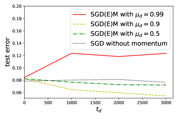
Refer to caption
Figure 6: Test error of logistic regression for notMNIST dataset.
Refer to caption
Figure 7: Test accuracy of logistic regression for notMNIST dataset.
Refer to caption
Figure 8: Test error of logistic regression for MNIST dataset.
Refer to caption
Figure 9: Test accuracy of logistic regression for MNIST dataset.

We now study the performance of SGDEM for a smooth and strongly convex loss function. We train a logistic regression model with the weight decay regularization using SGDEM for binary classification on the two-class notMNIST and MNIST datasets that contain the images from letter classes “C” and “J”, and digit classes “2” and “9”, respectively. We set the step-size α=0.01𝛼0.01\alpha=0.01. The weight decay coefficient and the minibatch size are set to 0.001 and 10, respectively. We use 100 SGDEM realizations to evaluate the average performance.

We plot the test error and test accuracy versus tdsubscript𝑡𝑑t_{d} under SGDEM for the notMNIST dataset in Figs. 6 and 7, respectively. We show the same performance measures for the MNIST dataset in Figs. 8 and 9 respectively. We observe that, unlike the case of nonconvex loss functions, it does not hurt to add momentum for the entire training. In the following, we focus on SGDM with the classical momentum update rule for a smooth and strongly convex loss function for the notMNIST dataset.
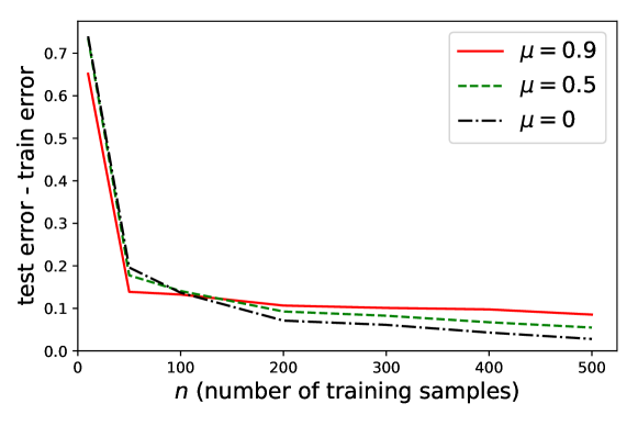
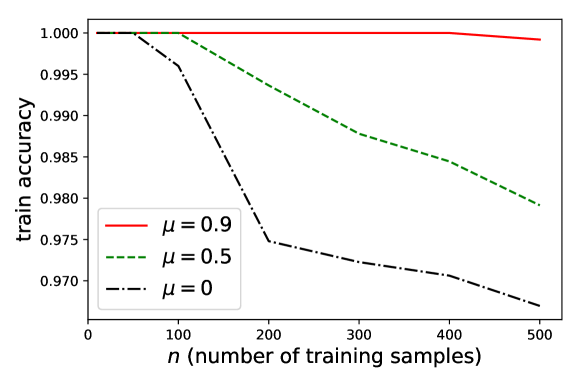
Refer to caption
Figure 10: Generalization error (cross entropy) of logistic regression for notMNIST dataset with T=1000𝑇1000T=1000 iterations.
Refer to caption
Figure 11: Training accuracy of logistic regression for notMNIST dataset with T=1000𝑇1000T=1000 iterations.

In the following, we focus on SGDM with the classical momentum update rule for a smooth and strongly convex loss function on notMINIST.

We compare the training and generalization performance of SGD without momentum with that of SGDM under μ=0.5𝜇0.5\mu=0.5 and μ=0.9𝜇0.9\mu=0.9, which are common momentum values used in practice (Goodfellow et al., 2016, Section 8.3.2).

We show in Fig. 10 the generalization error (w.r.t. cross entropy) versus the number of training samples, n𝑛n, under SGDM with fixed T=1000𝑇1000T=1000 iterations for μ=0,0.5,0.9𝜇00.50.9\mu=0,0.5,0.9. In Fig. 11, we plot the training accuracy as a function of the number of training samples for the same dataset. First, we observe that the generalization error decreases as n𝑛n increases for all values of μ𝜇\mu, which is also suggested by our stability upper bound in Theorem 18. In addition, for sufficiently large n𝑛n, we observe that the generalization error increases with μ𝜇\mu, consistent with Theorem 18. The training accuracy also improves by adding momentum as illustrated in Fig. 11.
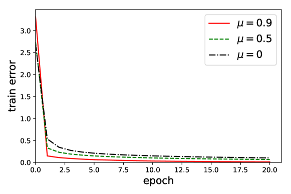
Refer to caption
Figure 12: Training error (cross entropy) of logistic regression for notMNIST dataset with n=500𝑛500n=500.
Refer to caption
Figure 13: Test error (cross entropy) of logistic regression for notMNIST dataset with n=500𝑛500n=500.
Refer to caption
Figure 14: Training accuracy of logistic regression for notMNIST dataset with n=500𝑛500n=500.

In order to study the optimization error of SGDM, we show in Figs. 12 and 13, the training error and test error, respectively, versus the number of epochs, under SGDM trained with n=500𝑛500n=500 samples. We plot the classification accuracy for training dataset in Fig. 14. We observe that the training error decreases as the number of epochs increases for all values of μ𝜇\mu, which is consistent with the convergence analysis in Theorem 35. Furthermore, as expected, we see that adding momentum improves the training error and accuracy. However, as the number of epochs increases, we note that the benefit of momentum on the test error becomes negligible. This happens because adding momentum also results in a higher generalization error thus offsetting the gain in training error.


References

  • Abramowitz and Stegun (1972) Milton Abramowitz and Irene A. Stegun. Handbook of Mathematical Functions with Formulas, Graphs, and Mathematical Tables. New York, USA: Dover, 1972.
  • Assran and Rabbat (2020) Mahmoud Assran and Michael Rabbat. On the convergence of Nesterov’s accelerated gradient method in stochastic settings. In International Conference on Machine Learning (ICML), 2020.
  • Attia and Koren (2021) Amit Attia and Tomer Koren. The instability of accelerated gradient descent. In Advances in Neural Information Processing Systems (NeurIPS), 2021.
  • Bartlett et al. (2002) Peter L Bartlett, Olivier Bousquet, and Shahar Mendelson. Localized rademacher complexities. In Conference on Learning Theory (COLT), 2002.
  • Bousquet and Elisseeff (2002) Olivier Bousquet and André Elisseeff. Stability and generalization. Journal of Machine Learning Research (JMLR), 2:499–526, 2002.
  • Bousquet et al. (2020) Olivier Bousquet, Yegor Klochkov, and Nikita Zhivotovskiy. Sharper bounds for uniformly stable algorithms. In Conference on Learning Theory (COLT), 2020.
  • Bubeck (2015) Sébastien Bubeck. Convex optimization: Algorithms and complexity. Foundations and Trends® in Machine Learning, 8(3-4):231–357, 2015.
  • Can et al. (2019) Bugra Can, Mert Gürbüzbalaban, and Lingjiong Zhu. Accelerated linear convergence of stochastic momentum methods in Wasserstein distances. In International Conference on Machine Learning (ICML), 2019.
  • (9) Yuansi Chen, Chi Jin, and Bin Yu. Stability and convergence trade-off of iterative optimization algorithms. arXiv preprint arXiv:1804.01619.
  • Chiani et al. (2003) Marco Chiani, Davide Dardari, and Marvin K. Simon. New exponential bounds and approximations for the computation of error probability in fading channels. IEEE Transactions on Wireless Communications, 2(4):840–845, 2003.
  • Clevert et al. (2016) Djork-Arné Clevert, Thomas Unterthiner, and Sepp Hochreiter. Fast and accurate deep network learning by exponential linear units (ELUs). In International Conference on Learning Representations (ICLR), 2016.
  • Deng et al. (2009) Jia Deng, Wei Dong, Richard Socher, Li-Jia Li, Kai Li, and Li Fei-Fei. ImageNet: A large-scale hierarchical image database. In Conference on Computer Vision and Pattern Recognition (CVPR), 2009.
  • Dugas et al. (2000) Charles Dugas, Yoshua Bengio, François Bélisle, Claude Nadeau, and René Garcia. Incorporating second-order functional knowledge for better option pricing. In Advances in Neural Information Processing Systems (NeurIPS), 2000.
  • Feldman and Vondrak (2018) Vitaly Feldman and Jan Vondrak. Generalization bounds for uniformly stable algorithms. In Advances in Neural Information Processing Systems (NeurIPS), 2018.
  • Feldman and Vondrak (2019) Vitaly Feldman and Jan Vondrak. High probability generalization bounds for uniformly stable algorithms with nearly optimal rate. In Conference on Learning Theory (COLT), 2019.
  • Gadat et al. (2018) Sébastien Gadat, Fabien Panloup, and Sofiane Saadane. Stochastic heavy ball. Electronic Journal of Statistics, 12(1):461–529, 2018.
  • Ghadimi et al. (2015) Euhanna Ghadimi, Hamid Reza Feyzmahdavian, and Mikael Johansson. Global convergence of the heavy-ball method for convex optimization. In European Control Conference (ECC), 2015.
  • Glorot and Bengio (2010) Xavier Glorot and Yoshua Bengio. Understanding the difficulty of training deep feedforward neural networks. In International Conference on Artificial Intelligence and Statistics (AISTATS), 2010.
  • Goodfellow et al. (2016) Ian Goodfellow, Yoshua Bengio, and Aaron Courville. Deep Learning. Cambridge, USA: The MIT Press, 2016.
  • Gradshteyn and Ryzhik (2014) Izrail Solomonovich Gradshteyn and Iosif Moiseevich Ryzhik. Table of Integrals, Series, and Products. Academic press, 2014.
  • Hardt et al. (2016) Moritz Hardt, Ben Recht, and Yoram Singer. Train faster, generalize better: Stability of stochastic gradient descent. In International Conference on Machine Learning (ICML), 2016.
  • He et al. (2016) Kaiming He, Xiangyu Zhang, Shaoqing Ren, and Jian Sun. Deep residual learning for image recognition. In Conference on Computer Vision and Pattern Recognition (CVPR), 2016.
  • (23) Dan Hendrycks and Kevin Gimpel. Gaussian error linear units (GELUs). arXiv preprint arXiv:1606.08415.
  • Kakade et al. (2008) Sham M. Kakade, Karthik Sridharan, and Ambuj Tewari. On the complexity of linear prediction: risk bounds, margin bounds, and regularization. In Advances in Neural Information Processing Systems (NeurIPS), 2008.
  • (25) Nitish Shirish Keskar and Richard Socher. Improving generalization performance by switching from Adam to SGD. arXiv preprint arXiv:1712.07628.
  • Kingma and Ba (2015) Diederik P. Kingma and Jimmy Ba. Adam: A method for stochastic optimization. In International Conference on Learning Representations (ICLR), 2015.
  • Klochkov and Zhivotovskiy (2021) Yegor Klochkov and Nikita Zhivotovskiy. Stability and deviation optimal risk bounds with convergence rate O(1/n)𝑂1𝑛O(1/n). In Advances in Neural Information Processing Systems (NeurIPS), 2021.
  • (28) Alex Krizhevsky. Learning multiple layers of features from tiny images. Technical report, University of Toronto, 2009.
  • Krizhevsky et al. (2012) Alex Krizhevsky, Ilya Sutskever, and Geoffrey E. Hinton. ImageNet classification with deep convolutional neural networks. In Advances in Neural Information Processing Systems (NeurIPS), 2012.
  • Laborde and Oberman (2020) Maxime Laborde and Adam Oberman. A Lyapunov analysis for accelerated gradient methods: from deterministic to stochastic case. In International Conference on Artificial Intelligence and Statistics (AISTATS), 2020.
  • Lessard et al. (2016) Laurent Lessard, Benjamin Recht, and Andrew Packard. Analysis and design of optimization algorithms via integral quadratic constraints. SIAM Journal on Optimization, 26(1):57–95, 2016.
  • Li and Orabona (2020) Xiaoyu Li and Francesco Orabona. A high probability analysis of adaptive SGD with momentum. arXiv preprint arXiv:2007.14294, 2020.
  • Needell et al. (2014) Deanna Needell, Nati Srebro, and Rachel Ward. Stochastic gradient descent, weighted sampling, and the randomized Kaczmarz algorithm. In Advances in Neural Information Processing Systems (NeurIPS), 2014.
  • Nemirovskij and Yudin (1983) Arkadij Nemirovskij and David Borisovich Yudin. Problem Complexity and Method Efficiency in Optimization. Wiley-Interscience, 1983.
  • Nesterov (1983) Yurii Nesterov. A method of solving a convex programming problem with convergence O(1/k2)𝑂1superscript𝑘2O(1/k^{2}). Doklady Akademii Nauk, 269(3):543–547, 1983.
  • Ochs et al. (2014) Peter Ochs, Yunjin Chen, Thomas Brox, and Thomas Pock. iPiano: Inertial proximal algorithm for nonconvex optimization. SIAM Journal on Imaging Sciences, 7(2):1388–1419, 2014.
  • Ochs et al. (2015) Peter Ochs, Thomas Brox, and Thomas Pock. iPiasco: Inertial proximal algorithm for strongly convex optimization. Journal of Mathematical Imaging and Vision, 53(2):171–181, 2015.
  • Ong (2017) Ming Yang Ong. Understanding generalization. 2017. Thesis available at https://dspace.mit.edu/bitstream/handle/1721.1/113119/1016455698-MIT.pdf?sequence=1.
  • Orvieto et al. (2020) Antonio Orvieto, Jonas Kohler, and Aurelien Lucchi. The role of memory in stochastic optimization. In Conference on Uncertainty in Artificial Intelligence (UAI), 2020.
  • Polyak (1964) Boris T. Polyak. Some methods of speeding up the convergence of iteration methods. USSR Computational Mathematics and Mathematical Physics, 4(5):1–17, 1964.
  • Rockafellar (1976) R. Tyrrell Rockafellar. Monotone operators and the proximal point algorithm. SIAM Journal on Control and Optimization, 14(5):877–898, 1976.
  • Rumelhart et al. (1986) David E. Rumelhart, Geoffrey E. Hinton, and Ronald J. Williams. Learning representations by backpropagating errors. Nature, 323(6088):533–536, 1986.
  • Shalev-Shwartz and Ben-David (2014) Shai Shalev-Shwartz and Shai Ben-David. Understanding Machine Learning: From Theory to Algorithms. Cambridge University Press, 2014.
  • Shalev-Shwartz et al. (2010) Shai Shalev-Shwartz, Ohad Shamir, Nathan Srebro, and Karthik Sridharan. Learnability, stability and uniform convergence. Journal of Machine Learning Research (JMLR), 11:2635–2670, 2010.
  • Sridharan et al. (2008) Karthik Sridharan, Shai Shalev-Shwartz, and Nathan Srebro. Fast rates for regularized objectives. In Advances in Neural Information Processing Systems (NeurIPS), 2008.
  • Su et al. (2014) Weijie Su, Stephen Boyd, and Emmanuel Candès. A differential equation for modeling Nesterov’s acceleratedgradient method: Theory and insights. In Advances in Neural Information Processing Systems (NeurIPS), 2014.
  • Sutskever et al. (2013) Ilya Sutskever, James Martens, George Dahl, and Geoffrey E. Hinton. On the importance of initialization and momentum in deep learning. In International Conference on Machine Learning (ICML), 2013.
  • Valiant (1984) Leslie G. Valiant. A theory of the learnable. Communications of the ACM, 27(11):1134–1142, 1984.
  • Vapnik and Chervonenkis (1971) Vladimir N. Vapnik and Alexey Ya Chervonenkis. On the uniform convergence of relative frequencies of events to their probabilities. Theory of Probability and Its Applications, 16(2):264–280, 1971.
  • Wilson et al. (2017) Ashia C. Wilson, Rebecca Roelofs, Mitchell Stern, Nati Srebro, and Benjamin Recht. The marginal value of adaptive gradient methods in machine learning. In Advances in Neural Information Processing Systems (NeurIPS), 2017.
  • Wilson et al. (2021) Ashia C. Wilson, Ben Recht, and Michael I. Jordan. A Lyapunov analysis of momentum methods in optimization. Journal of Machine Learning Research (JMLR), 22:34–1, 2021.
  • (52) Bing Xu, Naiyan Wang, Tianqi Chen, and Mu Li. Empirical evaluation of rectified activations in convolutional network. arXiv preprint arXiv:1505.00853v2.
  • Yan et al. (2018) Yan Yan, Tianbao Yang, Zhe Li, Qihang Lin, and Yi Yang. A unified analysis of stochastic momentum methods for deep learning. In International Joint Conferences on Artificial Intelligence (IJCAI), 2018.