Synchronization of stochastic hybrid oscillators driven by a common switching environment

Abstract

Many systems in biology, physics and chemistry can be modeled through ordinary differential equations, which are piecewise smooth, but switch between different states according to a Markov jump process. In the fast switching limit, the dynamics converges to a deterministic ODE. In this paper we suppose that this limit ODE supports a stable limit cycle. We demonstrate that a set of such oscillators can synchronize when they are uncoupled, but they share the same switching Markov jump process. The latter is taken to represent the effect of a common randomly switching environment. We determine the leading order of the Lyapunov coefficient governing the rate of decay of the phase difference in the fast switching limit. The analysis bears some similarities to the classical analysis of synchronization of stochastic oscillators subject to common white noise. However the discrete nature of the Markov jump process raises some difficulties: in fact we find that the Lyapunov coefficient from the quasi-steady-state approximation differs from the Lyapunov coefficient one obtains from a second order perturbation expansion in the waiting time between jumps. Finally, we demonstrate synchronization numerically in the radial isochron clock model and show that the latter Lyapinov exponent is more accurate.

There are a growing number of systems in physics and biology where a population of oscillators can be synchronized by a randomly fluctuating external input applied globally to all of the oscillators, even if there are no interactions between the oscillators (noise-induced phase synchronization). Experimental evidence for such an effect has been found in neural oscillations of the olfactory bulb, synthetic genetic oscillators, laser dynamics, and variations in geographically separated animal populations. Most previous studies of noise-induced phase synchronization have taken the oscillators to be driven by common Gaussian noise. Typically, phase synchronization is established by constructing the Lyapunov exponent for the dynamics of the phase difference between a pair of oscillators and averaging with respect to the noise. If the averaged Lyapunov exponent is negative definite, then the phase difference is expected to decay to zero in the large time limit, establishing phase synchronization. In this paper we extend the theory of noise-induced synchronization to the case of a common randomly switching environment. Each oscillator then evolves according to a piecewise deterministic Markov process, which involves the coupling between a piecewise continuous differential equation and a time-homogeneous Markov chain. In the fast switching limit, the dynamics converges to a deterministic ODE, which is assumed to support a stable limit cycle. We demonstrate that an uncoupled population of such oscillators can synchronize when they share the same switching Markov jump process. We determine the leading order of the Lyapunov coefficient governing the rate of decay of the phase differences in the weak noise regime (fast but finite switching rates), and show that it differs from the standard expression obtained using a Gaussian approximation of the noise.

 

I Introduction

Self–sustained oscillations in biological, physical and chemical systems are often described in terms of limit cycle oscillators where the timing along each limit cycle is specified in terms of a single phase variable. Phase reduction methods can then be used to analyze synchronization of an ensemble of weakly-coupled oscillators by approximating the high–dimensional limit cycle dynamics as a closed system of equations for the corresponding phase variables Winfree80 ; Kuramoto84 ; Erm84 ; Glass88 ; Erm91 ; Erm96 ; Holmes04 ; Ashwin16 ; Nakao16 . More recently, there has been considerable interest in applying phase reduction methods to the analysis of noise-induced phase synchronization Teramae04 ; Goldobin05 ; Nakao07 ; Yoshimura08 ; Teramae09 ; Ly09 ; Erm10 . This concerns the observation that a population of oscillators can be synchronized by a randomly fluctuating external input applied globally to all of the oscillators, even if there are no interactions between the oscillators. Evidence for such an effect has been found in experimental studies of neural oscillations in the olfactory bulb Galan08 , and the synchronization of synthetic genetic oscillators Zhou08 ; Paulsson16 . A related phenomenon is the reproducibility of a dynamical system’s response when repetitively driven by the same fluctuating input, even though initial conditions vary across trials. Examples include the spike-time reliability of single neurons Mainen95 ; Galan06 , improvements in the reproducibility of laser dynamics Uchida04 , and synchronized variations in wild animal populations located in distinct, well-separated areas caused by common environmental fluctuations Grenfell98 .

Most studies of noise-induced synchronization take the oscillators to be driven by common Gaussian noise. Typically, phase synchronization is established by constructing the Lyapunov exponent for the dynamics of the phase difference between a pair of oscillators and averaging with respect to the noise. If the averaged Lyapunov exponent is negative definite, then the phase difference is expected to decay to zero in the large time limit, establishing phase synchronization. However, it has also been shown that common Poisson-distributed random impulses, dichotomous or telegrapher noise, and other types of noise generally induce synchronization of limit-cycle oscillators Nakao05 ; Nagai05 ; Goldobin10 . Consider, in particular, the case of an additive dichotomous noise signal $I(t)$ driving a population of $M$ identical non-interacting oscillators according to the system of equations $\dot{x}_{j}=F(x_{j})+I(t)$, where $x_{j}\in\mathbb{R}^{d}$ is the state of the $j$th oscillator, $j=1,\ldots,M$ Nagai05 , see Fig. 1. Here $I(t)$ switches between two values $I_{0}$ and $I_{1}$ at random times generated by a two-state Markov chain Bena06 . That is, $I(t)=I_{0}(1-N(t))+I_{1}N(t)$ for $N(t)\in\{0,1\}$, with the time $T$ between switching events taken to be exponentially distributed with mean switching time $\tau$. Suppose that each oscillator supports a stable limit cycle for each of the two input values $I_{0}$ and $I_{1}$. It follows that the internal state of each oscillator randomly jumps between the two limit cycles. Nagai et al Nagai05 show that in the slow switching limit (large $\tau$), the dynamics can be described by random phase maps. Moreover, if the phase maps are monotonic, then the associated Lyapunov exponent is generally negative and phase synchronization is stable.

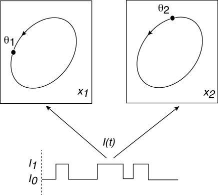
Figure 1: Pair of non-interacting limit cycle oscillators with phases $\theta_{j}(t)$, $j=1,2$, driven by a common switching external input $I(t)$

The dichotomous noise-driven system is just one example of a much more general class of randomly switching processes known as piecewise deterministic Markov processes (PDMPs) Davis84 ; Bressloff17 . More explicitly, let $N(t)\in\Gamma\equiv\{0,\cdots,\Lambda_{0}-1\}$ denote the state of the randomly switching environment. When the environmental state is $N(t)=n$, each oscillator $x_{i}(t)$ evolves according to the piecewise deterministic ordinary differential equation (ODE) $\dot{x_{i}}=F_{n}(x_{i}),\quad i=1,\ldots,M$, where the vector field $F_{n}:\mathbb{R}^{d}\to\mathbb{R}^{d}$ is a smooth function. The discrete stochastic variable $N(t)$ evolves according to a stationary, continuous-time Markov chain with transition matrix ${\bf W}$. The additive dichotomous noise case is recovered by taking $\Lambda_{0}=2$ and $F_{n}(x)=F(x)+I_{n}$. One major application of PDMPs is to stochastic gene regulatory networks, where the continuous variables $x_{j}$ are the concentrations of protein products (and possibly mRNAs) and the discrete variables represent the various activation/inactivation states of the genes Kepler01 ; Bose04 ; Zeiser08 ; Smiley10 ; Paulsson11 ; Newby12 ; Singh14 ; Koeppl14 ; Newby15 ; Hufton16 ; Levien18 . The common randomly switching environment could represent the state of a promoter site that is common to a pair of genes within the same cell, or the state of the extracellular environment that drives gene expression in a population of cells. It is thought that synchronous oscillations may have an important functional purpose in systems biology Paulsson11

In this paper we develop the theory of noise-induced synchronization for a population of non-interacting PDMPs evolving under a common randomly switching environment. (The population model is presented in section II). In the slow switching limit one could generalize the approach of Nagai et al Nagai05 by assuming that each of the vector fields $F_{n}(x_{i})$, $n\in\Gamma$, supports a stable limit cycle and constructing the associated random phase maps. Here, instead, we consider the fast switching regime in which the transition rates between the discrete states $n\in\Gamma$ are much faster than the relaxation rates of the piecewise deterministic dynamics for $x_{i}\in\mathbb{R}^{d}$. Thus there is a separation of time scales between the discrete and continuous processes, so that if $R$ is the characteristic relaxation rate of the continuous dynamics, then $r/\epsilon$ is the characteristic transition rate of the Markov chain for some small positive dimensionless parameter $\epsilon$. If the Markov chain is ergodic, then in the fast switching or adiabatic limit $\epsilon\rightarrow 0$ one obtains a deterministic dynamical system in which one averages the piecewise dynamics with respect to the corresponding unique stationary distribution. Suppose that in the deterministic limit we have a population of independent limit cycle oscillators. Since there is no coupling or remaining external drive to the oscillators, their phases are uncorrelated. The basic issue we wish to address is whether or not phase synchronization occurs when $\epsilon>0$; we will refer to the resulting oscillators as stochastic hybrid limit cycle oscillators. We will proceed by constructing the Lyapunov exponent for a pair of such oscillators driven by a common randomly switching environment.

In section III we obtain an approximate expression for the Lyapunov exponent by considering a quasi-steady-state (QSS) diffusion approximation of the underlying PDMPs Newby10a (see also appendix A), in which each oscillator is approximated by a stochastic differential equation (SDE) with a common Gaussian input. This allows us to adapt previous work on the phase reduction of stochastic limit cycle oscillators Teramae04 ; Goldobin05 ; Nakao07 ; Teramae09 , and thus establish that phase synchronization occurs under the diffusion approximation. However, the QSS approximation is only intended to be accurate over timescales that are longer than $O(\epsilon)$. Hence, it is unclear whether or not the associated Lyapunov exponent is accurate, since it is obtained from averaging the fluctuations in the noise over infinitesimally small timescales. Therefore, in section IV we derive a more accurate expression for the Lyapunov exponent by working directly with an exact implicit equation for the phase dynamics. We exploit the fact that multiple switching events (jumps) occur during small excursions around the limit cycle for small $\epsilon$, which allows us to express the Lyapunov exponent in terms of discrete sums over these events. Taking expectations then yields an expression for the Lyapunov exponent that differs significantly from the one obtained using the diffusion approximation. Note, however, that both are negative definite, so they both imply phase synchronization but at different rates. Our derivation of the Lyapunov exponent from the exact phase equation also allows us to obtain greater insights into the nature of the QSS approximation and the meaning of the associated Brownian motion (see also appendix B). Finally, we illustrate the theory by considering the particular example of radial isochron clocks (section V).

II Population of stochastic hybrid limit cycle oscillators

Consider a population of identical, noninteracting dynamical systems labeled $i=1,\ldots,M$, whose states are described by the pair $(x_{i}(t),N(t))\in\Sigma\times\Gamma$, where $x_{i}(t)$ is a continuous variable in a connected bounded domain $\Sigma\subset\mathbb{R}^{d}$ and $N(t)$ is an $i$-independent discrete stochastic variable taking values in the finite set $\Gamma\equiv\{0,\cdots,\Lambda_{0}-1\}$. The latter represents the state of an environment that is common to all members of the population. When the environmental state is $N(t)=n$, $x_{i}(t)$ evolves according to the piecewise deterministic ODE

$$\dot{x_{i}}=F_{n}(x_{i}),\quad i=1,\ldots,M,$$ (2.1)

where the vector field $F_{n}:\mathbb{R}^{d}\to\mathbb{R}^{d}$ is a smooth function. We assume that the dynamics of $x_{i}$ is confined to the domain $\Sigma$. The discrete stochastic variable is taken to evolve according to a homogeneous, continuous-time Markov chain with $x$-independent generator ${\bf A}$, where

$$A_{nm}=W_{nm}-\delta_{n,m}\sum_{k\in\Gamma}W_{kn},$$

and ${\bf W}$ is the transition matrix. We make the further assumption that the chain is irreducible, that is, there is a non-zero probability of transitioning, possibly in more than one step, from any state to any other state of the Markov chain. This implies the existence of a unique invariant probability distribution on $\Gamma$, denoted by $\rho$, such that

$$\sum_{m\in\Gamma}A_{nm}\rho_{m}=0,\quad\forall n\in\Gamma.$$ (2.2)

As a simple example, suppose that $N(t)$ evolves according to a two-state Markov chain. That is, $N(t)\in\Gamma\equiv\{0,1\}$ and the generator of the Markov chain is given by the matrix

$${\bf A}=\left(\begin{array}[]{cc}-k_{-}&k_{+}\\ k_{-}&-k_{+}\end{array}\right).$$ (2.3)

The corresponding stationary distribution of the Markov chain then has components

$$\rho_{0}=\frac{k_{+}}{k_{+}+k_{-}},\quad\rho_{1}=\frac{k_{-}}{k_{+}+k_{-}}.$$ (2.4)

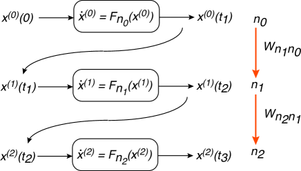
Figure 2: Schematic diagram of a PDMP for a sequence of jump times $\{t_{1},\ldots\}$, and a corresponding set of discrete states $\{n_{0},n_{1},\ldots\}$. See text for details

Eq. (2.1) defines a PDMP Davis84 on $\mathbb{R}^{d}$ for each $i=1,\ldots,M$, also known as a stochastic hybrid system (SHS). A useful way to implement the PDMP is to decompose the transition matrix of the Markov chain as $W_{nm}=P_{nm}\lambda_{m}$, with $\sum_{n\neq m}P_{nm}=1$. Here $\lambda_{m}$ is the rate of the exponential waiting time density for transitions from state $m$, whereas $P_{nm}$ is the probability of the transition $m\rightarrow n$, $n\neq m$. Suppose that $N(t)=n_{0}$ and let $t_{1}$ be an exponentially distributed random variable with rate $\lambda_{n_{0}}$. That is,

$$\mathbb{P}(t_{1}<t)=1-\exp\left(-\lambda_{n_{0}}t\right).$$

Then in the random time interval $s\in[0,\,t_{1})$ the state of the $i$th system is $(x^{(0}(s),n_{0})$ with $x^{(0)}$ evolving according to Eq. (2.1) for $n=n_{0}$. (For the moment, we drop the population label $i$.) At the random time $t_{1}$ we choose an internal state $n_{1}\in\Gamma$ with probability $P_{n_{1}n_{0}}$, and call $x^{(1)}(t)$ the solution of the following Cauchy problem on $[t_{1},\infty)$:

$$\left\{\begin{array}[]{lcl}\dot{x}^{(1)}(t)&=&F_{n_{1}}(x^{(1)}(t),\quad t\geq t_{1}\\ x^{(1)}(t_{1})&=&x^{(0)}(t_{1})\end{array}\right.$$

Iterating this procedure, we construct a sequence of increasing jumping times $(t_{k})_{k\geq 0}$ (setting $t_{0}=0$) and a corresponding sequence of internal states $(n_{k})_{k\geq 0}$. The evolution $(x(t),\,N(t))$ is then defined as, see Fig. 2

$$(x(t),N(t))=(x^{(k)}(t),n_{k})\quad\mbox{if}\ t_{k}\leq t<t_{k+1}.$$ (2.5)

Introduce the population vector ${\bf x}(t)=(x_{1}(t),\ldots,x_{M}(t))$ and define the probability density $p_{n}({\bf x},t)$, given the initial conditions $x_{i}(0)=x_{i,0},N(0)=n_{0}$, according to

$$p_{n}({\bf x},t)d{\bf x}=\mathbb{P}\{{\bf x}(t)\in({\bf x},{\bf x}+d{\bf x}),\,N(t)=n|{\bf x}_{0},n_{0}\}.$$

It can be shown that $p$ evolves according to the forward differential Chapman-Kolmogorov (CK) equation Gardiner09 ; Bressloff17

$$\frac{\partial p_{n}}{\partial t}={\mathbb{L}}p_{n},$$ (2.6)

with the generator ${\mathbb{L}}$ defined according to

$${\mathbb{L}}p_{n}({\bf x},t)=-\sum_{i=1}^{M}\nabla_{i}\cdot\left[F_{n}(x_{i})p_{n}({\bf x},t)\right]+\frac{1}{\epsilon}\sum_{m\in\Gamma}A_{nm}p_{m}({\bf x},t).$$ (2.7)

Here $\nabla_{i}$ denotes the $d$-dimensional gradient operator with respect to $x_{i}$. The first term on the right-hand side represents the probability flow associated with the piecewise deterministic dynamics for a given $n$, whereas the second term represents jumps in the discrete state $n$. Note that we have rescaled the matrix ${\bf A}$ by introducing the dimensionless parameter $\epsilon$, $\epsilon>0$. This is motivated by the observation that many applications of PDMPs involve a separation of time-scales between the relaxation time for the dynamics of the continuous variables $x$ and the rate of switching between the different discrete states $n$ of the environment. The fast switching limit then corresponds to the case $\epsilon\rightarrow 0$. Now introduce the averaged vector field $\overline{F}:\mathbb{R}^{d}\to\mathbb{R}^{d}$ by

$$\overline{F}(x)=\sum_{n\in\Gamma}\rho_{n}F_{n}(x)$$ (2.8)

and define the averaged system

$$\left\{\begin{array}[]{lcl}\dot{x_{i}}(t)&=&\overline{F}(x_{i}(t)),\quad i=1,\ldots,M,\\ x_{i}(0)&=&x_{0}\end{array}\right.$$ (2.9)

Intuitively speaking, one expects the PDMP (2.1) to reduce to the deterministic dynamical system (2.9) in the fast switching limit $\epsilon\rightarrow 0$. That is, for sufficiently small $\epsilon$, the Markov chain undergoes many jumps over a small time interval $\Delta t$ during which $\Delta x\approx 0$, and thus the relative frequency of each discrete state $n$ is approximately $\rho_{n}$. This can be made precise in terms of a law of large numbers for PDMPs proven in Faggionato10 .

In the fast switching (deterministic) limit, each member of the population becomes independent, since the dependence on the current state of the environment disappears. In this paper, we will assume that for each $i=1,\ldots,M$, the averaged dynamical system (2.9) supports a set of stable periodic solutions with the same natural frequency $\overline{\omega}=2\pi/\overline{\Delta}$. That is, we have a population of identical, independent oscillators in the fast switching limit. In state space, each periodic solution is an isolated attractive trajectory or limit cycle. The dynamics on the limit cycle can be described by a uniformly rotating phase such that

$$\frac{d\theta_{i}}{dt}=\overline{\omega},$$ (2.10)

and $x_{i}={\Phi}(\theta_{i}(t))=\Phi(\overline{\omega}t+\psi_{i})$ with ${\Phi}$ a $2\pi$-periodic function and $\psi_{i}$ the initial phase. Note that $\Phi$ satisfies the equation

$$\overline{\omega}\frac{d\Phi}{d\theta}=\overline{F}(\Phi(\theta)).$$ (2.11)

Differentiating both sides with respect to $\theta$ gives

$$\frac{d}{d\theta}\left(\frac{d\Phi}{d\theta}\right)=\overline{\omega}^{-1}\overline{J}(\theta)\cdot\frac{d\Phi}{d\theta},$$ (2.12)

where $\overline{J}$ is the $2\pi$-periodic Jacobian matrix

$$\overline{J}_{ab}(\theta)\equiv\left.\frac{\partial\overline{F}_{a}}{\partial x_{b}}\right|_{x=\Phi(\theta)}$$ (2.13)

for $a,b=1,\ldots,d$.

In the deterministic limit, there is no mechanism for phase synchronizing the population of oscillators, since $\theta_{j}(t)-\theta_{i}(t)=\psi_{j}-\psi_{i}$ for all $t$. The main issue we wish to address in this paper is whether or not the presence of a common switching environment can synchronize the population of stochastic hybrid oscillators when $\epsilon>0$, analogous to the noise-driven synchronization of SDEs Teramae04 ; Goldobin05 ; Nakao07 ; Yoshimura08 ; Teramae09 .

III Diffusion approximation and phase SDE

One approach to analyzing synchronization in the fast switching regime ($0<\epsilon\ll 1$) is to use a QSS diffusion or adiabatic approximation, in which the CK Eq. (2.6) is approximated by a Fokker-Planck (FP) equation for the total density $C({\bf x},t)=\sum_{n}p_{n}({\bf x},t)$ Newby10a . The latter determines the probability distribution of solutions of a corresponding SDE for a population of oscillators driven by a common $O(\sqrt{\epsilon})$ multiplicative noise term, which can then be reduced to an effective SDE for the phases along the lines of Ref. Teramae04 . The resulting FP equation in the Stratonovich representation takes the form (see appendix A)

$$\frac{\partial C}{\partial t} =-\sum_{i=1}^{M}\nabla_{i}\cdot\left[\overline{F}(x_{i})C\right]$$ (3.1a)

$$-\epsilon\sum_{i,j=1}^{M}\sum_{m,n\in\Gamma}A_{mn}^{\dagger}\rho_{n}\nabla_{i}\cdot\left[G_{m}(x_{i})\nabla_{j}\cdot(G_{n}(x_{j})C)\right],$$

with

$$G_{m}(x) = F_{m}(x)-\overline{F}(x).$$ (3.1b)

Since Eq. (3.1a) is symmetric with respect to the exchange $(ni,mj)\leftrightarrow(mj,ni)$ we can replace ${\bf A}\rho$ by its symmetric part

$$\tilde{A}_{mn}=\frac{1}{2}(A^{\dagger}_{mn}\rho_{n}+A^{\dagger}_{nm}\rho_{m}).$$ (3.2)

Note that the matrix $\tilde{\bf A}$ is negative definite, as we demonstrate in the Appendix. For example, in the case of a two-state Markov chain, $\tilde{\bf A}=\mbox{diag}(-\rho_{0}/(k_{+}+k_{-}),-\rho_{1}/(k_{+}+k_{-}))$

It follows that under the diffusion approximation, the PDMP (2.1) can be approximated by the Stratonovich SDE

$$dX_{i}(t)=\overline{F}(X_{i})dt+\sqrt{2\epsilon}\sum_{m,n\in\Gamma}G_{m}(X_{i})B_{mn}dW_{n}(t)$$ (3.3)

for $i=1,\ldots,M$, where ${\bf B}{\bf B}^{\top}=-\tilde{\bf A}$, and $W(t)$ is a vector of uncorrelated Brownian motions in $\mathbb{R}^{M}$,

$$\mathbb{E}\big{[}{\bf W}(t){\bf W}(t)^{\top}\big{]}=t{\bf I},$$

and ${\bf I}$ is the identity matrix. (Note that it doesn’t matter which Hermitian square root of $-\tilde{\bf A}$ we take for ${\bf B}$, since they all yield the same statistical behavior of $X_{i}(t)$.) Eq. (3.3) represents a population of independent, non-interacting limit cycle oscillators, driven by common external white noise. One can now use phase reduction methods developed for SDEs.

III.1 Phase reduction

First, suppose that the noise amplitude $\epsilon$ is sufficiently small relative to the rate of attraction to the limit cycle, so that deviations transverse to the limit cycle are also small (up to some exponentially large stopping time). This suggests that the definition of a phase variable persists in the stochastic setting, and one can derive a stochastic phase equation by decomposing the solution to the SDE (3.3) according to

$$X_{i}(t)=\Phi(\theta_{i}(t))+\sqrt{\epsilon}v_{i}(t),$$ (3.4)

with $\theta_{i}(t)$ and $v_{i}(t)$ corresponding to the phase and amplitude components, respectively, of the $i$th oscillator. However, there is not a unique way to define the phase $\theta_{i}$, which reflects the fact that there are different ways of projecting the exact solution onto the limit cycle Gonze02 ; Koeppl11 ; Bonnin17 ; Maclaurin18a , see Fig. 4. One well-known approach is to use the method of isochrons Teramae04 ; Nakao07 ; Yoshimura08 ; Teramae09 , which we briefly outline here.

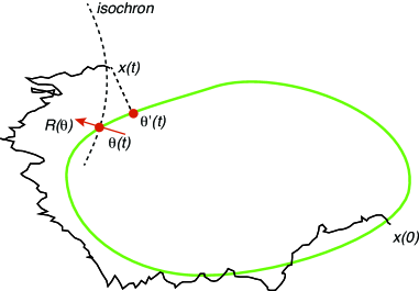
Figure 3: Different choices of amplitude-phase decomposition. Two possibilities are orthogonal projection with phase $\theta^{\prime}(t)$ and isochronal projection with phase $\theta(t)$. In the latter case, the response to perturbations depends on the phase response curve ${R}(\theta)$, which is normal to the isochron at the point of intersection with the limit cycle.

Consider the unperturbed deterministic system $\dot{x}_{i}=\overline{F}(x_{i})$. Stroboscopically observing the system at time intervals of length $\overline{\Delta}$ leads to a Poincare mapping

$$x_{i}(t)\rightarrow x_{i}(t+\overline{\Delta})\equiv{\mathcal{P}}(x_{i}(t)),$$

for which all points on the limit cycle are fixed points. Choose a point $x_{i}^{*}$ on the limit cycle and consider all points in the vicinity of $x_{i}^{*}$ that are attracted to it under the action of ${\mathcal{P}}$. They form a $(d-1)$-dimensional hypersurface ${\mathcal{I}}$ called an isochron Winfree80 ; Kuramoto84 ; Glass88 ; Erm96 ; Holmes04 , crossing the limit cycle at $x_{i}^{*}$. A unique isochron can be drawn through each point on the limit cycle (at least locally) so the isochrons can be parameterized by the phase, ${\mathcal{I}}={\mathcal{I}}(\theta_{i})$. Finally, the definition of phase is extended by taking all points $x_{i}\in{\mathcal{I}}(\theta_{i})$ to have the same phase, $\Theta(x_{i})=\theta_{i}$, which then rotates at the natural frequency $\overline{\omega}$ (in the unperturbed case). Hence, for an unperturbed oscillator in the vicinity of the limit cycle we have

$$\overline{\omega}=\frac{d\Theta(x_{i})}{dt}=\nabla\Theta(x_{i})\cdot\frac{dx_{i}}{dt}=\nabla\Theta(x_{i})\cdot F(x_{i}).$$

Now consider the Stratonovich SDE (3.3). For the moment, we replace the $O(\epsilon^{1/2})$ term by a bounded deterministic function $H\in\mathbb{R}^{d}$ so that we have the perturbed deterministic equation

$$\frac{dx_{i}}{dt}=\overline{F}(x_{i})+\sqrt{\epsilon}H(x_{i},t).$$

The additional complications arising from a stochastic perturbation will be addressed below. Differentiating the isochronal phase using the chain rule gives

$$\frac{d\Theta}{dt} =\nabla\Theta(x_{i})\cdot(\overline{F}(x_{i})+\sqrt{\epsilon}H({x_{i}},t))$$

$$=\overline{\omega}+\sqrt{\epsilon}\nabla\Theta(x_{i})\cdot H(x_{i},t).$$

We now make the approximation that deviations of $x_{i}$ from the limit cycle are ignored on the right-hand side by setting $x_{i}(t)=\Phi(\theta_{i}(t))$ with $\Phi$ the $2\pi$-periodic solution on the limit cycle. This then yields the closed phase equation

$$\frac{d\theta_{i}}{dt}=\overline{\omega}+\sqrt{\epsilon}\sum_{a=1}^{d}R_{a}(\theta_{i})H_{a}(\Phi(\theta_{i}),t),$$ (3.5)

where

$$R_{a}(\theta)=\left.\frac{\partial\Theta}{\partial x_{a}}\right|_{x_{a}=\Phi(\theta)}$$ (3.6)

is a $2\pi$-periodic function of $\theta$ known as the $a$th component of the phase resetting curve (PRC) Winfree80 ; Kuramoto84 ; Glass88 ; Erm96 ; Holmes04 . One way to evaluate the PRC is to exploit the fact that it is the $2\pi$-periodic solution of the linear equation

$$\overline{\omega}\frac{dR(\theta)}{d\theta}=-\overline{J}(\theta)^{\top}\cdot R(\theta),$$ (3.7)

under the normalization condition

$$R(\theta)\cdot\frac{d\Phi(\theta)}{d\theta}=1.$$ (3.8)

$\overline{J}(\theta)^{\top}$ is the transpose of the Jacobian matrix $\overline{J}(\theta)$.

Returning to the Stratonovich SDE (3.3), treating the stochastic perturbation along identical lines to the deterministic case, (i.e. substituting $H(t)dt=\sqrt{2}\sum_{m,n\in\Gamma}\left[F_{m}(\Phi(\theta_{i}))-\overline{F}(\Phi(\theta_{i}))\right]B_{mn}dW_{n}(t)$) and exploiting the fact that the usual rules of calculus hold (in contrast to Ito SDEs), would then lead to the following SDE for the phase $\theta_{i}(t)$:

$$d\theta_{i} =\overline{\omega}dt+\sqrt{2\epsilon}\sum_{m,n\in\Gamma}{\mathcal{F}}_{m}(\theta_{i})B_{mn}dW_{n}(t),$$ (3.9)

where

$${\mathcal{F}}_{n}(\theta_{i})=\sum_{a=1}^{d}R_{a}(\theta_{i})\left[F_{n,a}(\Phi(\theta_{i}))-\overline{F}_{a}(\Phi(\theta_{i}))\right].$$ (3.10)

Introducing the population phase vector ${\bm{\theta}}(t)=(\theta_{1}(t),\ldots,\theta_{M}(t))$, the corresponding phase FP equation for the population probability density $C({\bm{\theta}},t)$ is

$$\frac{\partial C}{\partial t} =-\overline{\omega}\sum_{i=1}^{M}\frac{\partial C}{\partial\theta_{i}}$$ (3.11)

$$+\epsilon\sum_{i,j=1}^{M}\sum_{m,n\in\Gamma}\tilde{A}_{mn}\frac{\partial}{\partial\theta_{i}}\left[{\mathcal{F}}_{m}(\theta_{i})\frac{\partial}{\partial\theta_{j}}({\mathcal{F}}_{n}(x_{j})C)\right].$$

However, there are a number of major differences from the deterministic case. Probably the most significant is that a Wiener process is not bounded, which means that over sufficiently long time intervals there is a small but non-zero probability that the stochastic term induces large deviations from the limit cycle, resulting in a breakdown of the perturbation analysis. This issue can be addressed using variational methods and large deviation theory Giacomin16 ; Maclaurin18a , which show that for sufficiently small $\epsilon$, the system remains in a neighborhood of the limit cycle up to exponentially long times. The second issue is that there are no $O(\sqrt{\epsilon})$ corrections to the deterministic part of the phase equation so that one has to go to $O(\epsilon)$ in order to determine the leading order corrections to the drift term. There are two sources of $O(\epsilon)$ terms: one arises from the coupling between the phase and amplitude fluctuations transverse to the limit cycle, and the second arises from changing between Stratonovich and Ito versions of the SDE based on Ito’s formula Teramae09 ; Giacomin16 ; Bonnin17 ; Maclaurin18a . The precise form of these terms will also depend on the particular choice of phase reduction method. However, if the limit cycle is sufficiently attracting then they tend to have a small effect Teramae09 . Moreover, such drift terms do not contribute to the leading order expression for Lyapunov exponent describing the evolution of phase differences, see below Eq. (3.16). Therefore, we shall drop such contributions in our subsequent analysis, and reinterpret Eq. (3.9) as an Ito SDE.

III.2 Lyapunov exponent

We now use the phase SDE (3.9) interpreted in the Ito sense to investigate the effects of a common switching environment in the small $\epsilon$ regime, following previous studies Teramae04 ; Nakao07 ; Yoshimura08 ; Teramae09 ; Ly09 . The first step is to consider the SDE for the phase difference $\psi=\theta_{j}-\theta_{1}$ for any fixed $j$ such that $j\neq 1$. Assuming $\psi$ is infinitesimally small, we have

$$\frac{d\psi}{dt}=\sqrt{2\epsilon}\psi(t)\left[\sum_{m,n\in\Gamma}{\mathcal{F}}^{\prime}_{m}(\phi)B_{mn}dW_{n}(t)\right],$$ (3.12)

where ^′ denotes differentiation with respect to $\phi$ and we have set $\theta_{1}(t)=\phi(t)$ so that $\phi(t)$ evolves according to Eq. (3.9) for $i=1$. Introducing a new variable $y=\log(\psi)$ and using Ito’s formula yields the SDE

$$dy =-\epsilon\sum_{m,n\in\Gamma}{\mathcal{F}}^{\prime}_{m}(\phi)\tilde{A}_{mn}{\mathcal{F}}^{\prime}_{n}(\phi)dt$$

$$\quad+\sqrt{2\epsilon}\left[\sum_{m,n\in\Gamma}{\mathcal{F}}^{\prime}_{m}(\phi)B_{mn}dW_{n}(t)\right].$$ (3.13)

Define the Lyapunov exponent according to

$$\lambda_{\rm QSS} =\lim_{T\rightarrow\infty}\frac{1}{T}(y(T)-y(0)).$$ (3.14)

(More precisely, we only take the limit in $T$ up until the time that the system leaves a neighborhood of the limit cycle. In previous work Maclaurin18b , we have demonstrated that such times are typically of exponential length, so there is plenty of time for the Lyapunov exponent to converge to the expected value. It follows that $\lambda$ corresponds to the long-time average of the right-hand of Eq. (3.13). Assuming that the system is ergodic, we can replace the time average by an ensemble average with respect to the Wiener processes. Given

$$\mathbb{E}\left[\sum_{m,n\in\Gamma}{\mathcal{F}}^{\prime}_{m}(\phi)B_{mn}dW_{n}(t)\right]=0,$$

for the Ito stochastic process, it follows that

$$\lambda_{\rm QSS} =\epsilon\mathbb{E}\left[\sum_{m,n\in\Gamma}{\mathcal{F}}^{\prime}_{m}(\phi)\tilde{A}_{mn}{\mathcal{F}}^{\prime}_{n}(\phi)\right]<0,$$ (3.15)

provided ${\mathcal{F}}_{n}(\phi)$ is not a constant (since the matrix $\tilde{A}$ is negative definite). Since the Lyapunov exponent is then negative definite, we infer that the population of phases evolving according to Eq. (3.9) synchronize, in the sense that

$$\lim_{t\rightarrow\infty}[\theta_{j}(t)-\theta_{1}(t)]=0,\quad\mbox{for all }j=1,\ldots,M.$$

Moreover, assuming that a stationary density $P_{s}(\phi)$ exists, with $P_{s}(\phi)\approx 1/(2\pi)$ in the weak noise regime, then we can approximate the expectation by an integral around the limit cycle:

$$\lambda_{\rm QSS} =\epsilon\int_{0}^{2\pi}\left[\sum_{m,n\in\Gamma}{\mathcal{F}}^{\prime}_{m}(\phi)\tilde{A}_{mn}{\mathcal{F}}^{\prime}_{n}(\phi)\right]\frac{d\phi}{2\pi}<0.$$ (3.16)

This then implies that if we had included $O(\epsilon)$ contributions to the drift, then these would yield a total derivative in the phase difference equation, which would vanish when averaged around the limit cycle.

In conclusion, we have established that under the diffusion approximation, a population of identical, stochastic hybrid limit cycle oscillators will phase synchronize when driven by a common switching environment in the fast switching limit. This then raises the issue as to whether or not this ensures synchronization of the corresponding population of PDMPs evolving according to the exact dynamics of Eq. (2.1). In particular, the QSS approximation is only intended to be accurate over timescales that are longer than $O(\epsilon)$. Hence, it is not clear to what extent the above Lyapunov exponent $\lambda_{\rm QSS}$ is accurate, because it is obtained from averaging the noise fluctuations over infinitesimally small timescales. Indeed, it follows from the smoothness of the functions $\{F_{m}\}$ that the infinitesimal of the exact isochronal phase $\theta_{i}=\Theta(x_{i})$ satisfies $d\theta_{i}\sim O(dt)$, whereas under the diffusion approximation $d\theta_{i}\sim\sqrt{\epsilon}O(dt^{1/2})$. This implies that no matter how small we take $\epsilon$, the isochronal phase will never exhibit the relatively large fluctuations over very small timescales that is characteristic of SDEs.

In fact the above issue also raises some questions about the conventional approach to phase synchronization in stochastic differential equations. We are not aware of any application of SDEs that is intended to be accurate over infinitely short timescales (i.e. for infinitely high frequencies): in practice, there is always a very short timescale over which the noise is not white, but highly correlated. For example, in stochastic models of stock price fluctuations, this timescale must be at least as long as the time it takes for for the central computer to process a single trade. However, the Lyapunov coefficient that one obtains from the conventional stochastic phase synchronization analysis derives from averaging over these infinitesimally fine fluctuations. In fact, one finds that phase synchronization still occurs in the case of more realistic forms of environmental noise Goldobin10 .

IV Stochastic hybrid phase equation

In this section, we consider an alternative approach to deriving the Lyapunov exponent, which avoids the need for the QSS diffusion approximation. The method involves analyzing the PDMP for the exact isochronal phase defined according to

$$\theta_{i}(t)=\Theta(x_{i}(t)),$$ (4.1)

where $x_{i}(t)$ now evolves according to the exact PDMP (2.1), rather than the approximate SDE (3.3).

IV.1 Exact PDMP for the isochronal phase

Suppose that there is a finite sequence of jump times $\{t_{1},\ldots t_{r}\}$ within the time interval $(0,T)$ and let $n_{k}$ be the corresponding discrete state in the interval $(t_{k},t_{k+1})$ with $t_{0}=0$, see Section II. Introducing the set

$${\mathcal{T}}=[0,T]\backslash\cup_{k=1}^{r}\{t_{k}\},$$

it follows that Eq. (2.1) holds for all $t\in{\mathcal{T}}$. Hence, using the chain rule for $t\in{\mathcal{T}}$.

$$\frac{d\theta_{i}}{dt} =\nabla\Theta(x_{i})\cdot F_{n}(x_{i})$$

$$=\overline{\omega}+\nabla\Theta(x_{i})\cdot[F_{n}(x_{i})-\overline{F}(x_{i})]$$

$$=\overline{\omega}+{\mathcal{H}}_{n}(x_{i}),$$ (4.2)

where

$${\mathcal{H}}_{n}(x):=\nabla\Theta(x)\cdot[F_{n}(x)-\overline{F}(x)].$$ (4.3)

We will use Eq. (4.2) to derive a more accurate expression for the Lyapunov exponent that has the same sign as Eq. (3.16) but differs in explicit form. The direct method has a number of other advantages. First, it is more intuitive to preserve the piecewise nature of the stochastic dynamics, rather than replacing it by a continuous Markov process. Indeed, it is not clear which aspect of the PDMP the Brownian motion $W_{n}(t)$ corresponds to. (In appendix B, we explicitly identify a random variable that corresponds to the Brownian motion in the QSS SDE. This then allows us to identify over what timescale the QSS approximation is accurate.) Second, since Eq. (4.2) is exact, it is possible to numerically solve for $\theta_{i}(t)$ outside the fast switching regime, and thus determine how phase synchronization varies as $\epsilon$ is increased.

For sufficiently small $\epsilon$, there is a high probability that the environmental state switches multiple times during one period $\Delta_{0}$. Hence, although ${\mathcal{H}}_{n}(x_{i})$ is not necessarily $O(\epsilon)$, it only applies for a small time interval before switching, and the accumulative effect of the perturbation over one cycle remains small. This suggests that we can set $x_{i}=\Phi(\theta_{i})$ on the right-hand side of Eq. (4.2), which yields the closed PDMP for the phase:

$$\frac{d\theta_{i}}{dt}=\overline{\omega}+{\mathcal{F}}_{n}(\theta_{i}),\quad t\in{\mathcal{T}},\quad N(t)=n,$$ (4.4)

with ${\mathcal{F}}_{n}(\theta)={\mathcal{H}}_{n}(\Phi(\theta))$. The corresponding probability density $p_{n}({\bm{\theta}},t)$ evolves according to the CK equation

$$\frac{\partial p_{n}}{\partial t}=-\sum_{i=1}^{M}\frac{\partial}{\partial\theta_{i}}\left[(\overline{\omega}+{\mathcal{F}}_{n}(\theta_{i}))p_{n}({\bm{\theta}},t)\right]+\frac{1}{\epsilon}\sum_{m\in\Gamma}A_{nm}p_{m}({\bm{\theta}},t),$$ (4.5)

One way to proceed, by analogy with the analysis of SDEs Nakao07 , would be to consider a pair of oscillators, introduce slow phase variables $\varphi_{j}=\theta_{i}-\omega_{0}t$ and average over a single period of the limit cycle. One could then attempt to find the steady-state probability density for the resulting phase difference, and establish that the phase difference is localized around zero. However, it is difficult to make this approach rigorous, and finding the stationary solution of the CK equation for a PDMP is non-trivial.

IV.2 Lyapunov exponent

Therefore, we will proceed by considering a pair of isochronal phases $\theta_{1}(t)$ and $\theta_{2}(t)$ evolving according to Eq. (4.2). Set $\theta_{1}=\phi$, $\theta_{2}=\phi+\psi$ and define $y=\log\psi$ as before. (Without loss of generality we take $\theta_{2}(0)>\theta_{1}(0)$.) Exploiting the fact that the inter-switching times $\Delta t_{k}=t_{k+1}-t_{k}$ are exponentially distributed with an $O(1/\epsilon)$ rate, we Taylor expand $\Delta y_{k}:=y(t_{k+1})-y(t_{k})$ to second order in $\Delta t_{k}$.

$$\Delta y_{k}=\psi(t_{k})^{-1}\Delta\psi_{k}-\frac{1}{2}\psi(t_{k})^{-2}\Delta\psi_{k}^{2}+O(\Delta\psi_{k}^{3}),$$

where $\Delta\psi_{k}=\psi(t_{k+1})-\psi(t_{k})$, and

$$\Delta\psi_{k} = \Delta t_{k}[{\mathcal{H}}_{n_{k}}(x_{2})-{\mathcal{H}}_{n_{k}}(x_{1})]$$

$$\quad+\frac{1}{2}\Delta t_{k}^{2}[{\mathcal{Q}}_{n_{k}}(x_{2})-{\mathcal{Q}}_{n_{k}}(x_{1})]+O(\Delta t_{k}^{3}),$$

with $x_{j}$ evaluated at time $t=t_{k}$,

$${\mathcal{Q}}_{n}(x)=\nabla\Theta(x)\cdot\big{\{}J_{n}(x)F_{n}(x)\big{\}}+\big{\{}J_{\Theta}(x)F_{n}(x)\big{\}}\cdot F_{n}(x),$$ (4.6)

and $J_{\Theta}$ is the Hessian of the isochronal phase map, and $J_{n}$ is the Jacobian of $F_{n}$. Hence, we have

$$\Delta y_{k} = \psi(t_{k})^{-1}[{\mathcal{H}}_{n_{k}}(x_{2})-{\mathcal{H}}_{n_{k}}(x_{1})]\Delta t_{k}$$

$$-\frac{1}{2}\psi(t_{k})^{-2}[{\mathcal{H}}_{n_{k}}(x_{2})-{\mathcal{H}}_{n_{k}}(x_{1})]^{2}\Delta t_{k}^{2}$$

$$+\frac{1}{2}\psi(t_{k})^{-1}[{\mathcal{Q}}_{n_{k}}(x_{2})-{\mathcal{Q}}_{n_{k}}(x_{1})]\Delta t_{k}^{2}+O(\Delta t_{k}^{3}).$$

Our goal is to understand the asymptotics of the rate of increase of $y$ with respect to time, i.e. the typical value of

$$\frac{\sum_{k=0}^{K}\Delta y_{k}}{\sum_{k=0}^{K}\Delta t_{k}},$$

for large $K$. We will show that the second term in the decomposition (IV.2) dominates the numerator of the above fraction. It is not immediately obvious why this should be the case, particularly since the second term is itself asymptotically small in $\epsilon$, since $\Delta t_{k}^{2}$ scales as $\epsilon^{2}$. In fact over short time scales, the fluctuations due to $\psi(t_{k})^{-1}[{\mathcal{H}}_{n_{k}}(x_{1})-{\mathcal{H}}_{n_{k}}(x_{2})]\Delta t_{k}$ are dominant. However, we will see that the reason that they are not dominant in the long time average is that their mean is zero, and the fluctuations decorrelate exponentially quickly in time.

The first step is to note that for sufficiently small $\epsilon$ the system will switch many times during one period $\overline{\Delta}$, while $\psi$ will hardly change. To this end, introduce the cycle times $\tau_{p}=p\overline{\Delta}$ and set $\hat{\Delta}y_{p}=y(\tau_{p+1})-y(\tau_{p})$. If there are an average of ${\mathcal{N}}$ jumps during one cycle, we then have

$$\hat{\Delta}y_{p}\simeq\sum_{l=k}^{l=k+{\mathcal{N}}}\Delta y_{l}.$$ (4.8)

Recall that $\Delta t_{k}$ is exponentially distributed with rate $\lambda_{n}\epsilon^{-1}$ when the current discrete state is $n$. This means that

$$\mathbb{E}[\Delta t_{k}|n_{k}=n]=\frac{\epsilon}{\lambda_{n}},\quad\mathbb{E}[\Delta t_{k}^{2}|n_{k}=n]=\frac{2\epsilon^{2}}{\lambda_{n}^{2}}.$$

Noting that $\mathbb{E}[\Delta t_{k}|n_{k}=n]$ is the mean waiting time in state $n$, over any particular time interval $\delta t$, we can estimate that the number of jumps from state $n$ to some other state per cycle to be $\delta t\rho_{n}\lambda_{n}/\epsilon$ (obtained by dividing the expected time spent in state $n$ by the average time it takes to leave state $n$). Summing over $n$, the total number of jumps is approximately

$$\delta t\epsilon^{-1}\sum_{n\in\Gamma}\rho_{n}\lambda_{n}.$$ (4.9)

In particular, over the course of one cycle, we expect that the total number of jumps is approximately

$${\mathcal{N}}\approx\frac{\overline{\Delta}}{\epsilon}\sum_{n\in\Gamma}\rho_{n}\lambda_{n}.$$ (4.10)

Since $x_{1},x_{2}$ will not be static over the limit cycle, we must further partition the set of $\mathcal{N}$ jumps into blocks of $\mathcal{M}$ jumps, for $1\ll\mathcal{M}\ll\epsilon^{-1}$, such that over these $\mathcal{M}$ jumps $x_{1}$ and $x_{2}$ (as well as $\psi$) are approximately constant. (The motivation for this choice of scaling is as follows: $\mathcal{M}$ must be small enough that $x_{1}$ and $x_{2}$ do not change substantially over all $\mathcal{M}$ jumps, but large enough that the number of jumps that the system makes to each state is determined by $\rho$.) It follows from Eq. (4.9) that the total elapsed time over $\mathcal{M}$ jumps is approximately

$$\tau_{\mathcal{M}}:=\sum_{l=k}^{l=k+\mathcal{M}}\Delta t_{l}\simeq\frac{\epsilon\mathcal{M}}{\sum_{n\in\Gamma}\rho_{n}\lambda_{n}}.$$ (4.11)

Furthermore, the number of these $M$ jumps that enter state $n$ is approximately $\mathcal{M}\rho_{n}\lambda_{n}/\sum_{m\in\Gamma}\rho_{m}\lambda_{m}$.

The next step is to evaluate the sum of each of the terms on the right-hand side of Eq. (IV.2) over $\mathcal{M}$ jumps. Because there are many jumps, the Law of Large Numbers implies that the sum can be approximated by its average. (We discuss this in more detail in the following section.) For the sake of illustration, let us focus on the second term and consider the following summation:

$$\sum_{l=k}^{l=k+\mathcal{M}}\psi(t_{l})^{-2}[{\mathcal{H}}_{n_{l}}(x_{2})-{\mathcal{H}}_{n_{l}}(x_{1})]^{2}\Delta t_{l}^{2}$$

$$\simeq\sum_{l=k}^{l=k+\mathcal{M}}\mathbb{E}\bigg{[}\psi(t_{l})^{-2}[{\mathcal{H}}_{n_{l}}(x_{2})-{\mathcal{H}}_{n_{l}}(x_{1})]^{2}\Delta t_{l}^{2}\bigg{]}$$

$$\simeq\frac{\mathcal{M}}{\sum_{m\in\Gamma}\lambda_{m}\rho_{m}}\psi(t_{k})^{-2}\sum_{m\in\Gamma}\rho_{m}\lambda_{m}\{{\mathcal{H}}_{m}(x_{2})-{\mathcal{H}}_{m}(x_{1})\}^{2}$$

$$\qquad\times\mathbb{E}\big{[}\Delta t_{l}^{2}|n_{l}=m\big{]}$$

$$=2\epsilon^{2}\frac{\mathcal{M}}{\sum_{m\in\Gamma}\lambda_{m}\rho_{m}}\psi(t_{k})^{-2}\sum_{m\in\Gamma}\frac{\rho_{m}}{\lambda_{m}}\{{\mathcal{H}}_{m}(x_{2})-{\mathcal{H}}_{m}(x_{1})\}^{2}$$

$$\simeq 2\epsilon\tau_{\mathcal{M}}\psi(t_{k})^{-2}\sum_{m\in\Gamma}\frac{\rho_{m}}{\lambda_{m}}[{\mathcal{H}}_{m}(x_{2})-{\mathcal{H}}_{m}(x_{1})]^{2}.$$

Ignoring transverse amplitude fluctuations, which can be justified using methods from Maclaurin18b , we have

$$x_{1}\simeq\Phi(\phi),\quad x_{2}\simeq\Phi(\phi+\psi)\simeq x_{1}+\Phi^{\prime}(\phi)\psi.$$

Therefore,

$${\mathcal{H}}_{m}(x_{2})-{\mathcal{H}}_{m}(x_{1})\simeq{\mathcal{H}}_{m}^{\prime}(\Phi(\phi))\Phi^{\prime}(\phi)\psi.$$

and

$$\psi(t_{k})^{-1}\{{\mathcal{H}}_{m}(x_{2})-{\mathcal{H}}_{m}(x_{1})\}\simeq\mathcal{F}_{m}^{\prime}(\phi_{k}),$$

where $\mathcal{F}_{m}(\phi)=\mathcal{H}_{m}\big{(}\Phi(\phi)\big{)}$. Hence,

$$\tau_{\mathcal{M}}^{-1}\sum_{l=k}^{l=k+\mathcal{M}}\psi(t_{l})^{-2}[{\mathcal{H}}_{n_{l}}(x_{1})-{\mathcal{H}}_{n_{l}}(x_{2})]^{2}\Delta t_{l}^{2}$$

$$\simeq 2\epsilon\sum_{m\in\Gamma}\frac{\rho_{m}}{\lambda_{m}}\mathcal{F}^{\prime}_{m}\big{(}\phi_{k}\big{)}^{2}$$ (4.12)

We similarly find that

$$\tau_{\mathcal{M}}^{-1}\sum_{l=k}^{l=k+\mathcal{M}}\psi(t_{l})^{-1}[{\mathcal{Q}}_{n_{l}}(x_{1})-{\mathcal{Q}}_{n_{l}}(x_{2})]\Delta t_{l}^{2}$$

$$\simeq 2\epsilon\sum_{m\in\Gamma}\frac{\rho_{m}}{\lambda_{m}}\frac{d}{d\phi_{k}}\mathcal{Q}_{m}\big{(}\Phi(\phi_{k})\big{)}.$$ (4.13)

If we apply the same analysis to the summation of the linear term in $\Delta t_{k}$ in Eq. (IV.2), we notice that its expectation is approximately zero. That is,

$$\mathbb{E}\bigg{[}\sum_{l=k}^{l=k+\mathcal{M}}\psi(t_{l})^{-1}[{\mathcal{H}}_{n_{l}}(x_{1})-{\mathcal{H}}_{n_{l}}(x_{2})]\Delta t_{l}\bigg{]}$$

$$\simeq\frac{\mathcal{M}}{\sum_{m\in\Gamma}\lambda_{m}\rho_{m}}\psi(t_{k})^{-1}\sum_{m\in\Gamma}\rho_{m}\lambda_{m}\{{\mathcal{H}}_{m}(x_{1})-{\mathcal{H}}_{m}(x_{2})\}$$

$$\quad\times\mathbb{E}\big{[}\Delta t_{l}|n_{l}=m\big{]}$$

$$=\epsilon\frac{\mathcal{M}}{\sum_{m\in\Gamma}\lambda_{m}\rho_{m}}\psi(t_{k})^{-1}\sum_{m\in\Gamma}\rho_{m}\{{\mathcal{H}}_{m}(x_{1})-{\mathcal{H}}_{m}(x_{2})\}$$

$$=0,$$

since $\sum_{m\in\Gamma}\rho_{m}\mathcal{H}_{m}(x_{i})=0$. This suggests that its contribution to the Lyapunov exponent is negligible over long times. A more rigorous analysis indeed establishes that (see Appendix B)

$$\frac{1}{q\bar{\Delta}}\sum_{l=0}^{q\mathcal{N}}\psi(t_{l})^{-1}[{\mathcal{H}}_{n_{l}}(x_{1})-{\mathcal{H}}_{n_{l}}(x_{2})]\Delta t_{l}\to 0$$ (4.14)

as $q\to\infty$, as long as both oscillators stay close to the limit cycle.

Finally, we can take the rate of change of the phase to be approximately that of the deterministic system, over one course of the limit cycle. That is, we assume that for all $t\in[\tau_{p},\tau_{p+1}]$, $\phi(t)-\phi(\tau_{p})\simeq\bar{\omega}(t-\tau_{p})$. Since, by assumption, $\mathcal{M}\ll\epsilon^{-1}$, the expressions in (4.12) and (4.13) are excellent approximations to the derivative with respect to time. Combining the above results, and choosing $k$ to be such that $\tau_{p}\simeq t_{k}$,

$$y(\tau_{p+1})-y(\tau_{p})=\int_{\tau_{p}}^{\tau_{p+1}}y^{\prime}(t)dt$$

$$\simeq\epsilon\int_{\tau_{p}}^{\tau_{p+1}}\bigg{\{}\sum_{m\in\Gamma}\frac{\rho_{m}}{\lambda_{m}}\bigg{(}\frac{d}{d\phi}\mathcal{Q}_{m}\big{(}\Phi(\phi_{t})\big{)}-\mathcal{F}^{\prime}_{m}(\phi_{t})^{2}\bigg{)}\bigg{\}}dt$$

$$\simeq\frac{\epsilon\bar{\Delta}}{2\pi}\int_{0}^{2\pi}\bigg{\{}\sum_{m\in\Gamma}\frac{\rho_{m}}{\lambda_{m}}\bigg{(}\frac{d}{d\alpha}\mathcal{Q}_{m}\big{(}\Phi(\alpha)\big{)}-\mathcal{F}^{\prime}_{m}(\alpha)^{2}\bigg{)}\bigg{\}}d\alpha,$$

upon a change of variable. Now

$$\int_{0}^{2\pi}\frac{d}{d\alpha}\mathcal{Q}_{m}\big{(}\Phi(\alpha)\big{)}d\alpha=\mathcal{Q}_{m}\big{(}\Phi(2\pi)\big{)}-\mathcal{Q}_{m}\big{(}\Phi(0)\big{)}=0.$$

due to the periodicity of $\Phi$. We thus find that, taking $q$ revolutions around the limit cycle (which take a time $q\bar{\Delta}$)

$$\frac{1}{q\bar{\Delta}}\big{[}y(\tau_{q})-y(\tau_{1})\big{]}\simeq-\frac{\epsilon}{2\pi}\int_{0}^{2\pi}\sum_{m\in\Gamma}\frac{\rho_{m}}{\lambda_{m}}\mathcal{F}^{\prime}_{m}(\alpha)^{2}d\alpha.$$

We thus obtain the Lyapunov exponent

$$\lambda =-\epsilon\int_{0}^{2\pi}\sum_{n\in\Gamma}\rho_{n}\lambda_{n}^{-1}{\mathcal{F}}^{\prime}_{n}(\phi)^{2}\frac{d\phi}{2\pi}<0.$$ (4.15)

IV.3 Remarks

The above analysis establishes that the Lyapunov exponent $\lambda$ obtained from the exact isochronal phase equation differs significantly from the Lyapunov exponent $\lambda_{\rm QSS}$ obtained under the diffusion approximation, i.e. $\lambda\neq\lambda_{\rm QSS}$, with $\lambda_{\rm QSS}$ given by Eq. (3.16). Since they are both negative definite (assuming ${\mathcal{F}}_{n}^{\prime}(\phi)\neq 0$), they both predict that phase synchronization will occur, but at different rates. The origin of the discrepancy is that $\lambda_{\rm QSS}$ is obtained by averaging with respect to noise fluctuations over infinitesimally small timescales that do not occur in the exact PDMP. As we show in appendix B, one can write

$$\lambda_{\rm QSS}\simeq-\lim_{K\to\infty}\frac{1}{2t_{K}}\mathbb{E}\bigg{[}\bigg{(}\sum_{l=0}^{K}\mathcal{F}^{\prime}_{l}\Delta t_{l}\bigg{)}^{2}\bigg{]},$$ (4.16)

whereas

$$\lambda\simeq-\lim_{K\to\infty}\frac{1}{2t_{K}}\mathbb{E}\bigg{[}\sum_{l=0}^{K}\big{(}\mathcal{F}^{\prime}_{l}\Delta t_{l}\big{)}^{2}\bigg{]}.$$ (4.17)

(Again, the limit should only really be taken up until the time that the system leaves a neighborhood of the limit cycle.) Our derivation of $\lambda$ is also useful in helping us understand how the QSS approximation works. It is not immediately obvious where the Brownian motion of Eq. (3.3) comes from. In appendix B we demonstrate that in Eq. (IV.2), the term linear in $\Delta t_{l}$ corresponds to the stochastic integral of the QSS reduction in (3.13). More precisely, the probability law of $\sqrt{2\epsilon}\int_{0}^{t_{K}}\sum_{m,n\in\Gamma}{\mathcal{F}}^{\prime}_{m}(\phi)B_{mn}dW_{n}(t)$ is very close to the law of $\sum_{l=0}^{K}\mathcal{F}^{\prime}_{n_{l}}\Delta t_{l}$. Indeed, it can be shown that their first two moments are equal to leading order in $\epsilon$. (One could straightforwardly extend the analysis of appendix B to demonstrate that their higher order moments must also converge as $\epsilon\to 0$.) However, the probability laws of the above two random variables are only convergent over timescales much larger than $O(\epsilon)$ and this essentially accounts for the discrepancy in the Lyapunov exponents.

V Example: Radial isochron clock

In order to illustrate the above general theory, we will consider a particularly simple model of an oscillator based on the complex amplitude equation that arises for a limit cycle oscillator close to a Hopf bifurcation:

$$\frac{dA}{dt}=(\mu+i\eta)A-(1+i\alpha)|A|^{2}A,\quad A\in{\mathbb{C}}.$$ (5.1)

In polar coordinates $A=r{\mathrm{e}}^{i\phi}$,

$$\frac{dr}{dt}=r(\mu-r^{2}),\quad\frac{d\phi}{dt}=\eta-\alpha r^{2}.$$ (5.2)

This system is also known as a modified radial isochron clock model. The solution for arbitrary initial data $r(0)=r_{0}$, $\theta(0)=\theta_{0}$ is

$$r(t) = \sqrt{\mu}\left[1+\frac{\mu-r_{0}^{2}}{r_{0}^{2}}{\mathrm{e}}^{-2\mu t}\right]^{-1/2},$$ (5.3a)

$$\phi(t) = \phi_{0}+\omega t-\frac{\alpha}{2}\log(r_{0}^{2}+(\mu-r_{0}^{2}){\mathrm{e}}^{-2\mu t}),$$ (5.3b)

where $\omega:=\eta-\alpha\mu$ is the natural frequency of the stable limit cycle at $r_{0}^{2}={\mu}$. In Cartesian coordinates

$$\frac{dx}{dt} := F_{1}(x,y)=\mu x-\eta y-(x^{2}+y^{2})(x-\alpha y)$$

$$\frac{dy}{dt} := F_{2}(x,y)=\mu y+\eta x-(x^{2}+y^{2})(y+\alpha x).$$

One of the useful features of the radial isochron clock model is that the isochronal phase can be calculated explicitly. Strobing the explicit solution Eq. (5.3) at times $t=n\Delta_{0}$, we see that

$$\lim_{n\rightarrow\infty}\phi(n\Delta_{0})=\phi_{0}-\alpha\ln r_{0}\quad\mbox{mod }2\pi.$$

Hence, we can define an isochronal phase on the whole plane according to

$$\Theta(r,\phi)=\phi-\alpha\ln r.$$ (5.5)

It follows that the isochrones are logarithmic spirals with $\phi-\alpha\ln r={\rm constant}$. Now rewrite the phase (5.5) in Cartesian coordinates,

$$\Theta({\bf x})=\tan^{-1}\frac{y}{x}-\frac{\alpha}{2}\log(x^{2}+y^{2}),$$

so that

$$\frac{\partial\Theta}{\partial x}=-\frac{y}{x^{2}+y^{2}}-\alpha\frac{x}{x^{2}+y^{2}},\quad\frac{\partial\Theta}{\partial y}=\frac{x}{x^{2}+y^{2}}-\alpha\frac{y}{x^{2}+y^{2}}.$$

On the limit cycle $\Phi(\theta)=\sqrt{\mu}(\cos\theta,\sin\theta)$, so that the components of the PRC are

$$R_{x}(\theta) =\frac{\partial\Theta(\Phi({\bf x}))}{\partial x}=\frac{1}{\sqrt{\mu}}\left[-\sin\theta-\alpha\cos\theta\right],$$

$$R_{y}(\theta) =\frac{\partial\Theta(\Phi({\bf x}))}{\partial x}=\frac{1}{\sqrt{\mu}}\left[\cos\theta-\alpha\sin\theta\right].$$

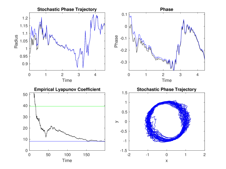
Figure 4: Synchronization of two radial isochron oscillators with common switching noise. We set $\epsilon=0.01$. The radii of the initial conditions differ by $0.1$, and the phases of the initial condition differ by $0.1$. In the top left we plot the radii of the two oscillators, and in the top right we plot the angle (one oscillator is plotted in black, and one in blue). In the bottom right we plot the $x-y$ trajectories of the oscillators: one in black, and one in blue. In the bottom left, we plot $-\epsilon^{-1}t^{-1}\log\big{|}\phi^{1}(t)-\phi^{2}(t)\big{|}$ in black. We plot $\epsilon^{-1}\lambda_{QSS}$ in green, and $\epsilon^{-1}\lambda$ in blue. It can be seen that $\lambda$ is the correct Lyapunov exponent.

Given the deterministic model, the next step is to specify the corresponding PDMP for a single oscillator. One possibility is to assume that one or more of the coefficients switch. For example, in polar coordinates we could take

$$\frac{dr}{dt}=r(\mu_{n}-r_{i}^{2}),\quad\frac{d\phi}{dt}=\eta_{n}-\alpha r^{2}.$$ (5.7)

That is, both the amplitude and angular frequency of each oscillator switch. In Cartesian coordinates we have

$$\frac{dx}{dt} := F_{n,1}({\bf x})=\mu_{n}x-\eta_{n}y-(x^{2}+y^{2})(x-\alpha y)$$

$$\frac{dy}{dt} := F_{n,2}({\bf x})=\mu_{n}y+\eta_{n}x-(x^{2}+y^{2})(y+\alpha x),$$

It immediately follows that the averaged system is given by

$$\frac{dx}{dt} = \overline{F}_{1}({\bf x}):=\overline{\mu}x-\overline{\eta}y-(x^{2}+y^{2})(x-\alpha y)$$

$$\frac{dy}{dt} = \overline{F}_{2}({\bf x}):=\overline{\mu}y+\overline{\eta}x-(x^{2}+y^{2})(y+\alpha x),$$

where

$$\overline{\mu}=\sum_{n\in\Gamma}\mu_{n}\rho_{n},\quad\overline{\eta}=\sum_{n\in\Gamma}\eta_{n}\rho_{n}$$ (5.10)

The corresponding natural frequency is $\overline{\omega}=\overline{\eta}-\alpha\overline{\mu}$. Also note from Eq. (3.1b) that

$$G_{n,1}({\bf x})=(\mu_{n}-\overline{\mu})x-(\eta_{n}-\overline{\eta})y,$$ (5.11a)

$$G_{n,2}({\bf x})=(\mu_{n}-\overline{\mu})y+(\eta_{n}-\overline{\eta})x.$$ (5.11b)

The phase PDMP (4.4) for the radial isochron clock takes the form of a simple velocity jump process

$$\frac{d\theta}{dt} =\omega_{n},$$ (5.12)

since

$${\mathcal{F}}_{n}(\theta) =\sum_{a=1,2}R_{a}(\theta)\left[F_{n,a}(\Phi(\theta))-\overline{F}_{a}(\Phi(\theta))\right]$$

$$=\left[-\sin\theta-\alpha\cos\theta\right]\left[(\mu_{n}-\overline{\mu})\cos\theta-(\eta_{n}-\overline{\eta})\sin\theta\right]$$

$$+\left[\cos\theta-\alpha\sin\theta\right]\left[(\mu_{n}-\overline{\mu})\sin\theta+(\eta_{n}-\overline{\eta})\cos\theta\right]$$

$$=(\eta_{n}-\overline{\eta})-\alpha(\mu_{n}-\overline{\mu})=\omega_{n}-\overline{\omega}.$$ (5.13)

In this case ${\mathcal{F}}_{n}^{\prime}=0$ so Eq. (4.15) implies that the Lyapunov exponents is zero (to leading order in $\epsilon$)– noise-induced synchronization does not occur. This means that one cannot establish that synchronization occurs using the analysis of this paper. Its possible that synchronization might still occur, but the Lyapunov coefficient would be $o(\epsilon)$, and it is not easy to ascertain the synchronization in the numerical results.

A second possibility is to assume that the environments drives the $x$ coordinate with a switching input $I_{n}$ such that $\bar{I}=\sum_{n}\rho_{n}I_{n}=0$. As a concrete example, we take the evolution in Cartesian co-ordinates to be given by

$$\frac{dx}{dt} = \mu x-\eta y-(x^{2}+y^{2})(x-\alpha y)+\frac{x}{\sqrt{x^{2}+y^{2}}}v_{n}^{1}$$

$$\frac{dy}{dt} = \mu y+\eta x-(x^{2}+y^{2})(y+\alpha x)+\frac{y}{\sqrt{x^{2}+y^{2}}}v_{n}^{2}$$

Here $v_{n}=(v^{1}_{k},v^{2}_{k})$ is a jump Markov Process, assuming the following $4$ states

$$v_{1} =(2,-1)\;,\;v_{2}=(-4,-4)$$

$$v_{3} =(-3,2)\;,\;v_{4}=(8.8,7.2),$$

with transition matrix

$$\left(\begin{array}[]{c c c c}0&2&2.5&0.1\\ 1&0&0.5&4\\ 0.5&0.7&0&2\\ 3&0.4&0.25&0\end{array}\right).$$ (5.15)

The state vector and transition matrix were chosen arbitrarily, except for the normalization

$$\sum_{k=1}^{4}\rho_{k}v_{k}=0,$$

to ensure that the averaged system supports a deterministic limit cycle. Hence, the averaged system is given by Eqs. (5.4), whereas the phase PDMP takes the form

$$\frac{d\theta}{dt} =\omega-(\sin\theta+\alpha\cos\theta)v_{n}^{1}+\left[\cos\theta-\alpha\sin\theta\right]v_{n}^{2},$$ (5.16)

In this case ${\mathcal{F}}_{n}^{\prime}\neq 0$ and we expect a pair of hybrid oscillators to synchronize.

Numerical simulations of a pair of radial isochron oscillators evolving according to Eqs. (5.14) with a common environmental drive confirm that synchronization does occur. An example set of results are shown in Fig. 4. Note, in particular, that the quantity

$$-\frac{1}{t}\log\big{|}\phi^{1}(t)-\phi^{2}(t)\big{|}$$

converges to the Lyapunov exponent $\lambda$ given by Eq. (4.15), which was calculated directly from the underlying PDMP, rather than the quasi-steady-state Lyapunov exponent $\lambda_{\rm QSS}$ of Eq. (3.16).

VI Discussion

In this paper we have proved that stable oscillators subject to a common rapidly-switching noise will synchronize , in the vast majority of cases. –Since we gave a counterexample in the previous section, we should probably add this small caveat We have identified the leading order contribution to the Lyapunov exponent, and explained why this is different from the Lyapunov exponent predicted by the quasi-steady-state assumption. These results were shown to be consistent with a simulation of the radial isochron oscillator subject to a common environmental noise.

In more detail, we have seen that the phases of rapidly-switching oscillators converge at a rate of $\exp\big{(}-\epsilon\lambda t\big{)}$, where $\epsilon$ is the timescale of the switching. Thus in the limit as the switching gets faster and faster (i.e. $\epsilon\to 0$), the rate of synchronization gets slower and slower. This is not surprising, since we know that in the deterministic $\epsilon=0$ limit, the oscillators will in general never synchronize if their starting conditions are different. These results are contingent on the two oscillators staying in the attracting neighborhood of the limit cycle. Indeed we have shown in Maclaurin18b that the timescale over which the oscillators remain close to the limit cycle scales as $\exp\big{(}c\epsilon^{-1}\big{)}$, for a constant $c$. In fact if one were to continue the analysis of this paper, and develop precise error bounds for the probability of the two oscillators synchronizing, then one would find that the smaller $\epsilon$ is, then the more likely it is that the oscillators, once they are almost synchronized, stay almost synchronized. In summary: as $\epsilon\to 0$, the oscillators synchronize at a slower and slower rate, but stay synchronized with a higher and higher probability.

Appendix A

The basic steps of the QSS reduction of the population equations (3.3) are as follows:

a) Decompose the probability density as

$$p_{n}({\bf x},t)=C({\bf x},t)\rho_{n}+\epsilon w_{n}({\bf x},t),$$

where $\sum_{n}p_{n}({\bf x},t)=C({\bf x},t)$ and $\sum_{n}w_{n}({\bf x},t)=0$. Substituting into Eq. (2.6) yields

$$\rho_{n}\frac{\partial C}{\partial t}+\epsilon\frac{\partial w_{n}}{\partial t} = -\sum_{i=1}^{M}\nabla_{i}\cdot\left(F_{n}(x_{i})[\rho_{n}C+\epsilon w_{n}]\right)$$

$$\quad+\frac{1}{\epsilon}\sum_{m\in\Gamma}A_{nm}[\rho_{m}C+\epsilon w_{m}]$$

Summing both sides with respect to $n$ then gives

$$\frac{\partial C}{\partial t}=-\sum_{i=1}^{M}\left\{\nabla_{i}\cdot\left[\overline{F}(x_{i})C\right]+\epsilon\sum_{n\in\Gamma}\nabla_{i}\cdot\left[F_{n}(x_{i})w_{n}\right].\right\}$$ (A.1)

b) Using the equation for $C$ and the fact that ${\bf A}\rho=0$, we have

$$\epsilon\frac{\partial w_{n}}{\partial t}=\sum_{m\in\Gamma}A_{nm}w_{m}$$

$$-\rho_{n}\sum_{i=1}^{M}\left\{\nabla_{i}\cdot\left[F_{n}(x_{i})C\right]-\nabla_{i}\cdot\left[\overline{F}(x_{i})C\right]\right\}$$

$$-\epsilon\sum_{i=1}^{M}\left\{\left[\nabla_{i}\cdot\left(F_{n}(x_{i})\omega_{n}\right)-\rho_{n}\sum_{m\in\Gamma}\nabla_{i}\cdot\left[F_{m}(x_{i})w_{m}\right]\right]\right\}.$$

c) Introduce the asymptotic expansion

$$w_{n}\sim{w}_{n}^{(0)}+\epsilon{w}_{n}^{(1)}+\epsilon^{2}{w}_{n}^{(2)}+\ldots$$

and collect $O(1)$ terms:

$$\sum_{m\in\Gamma}A_{nm}w^{(0)}_{m}=\rho_{n}\sum_{i=1}^{M}\nabla_{i}\cdot\left[F_{n}(x_{i})-\overline{F}(x_{i})]C\right].$$

The Fredholm alternative theorem show that this has a solution, which is unique on imposing the condition $\sum_{n}w^{(0)}_{n}({\bf x},t)=0$:

$$w^{(0)}_{n}({\bf x})=\sum_{m\in\Gamma}A^{\dagger}_{nm}\rho_{m}\sum_{j=1}^{N}\left(\nabla_{j}\cdot\left[F_{m}(x_{j})-\overline{F}(x_{j})]C\right]\right).$$

where ${\bf A}^{\dagger}$ is the pesudo-inverse of the generator ${\bf A}$.

d) Combining Eqs. (Appendix A) and (A.1) shows that $C$ evolves according to the Fokker-Planck (FP) equation

$$\frac{\partial C}{\partial t} = -\sum_{i=1}^{M}\nabla_{i}\cdot\left[\overline{F}(x_{i})C\right]-\epsilon\sum_{i,j=1}^{M}\sum_{n,m\in\Gamma}A_{nm}^{\dagger}\rho_{m}$$

$$\times\nabla_{i}\cdot\left(F_{n}(x_{i})\nabla_{j}\cdot\left[F_{m}(x_{j})-\overline{F}(x_{j})]C\right]\right).$$

Using the fact that $\sum_{m}w_{n}=0$, this can be rewritten in the Stratonovich form (3.1a). One typically has to determine the pseudo-inverse of ${\bf A}$ numerically.

Appendix B

In this appendix we show that the $O(\Delta t_{k})$ term in Eq. (IV.2) does not contribute to the Lyapunov exponent in the long time limit. First, recall that

$$\psi(t_{l})^{-1}[{\mathcal{H}}_{n_{l}}(x_{1})-{\mathcal{H}}_{n_{l}}(x_{2})]\simeq\mathcal{F}^{\prime}_{n_{l}}(\phi).$$

From now on, we drop the dependence of $\mathcal{F}$ on $\phi$ to simplify notation. We start by understanding the leading order second moment of $\mathcal{M}$ terms, i.e.

$$V_{\mathcal{M}}:=\mathbb{E}\bigg{[}\bigg{(}\sum_{l=k}^{l=k+\mathcal{M}}\mathcal{F}^{\prime}_{n_{l}}\Delta t_{l}\bigg{)}^{2}\bigg{]}.$$

(An important reason that we do this is that, as noted in Sect. IV.C, the rate of change of this term with respect to time yields the Lyapunov exponent of the quasi-steady-state reduction.) $\mathcal{M}$ will be taken to be large enough that the system has switched sufficiently many times for the quasi-steady-state approximation to be accurate, but $\mathcal{M}$ is also taken to be sufficiently small that $x_{1},x_{2}$ and $\phi$ are approximately constant. In other words, $1\ll\mathcal{M}\ll\epsilon^{-1}$. To this end, we expand out the square to obtain

$$\mathbb{E}\bigg{[}\bigg{(}\sum_{l=k}^{l=k+\mathcal{M}}\mathcal{F}^{\prime}_{n_{l}}\Delta t_{l}\bigg{)}^{2}\bigg{]}\\ =\sum_{l=k}^{l=k+\mathcal{M}}\sum_{j=k}^{j=k+\mathcal{M}}\mathbb{E}\bigg{[}\Delta t_{l}\Delta t_{j}\mathcal{F}^{\prime}_{n_{l}}\mathcal{F}^{\prime}_{n_{j}}\bigg{]}\\ \simeq 2\sum_{l=k}^{l=k+\mathcal{M}}\sum_{j=0}^{\mathcal{M}}\mathbb{E}\bigg{[}\Delta t_{l}\Delta t_{l+j}\mathcal{F}^{\prime}_{n_{l}}\mathcal{F}^{\prime}_{n_{j+l}}\bigg{]}.$$

The reason why the above approximation is very accurate is that the number of extra terms obtained through the reindexing is negligible compared to the total number of terms.

Now we can approximate the above equation by using the fact that the correlations between $\Delta t_{l}\mathcal{F}^{\prime}_{n_{l}}$ and $\Delta t_{l+j}\mathcal{F}_{n_{l+j}}^{\prime}$ decay exponentially fast in $j$, thanks to the Perron-Frobenius Theorem. Since, as demonstrated in Sect. IV, the mean of $\Delta t_{l+j}\Delta F_{n_{l+j}}$ is $0$, the contribution of the terms with asymptotically large $j$ will be negligible. We now explain these statements in more detail.

Let $P=(P_{km})$ be the matrix with elements $P_{km}=\lambda_{m}^{-1}W_{km}$. If one knows that the system was in state $m$, and that it has jumped, then it jumps to state $k$ with probability $P_{km}$. The Perron-Frobenius Theorem implies that

$$\lim_{q\to\infty}P^{q}=B,$$ (B.1)

where $B$ is the rank-$1$ matrix with the $i^{th}$ element of each column equal to $\frac{1}{\sum_{a\in\Gamma}\rho_{a}\lambda_{a}}\lambda_{i}\rho_{i}$. Furthermore the convergence is exponentially fast, i.e.

$$||P^{q}-B||=O\big{(}\exp(-q)\big{)},$$ (B.2)

for any matrix norm saloff1997lectures .

Now

$$2\sum_{l=k}^{l=k+\mathcal{M}}\sum_{j=0}^{\mathcal{M}}\mathbb{E}\bigg{[}\Delta t_{l}\Delta t_{l+j}\mathcal{F}^{\prime}_{n_{l}}\mathcal{F}^{\prime}_{n_{j+l}}\bigg{]}=\\ 2\sum_{l=k}^{l=k+\mathcal{M}}\sum_{p,m\in\Gamma}\mathbb{P}\big{(}n_{l}=m\big{)}\mathbb{E}\big{[}\Delta t_{l}\mathcal{F}^{\prime}_{n_{l}}|n_{l}=m\big{]}\\ \times\sum_{j=0}^{\infty}\big{(}P^{j}\big{)}_{pm}\mathbb{E}\big{[}\Delta t_{l+j}\mathcal{F}^{\prime}_{n_{j+l}}|n_{j+l}=p\big{]}\\ \simeq 2\epsilon^{2}\sum_{l=k}^{l=k+\mathcal{M}}\sum_{p,m\in\Gamma}\frac{\mathcal{F}^{\prime}_{p}\mathcal{F}^{\prime}_{m}}{\lambda_{m}\lambda_{p}}\mathbb{P}\big{(}n_{l}=m\big{)}\sum_{j=0}^{\mathcal{M}}\big{(}P^{j}\big{)}_{pm}.$$

since, because $x_{1},x_{2}$ change by a negligible amount over this timescale (as $\mathcal{M}=o(\epsilon^{-1})$), if $n_{i}=n_{j}$, then $\mathcal{F}^{\prime}_{n_{i}}\simeq\mathcal{F}^{\prime}_{n_{j}}$.

If we substitute $P^{j}$ for its limit $B$ in the above, we obtain

$$\frac{1}{\sum_{a\in\Gamma}\rho_{a}\lambda_{a}}\sum_{j=0}^{\mathcal{M}}\sum_{l=k}^{l=k+\mathcal{M}}\sum_{p,m\in\Gamma}\frac{\mathcal{F}^{\prime}_{m}\mathcal{F}^{\prime}_{p}}{\lambda_{m}\lambda_{p}}\mathbb{P}\big{(}n_{l}=m\big{)}\rho_{p}\lambda_{p}=0,$$

since $\sum_{p\in\Gamma}\rho_{p}\Delta\mathcal{F}^{\prime}_{p}=0$. This is what we expect in light of the above discussion, because the system decorrelates after infinitely many jumps, and the mean is zero.

In light of (B.2), the above discussion means that for large $\mathcal{M}$ we can extend the summation to $\infty$, without much of a loss of accuracy

$$2\sum_{l=k}^{l=k+\mathcal{M}}\sum_{j=0}^{\mathcal{M}}\mathbb{E}\bigg{[}\Delta t_{l}\Delta t_{l+j}\mathcal{F}^{\prime}_{n_{l}}\mathcal{F}^{\prime}_{n_{j+l}}\bigg{]}\\ \simeq 2\epsilon^{2}\sum_{l=k}^{l=k+\mathcal{M}}\sum_{p,m\in\Gamma}\frac{\mathcal{F}^{\prime}_{p}\mathcal{F}^{\prime}_{m}}{\lambda_{m}\lambda_{p}}\mathbb{P}\big{(}n_{l}=m\big{)}\sum_{j=0}^{\infty}\big{(}P^{j}\big{)}_{pm}\\ \simeq\frac{2\epsilon^{2}\mathcal{M}}{\sum_{a\in\Gamma}\rho_{a}\lambda_{a}}\sum_{p,m\in\Gamma}\frac{\rho_{m}\mathcal{F}^{\prime}_{p}\mathcal{F}^{\prime}_{m}}{\lambda_{p}}\sum_{j=0}^{\infty}\big{(}P^{j}\big{)}_{pm},$$ (B.3)

since, as explained above, the number of jumps to state $m$ is approximately $\mathcal{M}\rho_{m}\lambda_{m}/\big{(}\sum_{a\in\Gamma}\rho_{a}\lambda_{a}\big{)}$.

Now we wish to understand how the above term relates to the pseudo-inverse of $A$ (which occurred in the QSS SDE of Appendix A). In fact we claim that

$$-\sum_{j=0}^{\infty}\sum_{p,q\in\Gamma}A_{mp}\lambda_{p}^{-1}\big{(}P^{j}\big{)}_{pq}\rho_{q}\mathcal{F}^{\prime}_{q}=\rho_{m}\mathcal{F}^{\prime}_{m},$$ (B.4)

which will allow us to establish the identity in (B.5).

Note that the summation on the left converges because $\sum_{p\in\Gamma}A_{mp}\lambda_{p}^{-1}B_{pq}=0$ for every $q,m\in\Gamma$, and therefore the convergence is exponential in $j$ thanks to (B.2). We expand out the left hand side, substituting $A$ and using a truncated summation, i.e. for some $R\in\mathbb{Z}^{+}$,

$$-\sum_{j=0}^{R}\sum_{p,q\in\Gamma}A_{mp}\lambda_{p}^{-1}\big{(}P^{j}\big{)}_{pq}\mathcal{F}^{\prime}_{q}\rho_{q}$$

$$=-\sum_{j=0}^{R}\sum_{p,q\in\Gamma}\big{(}W_{mp}-\lambda_{p}\delta(m,p)\big{)}\lambda_{p}^{-1}\big{(}P^{j}\big{)}_{pq}\mathcal{F}^{\prime}_{q}\rho_{q}$$

$$=\sum_{q\in\Gamma}\bigg{\{}\sum_{j=0}^{R}\big{(}P^{j}\big{)}_{mq}\mathcal{F}_{q}^{\prime}\rho_{q}-\sum_{j=1}^{R+1}\big{(}P^{j}\big{)}_{mq}\mathcal{F}^{\prime}_{q}\rho_{q}\bigg{\}}$$

$$=\mathcal{F}^{\prime}_{m}\rho_{m}-\sum_{q\in\Gamma}\big{(}P^{R+1}\big{)}_{mq}\mathcal{F}^{\prime}_{q}\rho_{q}.$$

Now $\sum_{q\in\Gamma}B_{mq}\mathcal{F}^{\prime}_{q}\rho_{q}=0$, because, as noted just below (B.1), the columns of $B$ are all the same, and $\sum_{q\in\Gamma}\mathcal{H}_{q}\rho_{q}=0$. Since $P^{R+1}\to B$ as $R\to\infty$, when we take $R\to\infty$, we obtain (B.4).

It follows from (B.4) that

$$\sum_{j=0}^{\infty}\sum_{q\in\Gamma}\lambda_{p}^{-1}\big{(}P^{j}\big{)}_{pq}\rho_{q}\mathcal{F}^{\prime}_{q}=-A^{\dagger}_{pm}\rho_{m}\mathcal{F}^{\prime}_{m},$$ (B.5)

where we recall the pseudo-inverse $A^{\dagger}$, defined in the previous section on the QSS approximation.

Substituting this identity into (B.3), we find that

$$\sum_{l=k}^{l=k+\mathcal{M}}\sum_{j=0}^{\mathcal{M}}\mathbb{E}\bigg{[}\Delta t_{l}\Delta t_{l+j}\mathcal{F}^{\prime}_{n_{l}}\mathcal{F}^{\prime}_{j+l}\bigg{]}\\ \simeq-\frac{\epsilon^{2}\mathcal{M}}{\sum_{a\in\Gamma}\rho_{a}\lambda_{a}}\sum_{p,q\in\Gamma}\mathcal{A}^{\dagger}_{pq}\mathcal{F}^{\prime}_{p}\mathcal{F}^{\prime}_{q}\rho_{q}.$$ (B.6)

This implies that

$$\frac{1}{2(t_{k+\mathcal{M}}-t_{k})}\mathcal{V}_{M}\simeq-\epsilon\sum_{p,q\in\Gamma}\mathcal{A}^{\dagger}_{pq}\mathcal{F}^{\prime}_{p}\mathcal{F}^{\prime}_{q}\rho_{q},$$ (B.7)

using the expression for $\tau_{\mathcal{M}}=t_{k+\mathcal{M}}-t_{k}$ in (4.11). Just like the end of Sect. IV.B, we find that

$$\frac{1}{2t_{K}}\mathbb{E}\bigg{[}\bigg{(}\sum_{l=0}^{K}\mathcal{F}^{\prime}_{l}\Delta t_{l}\bigg{)}^{2}\bigg{]}$$

$$\qquad\simeq-\frac{\epsilon}{2\pi}\int_{0}^{2\pi}\sum_{p,q\in\Gamma}\mathcal{A}^{\dagger}_{pq}\mathcal{F}^{\prime}_{p}(\theta)\mathcal{F}^{\prime}_{q}(\theta)\rho_{q}d\theta.$$

$$\qquad=\lambda_{QSS}$$ (B.8)

We have thus established the claim in (4.16).

The final step in the proof is to show that

$$\mathbb{P}\bigg{(}t_{q\mathcal{M}}^{-1}\sum_{l=0}^{q\mathcal{M}}\mathcal{F}^{\prime}_{n_{l}}\Delta t_{l}\geq O(\epsilon)\bigg{)}\ll 1.$$ (B.9)

(Technically, this probability is conditional on both systems staying in a neighborhood of the limit cycle until the time $t_{q\mathcal{M}}$. We have demonstrated that this occurs for very long times, with very high probability, elsewhere Maclaurin18b .) To this end, we use Chebyshev’s Inequality, noting that

$$\mathbb{P}\bigg{(}t_{q\mathcal{M}}^{-1}\sum_{l=0}^{q\mathcal{M}}\mathcal{F}^{\prime}_{n_{l}}\Delta t_{l}\geq a\bigg{)}\\ \leq\frac{1}{(at_{q\mathcal{M}})^{2}}\mathbb{E}\bigg{[}\bigg{(}\sum_{l=0}^{q\mathcal{M}}\mathcal{F}^{\prime}_{n_{l}}\Delta t_{l}\bigg{)}^{2}\bigg{]}.$$ (B.10)

We now bound the rate of growth in time of the expectation on the right. The immediate use of this bound will be to show that the probability is negligible. A secondary use is that it will help us understand how this discrete approximation compares to the QSS SDE.

We must thus understand the second order moment of $q\mathcal{M}$ terms, ie.

$$\mathbb{E}\bigg{[}\bigg{(}\sum_{l=0}^{q\mathcal{M}}\mathcal{F}^{\prime}_{n_{l}}\Delta t_{l}\bigg{)}^{2}\bigg{]}=\sum_{l=0}^{q\mathcal{M}}\sum_{j=0}^{q\mathcal{M}}\mathbb{E}\bigg{[}\Delta t_{l}\Delta t_{j}\mathcal{F}^{\prime}_{n_{l}}\mathcal{F}^{\prime}_{n_{j}}\bigg{]}$$

$$\quad\simeq 2\sum_{l=0}^{q\mathcal{M}}\sum_{j=0}^{q\mathcal{M}}\mathbb{E}\bigg{[}\Delta t_{l}\Delta t_{l+j}\mathcal{F}^{\prime}_{n_{l}}\mathcal{F}^{\prime}_{n_{j+l}}\bigg{]}$$

$$\quad=2\sum_{r=1}^{q}\sum_{l=(r-1)\mathcal{M}}^{l=r\mathcal{M}}\sum_{j=0}^{q\mathcal{M}}\mathbb{E}\bigg{[}\Delta t_{l}\Delta t_{l+j}\mathcal{F}^{\prime}_{n_{l}}\mathcal{F}^{\prime}_{n_{j+l}}\bigg{]}.$$

Using the estimate derived in (B.6), we find that

$$\mathbb{E}\bigg{[}\bigg{(}\sum_{l=0}^{q\mathcal{M}}\mathcal{F}^{\prime}_{n_{l}}\Delta t_{l}\bigg{)}^{2}\bigg{]}-\mathbb{E}\bigg{[}\bigg{(}\sum_{l=0}^{(q-1)\mathcal{M}}\mathcal{F}^{\prime}_{n_{l}}\Delta t_{l}\bigg{)}^{2}\bigg{]}\simeq-\frac{2\epsilon^{2}\mathcal{M}}{\sum_{a\in\Gamma}\rho_{a}\lambda_{a}}\sum_{p,u\in\Gamma}{\mathcal{A}}_{pu}^{\dagger}\mathcal{F}^{\prime}_{p}\mathcal{F}^{\prime}_{u}\rho_{u}.$$

Hence, using the expression for the time for $\mathcal{M}$ jumps in (4.11),

$$\frac{1}{\sum_{l=(q-1)\mathcal{M}+1}^{q\mathcal{M}}\Delta t_{l}}\left\{\mathbb{E}\bigg{[}\bigg{(}\sum_{l=0}^{q\mathcal{M}}\mathcal{F}^{\prime}_{n_{l}}\Delta t_{l}\bigg{)}^{2}\bigg{]}-\mathbb{E}\bigg{[}\bigg{(}\sum_{l=0}^{(q-1)\mathcal{M}}\mathcal{F}^{\prime}_{n_{l}}\Delta t_{l}\bigg{)}^{2}\bigg{]}\right\} \simeq-\frac{\sum_{n\in\Gamma}\rho_{n}\lambda_{n}}{\epsilon\mathcal{M}}\frac{2\epsilon^{2}\mathcal{M}}{\sum_{a\in\Gamma}\rho_{a}\lambda_{a}}\sum_{p,u\in\Gamma}{\mathcal{A}}_{pu}^{\dagger}\mathcal{F}^{\prime}_{p}\mathcal{F}^{\prime}_{u}\rho_{u}$$

$$=-2\epsilon\sum_{p,u\in\Gamma}{\mathcal{A}}_{pu}^{\dagger}\mathcal{F}^{\prime}_{p}\mathcal{F}^{\prime}_{u}\rho_{u}.$$

Since the above expression approximates the derivative with respect to time, after re-integrating we find that

$$\mathbb{E}\bigg{[}\bigg{(}\sum_{l=0}^{q\mathcal{M}}\mathcal{F}^{\prime}_{l}\Delta t_{l}\bigg{)}^{2}\bigg{]}\simeq-2\epsilon\int_{0}^{t_{q\mathcal{M}}}\sum_{p,u\in\Gamma}{\mathcal{A}}^{\dagger}_{pu}\mathcal{F}^{\prime}_{p}(\theta_{s})\mathcal{F}^{\prime}_{u}(\theta_{s})\rho_{u}ds.$$ (B.11)

It then follows from the above expression and (B.10) that

$$\mathbb{P}\bigg{(}t_{q\mathcal{M}}^{-1}\sum_{l=0}^{q\mathcal{M}}\mathcal{F}^{\prime}_{n_{l}}\Delta t_{l}\geq a\bigg{)}=O\bigg{(}\frac{\epsilon}{a^{2}t_{q\mathcal{M}}}\bigg{)}.$$ (B.12)

This clearly goes to zero as $q\to\infty$. We have thus justified why the linear terms in $\Delta t_{l}$ in (IV.2) are $o(\epsilon)$ over long periods of time, and this implies (4.14). This is why the quadratic terms in $\Delta t_{l}$ dominate the linear ones over long periods of time.

References

- [1] A. Winfree, The geometry of biological time, Springer-Verlag, New York (1980).
- [2] Y. Kuramoto, Chemical Oscillations, Waves and Turbulence, Springer-Verlag, New-York (1984).
- [3] G. B. Ermentrout and N. Kopell, Frequency plateaus in a chain of weakly coupled oscillators, I., SIAM J. Math. Anal. 15 215-237 (1984).
- [4] L. Glass and M. C. Mackey, From Clocks to Chaos, Princeton Univ Press, Princeton (1988).
- [5] G. B. Ermentrout and N. Kopell, Multiple pulse interactions and averaging in systems of coupled neural oscillators, J. Math. Biol. 29 195-217 (1991).
- [6] G. B. Ermentrout, Type I membranes, phase resetting curves, and synchrony, Neural Comput. 8 979 (1986)
- [7] E. Brown, J. Moehlis, and P. Holmes, On the phase reduction and response dynamics of neural oscillator populations., Neural Comput., 16 673–715 (2004).
- [8] P. Ashwin, S. Coombes and R. Nicks, Mathematical frameworks for oscillatory network dynamics in neuroscience, J. Math. Neurosci., 6 (2016).
- [9] H. Nakao, Phase reduction approach to synchronization of nonlinear oscillators.Contemporary Physics 57 188-214 (2016)
- [10] J. N. Teramae and D. Tanaka, Robustness of the noise-induced phase synchronization in a general class of limit cycle oscillators, Phys. Rev. Lett., 93 204103 (2004)
- [11] D. S. Goldobin and A. Pikovsky, Synchronization and desynchronization of self–sustained oscillators by common noise, Phys. Rev. E, 71 045201 (2005).
- [12] H. Nakao, K. Arai, and Y. Kawamura, Noise-induced synchronization and clustering in ensembles of uncoupled limit cycle oscillators, Phys. Rev. Lett., 98 184101 (2007)
- [13] K. Yoshimura and K. Arai, Phase reduction of stochastic limit cycle oscillators, Phys. Rev. Lett. 101 154101 (2008).
- [14] J. N. Teramae, H. Nakao, and G. B. Ermentrout, Stochastic phase reduction for a general class of noisy limit cycle oscillators, Phys. Rev. Lett. 102 194102 (2009).
- [15] C. Ly and G. B. Ermentrout, Synchronization of two coupled neural oscillators receiving shared and unshared noisy stimuli. J. Comput. Neurosci. 26 425-443 (2009).
- [16] G. B. Ermentrout, Noisy oscillators, in Stochastic methods in neuroscience, C R Laing and G J Lord, eds., Oxford University Press, Oxford, 2009.
- [17] R. F. Galan, G. B. Ermentrout and N. N. Urban, Optimal time scale for spike-time reliability: theory, simulations and experiments J. Neurophysiol. 99 277-283 (2008).
- [18] T. Zhou, J. Zhang, Z. Yuan and L. Chen, Synchronization of genetic oscillators. Chaos 18 037126 (2008).
- [19] L. Potvin-Trottier, N. D Lord, G. Vinnicombe and J. Paulsson Synchronous long-term oscillations in a synthetic gene circuit Nature 538 514-517 (2016).
- [20] Z. F. Mainen and T. J. Sejnowski, Reliability of spike timing in neocortical neurons, Science 268 1503 (1995).
- [21] R. F. Galan, N. Fourcaud-Trocme, G. B. Ermentrout and N. N. Urban, Correlation-induced synchronization of oscillations in olfactory bulb neurons. Journal of Neuroscience 26 3646 (2006).
- [22] A. Uchida, R. McAllister, and R. Roy, Consistency of Nonlinear System Response to Complex Drive Signals Phys. Rev. Lett. 93 244102 (2004).
- [23] B. T. Grenfell, K. Wilson, B. F. Finkenstadt, T. N. Coulson, S. Murray, S. D. Albon, J. M. Pemberton, T. H. Clutton-Brock, and M. J. Crawley, Noise and determinism in synchronized sheep dynamics, Nature 394, 674 (1998).
- [24] H. Nakao, K. Arai, K. Nagai, Y. Tsubo, and Y. Kuramoto, Synchrony of limit-cycle oscillators induced by random external impulses, Phys. Rev. E 72 026220 (2005).
- [25] K. Nagai, H. Nakao, and Y. Tsubo, Synchrony of neural oscillators induced by random telegraphic currents. Phys. Rev. E 71 036217 (2005).
- [26] D. S. Goldobin, J. Teramae, H. Nakao, and G. B. Ermentrout, Dynamics of limit-cycle oscillators subject to general noise, Phys. Rev. Lett. 105 154101 (2010).
- [27] I. Bena. Dichotomous Markov noise: exact results for out-of-equilibrium systems. Int. J. Mod. Phys. B 20 2825 (2006).
- [28] M. H. A. Davis, Piecewise-deterministic Markov processes: A general class of non-diffusion stochastic models. Journal of the Royal Society, Series B (Methodological) 46 353-388 (1984).
- [29] P. C. Bressloff. Stochastic switching in biology: from genotype to phenotype (Topical Review) J. Phys. A 50 133001 (2017)
- [30] T. B. Kepler and T. C. Elston, Stochasticity in transcriptional regulation: origins, consequences, and mathematical representations Biophys. J. 81 3116-3136 (2001)
- [31] R. Karmakar and I. Bose,Graded and binary responses in stochastic gene expression, Phys. Biol. 1197-204 (2004).
- [32] S. Zeiser, U. Franz, O. Wittich and V. Liebscher, Simulation of genetic networks modelled by piecewise deterministic Markov processes IET Syst. Biol. 2 113-135 (2008)
- [33] M. W. Smiley and S. R. Proulx, Gene expression dynamics in randomly varying environments. J. Math. Biol. 61, 231-251 (2010).
- [34] A. Hilfinger and J. Paulsson Separating intrinsic from extrinsic fluctuations in dynamic biological systems Proceedings of the National Academy of Sciences. 108 (2011)
- [35] J. M. Newby, Isolating intrinsic noise sources in a stochastic genetic switch, Phys. Biol. 9 026002 (2012)
- [36] A. Singh A. Singh and M. Soltani Quantifying Intrinsic and Extrinsic Variability in Stochastic Gene Expression Models PLOS One 8 e84301 (2013).
- [37] C. Zechner and H. Koeppl Uncoupled Analysis of Stochastic Reaction Networks in Fluctuating Environments PLoS Comp Biology. 10 e100394 (2014).
- [38] J. M. Newby, Bistable switching asymptotics for the self regulating gene, J. Phys. A 48 185001 (2015).
- [39] P. G. Hufton, Y. T. Lin, T. Galla and A. J. McKane, Intrinsic noise in systems with switching environments Phys. Rev. E 93 052119 (2016).
- [40] P. C. Bressloff and E. Levien Robustness of stochastic chemical reaction networks to extrinsic noise: the role of deficiency Multiscale Modeling and Simulation. In press (2018).
- [41] J. M. Newby and P. C. Bressloff Quasi-steady state reduction of molecular-based models of directed intermittent search. Bull Math Biol 72 1840-1866 (2010)
- [42] C. W. Gardiner, Handbook of stochastic methods, 4th edition, Springer, Berlin (2009).
- [43] A. Faggionato, D. Gabrielli and M. R. Crivellari. Averaging and large deviation principles for fully-coupled piecewise deterministic Markov processes and applications to molecular motors. Markov Processes and Related Fields 16 497-548 (2010).
- [44] D. Gonze, J. Halloy and P. Gaspard, Biochemical clocks and molecular noise: theoretical study of robustness factors., J. Chem. Phys., 116 10997–11010 (2002).
- [45] H. Koeppl, M. Hafner, A. Ganguly and A. Mehrotra, Deterministic characterization of phase noise in biomolecular oscillators., Phys. Biol. 8 055008 (2011)
- [46] M. Bonnin, Amplitude and phase dynamics of noisy oscillators, Int. J. Circuit Th. Appl., 45 636–659 (2017).
- [47] P. C. Bressloff and J. N. Maclaurin. Variational method for analyzing stochastic limit cycle oscillators. SIAM J. Appl. Dyn. Syst. 17 2205-2233 (2018).
- [48] G. Giacomin, C. Poquet and A. Shapira, Small noise and long time phase diffusion in stochastic limit cycle oscillators J. Diff. Eqns. 264 1019-1049 (2018).
- [49] P. C. Bressloff and J. N. Maclaurin. Variational method for analyzing stochastic hybrid oscillators. Chaos. 28 063105 (2018).
- [50] L. Saloff-Coste, Lectures on finite markov chains, in Lectures on probability theory and statistics, Springer pp. 301–413 (1997).