Magnus-type Integrator for the Finite Element Discretization of Semilinear Parabolic non-Autonomous SPDEs Driven by multiplicative noise

Abstract

This paper aims to investigate numerical approximation of a general second order non-autonomous semilinear parabolic stochastic partial differential equation (SPDE) driven by multiplicative noise. Numerical approximations of autonomous SPDEs are thoroughly investigated in the literature, while the non-autonomous case is not yet understood. We discretize the non-autonomous SPDE driven by multiplicative noise by the finite element method in space and the Magnus-type integrator in time. We provide a strong convergence proof of the fully discrete scheme toward the mild solution in the root-mean-square $L^{2}$ norm. The result reveals how the convergence orders in both space and time depend on the regularity of the noise and the initial data. In particular, for multiplicative trace class noise we achieve convergence order $\mathcal{O}\left(h^{2}\left(1+\max(0,\ln\left(t_{m}/h^{2}\right)\right)+\Delta t^{1/2}\right)$. Numerical simulations to illustrate our theoretical finding are provided.

1 Introduction

We consider the numerical approximations of the following semilinear parabolic non-autonomous SPDE driven by mutiplicative noise

$$\left\{\begin{array}[]{ll}dX=[A(t)X+F(t,X)]dt+B(t,X)dW(t),\quad\text{in}\quad\Lambda\times(0,T],\\ X(0)=X_{0},\quad\hskip 139.41832pt\text{in}\quad\Lambda,\end{array}\right.$$ (3)

in the Hilbert space $L^{2}(\Lambda)$, where $\Lambda$ is a bounded domain of $\mathbb{R}^{d}$, $d=1,2,3$ and $T\in(0,\infty)$. The family of unbounded linear operators $A(t)$ are not necessarily self-adjoint. Each $A(t)$ is assumed to generate an analytic semigroup $S_{t}(s):=e^{A(t)s}$. The nonlinear functions $F$ and $B$ are respectively the drift and the diffusion parts. Precise assumptions on $A(t)$, $F$ and $B$ to ensure the existence of the unique mild solution of (3) are given in the next section. The random initial data is denoted by $X_{0}$. We denote by $(\Omega,\mathcal{F},\mathbb{P})$ a probability space with a filtration $(\mathcal{F}_{t})_{t\in[0,T]}\subset\mathcal{F}$ that fulfills the usual conditions (see [30, Definition 2.1.11]). The noise term $W(t)$ is assumed to be a $Q$-Wiener process defined on a filtered probability space $\left(\Omega,\mathcal{F},\mathbb{P},\{\mathcal{F}_{t}\}_{t\in[0,T]}\right)$, where the covariance operator $Q:H\longrightarrow H$ is assumed to be linear, self adjoint and positive definite. It is well known [30] that the noise can be represented as

$$W(t,x)=\sum_{i=0}^{\infty}\sqrt{q}_{i}e_{i}(x)\beta_{i}(t),$$ (4)

where $(q_{i},e_{i})_{i\in\mathbb{N}}$ are the eigenvalues and eigenfunctions of the covariance operator $Q$, and $(\beta_{i})_{i\in\mathbb{N}}$ are independent and identically distributed standard Brownian motions. The deterministic counterpart of (3) finds applications in many fields such as quantum fields theory, electromagnetism, nuclear physics (see e.g. [4] and references therein). It is worth to mention that models based on SPDEs can offer a more realistic representation of the system than models based only on PDEs, due to uncertainty in the input data. In many situations it is very hard to exhibit explicit solutions of SPDEs. For instance the following non-autonomous linear Stratonovich stochastic ordinary differential equation

$$dy=G_{0}(t)ydt+\sum_{j=1}^{d}G_{j}(t)ydW_{j}(t),\quad y(0)=y_{0}\in\mathbb{R}^{m}$$ (5)

does not have explicit solution (see e.g. [2, 18]), unless $G_{i}$ and $G_{j}$ commute for all $i,j\geq 0$. Numerical algorithms are therefore excellent tools to provide good approximations. Numerical approximations of (3) based on implicit, explicit Euler methods and exponential integrators with $A(t)=A$, where $A$ is self-adjoint are thoroughly investigated in the literature, see e.g. [16, 19, 20, 37, 38, 23, 36] and the references therein. If we turn our attention to the case of time independent operator $A(t)=A$, with $A$ not necessary self-adjoint, the list of references become remarkably short, see e.g., [22, 26]. To the best of our knowledge numerical approximations of (3) with time dependent linear operator $A(t)$ are not yet investigated in the scientific literature, due to the complexity of the linear operator $A(t)$ and its semigroup $S_{t}(s):=e^{A(t)s}$. Our aim in this paper is to fill that gap and propose an explicit numerical scheme to approximate (3). We use the finite element method for spatial discretization and Magnus-type integrator for temporal discretization. Magnus-type integrator is based on a truncation of Magnus expansion, which was first proposed in [25] to represent the solution of non-autonomous homogeneous differential equation in the exponential form. Magnus expansion was further studied in [2, 3, 4]. The first numerical method based on magnus expansion was proposed in [14] for deterministic time-dependent homogeneous Schröndinger equation. The study in [14] was extended in [10] for partial differential equation of the following form

$$u^{\prime}(t)=A(t)u(t)+b(t),\quad 0<t\leq T,\quad u(0)=u_{0}.$$ (6)

We follow [10] and apply the Magnus-type integrator method to the semi-discrete problem (43) and obtain the fully discrete scheme (47), called stochastic Magnus-type integrators (SMTI). We investigate the strong convergence of the new fully discrete scheme toward the exact solution. Due to the complexity of the linear operator and the corresponding semi discrete linear operator after space discretisation, novel technical estimates are provided to achieve convergence orders comparable of that of autonomous SPDEs [22, 19, 26]. The result indicates how the convergence orders in both space and time depend on the regularity of the initial data and the noise. In particular for multiplicative trace class noise, we achieve optimal convergence orders of $\mathcal{O}\left(h^{\beta}+\Delta t^{\min(\beta,1)/2}\right)$, where $\beta$ is the regularity’s parameter, defined in Assumption 1.

The rest of this paper is organised as follows. Section 2 provides the general setting, the fully discrete scheme and the main result. In Section 3 we provide some preparatory results and we present the proof of the main result. Section 4 provides some numerical experiments to confirm our theoretical result.

2 Mathematical setting, numerical scheme and main result

2.1 Notations and main assumptions

Let $(H,\langle.,.\rangle_{H},\|.\|)$ be a separable Hilbert space. For a Banach space $U$, we denote by $L^{2}(\Omega,U)$ the Banach space of all equivalence classes of square-integrable $U$-valued random variables. Let $L(U,H)$ be the space of bounded linear mappings from $U$ to $H$ endowed with the usual operator norm $\|.\|_{L(U,H)}$. By $\mathcal{L}_{2}(U,H):=HS(U,H)$, we denote the space of Hilbert-Schmidt operators from $U$ to $H$ equipped with the norm

$$\|l\|^{2}_{\mathcal{L}_{2}(U,H)}:=\sum\limits_{i=1}^{\infty}\|l\psi_{i}\|^{2},\quad l\in\mathcal{L}_{2}(U,H),$$ (7)

where $(\psi_{i})_{i=1}^{\infty}$ is an orthonormal basis of $U$. Note that this definition is independent of the orthonormal basis of $U$. For simplicity, we use the notations $L(U,U)=:L(U)$. and $\mathcal{L}_{2}(U,U)=:\mathcal{L}_{2}(U)$. For all $l\in L(U,H)$ and $l_{1}\in\mathcal{L}_{2}(U)$ we have $ll_{1}\in\mathcal{L}_{2}(U,H)$ and

$$\|ll_{1}\|_{\mathcal{L}_{2}(U,H)}\leq\|l\|_{L(U,H)}\|l_{1}\|_{\mathcal{L}_{2}(U)}.$$ (8)

The space of Hilbert-Schmidt operators from $Q^{1/2}(H)$ to $H$ is denoted by $L^{0}_{2}:=\mathcal{L}_{2}(Q^{1/2}(H),H)=HS(Q^{1/2}(H),H)$. As usual, $L^{0}_{2}$ is equipped with the norm

$$\|l\|_{L^{0}_{2}}:=\|lQ^{1/2}\|_{HS}=\left(\sum\limits_{i=1}^{\infty}\|lQ^{1/2}e_{i}\|^{2}\right)^{1/2},\quad l\in L^{0}_{2},$$ (9)

where $(e_{i})_{i=1}^{\infty}$ is an orthonormal basis of $H$. This definition is independent of the orthonormal basis of $H$. For an $L^{0}_{2}$- predictable stochastic process $\phi:[0,T]\times\Lambda\longrightarrow L^{0}_{2}$ such that

$$\int_{0}^{t}\mathbb{E}\|\phi Q^{1/2}\|^{2}_{HS}ds<\infty,\quad t\in[0,T],$$ (10)

the following relation called Itô’s isometry property holds

$$\mathbb{E}\left\|\int_{0}^{t}\phi dW(s)\right\|^{2}=\int_{0}^{t}\mathbb{E}\|\phi\|^{2}_{L^{0}_{2}}ds=\int_{0}^{t}\mathbb{E}\|\phi Q^{1/2}\|^{2}_{HS}ds,\quad t\in[0,T],$$ (11)

see e.g. [29, Step 2 in Section 2.3.2] or [30, Proposition 2.3.5].

In the rest of this paper, we consider $H=L^{2}(\Lambda)$. To guarantee the existence of a unique mild solution of (3) and for the purpose of the convergence analysis, we make the following assumptions.

Assumption 1.

The initial data $X_{0}:\Omega\longrightarrow H$ is assumed to be measurable and satisfies $X_{0}\in L^{2}\left(\Omega,\mathcal{D}\left(\left(-A(0)\right)^{\beta/2}\right)\right)$, $0\leq\beta\leq 2$.

Assumption 2.

• As in [10, 11, 13], we assume that $\mathcal{D}\left(A(t)\right)=D$, $0\leq t\leq T$ and the family of linear operators $A(t):D\subset H\longrightarrow H$ to be uniformly sectorial on $0\leq t\leq T$, i.e. there exist constants $c>0$ and $\theta\in\left(\frac{1}{2}\pi,\pi\right)$ such that

  $$\left\|\left(\lambda\mathbf{I}-A(t)\right)^{-1}\right\|_{L(L^{2}(\Lambda))}\leq\frac{c}{|\lambda|},\quad\lambda\in S_{\theta},$$ (12)

  where $S_{\theta}:=\left\{\lambda\in\mathbb{C}:\lambda=\rho e^{i\phi},\rho>0,0\leq|\phi|\leq\theta\right\}$. As in [13], by a standard scaling argument, we assume $-A(t)$ to be invertible with bounded inverse.

• Similarly to [11, 13, 10, 29], we require the following Lipschitz conditions: there exists a positive constant $K_{1}$ such that

  $$\left\|\left(A(t)-A(s)\right)(-A(0))^{-1}\right\|_{L(H)} \leq K_{1}|t-s|,\quad s,t\in[0,T],$$ (13)

  $$\left\|(-A(0))^{-1}\left(A(t)-A(s)\right)\right\|_{L(D,H)} \leq K_{1}|t-s|,\quad s,t\in[0,T].$$ (14)

• Since we are dealing with non smooth data, we follow [32] and assume that

  $$\mathcal{D}\left(\left(-A(t)\right)^{\alpha}\right)=\mathcal{D}\left(\left(-A(0)\right)^{\alpha}\right),\quad 0\leq t\leq T,\quad 0\leq\alpha\leq 1$$ (15)

  and there exists a positive constant $K_{2}$ such that for all $u\in\mathcal{D}((-A(0))^{\alpha})$ the following estimate holds uniformly for $t\in[0,T]$

  $$K_{2}^{-1}\left\|\left(-A(0)\right)^{\alpha}u\right\|\leq\left\|(-A(t))^{\alpha}u\right\|\leq K_{2}\left\|(-A(0))^{\alpha}u\right\|.$$ (16)

Remark 3.

As a consequence of Assumption 2 (i) and (iii), for all $\alpha\geq 0$ and $\delta\in[0,1]$, there exists a constant $C_{1}>0$ such that the following estimates hold uniformly for all $t\in[0,T]$

$$\left\|(-A(t))^{\alpha}e^{sA(t)}\right\|_{L(H)} \leq C_{1}s^{-\alpha},\quad\quad s>0,$$ (17)

$$\left\|(-A(t))^{-\delta}\left(\mathbf{I}-e^{sA(t)}\right)\right\|_{L(H)} \leq C_{1}s^{\delta},\quad\quad\quad s\geq 0,$$ (18)

see e.g. [13, (2.1)].

Proposition 4.

[28, Theorem 6.1, Chapter 5] Let $\Delta(T):=\{(t,s):0\leq s\leq t\leq T\}$. Under Assumption 2 there exists a unique evolution system [28, Definition 5.3, Chapter 5] $U:\Delta(T)\longrightarrow L(H)$ such that

• There exists a positive constant $K_{0}$ such that

  $$\|U(t,s)\|_{L(H)}\leq K_{0},\quad 0\leq s\leq t\leq T.$$ (19)

• $U(.,s)\in C^{1}(]s,T];L(H))$, $0\leq s\leq T$,

  $$\frac{\partial U}{\partial t}(t,s)=-A(t)U(t,s),\quad 0\leq s<t\leq T,$$ (20)

  $$\|A(t)U(t,s)\|_{L(H)}\leq\frac{K_{0}}{t-s},\quad 0\leq s<t\leq T.$$ (21)

• $U(t,.)x\in C^{1}([0,t[;H)$, $0<t\leq T$, $x\in\mathcal{D}(A(0))$ and

  $$\frac{\partial U}{\partial s}(t,s)=-U(t,s)A(s)x,\quad 0\leq s\leq t\leq T,$$ (22)

  $$\|A(t)U(t,s)A(s)^{-1}\|_{L(H)}\leq K_{0},\quad 0\leq s\leq t\leq T.$$ (23)

We equip $V_{\alpha}(t):=\mathcal{D}\left(\left(-A(t)\right)^{\alpha/2}\right)$, $\alpha\in\mathbb{R}$ with the norm $\|u\|_{\alpha,t}:=\|(-A(t))^{\alpha/2}u\|$. Due to (15)-(16) and for the seek of ease notations, we simply write $V_{\alpha}$ and $\|.\|_{\alpha}$.

We follow [32] and assume the nonlinear operator $F$ to satisfy the following Lipschitz condition.

Assumption 5.

The nonlinear operator $F:[0,T]\times H\longrightarrow H$ is assumed to be $\beta/2$-Hölder continuous with respect to the first variable and Lipschitz continuous with respect to the second variable, i.e. there exists a positive constant $K_{3}$ such that

$$\|F(s,0)\|\leq K_{3},\quad\|F(t,u)-F(s,v)\|\leq K_{3}\left(|t-s|^{\beta/2}+\|u-v\|\right),$$ (24)

for all $s,t\in[0,T]$ and $u,v\in H$.

Assumption 6.

We assume the diffusion function $B:[0,T]\times H\longrightarrow L^{2}_{0}$ to be $\beta/2$-Hölder continuous with respect to the first variable and Lipschitz continuous with respect to the second variable, i.e. there exists a positive constant $K_{4}$ such that

$$\|B(s,0)\|_{L^{0}_{2}}\leq K_{4},\quad\|B(t,u)-B(s,v)\|_{L^{0}_{2}}\leq K_{4}\left(|t-s|^{\beta/2}+\|u-v\|\right),$$ (25)

for all $s,t\in[0,T]$ and $u,v\in H$.

The following theorem ensures the existence of a unique mild solution of (3).

Theorem 7.

[32, Theorem 1.3] Let Assumptions 1, 2 (i)-(ii), 5 and 6 be fulfilled. Then the non-autonomous SPDE (3) has a unique mild solution $X(t)\in L^{2}\left(\Omega,\mathcal{D}\left((-A(0))^{\beta/2}\right)\right)$, which takes the following form

$$X(t) = U(t,0)X_{0}+\int_{0}^{t}U(t,s)F(s,X(s))ds+\int_{0}^{t}U(t,s)B(s,X(s))dW(s),$$ (26)

where $U(t,s)$ is the evolution system of Proposition 4. Moreover, there exists a positive constant $K_{5}$ such that

$$\sup_{0\leq t\leq T}\|X(t)\|_{L^{2}\left(\Omega,\mathcal{D}\left(\left(-A(0)\right)^{\beta/2}\right)\right)}\leq K_{5}\left(1+\|X_{0}\|_{L^{2}\left(\Omega,\mathcal{D}\left(\left(-A(0)\right)^{\beta/2}\right)\right)}\right).$$ (27)

To achieve optimal convergence order in space for multiplicative noise when $\beta\in[1,2]$, we require the following further assumption, also used in [19, 17, 36, 22, 26].

Assumption 8.

We assume that there exists a positive constant $c_{1}>0$, such that $B\left(s,\mathcal{D}((-A(0))^{\frac{\beta-1}{2}})\right)\subset HS\left(Q^{1/2}(H),\mathcal{D}\left(\left(-A(0)\right)^{\frac{\beta-1}{2}}\right)\right)$

$$\left\|(-A(0))^{\frac{\beta-1}{2}}B(s,v)\right\|_{L^{0}_{2}}\leq c_{1}\left(1+\|v\|_{\beta-1}\right)\quad,v\in\mathcal{D}\left(\left(-A(0)\right)^{\frac{\beta-1}{2}}\right),\quad s\in[0,T],$$ (28)

where $\beta$ comes from Assumption 1.

2.2 Fully discrete scheme and main result

For the seek of simplicity, we assume the family of linear operators $A(t)$ to be of second order and has the following form

$$A(t)u=\sum_{i,j=1}^{d}\frac{\partial}{\partial x_{i}}\left(q_{ij}(x,t)\frac{\partial u}{\partial x_{j}}\right)-\sum_{j=1}^{d}q_{j}(x,t)\frac{\partial u}{\partial x_{j}}.$$ (29)

We require the coefficients $q_{i,j}$ and $q_{j}$ to be smooth functions of the variable $x\in\overline{\Lambda}$ and Hölder-continuous with respect to $t\in[0,T]$. We further assume that there exists a positive constant $c$ such that the following ellipticity condition holds

$$\sum_{i,j=1}^{d}q_{ij}(x,t)\xi_{i}\xi_{j}\geq c|\xi|^{2},\quad(x,t)\in\overline{\Lambda}\times[0,T].$$ (30)

In the abstract form (3), the nonlinear functions $F:H\longrightarrow H$ and $B:H\longrightarrow HS(Q^{1/2}(H),H)$ are defined by

$$(F(v))(x)=f(x,v(x)),\quad(B(v)u)(x)=b(x,v(x)).u(x),$$ (31)

for all $x\in\Lambda$, $v\in H$ and $u\in Q^{1/2}(H)$, where $f:\Lambda\times\mathbb{R}\longrightarrow\mathbb{R}$ and $b:\Lambda\times\mathbb{R}\longrightarrow\mathbb{R}$ are continuously differentiable functions with globally bounded derivatives.

Under the above assumptions on $q_{ij}$ and $q_{j}$, it is well known that the family of linear operators defined by (29) fulfills Assumption 2 (i)-(ii) with $D=H^{2}(\Lambda)\cap H^{1}_{0}(\Lambda)$, see [28, Section 7.6] or [35, Section 5.2]. The above assumptions on $q_{ij}$ and $q_{j}$ also imply that Assumption 2 (iii) is fulfilled, see e.g. [32, Example 6.1] or [1, 31].

As in [9, 22], we introduce two spaces $\mathbb{H}$ and $V$, such that $\mathbb{H}\subset V$, depending on the boundary conditions for the domain of the operator $-A(t)$ and the corresponding bilinear form. For Dirichlet boundary conditions we take

$$V=\mathbb{H}=H^{1}_{0}(\Lambda)=\{v\in H^{1}(\Lambda):v=0\quad\text{on}\quad\partial\Lambda\}.$$ (32)

For Robin boundary condition and Neumann boundary condition, which is a special case of Robin boundary condition ($\alpha_{0}=0$), we take $V=H^{1}(\Lambda)$ and

$$\mathbb{H}=\{v\in H^{2}(\Lambda):\partial v/\partial v_{A}+\alpha_{0}v=0,\quad\text{on}\quad\partial\Lambda\},\quad\alpha_{0}\in\mathbb{R}.$$ (33)

Using Green’s formula and the boundary conditions, we obtain the corresponding bilinear form associated to $-A(t)$

$$a(t)(u,v)=\int_{\Lambda}\left(\sum_{i,j=1}^{d}q_{ij}(x,t)\dfrac{\partial u}{\partial x_{i}}\dfrac{\partial v}{\partial x_{j}}+\sum_{i=1}^{d}q_{i}(x,t)\dfrac{\partial u}{\partial x_{i}}v\right)dx,\quad u,v\in V,$$

for Dirichlet boundary conditions and

$$a(t)(u,v)=\int_{\Lambda}\left(\sum_{i,j=1}^{d}q_{ij}(x,t)\dfrac{\partial u}{\partial x_{i}}\dfrac{\partial v}{\partial x_{j}}+\sum_{i=1}^{d}q_{i}(x,t)\dfrac{\partial u}{\partial x_{i}}v\right)dx+\int_{\partial\Lambda}\alpha_{0}uvdx.$$

for Robin and Neumann boundary conditions. Using Gårding’s inequality, it holds that there exist two constants $\lambda_{0}$ and $c_{0}$ such that

$$a(t)(v,v)\geq\lambda_{0}\|v\|^{2}_{1}-c_{0}\|v\|^{2},\quad\forall v\in V,\quad t\in[0,T].$$ (34)

By adding and subtracting $c_{0}u$ on the right hand side of (3), we obtain a new family of linear operators that we still denote by $A(t)$. Therefore the new corresponding bilinear form associated to $-A(t)$ still denoted by $a(t)$ satisfies the following coercivity property

$$a(t)(v,v)\geq\;\lambda_{0}\|v\|_{1}^{2},\;\;\;\;\;\forall v\in V,\quad t\in[0,T].$$ (35)

Note that the expression of the nonlinear term $F$ has changed as we have included the term $-c_{0}u$ in a new nonlinear term that we still denote by $F$.

The coercivity property (35) implies that $A(t)$ is sectorial on $L^{2}(\Lambda)$, see e.g. [21]. Therefore $A(t)$ generates an analytic semigroup $S_{t}(s)=e^{sA(t)}$ on $L^{2}(\Lambda)$ such that [12]

$$S_{t}(s)=e^{sA(t)}=\dfrac{1}{2\pi i}\int_{\mathcal{C}}e^{s\lambda}(\lambda I-A(t))^{-1}d\lambda,\;\;\;\;\;\;\;\;s>0,$$ (36)

where $\mathcal{C}$ denotes a path that surrounds the spectrum of $A(t)$. The coercivity property (35) also implies that $-A(t)$ is a positive operator and its fractional powers are well defined and for any $\alpha>0$ we have

$$\left\{\begin{array}[]{rcl}(-A(t))^{-\alpha}&=&\frac{1}{\Gamma(\alpha)}\displaystyle\int_{0}^{\infty}s^{\alpha-1}{\rm e}^{sA(t)}ds,\\ (-A(t))^{\alpha}&=&((-A(t))^{-\alpha})^{-1},\end{array}\right.$$ (37)

where $\Gamma(\alpha)$ is the Gamma function (see [12]). The domain of $(-A(t))^{\alpha/2}$ are characterized in [9, 7, 21] for $1\leq\alpha\leq 2$ with equivalence of norms as follows.

$$\mathcal{D}((-A(t))^{\alpha/2})=H^{1}_{0}(\Lambda)\cap H^{\alpha}(\Lambda)\hskip 28.45274pt\text{(for Dirichlet boundary condition)}$$

$$\mathcal{D}(-A(t))=\mathbb{H},\quad\mathcal{D}((-A(t))^{1/2})=H^{1}(\Lambda)\hskip 14.22636pt\text{(for Robin boundary condition)}$$

$$\|v\|_{H^{\alpha}(\Lambda)}\equiv\|((-A(t))^{\alpha/2}v\|:=\|v\|_{\alpha},\quad\forall v\in\mathcal{D}((-A(t))^{\alpha/2}).$$

The characterization of $\mathcal{D}((-A(t))^{\alpha/2})$ for $0\leq\alpha<1$ can be found in [27, Theorem 2.1 & Theorem 2.2].

Let us now turn our attention to the space discretization of the problem (3). We start by splitting the domain $\Lambda$ in finite triangles. Let $\mathcal{T}_{h}$ be the triangulation with maximal length $h$ satisfying the usual regularity assumptions, and $V_{h}\subset V$ be the space of continuous functions that are piecewise linear over the triangulation $\mathcal{T}_{h}$. We consider the projection $P_{h}$ from $H=L^{2}(\Lambda)$ to $V_{h}$ defined for every $u\in H$ by

$$\langle P_{h}u,\chi\rangle_{H}=\langle u,\chi\rangle_{H},\quad\phi,\chi\in V_{h}.$$ (38)

For all $t\in[0,T]$, the discrete operator $A_{h}(t):V_{h}\longrightarrow V_{h}$ is defined by

$$\langle A_{h}(t)\phi,\chi\rangle_{H}=\langle A(t)\phi,\chi\rangle_{H}=-a(t)(\phi,\chi),\quad\phi,\chi\in V_{h}.$$ (39)

The coercivity property (35) implies that there exist constants $C_{2}>0$ and $\theta\in(\frac{1}{2}\pi,\pi)$ such that (see e.g. [21, (2.9)] or [9, 12])

$$\|(\lambda\mathbf{I}-A_{h}(t))^{-1}\|_{L(H)}\leq\frac{C_{2}}{|\lambda|},\quad\lambda\in S_{\theta}$$ (40)

holds uniformly for $h>0$ and $t\in[0,T]$. The coercivity condition (35) implies that for any $t\in[0,T]$, $A_{h}(t)$ generates an analytic semigroup $S^{h}_{t}(s):=e^{sA_{h}(t)}$, $s\in[0,T]$. The coercivity property (35) also implies that the smooth properties (17) and (18) hold for $A_{h}$ uniformly for $h>0$ and $t\in[0,T]$, i.e. for all $\alpha\geq 0$ and $\delta\in[0,1]$, there exists a positive constant $C_{3}$ such that the following estimates hold uniformly for $h>0$ and $t\in[0,T]$, see e.g. [9, 12]

$$\left\|(-A_{h}(t))^{\alpha}e^{sA_{h}(t)}\right\|_{L(H)} \leq C_{3}s^{-\alpha},\quad s>0,$$ (41)

$$\left\|(-A_{h}(t))^{-\delta}\left(\mathbf{I}-e^{sA_{h}(t)}\right)\right\|_{L(H)} \leq C_{3}s^{\delta},\quad s\geq 0.$$ (42)

The semi-discrete version of (3) consists of finding $X^{h}(t)\in V_{h}$, $t\in[0,T]$ such that $X^{h}(0):=P_{h}X_{0}$ and

$$dX^{h}(t)=[A_{h}(t)X^{h}(t)+P_{h}F(t,X^{h}(t))]dt+P_{h}B(t,X^{h}(t))dW(t),$$ (43)

for $t\in(0,T]$. Let us consider the following linear system of non-autonomous ordinary differential equations (ODEs)

$$y^{\prime}(t)=A(t)y(t),\quad y(0)\quad\text{given}.$$ (44)

It was shown by Magnus [25] that the solution of (44) can be represented in the following exponential form

$$y(t)=e^{\Theta(t)}y(0),\quad t\geq 0,$$ (45)

where $\Theta(t)$ called Magnus expansion is given by the following series [25, (3.28)]

$$\Theta(t) = \int_{0}^{t}A(\tau)d\tau+\frac{1}{2}\int_{0}^{t}\left[A(\tau),\int_{0}^{\tau}A(\sigma)d\sigma\right]d\tau$$ (46)

$$+ \frac{1}{4}\int_{0}^{t}\left[\int_{0}^{\tau}\left[\int_{0}^{\sigma}A(\mu)d\mu,A(\sigma)\right]d\sigma,A(\tau)\right]d\tau$$

$$+ \frac{1}{12}\int_{0}^{t}\left[\int_{0}^{\tau}A(\sigma)d\sigma,\left[\int_{0}^{\tau}A(\mu)d\mu,A(\tau)\right]\right]d\tau+\cdots.$$

Here the Lie-product $[u,v]$ of $u$ and $v$ is given by $[u,v]=uv-vu$. For deterministic problems, numerical methods based on this expansion received some attentions since one decade, see e.g. [4, 10, 14, 15, 24]. For the time-dependent Schrödinger equation [10], the Magnus expansion (46) was truncated after the first term and the integral was approximated by the mid-point rule. This mid-point rule approximation of $\Theta(t)$ was also used in [14] to obtain a second-order Magnus type integrator for non-autonomous deterministic parabolic partial differential equation (PDE). Note that the convergence analysis in [10, 14] was only done in time.

Throughout this paper, we take $t_{m}=m\Delta t\in[0,T]$, where $T=M\Delta t$ for $m,M\in\mathbb{N}$, $m\leq M$. Motivated by [10, 14], we introduce the following fully discrete scheme for (3), called stochastic Magnus-type integrators (SMTI)

$$X^{h}_{m+1} = e^{\Delta tA_{h,m}}X^{h}_{m}+\Delta t\varphi_{1}(\Delta tA_{h,m})P_{h}F\left(t_{m},X^{h}_{m}\right)$$ (47)

$$+ e^{\Delta tA_{h,m}}P_{h}B\left(t_{m},X^{h}_{m}\right)\Delta W_{m},\quad m=0,\cdots,M,$$

$\quad X^{h}_{0}=P_{h}X_{0}$, where the linear operator $\varphi_{1}(\Delta tA_{h,m})$ is given by

$$\varphi_{1}(\Delta tA_{h,m}):=\dfrac{1}{\Delta t}\int_{0}^{\Delta t}e^{(\Delta t-s)A_{h,m}}ds,\quad A_{h,m}:=A_{h}\left(t_{m}\right),$$ (48)

and for any $M\in\mathbb{N}$, $\Delta t=T/M$, $t_{m}=m\Delta t$, $m=0,1,\cdots,M$ and

$$\Delta W_{m}:=W_{(m+1)\Delta t}-W_{m\Delta t}.$$ (49)

Note that the numerical scheme (47) can be written in the following integral form, useful for the error analysis

$$X^{h}_{m+1} = e^{\Delta tA_{h,m}}X^{h}_{m}+\int_{t_{m}}^{t_{m+1}}e^{(t_{m+1}-s)A_{h,m}}P_{h}F\left(t_{m},X^{h}_{m}\right)ds$$ (50)

$$+ \int_{t_{m}}^{t_{m+1}}e^{\Delta tA_{h,m}}P_{h}B\left(t_{m},X^{h}_{m}\right)dW(s).$$

We also note that an equivalent formulation of the numerical scheme (47), easy for simulation is given by

$$X^{h}_{m+1} = X^{h}_{m}+P_{h}B\left(t_{m},X^{h}_{m}\right)\Delta W_{m}$$ (51)

$$+ \Delta t\varphi_{1}(\Delta tA_{h,m})\left[A_{h,m}\left\{X^{h}_{m}+P_{h}B\left(t_{m},X^{h}_{m}\right)\Delta W_{m}\right\}+P_{h}F\left(t_{m},X^{h}_{m}\right)\right].$$

With the numerical method in hand, we can now state its strong convergence result toward the exact solution, which is in fact our main result. In the rest of this paper $C$ is a generic constant independent of $h$, $m$, $M$ and $\Delta t$ that may change from one place to another.

Theorem 9.

[Main result] Let Assumptions 1, 2, 5 and 6 be fulfilled.

• If $0<\beta<1$, then the following error estimate holds

  $$\left(\mathbb{E}\|X(t_{m})-X^{h}_{m}\|^{2}\right)^{1/2}\leq C\left(h^{\beta}+\Delta t^{\beta/2}\right).$$ (52)

• If $1\leq\beta<2$ and moreover if Assumption 8 is satisfied, then the following error estimate holds

  $$\left(\mathbb{E}\|X(t_{m})-X^{h}_{m}\|^{2}\right)^{1/2}\leq C\left(h^{\beta}+\Delta t^{1/2}\right).$$ (53)

• If $\beta=2$ and if Assumption 8 is fulfilled, then the following error estimate holds

  $$\left(\mathbb{E}\|X(t_{m})-X^{h}_{m}\|^{2}\right)^{1/2}\leq C\left[h^{2}\left(1+\max(0,\ln(t_{m}/h^{2})\right)+\Delta t^{1/2}\right].$$ (54)

3 Proof of the main result

The proof of the main result needs some preparatory results.

3.1 Preparatory results

The following lemma will be useful in our convergence proof.

Lemma 10.

[33] Let Assumption 2 be fulfilled. Then for any $\gamma\in[0,1]$, the following estimates hold uniformly in $h>0$ and $t\in[0,T]$

$$K^{-1}\|(-(A_{h}(0))^{-\gamma}v\|\leq\|((-A_{h}(t))^{-\gamma}v\|\leq K\|((-A_{h}(0))^{-\gamma}v\|,\quad v\in V_{h},$$ (55)

$$K^{-1}\|(-(A_{h}(0))^{\gamma}v\|\leq\|((-A_{h}(t))^{\gamma}v\|\leq K\|((A_{h}(0))^{\gamma}v\|,\quad v\in V_{h},$$ (56)

where $K$ is a positive constant independent of $t$ and $h$.

Lemma 11.

[33] Under Assumption 2, the following estimates hold

$$\|(A_{h}(t)-A_{h}(s))(-A_{h}(r))^{-1}u^{h}\| \leq C|t-s|\|u^{h}\|,\quad r,s,t\in[0,T],\quad u^{h}\in V_{h},$$ (57)

$$\|(-A_{h}(r))^{-1}\left(A_{h}(s)-A_{h}(t)\right)u^{h}\| \leq C|s-t|\|u^{h}\|,\quad r,s,t\in[0,T],\quad u^{h}\in V_{h}.$$ (58)

Remark 12.

From Lemma 11 and the fact that $\mathcal{D}(A_{h}(t))=\mathcal{D}(A_{h}(0))$, it follows from [28, Theorem 6.1, Chapter 5] that there exists a unique evolution system $U_{h}:\Delta(T)\longrightarrow L(H)$, satisfying [28, (6.3), Page 149]

$$U_{h}(t,s)=S^{h}_{s}(t-s)+\int_{s}^{t}S^{h}_{\tau}(t-\tau)R^{h}(\tau,s)d\tau,$$ (59)

where $S^{h}_{s}(t):=e^{A_{h}(s)t}$, $R^{h}(t,s):=\sum\limits_{m=1}^{\infty}R^{h}_{m}(t,s)$, with $R^{h}_{m}(t,s)$ satisfying the following recurrence relation [28, (6.22), Page 153]

$$R^{h}_{m+1}=\int_{s}^{t}R^{h}_{1}(t,s)R^{h}_{m}(\tau,s)d\tau,\quad m\geq 1$$ (60)

and $R^{h}_{1}(t,s):=(A_{h}(s)-A_{h}(t))S^{h}_{s}(t-s)$. Note also that from [28, (6.6), Chpater 5, Page 150], the following identity holds

$$R^{h}(t,s)=R_{1}^{h}(t,s)+\int_{s}^{t}R_{1}^{h}(t,\tau)R^{h}(\tau,s)d\tau.$$ (61)

The mild solution of (43) is therefore given by

$$X^{h}(t) = U_{h}(t,0)P_{h}X_{0}+\int_{0}^{t}U_{h}(t,s)P_{h}F\left(s,X^{h}(s)\right)ds$$ (62)

$$+ \int_{0}^{t}U_{h}(t,s)P_{h}B\left(s,X^{h}(s)\right)dW(s).$$

Lemma 13.

Under Assumption 2, the evolution system $U_{h}:\Delta(T)\longrightarrow H$ satisfies the following

• $U_{h}(.,s)\in C^{1}(]s,T];L(H))$, $0\leq s\leq T$ and

  $$\frac{\partial U_{h}}{\partial t}(t,s)=-A_{h}(t)U_{h}(t,s),\quad 0\leq s\leq t\leq T,$$ (63)

  $$\|A_{h}(t)U_{h}(t,s)\|_{L(H)}\leq\frac{C}{t-s},\quad 0\leq s<t\leq T.$$ (64)

• $U_{h}(t,.)u\in C^{1}([0,t[;H)$, $0<t\leq T$, $u\in\mathcal{D}(A_{h}(0))$ and

  $$\frac{\partial U_{h}}{\partial s}(t,s)u=-U_{h}(t,s)A_{h}(s)u,\quad 0\leq s\leq t\leq T,$$ (65)

  $$\|A_{h}(t)U_{h}(t,s)A_{h}(s)^{-1}\|_{L(H)}\leq C,\quad 0\leq s\leq t\leq T.$$ (66)

Proof.

The proof is similar to that of [28, Theorem 6.1, Chapter 5] using (42), (41), Lemmas 11 and 10. ∎

Lemma 14.

[33] Let Assumption 2 be fulfilled.

• The following estimates hold

  $$\|R^{h}_{1}(t,s)\|_{L(H)}\leq C, \quad\|R^{h}_{m}(t,s)\|_{L(H)}\leq\frac{C}{m!}(t-s)^{m-1},\quad m\geq 1,$$ (67)

  $$\|R^{h}(t,s)\|_{L(H)}\leq C, \quad\|U_{h}(t,s)\|_{L(H)}\leq C,\quad 0\leq s\leq t\leq T.$$ (68)

• For any $0\leq\alpha\leq 1$, $0\leq\gamma\leq 1$ and $0\leq s\leq t\leq T$, the following estimates holds

  $$\|(-A_{h}(r))^{\alpha}U_{h}(t,s)\|_{L(H)} \leq C(t-s)^{-\alpha},\quad r\in[0,T],$$ (69)

  $$\|U_{h}(t,s)(-A_{h}(r))^{\alpha}\|_{L(H)} \leq C(t-s)^{-\alpha},\quad r\in[0,T],$$ (70)

  $$\|(-A_{h}(r))^{\alpha}U_{h}(t,s)(-A_{h}(s))^{-\gamma}\|_{L(H)} \leq C(t-s)^{\gamma-\alpha},\quad r\in[0,T].$$ (71)

• For any $0\leq s\leq t\leq T$ the following useful estimates hold

  $$\|\left(U_{h}(t,s)-\mathbf{I}\right)(-A_{h}(s))^{-\gamma}\|_{L(H)} \leq C(t-s)^{\gamma},\quad 0\leq\gamma\leq 1,$$ (72)

  $$\|\left(-A_{h}(r))^{-\gamma}(U_{h}(t,s)-\mathbf{I}\right)\|_{L(H)} \leq C(t-s)^{\gamma},\quad 0\leq\gamma\leq 1.$$ (73)

The following space and time regularity of the semi-discrete problem (43) will be useful in our convergence analysis.

Lemma 15.

Let Assumptions 1, 2 (i)-(ii), 5 and 6 be fulfilled with the corresponding $0\leq\beta<1$. Then for all $\gamma\in[0,\beta]$ the following estimates hold

$$\|(-A_{h}(r))^{\gamma/2}X^{h}(t)\|_{L^{2}(\Omega,H)} \leq C,\quad\hskip 56.9055pt0\leq r,t\leq T,$$ (74)

$$\|X^{h}(t_{2})-X^{h}(t_{1})\|_{L^{2}(\Omega,H)} \leq C(t_{2}-t_{1})^{\beta/2},\quad 0\leq t_{1}\leq t_{2}\leq T.$$ (75)

Moreover if Assumption 8 is fulfilled, then (74) and (75) hold for $\beta=1$.

Proof.

We first show that $\sup\limits_{t\in[0,T]}\|X^{h}(t)\|^{2}_{L^{2}(\Omega,H)}\leq C$. Taking the norm in both side of (62) and using the inequality $(a+b+c)^{2}\leq 3a^{2}+3b^{2}+3c^{2}$, $a,b,c\in\mathbb{R}_{+}$ yields

$$\|X^{h}(t)\|^{2}_{L^{2}(\Omega,H)} \leq 3\|U_{h}(t,0)P_{h}X_{0}\|^{2}_{L^{2}(\Omega,H)}+3\left\|\int_{0}^{t}U_{h}(t,s)P_{h}F\left(s,X^{h}(s)\right)ds\right\|^{2}_{L^{2}(\Omega,H)}ds$$ (76)

$$+ 3\left\|\int_{0}^{t}U_{h}(t,s)P_{h}B\left(s,X^{h}(s)\right)dW(s)\right\|^{2}_{L^{2}(\Omega,H)}:=I_{0}+I_{1}+I_{2}.$$

Using Lemma 14 (i) and the uniformly boundedness of $P_{h}$, it holds that

$$I_{0}\leq 3\|X_{0}\|^{2}_{L^{2}(\Omega,H)}\leq C.$$ (77)

Using again Lemma 14 (i), Assumption 5 and the uniformly boundedness of $P_{h}$, it holds that

$$I_{1}\leq 3\left(\int_{0}^{t}\|U_{h}(t,s)P_{h}F\left(s,X^{h}(s)\right)\|_{L^{2}(\Omega,H)}\right)^{2}\leq C\left(\int_{0}^{t}\left(C+\|X^{h}(s)\|_{L^{2}(\Omega,H)}\right)ds\right)^{2}.$$

Using Hölder inequality yields

$$I_{1}\leq C+C\int_{0}^{t}\|X^{h}(s)\|^{2}_{L^{2}(\Omega,H)}ds.$$ (78)

Applying the itô-isometry’s property, using Lemma 14 (i) and Assumption 6, it holds that

$$I_{2}=3\int_{0}^{t}\|U_{h}(t,s)P_{h}B\left(s,X^{h}(s)\right)\|^{2}_{L^{0}_{2}}ds\leq C+C\int_{0}^{t}\|X^{h}(t)\|^{2}_{L^{2}(\Omega,H)}ds.$$ (79)

Substituting (79), (78) and (77) in (76) yields

$$\|X^{h}(t)\|^{2}_{L^{2}(\Omega,H)}\leq C+C\int_{0}^{t}\|X^{h}(s)\|^{2}_{L^{2}(\Omega,H)}ds.$$ (80)

Applying the continuous Gronwall’s lemma to (80) yields

$$\|X^{h}(t)\|^{2}_{L^{2}(\Omega,H)}\leq C,\quad t\in[0,T].$$ (81)

Let us now prove (74). Pre-multiplying (62) by $(-A_{h}(r))^{\gamma/2}$, taking the norm in both sides and using triangle inequality yields

$$\left\|(-A_{h}(r))^{\gamma/2}X^{h}(t)\right\|_{L^{2}(\Omega,H)} \leq \left\|(-A_{h}(r))^{\gamma/2}U_{h}(t,0)P_{h}X_{0}\right\|_{L^{2}(\Omega,H)}$$ (82)

$$+ \int_{0}^{t}\left\|(-A_{h}(r))^{\gamma/2}U_{h}(t,s)P_{h}F\left(s,X^{h}(s)\right)\right\|_{L(\Omega,H)}ds$$

$$+ \left\|\int_{0}^{t}(-A_{h}(r))^{\gamma/2}U_{h}(t,s)P_{h}B\left(s,X^{h}(s)\right)dW(s)\right\|_{L^{2}(\Omega,H)}$$

$$:= II_{0}+II_{1}+II_{2}.$$

Inserting $(-A_{h}(0))^{-\gamma/2}(-A_{h}(0))^{\gamma/2}$, using Lemma 14 (ii) and Lemma 10, it holds that

$$II_{0}\leq\|(-A_{h}(r))^{\gamma/2}U_{h}(t,0)(-A_{h}(0))^{-\gamma/2}\|_{L(H)}\|(-A_{h}(0))^{\gamma/2}X_{0}\|\leq C.$$ (83)

Using Lemmas 10, 14 (ii), Assumption 5 and (81) yields

$$II_{1} \leq C\int_{0}^{t}\left\|(-A_{h}(s))^{\gamma/2}U_{h}(t,s)\right\|_{L(H)}\sup_{t\in[0,T]}\left\|F\left(s,X^{h}(s)\right)\right\|ds$$ (84)

$$\leq C\sup_{s\in[0,T]}\left(1+\|X^{h}(s)\|_{L^{2}(\Omega,H)}\right)\int_{0}^{t}(t-s)^{-\gamma/2}ds\leq C.$$

Applying the Itô-isometry property, using Lemmas 10, 14 (ii), Assumption 6 and (81) yields

$$II_{2}^{2} = \int_{0}^{t}\left\|(-A_{h}(0))^{\gamma/2}U_{h}(t,s)P_{h}B\left(s,X^{h}(s)\right)\right\|^{2}_{L^{0}_{2}}ds$$ (85)

$$\leq C\sup_{s\in[0,T]}\left(1+\|X^{h}(s)\|^{2}_{L^{2}(\Omega,H)}\right)\int_{0}^{t}(t-s)^{-\gamma}ds\leq C.$$

Substituting (85), (84) and (83) in (82) completes the proof of (74). The proof of (75) follows from (62). In fact from (62) we have

$$\|X^{h}(t_{2})-X^{h}(t_{1})\|_{L^{2}(\Omega,H)} \leq \left\|\left(U_{h}(t_{2},0)-U_{h}(t_{1},0)\right)P_{h}X_{0}\right\|_{L^{2}(\Omega,H)}$$ (86)

$$+ \int_{0}^{t_{1}}\left\|\left(U_{h}(t_{2},s)-U_{h}(t_{1},s)\right)P_{h}F\left(s,X^{h}(s)\right)\right\|_{L^{2}(\Omega,H)}ds$$

$$+ \int_{t_{1}}^{t_{2}}\left\|U_{h}(t_{2},s)P_{h}F\left(s,X^{h}(s)\right)\right\|_{L^{2}(\Omega,H)}ds$$

$$+ \left\|\int_{0}^{t_{1}}U_{h}(t_{2},s)-U_{h}(t_{1},s))P_{h}B\left(s,X^{h}(s)\right)dW(s)\right\|_{L^{2}(\Omega,H)}$$

$$+ \left\|\int_{t_{1}}^{t_{2}}U_{h}(t_{2},s)P_{h}B\left(s,X^{h}(s)\right)dW(s)\right\|_{L^{2}(\Omega,H)}$$

$$:= III_{0}+III_{1}+III_{2}+III_{3}+III_{4}.$$

Inserting an appropriate power of $-A_{h}(t_{1})$, using Lemmas 14 (ii)-(iii) and [26, Lemma 1] yields

$$III_{0} = \left\|(U_{h}(t_{2},t_{1})-\mathbf{I})U_{h}(t_{1},0)P_{h}X_{0}\right\|_{L^{2}(\Omega,H)}$$ (87)

$$\leq \left\|(U_{h}(t_{2},t_{1})-\mathbf{I})(-A_{h}(t_{1}))^{-\beta/2}\right\|_{L(H)}$$

$$\times\left\|(-A_{h}(t_{1}))^{\beta/2}U_{h}(t_{1},0)(-A_{h}(t_{1}))^{-\beta/2}\right\|_{L(H)}\left\|(-A_{h}(t_{1}))^{\beta/2}P_{h}X_{0}\right\|_{L^{2}(\Omega,H)}$$

$$\leq C(t_{2}-t_{1})^{\beta/2}.$$

Using Assumption 6, (74), Lemma 14 (ii) and (iii) yields

$$III_{1} \leq \int_{0}^{t_{1}}\left\|(U_{h}(t_{2},t_{1})-\mathbf{I})U_{h}(t_{1},s)\right\|_{L(H)}\left\|P_{h}F\left(s,X^{h}(s)\right)\right\|_{L^{2}(\Omega,H)}ds$$ (88)

$$\leq C\int_{0}^{t_{1}}\left\|(U_{h}(t_{2},t_{1})-\mathbf{I})(-A_{h}(t_{1}))^{-\beta/2}\right\|_{L(H)}\left\|(-A_{h}(t_{1}))^{\beta/2}U_{h}(t_{1},s)\right\|_{L(H)}ds$$

$$\leq C\int_{0}^{t_{1}}(t_{2}-t_{1})^{\beta/2}(t_{1}-s)^{-\beta/2}ds$$

$$\leq C(t_{2}-t_{1})^{\beta/2}.$$

Using Lemma 14 (i) and Assumption 5, it holds that

$$III_{2}\leq C\int_{t_{1}}^{t_{2}}\sup_{s\in[0,T]}\left\|F\left(s,X^{h}(s)\right)\right\|_{L^{2}(\Omega,H)}ds\leq C(t_{2}-t_{1}).$$ (89)

Using the Itô-isometry property, Assumption 8, (74), Lemma 14 (ii)-(iii) and following the same lines as the estimate of $III_{1}$ yields

$$III_{3}^{2}\leq C(t_{2}-t_{1})^{\beta}.$$ (90)

Using the Itô-isometry property and following the same lines as that of $III_{2}$ yields

$$III_{4}^{2}\leq C(t_{2}-t_{1}).$$ (91)

Substituting (91), (90), (89), (88) and (87) in (86) completes the proof of (75). ∎

Let us consider the following deterministic problem: find $u\in V$ such that

$$u^{\prime}=A(t)u,\quad u(\tau)=v,\quad t\in(\tau,T].$$ (92)

The corresponding semi-discrete problem in space is: find $u_{h}\in V_{h}$ such that

$$u_{h}^{\prime}(t)=A_{h}(t)u_{h},\quad u_{h}(\tau)=P_{h}v,\quad t\in(\tau,T],\quad\tau\geq 0.$$ (93)

Let us define the operator

$$T_{h}(t,\tau):=U(t,\tau)-U_{h}(t,\tau)P_{h},$$ (94)

so that $u(t)-u_{h}(t)=T_{h}(t,\tau)v$. The following lemma will be useful in our convergence analysis.

Lemma 16.

[33] Let $r\in[0,2]$ and $0\leq\gamma\leq r$. Let Assumption 2 be fulfilled. Then the following error estimate holds for the semi-discrete approximation (93)

$$\|u(t)-u_{h}(t)\|=\|T_{h}(t,\tau)v\|\leq Ch^{r}(t-\tau)^{-(r-\gamma)/2}\|v\|_{\gamma},\quad v\in\mathcal{D}\left(\left(-A(0)\right)^{\gamma/2}\right).$$ (95)

Proposition 17.

[Space error] Let Assumptions 1, 2, 5 and 6 be fulfilled. Let $X(t)$ and $X^{h}(t)$ be the mild solution of (3) and (43) respectively.

• If $0<\beta<1$, then the following error estimate holds

  $$\|X(t)-X^{h}(t)\|_{L^{2}(\Omega,H)}\leq Ch^{\beta},\quad 0\leq t\leq T.$$ (96)

• If $1\leq\beta<2$ and moreover if Assumption 8 is fulfilled, then the following error estimate holds

  $$\|X(t)-X^{h}(t)\|_{L^{2}(\Omega,H)}\leq Ch^{\beta},\quad 0\leq t\leq T,$$ (97)

• If $\beta=2$ and moreover if Assumption 8 is fulfilled, then the following error estimate holds

  $$\|X(t)-X^{h}(t)\|_{L^{2}(\Omega,H)}\leq Ch^{2}\left(1+\max\left(0,\ln(t/h^{2})\right)\right),\,0<t\leq T.$$ (98)

Proof.

Subtracting (62) form (26), taking the $L^{2}$ norm and using triangle inequality yields

$$\|X(t)-X^{h}(t)\|_{L^{2}(\Omega,H)} \leq \left\|U(t,0)X_{0}-U_{h}(t,0)P_{h}X_{0}\right\|_{L^{2}(\Omega,H)}$$ (99)

$$+ \left\|\int_{0}^{t}\left[U(t,s)F\left(s,X(s)\right)-U_{h}(t,s)P_{h}F\left(s,X^{h}(s)\right)\right]ds\right\|_{L^{2}(\Omega,H)}$$

$$+ \left\|\int_{0}^{t}\left[U(t,s)B\left(s,X(s)\right)-U_{h}(t,s)P_{h}B\left(s,X^{h}(s)\right)\right]dW(s)\right\|_{L^{2}(\Omega,H)}$$

$$=: IV_{0}+IV_{1}+IV_{2}.$$

Using Lemma 16 with $r=\gamma=\beta$ yields

$$IV_{0}\leq Ch^{\beta}\|X_{0}\|_{L^{2}\left(\Omega,\mathcal{D}\left(\left(-A(0)\right)^{\beta/2}\right)\right)}\leq Ch^{\beta}.$$ (100)

Using Lemma 16 with $r=\beta$, $\gamma=0$, Assumption 5, Lemmas 15 and 14 yields

$$IV_{1} \leq \int_{0}^{t}\left\|U(t,s)F\left(s,X(s)\right)-U(t,s)F\left(s,X^{h}(s)\right)\right\|_{L^{2}(\Omega,H)}ds$$ (101)

$$+ \int_{0}^{t}\left\|U(t,s)F\left(s,X^{h}(s)\right)-U_{h}(t,s)P_{h}F\left(s,X^{h}(s)\right)\right\|_{L^{2}(\Omega,H)}ds$$

$$\leq C\int_{0}^{t}\left\|X(s)-X^{h}(s)\right\|_{L^{2}(\Omega,H)}ds+Ch^{\beta}\int_{0}^{t}(t-s)^{-\beta/2}ds$$

$$\leq Ch^{\beta}+C\int_{0}^{t}\left\|X(s)-X^{h}(s)\right\|_{L^{2}(\Omega,H)}ds.$$

Using the Itô-isometry property, Lemma 15, Lemma 16 with $r=\beta$ and $\gamma=\frac{\beta-1}{2}$ yields

$$IV_{2}^{2} = \int_{0}^{t}\left\|U(t,s)B\left(s,X(s)\right)-U_{h}(t,s)P_{h}B\left(s,X^{h}(s)\right)\right\|^{2}_{L^{0}_{2}}ds$$ (102)

$$\leq \int_{0}^{t}\left\|U(t,s)B\left(s,X(s)\right)-U(t,s)B\left(s,X^{h}(s)\right)\right\|^{2}_{L^{0}_{2}}ds$$

$$+ \int_{0}^{t}\left\|U(t,s)B\left(s,X^{h}(s)\right)-U_{h}(t,s)P_{h}B\left(s,X^{h}(s)\right)\right\|_{L^{0}_{2}}ds$$

$$\leq C\int_{0}^{t}\left\|X(s)-X^{h}(s)\right\|^{2}_{L^{2}(\Omega,H)}ds+Ch^{2\beta}\int_{0}^{t}(t-s)^{-1+\beta}ds$$

$$\leq Ch^{2\beta}+C\int_{0}^{t}\left\|X(s)-X^{h}(s)\right\|_{L^{2}(\Omega,H)}ds.$$

Substituting (102), (101) and (100) in (99) yields

$$\left\|X(t)-X^{h}(t)\right\|^{2}_{L^{2}(\Omega,H)} \leq Ch^{2\beta}+C\int_{0}^{t}\left\|X(s)-X^{h}(s)\right\|^{2}_{L^{2}(\Omega,H)}ds.$$ (103)

Applying the continuous Gronwall’s lemma to (103) yields

$$\left\|X(t)-X^{h}(t)\right\|_{L^{2}(\Omega,H)}\leq Ch^{\beta}.$$ (104)

∎

For non commutative operators $H_{j}$ on a Banach space, we introduce the following notation for the composition

$$\prod_{j=l}^{k}H_{j}=\left\{\begin{array}[]{ll}H_{k}H_{k-1}\cdots H_{l}\quad\text{if}\quad k\geq l,\\ \mathbf{I}\quad\hskip 56.9055pt\text{if}\quad k<l.\end{array}\right.$$ (107)

The following lemma will be useful in our convergence proof.

Lemma 18.

[33] Let Assumption 2 be fulfilled. Then the following estimate holds

$$\left\|\left(\prod_{j=l}^{m}e^{\Delta tA_{h,j}}\right)(-A_{h,l})^{\gamma}\right\|_{L(H)} \leq Ct_{m-l}^{-\gamma},\quad 0\leq l<m,\quad 0\leq\gamma<1,$$ (108)

$$\left\|(-A_{h,k})^{\gamma_{1}}\left(\prod_{j=l}^{m}e^{\Delta tA_{h,j}}\right)(-A_{h,l})^{-\gamma_{2}}\right\|_{L(H)} \leq Ct_{m-l}^{\gamma_{2}-\gamma_{1}},\quad 0\leq l<m,$$ (109)

$0\leq\gamma_{1}\leq 1$, $0<\gamma_{2}\leq 1$, where $C$ is a positive constant independent of $m$, $l$, $h$ and $\Delta t$.

Lemma 19.

• For all $\alpha\geq 0$, the following estimate holds

  $$\left\|R^{h}(t,s)(-A_{h}(s))^{\alpha}\right\|_{L(H)}\leq C(t-s)^{-\alpha},\quad t,s\in[0,T].$$ (110)

• For all $\alpha\in[0,1]$, the following estimate holds

  $$\left\|\left(U_{h}(t_{j},t_{j-1})-e^{\Delta tA_{h,j-1}}\right)\left(-A_{h,j-1}\right)^{-\alpha}\right\|_{L(H)}\leq C\Delta t^{1+\alpha}.$$ (111)

• For all $\alpha\in[0,1)$, the following estimate holds

  $$\left\|\left(U_{h}(t_{j},t_{j-1})-e^{\Delta tA_{h,j-1}}\right)\left(-A_{h,j-1}\right)^{\alpha}\right\|_{L(H)}\leq C\Delta t^{1-\alpha}.$$ (112)

• For all $\alpha\in[0,1]$, the following estimate holds

  $$\left\|(-A_{h,j-1})^{-\alpha}\left(U_{h}(t_{j},t_{j-1})-e^{\Delta tA_{h,j-1}}\right)\right\|_{L(H)}\leq C\Delta t^{1+\alpha}.$$ (113)

Proof.

From the integral equation (61), we have

$$R^{h}(t,s)(-A_{h}(s))^{\alpha}=e^{A_{h}(s)(t-s)}(-A_{h}(s))^{\alpha}+\int_{s}^{t}R^{h}_{1}(t,\tau)R^{h}(\tau,s)(-A_{h}(s))^{\alpha}d\tau.$$ (114)

Taking the norm in both sides of (114), using (42) and Lemma 14 yields

$$\left\|R^{h}(t,s)(-A_{h}(s))^{\alpha}\right\|_{L(H)} \leq \left\|e^{A_{h}(s)(t-s)}(-A_{h}(s))^{\alpha}\right\|_{L(H)}$$ (115)

$$+ \int_{s}^{t}\|R^{h}_{1}(\tau,s)\|_{L(H)}\left\|R^{h}(\tau,s)(-A_{h}(s))^{\alpha}\right\|_{L(H)}d\tau$$

$$\leq C(t-s)^{-\alpha}+C\int_{s}^{t}\left\|R^{h}(\tau,s)(-A_{h}(s))^{\alpha}\right\|_{L(H)}d\tau.$$

Applying the continuous Gronwall’s lemma to (115) yields

$$\left\|R^{h}(t,s)(-A_{h}(s))^{\alpha}\right\|_{L(H)}\leq C(t-s)^{-\alpha}.$$ (116)

This completes the proof of (i). From (59) and (61), we have

$$U_{h}(t_{j},t_{j-1})-e^{\Delta tA_{h,j-1}} = \int_{t_{j-1}}^{t_{j}}e^{(t_{j}-\tau)A_{h}(\tau)}R_{h}(\tau,t_{j-1})d\tau$$ (117)

$$= \int_{t_{j-1}}^{t_{j}}e^{(t_{j}-\tau)A_{h}(\tau)}R^{h}_{1}(\tau,t_{j-1})d\tau$$

$$+ \int_{t_{j-1}}^{t_{j}}e^{(t_{j}-\tau)A_{h}(\tau)}\left[\int_{t_{j-1}}^{\tau}R^{h}_{1}(\tau,s)R^{h}(s,t_{j-1})ds\right]d\tau$$

$$= \int_{t_{j-1}}^{t_{j}}e^{(t_{j}-\tau)A_{h}(\tau)}\left(A_{h}(\tau)-A_{h}(t_{j-1})\right)e^{A_{h,j-1}(\tau-t_{j-1})}d\tau$$

$$+ \int_{t_{j-1}}^{t_{j}}e^{(t_{j}-\tau)A_{h}(\tau)}\left[\int_{t_{j-1}}^{\tau}R^{h}_{1}(\tau,s)R^{h}(s,t_{j-1})ds\right]d\tau.$$

Therefore, from (117), for all $\alpha\in[0,1]$, using (42) and Lemma 14, it holds that

$$\left\|\left(U_{h}(t_{j},t_{j-1})-e^{\Delta tA_{h,j-1}}\right)\left(-A_{h,j-1}\right)^{-\alpha}\right\|_{L(H)}$$ (118)

$$\leq \int_{t_{j-1}}^{t_{j}}\left\|e^{(t_{j}-\tau)A_{h}(\tau)}\left(A_{h}(\tau)-A_{h}(t_{j-1})\right)\left(-A_{h,j-1}\right)^{-1}\right.$$

$$\left..e^{A_{h,j-1}(\tau-t_{j-1})}\left(-A_{h,j-1}\right)^{1-\alpha}\right\|_{L(H)}d\tau$$

$$+ \int_{t_{j-1}}^{t_{j}}\left\|e^{(t_{j}-\tau)A_{h}(\tau)}\right\|_{L(H)}\left[\int_{t_{j-1}}^{\tau}\|R^{h}_{1}(\tau,s)R^{h}(s,t_{j-1})\|_{L(H)}ds\right]d\tau$$

$$\leq \int_{t_{j-1}}^{t_{j}}\left\|e^{(t_{j}-\tau)A_{h}(\tau)}\right\|_{L(H)}\left\|\left(A_{h}(\tau)-A_{h}(t_{j-1})\right)\left(-A_{h,j-1}\right)^{-1}\right\|_{L(H)}$$

$$\times \left\|e^{A_{h,j-1}(\tau-t_{j-1})}\left(-A_{h,j-1}\right)^{1-\alpha}\right\|_{L(H)}d\tau$$

$$+ C\int_{t_{j-1}}^{t_{j}}\int_{t_{j-1}}^{\tau}dsd\tau$$

$$\leq C\int_{t_{j-1}}^{t_{j}}(\tau-t_{j-1})^{\alpha}d\tau+C\Delta t^{2}\leq C\Delta t^{1+\alpha}.$$

This completes the proof of (ii). The proof of (iii) and (iv) are similar to that of (ii) using (i). ∎

The following lemma can be found in [21]

Lemma 20.

For all $\alpha_{1},\alpha_{2}>0$ and $\alpha\in[0,1)$, there exist two positive constants $C_{\alpha_{1},\alpha_{2}}$ and $C_{\alpha,\alpha_{2}}$ such that

$$\Delta t\sum_{j=1}^{m}t_{m-j+1}^{-1+\alpha_{1}}t_{j}^{-1+\alpha_{2}} \leq C_{\alpha_{1},\alpha_{2}}t_{m}^{-1+\alpha_{1}+\alpha_{2}},$$ (119)

$$\Delta t\sum_{j=1}^{m}t_{m-j+1}^{-\alpha}t_{j}^{-1+\alpha_{2}} \leq C_{\alpha,\alpha_{2}}t_{m}^{-\alpha+\alpha_{2}}.$$ (120)

Proof.

The proof of (119) follows from the comparison with the integral

$$\int_{0}^{t}(t-s)^{-1+\alpha_{1}}s^{-1+\alpha_{2}}ds.$$ (121)

The proof of (120) is a consequence of (119). ∎

The following lemma is fundamental in our convergence analysis.

Lemma 21.

Let Assumption 2 be fulfilled. Then for all $1\leq i\leq m\leq M$.

• The following estimate holds

  $$\left\|\left(\prod_{j=i}^{m}U_{h}(t_{j},t_{j-1})\right)-\left(\prod_{j=i-1}^{m-1}e^{\Delta tA_{h,j}}\right)\right\|_{L(H)}\leq C\Delta t^{1-\epsilon},$$ (122)

  where $\epsilon>0$ is a positive number small enough.

• The following estimate also holds

  $$\left\|\left[\left(\prod_{j=i}^{m}U_{h}(t_{j},t_{j-1})\right)-\left(\prod_{j=i-1}^{m-1}e^{\Delta tA_{h,j}}\right)\right](-A_{h,i-1})^{-\epsilon}\right\|_{L(H)}\leq C\Delta t.$$ (123)

Proof.

First of all note that

$$\left(\prod_{j=i}^{m}U_{h}(t_{j},t_{j-1})\right)-\left(\prod_{j=i-1}^{m-1}e^{\Delta tA_{h,j}}\right)=\left(\prod_{j=i}^{m}U_{h}(t_{j},t_{j-1})\right)-\left(\prod_{j=i}^{m}e^{\Delta tA_{h,j-1}}\right).$$ (124)

Using the telescopic sum, (124) can be rewritten as follows

$$\left(\prod_{j=i}^{m}U_{h}(t_{j},t_{j-1})\right)-\left(\prod_{j=i}^{m}e^{\Delta tA_{h,j-1}}\right)$$ (125)

$$= \sum_{k=1}^{m-i+1}\left(\prod_{j=i+k}^{m}U_{h}(t_{j},t_{j-1})\right)\left(U_{h}\left(t_{i+k-1},t_{i+k-2}\right)-e^{\Delta tA_{h,i+k-2}}\right)$$

$$.\left(\prod_{j=i}^{i+k-2}e^{\Delta tA_{h,j-1}}\right).$$

Writing down explicitly the first term of (125) gives

$$\left(\prod_{j=i}^{m}U_{h}(t_{j},t_{j-1})\right)-\left(\prod_{j=i}^{m}e^{\Delta tA_{h,j-1}}\right)$$ (126)

$$= \left(\prod_{j=i+1}^{m}U_{h}(t_{j},t_{j-1})\right)\left(U_{h}(t_{i},t_{i-1})-e^{\Delta tA_{h,i-1}}\right)$$

$$+ \sum_{k=2}^{m-i+1}\left(\prod_{j=i+k}^{m}U_{h}(t_{j},t_{j-1})\right)\left(U_{h}\left(t_{i+k-1},t_{i+k-2}\right)-e^{\Delta tA_{h,i+k-2}}\right)$$

$$.\left(\prod_{j=i}^{i+k-2}e^{\Delta tA_{h,j-1}}\right).$$

Taking the norm in both sides of (126), using Lemma 14, Lemma 19 (ii) and Lemma 18 yields

$$\left\|\left(\prod_{j=i}^{m}U_{h}(t_{j},t_{j-1})\right)-\left(\prod_{j=i}^{m}e^{\Delta tA_{h,j-1}}\right)\right\|_{L(H)}$$ (127)

$$\leq \left\|U_{h}(t_{m-i+1},t_{i})\right\|_{L(H)}\left\|U_{h}(t_{i},t_{i-1})-e^{\Delta tA_{h,i-1}}\right\|_{L(H)}$$

$$+ \sum_{k=2}^{m-i+1}\left\|U_{h}(t_{m},t_{i+k-1})\right\|_{L(H)}\left\|\left(U_{h}(t_{i+k-1},t_{i+k-2})-e^{\Delta tA_{h,i+k-2}}\right)\left(-A_{h,i+k-2}\right)^{-1+\epsilon}\right\|_{L(H)}$$

$$\times \left\|\left(-A_{h,i+k-2}\right)^{1-\epsilon}\left(\prod_{j=i}^{i+k-2}e^{\Delta tA_{h,j-1}}\right)\right\|_{L(H)}$$

$$\leq C\Delta t+C\sum_{k=2}^{m-i+1}\Delta t^{2-\epsilon}t_{k-1}^{-1+\epsilon}$$

$$\leq C\Delta t^{1-\epsilon}.$$

This completes the proof of (i). The proof of (ii) is similar to that of (i) using (109) and Lemma 20. ∎

With the above preparatory results in hand, we can now prove our main result.

3.2 Proof of Theorem 9

Using triangle inequality, we split the fully discrete error in two parts as follows.

$$\|X(t_{m})-X^{h}_{m}\|_{L^{2}(\Omega,H)} \leq \|X(t_{m})-X^{h}(t_{m})\|_{L^{2}(\Omega,H)}+\|X^{h}(t_{m})-X^{h}_{m}\|_{L^{2}(\Omega,H)}$$ (128)

$$=: V+VI.$$

The space error $V$ is estimated in Lemma 16. It remains to estimate the time error $VI$. Note that the mild solution of (43) can be written as follows.

$$X^{h}(t_{m}) = U_{h}(t_{m},t_{m-1})X^{h}(t_{m-1})+\int_{t_{m-1}}^{t_{m}}U_{h}(t_{m},s)P_{h}F\left(s,X^{h}(s)\right)ds$$ (129)

$$+ \int_{t_{m-1}}^{t_{m}}U_{h}(t_{m},s)P_{h}B\left(s,X^{h}(s)\right)dW(s).$$

Iterating the mild solution (129) yields

$$X^{h}(t_{m})$$ (130)

$$= \left(\prod_{j=1}^{m}U_{h}(t_{j},t_{j-1})\right)P_{h}X_{0}+\int_{t_{m-1}}^{t_{m}}U_{h}(t_{m},s)P_{h}F\left(s,X^{h}(s)\right)ds$$

$$+ \int_{t_{m-1}}^{t_{m}}U_{h}(t_{m},s)P_{h}B\left(s,X^{h}(s)\right)dW(s)$$

$$+ \sum_{k=1}^{m-1}\int_{t_{m-k-1}}^{t_{m-k}}\left(\prod_{j=m-k+1}^{m}U_{h}(t_{j},t_{j-1})\right)U_{h}(t_{m-k},s)P_{h}F\left(s,X^{h}(s)\right)ds$$

$$+ \sum_{k=1}^{m-1}\int_{t_{m-k-1}}^{t_{m-k}}\left(\prod_{j=m-k+1}^{m}U_{h}(t_{j},t_{j-1})\right)U_{h}(t_{m-k},s)P_{h}B\left(s,X^{h}(s)\right)dW(s).$$

Iterating the numerical scheme (50) by substituting $X^{h}_{j}$, $j=m-1,\cdots,1$ only in the first term of (50) by their expressions yields

$$X^{h}_{m} = \left(\prod_{j=0}^{m-1}e^{\Delta tA_{h,j}}\right)X^{h}_{0}+\int_{t_{m-1}}^{t_{m}}e^{(t_{m}-s)A_{h,m-1}}P_{h}F\left(t_{m-1},X^{h}_{m-1}\right)ds$$ (131)

$$+ \int_{t_{m-1}}^{t_{m}}e^{\Delta tA_{h,m-1}}P_{h}B\left(t_{m-1},X^{h}_{m-1}\right)dW(s)$$

$$+ \sum_{k=1}^{m-1}\int_{t_{m-k-1}}^{t_{m-k}}\left(\prod_{j=m-k}^{m-1}e^{\Delta tA_{h,j}}\right)e^{(t_{m-k}-s)A_{h,m-k-1}}P_{h}F\left(t_{m-k-1},X^{h}_{m-k-1}\right)ds$$

$$+ \sum_{k=1}^{m-1}\int_{t_{m-k-1}}^{t_{m-k}}\left(\prod_{j=m-k}^{m-1}e^{\Delta tA_{h,j}}\right)e^{\Delta tA_{h,m-k-1}}P_{h}B\left(t_{m-k-1},X^{h}_{m-k-1}\right)dW(s).$$

Substracting (131) from (130) yields

$$X^{h}(t_{m})-X^{h}_{m}$$

$$= \left(\prod_{j=1}^{m}U_{h}(t_{j},t_{j-1})\right)P_{h}X_{0}-\left(\prod_{j=0}^{m-1}e^{\Delta tA_{h,j}}\right)P_{h}X_{0}$$

$$+ \int_{t_{m-1}}^{t_{m}}U_{h}(t_{m},s)P_{h}F\left(s,X^{h}(s)\right)ds-\int_{t_{m-1}}^{t_{m}}e^{(t_{m}-s)A_{h,m-1}}P_{h}F\left(t_{m-1},X^{h}_{m-1}\right)ds$$

$$+ \int_{t_{m-1}}^{t_{m}}U_{h}(t_{m},s)P_{h}B\left(s,X^{h}(s)\right)dW(s)-\int_{t_{m-1}}^{t_{m}}e^{\Delta tA_{h,m-1}}P_{h}B\left(t_{m-1},X^{h}_{m-1}\right)dW(s)$$

$$+ \sum_{k=1}^{m-1}\int_{t_{m-k-1}}^{t_{m-k}}\left(\prod_{j=m-k+1}^{m}U_{h}(t_{j},t_{j-1})\right)U_{h}(t_{m-k},s)P_{h}F\left(s,X^{h}(s)\right)ds$$

$$-\sum_{k=1}^{m-1}\int_{t_{m-k-1}}^{t_{m-k}}\left(\prod_{j=m-k}^{m-1}e^{\Delta tA_{h,j}}\right)e^{(t_{m-k}-s)A_{h,m-k-1}}P_{h}F\left(t_{m-k-1},X^{h}_{m-k-1}\right)ds$$

$$+ \sum_{k=1}^{m-1}\int_{t_{m-k-1}}^{t_{m-k}}\left(\prod_{j=m-k+1}^{m}U_{h}(t_{j},t_{j-1})\right)U_{h}(t_{m-k},s)P_{h}B\left(s,X^{h}(s)\right)dW(s)$$

$$-\sum_{k=1}^{m-1}\int_{t_{m-k-1}}^{t_{m-k}}\left(\prod_{j=m-k}^{m-1}e^{\Delta tA_{h,j}}\right)e^{\Delta tA_{h,m-k-1}}P_{h}B\left(t_{m-k-1},X^{h}_{m-k-1}\right)dW(s)$$

$$=: VI_{1}+VI_{2}+VI_{3}+VI_{4}+VI_{5}.$$

Taking the norm in both sides of (3.2) yields

$$\|X^{h}(t_{m})-X^{h}_{m}\|^{2}_{L^{2}(\Omega,H)}\leq 25\sum_{i=1}^{5}\|VI_{i}\|^{2}_{L^{2}(\Omega,H)}.$$ (133)

In what follows, we estimate separately $\|VI_{i}\|_{L^{2}(\Omega,H)}$, $i=1,\cdots,5$.

3.2.1 Estimate of $VI_{1}$, $VI_{2}$ and $VI_{3}$

Using Lemma 21, it holds that

$$\|VI_{1}\|_{L^{2}(\Omega,H)} \leq \left\|\left(\prod_{j=1}^{m}U_{h}(t_{j},t_{j-1})\right)-\left(\prod_{j=0}^{m-1}e^{\Delta tA_{h,j}}\right)\right\|_{L(H)}\|X_{0}\|_{L^{2}(\Omega,H)}$$ (134)

$$\leq C\Delta t^{1-\epsilon}.$$

Using triangle inequality, (41), Lemma 14, Assumption 5 and Theorem 7, it holds that

$$\|VI_{2}\|_{L^{2}(\Omega,H)} \leq \int_{t_{m-1}}^{t_{m}}\left\|U_{h}(t_{m},s)P_{h}F\left(s,X^{h}(s)\right)\right\|_{L^{2}(\Omega,H)}ds$$ (135)

$$+ \int_{t_{m-1}}^{t_{m}}\left\|e^{(t_{m}-s)A_{h,m-1}}\left[P_{h}F\left(t_{m-1},X^{h}_{m-1}\right)-P_{h}F\left(t_{m-1},X^{h}(t_{m-1})\right)\right]\right\|_{L^{2}(\Omega,H)}ds$$

$$+ \int_{t_{m-1}}^{t_{m}}\left\|e^{(t_{m}-s)A_{h,m-1}}P_{h}F\left(t_{m-1},X^{h}(t_{m-1})\right)\right\|_{L^{2}(\Omega,H)}ds$$

$$\leq C\int_{t_{m-1}}^{t_{m}}ds+C\int_{t_{m-1}}^{t_{m}}\|X^{h}(t_{m-1})-X^{h}_{m-1}\|_{L^{2}(\Omega,H)}ds+C\int_{t_{m-1}}^{t_{m}}ds$$

$$\leq C\Delta t+C\Delta t\|X^{h}(t_{m-1})-X^{h}_{m-1}\|_{L^{2}(\Omega,H)}.$$

Applying the Itô-isometry property, using Assumption 6, (41), Theorem 7 and Lemma 14 yields

$$\|VI_{3}\|^{2}_{L^{2}(\Omega,H)} \leq 9\int_{t_{m-1}}^{t_{m}}\mathbb{E}\left\|U_{h}(t_{m},s)P_{h}B\left(s,X^{h}(s)\right)\right\|^{2}_{L^{0}_{2}}ds$$ (136)

$$+ 9\int_{t_{m-1}}^{t_{m}}\mathbb{E}\left\|e^{\Delta tA_{h,m-1}}\left[P_{h}B\left(t_{m-1},X^{h}_{m-1}\right)-P_{h}B\left(t_{m-1},X^{h}(t_{m-1})\right)\right]\right\|^{2}_{L^{0}_{2}}ds$$

$$+ 9\int_{t_{m-1}}^{t_{m}}\mathbb{E}\left\|e^{\Delta tA_{h,m-1}}P_{h}F\left(t_{m-1},X^{h}(t_{m-1})\right)\right\|^{2}_{L^{0}_{2}}ds$$

$$\leq C\int_{t_{m-1}}^{t_{m}}ds+C\int_{t_{m-1}}^{t_{m}}\|X^{h}(t_{m-1})-X^{h}_{m-1}\|^{2}_{L^{2}(\Omega,H)}ds+C\int_{t_{m-1}}^{t_{m}}ds$$

$$\leq C\Delta t+C\Delta t\|X^{h}(t_{m-1})-X^{h}_{m-1}\|^{2}_{L^{2}(\Omega,H)}.$$

3.2.2 Estimate of $VI_{4}$

To estimate $VI_{4}$, we split it in five terms as follows.

$$VI_{4}$$ (137)

$$= \sum_{k=1}^{m-1}\int_{t_{m-k-1}}^{t_{m-k}}\left(\prod_{j=m-k+1}^{m}U_{h}(t_{j},t_{j-1})\right)U_{h}(t_{m-k},s)\left[P_{h}F\left(s,X^{h}(s)\right)-P_{h}F\left(t_{m-k-1},X^{h}(t_{m-k-1})\right)\right]ds$$

$$+ \sum_{k=1}^{m-1}\int_{t_{m-k-1}}^{t_{m-k}}\left(\prod_{j=m-k+1}^{m}U_{h}(t_{j},t_{j-1})\right)\left[U_{h}(t_{m-k},s)-U_{h}(t_{m-k},t_{m-k-1})\right]P_{h}F\left(t_{m-k-1},X^{h}(t_{m-k-1})\right)ds$$

$$+ \sum_{k=1}^{m-1}\int_{t_{m-k-1}}^{t_{m-k}}\left[\left(\prod_{j=m-k}^{m}U_{h}(t_{j},t_{j-1})\right)-\left(\prod_{j=m-k-1}^{m-1}e^{\Delta tA_{h,j}}\right)\right]P_{h}F\left(t_{m-k-1},X^{h}(t_{m-k-1})\right)ds$$

$$+ \sum_{k=1}^{m-1}\int_{t_{m-k-1}}^{t_{m-k}}\left(\prod_{j=m-k}^{m-1}e^{\Delta tA_{h,j}}\right)\left(e^{\Delta tA_{h,m-k-1}}-e^{(t_{m-k}-s)A_{h,m-k-1}}\right)P_{h}F\left(t_{m-k-1},X^{h}(t_{m-k-1})\right)ds$$

$$+ \sum_{k=1}^{m-1}\int_{t_{m-k-1}}^{t_{m-k}}\left(\prod_{j=m-k}^{m-1}e^{\Delta tA_{h,j}}\right)e^{(t_{m-k}-s)A_{h,m-k-1}}\left[P_{h}F\left(t_{m-k-1},X^{h}(t_{m-k-1})\right)-P_{h}F\left(t_{m-k-1},X^{h}_{m-k-1}\right)\right]ds$$

$$=: VI_{41}+VI_{42}+VI_{43}+VI_{44}+VI_{45}.$$

Using Lemma 14, Assumption 5 and Lemma 15 yields

$$\|VI_{41}\|_{L^{2}(\Omega,H)}$$ (138)

$$\leq C\sum_{k=1}^{m-1}\int_{t_{m-k-1}}^{t_{m-k}}\left\|P_{h}F\left(s,X^{h}(s)\right)-P_{h}F\left(t_{m-k-1},X^{h}(t_{m-k-1})\right)\right\|_{L^{2}(\Omega,H)}ds$$

$$\leq C\sum_{k=1}^{m-1}\int_{t_{m-k-1}}^{t_{m-k}}(s-t_{m-k-1})^{\beta/2}ds+C\sum_{k=1}^{m-1}\int_{t_{m-k-1}}^{t_{m-k}}\|X^{h}(s)-X^{h}(t_{m-k-1})\|_{L^{2}(\Omega,H)}ds$$

$$\leq C\Delta t^{\beta/2}+\sum_{k=1}^{m-1}\int_{t_{m-k-1}}^{t_{m-k}}(s-t_{m-k-1})^{\min(\beta,1)/2}ds$$

$$\leq C\Delta t^{\min(\beta,1)/2}.$$

Using Lemma 14, Assumption 5 and Theorem 7 gives

$$\|VI_{42}\|_{L^{2}(\Omega,H)}$$ (139)

$$\leq C\sum_{k=1}^{m-1}\int_{t_{m-k-1}}^{t_{m-k}}\left\|U_{h}(t_{m},t_{m-k})U_{h}(t_{m-k},s)(\mathbf{I}-U_{h}(s,t_{m-k-1})\right\|_{L(H)}$$

$$\times \left\|P_{h}F\left(t_{m-k-1},X^{h}(t_{m-k-1})\right)\right\|_{L^{2}(\Omega,H)}ds$$

$$\leq C\sum_{k=1}^{m-1}\int_{t_{m-k-1}}^{t_{m-k}}\left\|U_{h}(t_{m},t_{m-k})(-A_{h,m-k})^{1-\epsilon}\right\|_{L(H)}\left\|(-A_{h,m-k})^{-1+\epsilon}U_{h}(t_{m-k},s)(-A_{h,m-k})^{1-\epsilon}\right\|_{L(H)}$$

$$\times \left\|(-A_{h,m-k})^{-1+\epsilon}\left(\mathbf{I}-U_{h}(s,t_{m-k-1})\right)\right\|_{L(H)}ds$$

$$\leq C\sum_{k=1}^{m-1}\int_{t_{m-k-1}}^{t_{m-k}}(t_{m}-t_{m-k})^{-1+\epsilon}(s-t_{m-k-1})^{1-\epsilon}ds$$

$$\leq C\Delta t^{1-\epsilon}\sum_{k=1}^{m-1}\int_{t_{m-k-1}}^{t_{m-k}}t_{k}^{-1+\epsilon}ds$$

$$\leq C\Delta t^{1-\epsilon}\sum_{k=1}^{m-1}\Delta tt_{k}^{-1+\epsilon}$$

$$\leq C\Delta t^{1-\epsilon}.$$

Using Lemma 18, Assumption 5, Theorem 7, (41) and (42) yields

$$\|VI_{43}\|_{L^{2}(\Omega,H)}$$ (140)

$$\leq \sum_{k=1}^{m-1}\int_{t_{m-k-1}}^{t_{m-k}}\left\|\left(\prod_{j=m-k}^{m-1}e^{\Delta tA_{h,j}}\right)\left(e^{(s-t_{m-k-1})A_{h,m-k-1}}-\mathbf{I}\right)e^{(t_{m-k}-s)A_{h,m-k-1}}\right\|_{L(H)}$$

$$\times \left\|P_{h}F\left(t_{m-k-1},X^{h}(t_{m-k-1})\right)\right\|_{L^{2}(\Omega,H)}ds$$

$$\leq C\sum_{k=1}^{m-1}\int_{t_{m-k-1}}^{t_{m-k}}\left\|\left(\prod_{j=m-k}^{m-1}e^{\Delta tA_{h,j}}\right)\left(-A_{h,m-k-1}\right)^{1-\epsilon}\right\|_{L(H)}$$

$$\times \left\|\left(-A_{h,m-k-1}\right)^{-1+\epsilon}\left(e^{(s-t_{m-k-1})A_{h,m-k-1}}-\mathbf{I}\right)\right\|_{L(H)}\left\|e^{(t_{m-k}-s)A_{h,m-k-1}}\right\|_{L(H)}ds$$

$$\leq C\sum_{k=1}^{m-1}\int_{t_{m-k-1}}^{t_{m-k}}t_{k}^{-1+\epsilon}(s-t_{m-k-1})^{1-\epsilon}ds$$

$$\leq C\Delta t^{1-\epsilon}\sum_{k=1}^{m-1}\int_{t_{m-k-1}}^{t_{m-k}}t_{k}^{-1+\epsilon}\Delta t$$

$$\leq C\Delta t^{1-\epsilon}.$$

Using Lemma 18, (41), (42), Assumption 5 and Lemma 14 yields

$$\|VI_{44}\|_{L^{2}(\Omega,H)}$$ (141)

$$\leq \sum_{k=1}^{m-1}\int_{t_{m-k-1}}^{t_{m-k}}\left\|\left(\prod_{j=m-k}^{m-1}e^{\Delta tA_{h,j}}\right)\left(\mathbf{I}-e^{(s-t_{m-k-1})A_{h,m-k-1}}\right)e^{(t_{m-k}-s)A_{h,m-k-1}}\right\|_{L(H)}$$

$$\times \left\|P_{h}F\left(t_{m-k-1},X^{h}(t_{m-k-1})\right)\right\|_{L^{2}(\Omega,H)}ds$$

$$\leq C\sum_{k=1}^{m-1}\int_{t_{m-k-1}}^{t_{m-k}}\left\|\left(\prod_{j=m-k}^{m-1}e^{\Delta tA_{h,j}}\right)\left(-A_{h,m-k}\right)^{1-\epsilon}\right\|_{L(H)}$$

$$\times \left\|\left(-A_{h,m-k}\right)^{-1+\epsilon}\left(\mathbf{I}-e^{(s-t_{m-k-1})A_{h,m-k-1}}\right)\right\|_{L(H)}\left\|e^{(t_{m-k}-s)A_{h,m-k-1}}\right\|_{L(H)}$$

$$\leq C\sum_{k=1}^{m-1}\int_{t_{m-k-1}}^{t_{m-k}}t_{k}^{-1+\epsilon}(s-t_{m-k-1})^{1-\epsilon}ds$$

$$\leq C\Delta t^{1-\epsilon}\sum_{k=1}^{m-1}\int_{t_{m-k-1}}^{t_{m-k}}t_{k}^{-1+\epsilon}ds$$

$$\leq C\Delta t^{1-\epsilon}.$$

Using Lemma 18 and Assumption 5 yields

$$\|VI_{45}\|_{L^{2}(\Omega,H)} \leq C\sum_{k=1}^{m-1}\int_{t_{m-k-1}}^{t_{m-k}}\|X^{h}\left(t_{m-k-1}\right)-X^{h}_{m-k-1}\|_{L^{2}(\Omega,H)}$$ (142)

$$\leq C\Delta t\sum_{k=0}^{m-1}\|X^{h}(t_{k})-X^{h}_{k}\|_{L^{2}(\Omega,H)}.$$

Substituting (142), (141), (140), (139) and (138) in (137) yields

$$\|VI_{4}\|_{L^{2}(\Omega,H)}\leq C\Delta t^{\min(\beta,1)/2}+C\Delta t\sum_{k=0}^{m-1}\|X^{h}(t_{k})-X^{h}_{k}\|_{L^{2}(\Omega,H)}.$$ (143)

3.2.3 Estimate of $VI_{5}$

To estimate $VI_{5}$, we split it in four terms as follows

$$VI_{5}$$ (144)

$$= \sum_{k=1}^{m-1}\int_{t_{m-k-1}}^{t_{m-k}}\left(\prod_{j=m-k+1}^{m}U_{h}(t_{j},t_{j-1})\right)U_{h}(t_{m-k},s)\left[P_{h}B\left(s,X^{h}(s)\right)-P_{h}B\left(t_{m-k-1},X^{h}(t_{m-k-1})\right)\right]dW(s)$$

$$+ \sum_{k=1}^{m-1}\int_{t_{m-k-1}}^{t_{m-k}}\left(\prod_{j=m-k+1}^{m}U_{h}(t_{j},t_{j-1})\right)\left[U_{h}(t_{m-k},s)-U_{h}(t_{m-k},t_{m-k-1})\right]P_{h}B\left(t_{m-k-1},X^{h}(t_{m-k-1})\right)dW(s)$$

$$+ \sum_{k=1}^{m-1}\int_{t_{m-k-1}}^{t_{m-k}}\left[\left(\prod_{j=m-k}^{m}U_{h}(t_{j},t_{j-1})\right)-\left(\prod_{j=m-k-1}^{m-1}e^{\Delta tA_{h,j}}\right)\right]P_{h}B\left(t_{m-k-1},X^{h}(t_{m-k-1})\right)dW(s)$$

$$+ \sum_{k=1}^{m-1}\int_{t_{m-k-1}}^{t_{m-k}}\left(\prod_{j=m-k-1}^{m-1}e^{\Delta tA_{h,j}}\right)\left[P_{h}B\left(t_{m-k-1},X^{h}(t_{m-k-1})\right)-P_{h}B\left(t_{m-k-1},X^{h}_{m-k-1}\right)\right]dW(s)$$

$$=: VI_{51}+VI_{52}+VI_{53}+VI_{54}.$$

Using the Itô-isometry property, Lemma 14, Assumption 6 and Lemma 15 yields

$$\|VI_{51}\|^{2}_{L^{2}(\Omega,H)}$$ (145)

$$= \sum_{k=1}^{m-1}\int_{t_{m-k-1}}^{t_{m-k}}\mathbb{E}\left\|U_{h}(t_{m},s)\left[P_{h}B\left(s,X^{h}(s)\right)-P_{h}B\left(t_{m-k-1},X^{h}(t_{m-k-1})\right)\right]\right\|^{2}_{L^{0}_{2}}ds$$

$$\leq C\sum_{k=1}^{m-1}\int_{t_{m-k-1}}^{t_{m-k}}(s-t_{m-k-1})^{\beta}ds+C\sum_{k=1}^{m-1}\int_{t_{m-k-1}}^{t_{m-k}}\left\|X^{h}(s)-X^{h}(t_{m-k-1})\right\|^{2}_{L^{2}(\Omega,H)}ds$$

$$\leq C\Delta t^{\beta}+C\sum_{k=1}^{m-1}\int_{t_{m-k-1}}^{t_{m-k}}(s-t_{m-k-1})^{\min(\beta,1)}ds$$

$$\leq C\Delta t^{\min(\beta,1)}.$$

Applying the Itô-isometry property, using Lemma 14, Assumption 6 and Lemma 15 yields

$$\|VI_{52}\|^{2}_{L^{2}(\Omega,H)}$$

$$= \sum_{k=1}^{m-1}\int_{t_{m-k-1}}^{t_{m-k}}\mathbb{E}\left\|U_{h}(t_{m},t_{m-k})U_{h}(t_{m-k},s)\left(\mathbf{I}-U_{h}(s,t_{m-k-1})\right)P_{h}B\left(t_{m-k-1},X^{h}(t_{m-k-1})\right)\right\|^{2}_{L^{0}_{2}}ds$$

$$\leq C\sum_{k=1}^{m-1}\int_{t_{m-k-1}}^{t_{m-k}}\left\|U_{h}(t_{m},t_{m-k})\left(-A_{h,m-k}\right)^{\frac{1-\epsilon}{2}}\right\|^{2}_{L(H)}\|(-A_{m-k})^{\frac{-1+\epsilon}{2}}U_{h}(t_{m-k},s)(-A_{h,m-k})^{\frac{1-\epsilon}{2}}\|^{2}_{L(H)}$$

$$\times \left\|\left(-A_{h,m-k}\right)^{\frac{-1+\epsilon}{2}}\left(\mathbf{I}-U_{h}(s,t_{m-k-1})\right)\right\|^{2}_{L(H)}ds$$

$$\leq C\sum_{k=1}^{m-1}\int_{t_{m-k-1}}^{t_{m-k}}t_{k}^{-1+\epsilon}(s-t_{m-k-1})^{1-\epsilon}ds$$

$$\leq C\Delta t^{1-\epsilon}\sum_{k=1}^{m-1}\int_{t_{m-k-1}}^{t_{m-k}}t_{k}^{-1+\epsilon}ds$$

$$\leq C\Delta t^{1-\epsilon}.$$

Applying the Itô-isometry property, using Lemma 21, Assumption 6 and Lemma 15 yields

$$\|VI_{53}\|^{2}_{L^{2}(\Omega,H)} = \sum_{k=1}^{m-1}\int_{t_{m-k-1}}^{t_{m-k}}\mathbb{E}\left\|\left[\left(\prod_{j=m-k}^{m}U_{h}(t_{j},t_{j-1})\right)-\left(\prod_{j=m-k-1}^{m-1}e^{\Delta tA_{h,j}}\right)\right]\right.$$ (147)

$$.\left.P_{h}B\left(t_{m-k-1},X^{h}(t_{m-k-1})\right)\right\|^{2}_{L^{0}_{2}}ds$$

$$\leq C\sum_{k=1}^{m-1}\int_{t_{m-k-1}}^{t_{m-k}}\Delta t^{1-\epsilon}ds$$

$$\leq C\Delta t^{1-\epsilon}.$$

Applying the Itô-isometry property, Lemma 18 and Assumption 6 yields

$$\|VI_{54}\|^{2}_{L^{2}(\Omega,H)} = \sum_{k=1}^{m-1}\int_{t_{m-k-1}}^{t_{m-k}}\mathbb{E}\left\|\left(\prod_{j=m-k-1}^{m-1}e^{\Delta tA_{h,j}}\right)\right.$$ (148)

$$.\left.\left[P_{h}B\left(t_{m-k-1},X^{h}(t_{m-k-1})\right)-P_{h}B\left(t_{m-k-1},X^{h}_{m-k-1}\right)\right]\right\|^{2}_{L^{0}_{2}}ds$$

$$\leq C\sum_{k=1}^{m-1}\int_{t_{m-k-1}}^{t_{m-k}}\left\|X^{h}(t_{m-k-1})-X^{h}_{m-k-1}\right\|^{2}_{L^{2}(\Omega,H)}ds$$

$$\leq C\Delta t\sum_{k=0}^{m-1}\|X^{h}(t_{k})-X^{h}_{k}\|^{2}_{L^{2}(\Omega,H)}.$$

Substituting (148), (147), (3.2.3) and (145) in (144) yields

$$\|VI_{5}\|^{2}_{L^{2}(\Omega,H)}\leq C\Delta t^{\min(\beta,1)}+C\Delta t\sum_{k=0}^{m-1}\|X^{h}(t_{k})-X^{h}_{k}\|^{2}_{L^{2}(\Omega,H)}.$$ (149)

Substituting (149), (143), (136), (135) and (134) in (3.2) yields

$$\|X^{h}(t_{m})-X^{h}_{m}\|^{2}_{L^{2}(\Omega,H)}\leq C\Delta t^{\min(\beta,1-\epsilon)}+C\Delta t\sum_{k=0}^{m-1}\|X^{h}(t_{k})-X^{h}_{k}\|^{2}_{L^{2}(\Omega,H)}.$$ (150)

Applying the discrete Gronwall’s lemma to (150) yields

$$\|X^{h}(t_{m})-X^{h}_{m}\|_{L^{2}(\Omega,H)}\leq C\Delta t^{\min(\beta,1-\epsilon)/2}.$$ (151)

Note that to achieve optimal convergence $1/2$ when $\beta\geq 1$, we only need to re-estimate $\|VI_{52}\|_{L^{2}(\Omega,H)}$ and $\|VI_{53}\|_{L^{2}(\Omega,H)}$ by using Assumption 8 and Lemma 21 (ii). This is straightforward. The proof of Theorem 9 is therefore completed.

4 Numerical experiments

We consider the following stochastic reactive dominated advection diffusion reaction with constant diagonal difussion tensor

$$dX=\left[(1+e^{-t})\left(\varDelta X-\nabla\cdot(\mathbf{q}X)\right)-\dfrac{e^{-t}X}{|X|+1}\right]dt+XdW,\quad X(0)=0,$$ (152)

with mixed Neumann-Dirichlet boundary conditions on $\Lambda=[0,L_{1}]\times[0,L_{2}]$. The Dirichlet boundary condition is $X=1$ at $\Gamma=\{(x,y):\;x=0\}$ and we use the homogeneous Neumann boundary conditions elsewhere. The eigenfunctions $\{e_{i,j}\}=\{e_{i}^{(1)}\otimes e_{j}^{(2)}\}_{i,j\geq 0}$ of the covariance operator $Q$ are the same as for the Laplace operator $-\varDelta$ with homogeneous boundary condition, given by

$$e_{0}^{(l)}(x)=\sqrt{\dfrac{1}{L_{l}}},\qquad e_{i}^{(l)}(x)=\sqrt{\dfrac{2}{L_{l}}}\cos\left(\dfrac{i\pi}{L_{l}}x\right),\,i\in\mathbb{N},$$

where $l\in\left\{1,2\right\},\,x\in\Lambda$. We assume that the noise can be represented as

$$W(x,t)=\underset{(i,j)\in\mathbb{N}^{2}}{\sum}\sqrt{\lambda_{i,j}}e_{i,j}(x)\beta_{i,j}(t),$$ (153)

where $\beta_{i,j}(t)$ are independent and identically distributed standard Brownian motions, $\lambda_{i,j}$, $(i,j)\in\mathbb{N}^{2}$ are the eigenvalues of $Q$, with

$$\lambda_{i,j}=\left(i^{2}+j^{2}\right)^{-(\beta+\delta)},\,\beta>0,$$ (154)

in the representation (153) for some small $\delta>0$. To obtain trace class noise, it is enough to have $\beta+\delta>1$. In our simulations, we take $\beta\in\{1.5,2\}$ and $\delta=0.001$. In (31), we take $b(x,u)=4u$, $x\in\Lambda$ and $u\in\mathbb{R}$. Therefore, from [17, Section 4] it follows that the operators $B$ defined by (31) fulfills Assumption 6 and Assumption 8. The function $F$ is given by $F(t,v)=-\dfrac{e^{-t}v}{1+|v|}$, $t\in[0,T]$, $v\in H$ and obviously satisfies Assumption 5. The nonlinear operator $A(t)$ is given by

$$A(t)=(1+e^{-t})\left(\varDelta(.)-\nabla.\mathbf{v}(.)\right),\quad t\in[0,T],$$ (155)

where $\mathbf{v}$ is the Darcy velocity. We obtain the Darcy velocity field $\mathbf{v}=(q_{i})$ by solving the following system

$$\nabla\cdot\mathbf{v}=0,\qquad\mathbf{v}=-\mathbf{k}\nabla p,$$ (156)

with Dirichlet boundary conditions on $\Gamma_{D}^{1}=\left\{0,L_{1}\right\}\times\left[0,L_{2}\right]$ and Neumann boundary conditions on $\Gamma_{N}^{1}=\left(0,L_{1}\right)\times\left\{0,L_{2}\right\}$ such that

$$p = \left\{\begin{array}[]{l}1\quad\text{in}\quad\left\{0\right\}\times\left[0,L_{2}\right]\\ 0\quad\text{in}\quad\left\{L_{1}\right\}\times\left[0,L_{2}\right]\end{array}\right.$$

and $-\mathbf{k}\,\nabla p(\mathbf{x},t)\,\cdot\mathbf{n}=0$ in $\Gamma_{N}^{1}$. Here, we use a constant permeabily tensor $\mathbf{k}$ and have obtained almost a linear presure $p$. Clearly $\mathcal{D}(A(t))=\mathcal{D}(A(0))$, $t\in[0,T]$ and $\mathcal{D}((-A(t))^{\alpha})=\mathcal{D}((-A(0))^{\alpha})$, $t\in[0,T]$, $0\leq\alpha\leq 1$. The function $q_{ij}(x,t)$ defined in (29) is given by $q_{ii}(x,t)=1+e^{-t},$ and $q_{ij}(x,t)=0,\,i\neq j$. Since $q_{ii}(x,t)$ is bounded below by $1+e^{-T}$, it follows that the ellipticity condition (30) holds and therefore as a consequence of Section 2.2, it follows that $A(t)$ is sectorial. Obviously Assumption 2 is fulfilled.

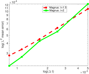
Fig. 1: Convergence of the implicit scheme for $\beta=1$, and $\beta=2$ in (154). The order of convergence in time is $0.57$ for $\beta=1$, $0.54$ for $\beta=2$. The total number of samples used is $100$.

In Figure 1, we can observe the convergence of the the stochastic Magnus scheme for two noise’s parameters. Indeed the order of convergence in time is $0.57$ for $\beta=1$ and $0.54$ for $\beta=2$. These orders are close to the theoretical orders $0.5$ obtained in Theorem 9 for $\beta=1$ and $\beta=2$.

References

- [1] H. AMANN, On abstract parabolic fundamental solutions, J. Math. Soc. Japan, 39 (1987), pp. 93-116.
- [2] S. BLANES, F. CASAS, J. A. OTEO, AND J. ROS, The Magnus expansion and some of its applications, Physics Reports, 470 (2009), pp. 151-238.
- [3] S. BLANES, F. CASAS, J. A. OTEO, AND J. ROS, Magnus and Fer expansion for matrix differential equations : the convergence problem, J. Phys. A. : Math. Gen., 31 (1998), pp. 259-268.
- [4] S. BLANES AND P. C. MOAN, Fourth- and sixth-order commutator-free Magnus integrators for linear and non-linear dynamical systems, Appl. Numer. Math., 56 (2006), pp. 1519-1537.
- [5] P. L. CHOW, Stochastic partial differential equations, Chapman & Hall/CRC. Appl. Math. Nonlinear Sci. ser., 2007.
- [6] P. G. CIARLET, The finite element method for elliptic problems, Amsterdam: North-Holland, 1978.
- [7] C. ELLIOT, AND S. LARSSON, Error estimates with smooth and nonsmooth data for a finite element method for the Cahn-Hilliard equation, Math. Comput. 58 (1992), pp. 603-630
- [8] L. C. EVANS, Partial Differential Equations, Grad. Stud., vol. 19, 1997.
- [9] H. FUJITA, AND T. SUZUKI, Evolutions problems (part1), in: P. G. Ciarlet and J. L. Lions(eds.), Handb. Numer. Anal., vol. II, North-Holland, (1991), pp. 789-928.
- [10] C. GONZÁLEZ, A. OSTERMANN, AND M. THALHMMER, A second-order Magnus-type integrator for non autonomous parabolic problems, J. Comput. Appl. Math., 189 (2006), pp. 142-156.
- [11] C. GONZÁLEZ, A. OSTERMANN, Optimal convergence results for Runge-Kutta discretizations of linear nonautonomous parabolic problems, BIT 39(1) (1999), pp. 79-95.
- [12] D. HENRY, Geometric Theory of semilinear parabolic equations, Lecture notes in Mathematics, vol. 840, Berlin : Springer, 1981.
- [13] D. HIPP, M. HOCHBRUCK, AND A. OSTERMANN, An exponential integrator for non-autonomous parabolic problems, Elect. Trans. on Numer. Anal., 41 (2014), pp. 497-511.
- [14] M. HOCHBRUCK, AND C. LUBICH, On Magnus integrators for time-dependent Schrödinger equations, SIAM. J. Numer. Anal., 41 (2003), pp. 945-963.
- [15] A. ISERLES, H. Z. MUNTHE-KASS, S. P. NØRSETT, AND A. ZANNA, Lie group methods, Acta Numer., 9 (2000), pp. 215-365.
- [16] A. JENTZEN, P. E. KLOEDEN, AND G. WINKEL, Efficient simulation of nonlinear parabolic SPDEs with additive noise, Ann. Appl. Probab., 21(3) (2011), pp. 908-950.
- [17] A. JENTZEN, AND M. RÖCKNER, Regularity analysis for stochastic partial differential equations with nonlinear multiplicative trace class noise, J. Differential Equations, 252 (2012), pp. 114-136.
- [18] P. E. KLOEDEN AND E. PLATEN, Numerical solutions of differential equations, Springer Verlag, 1992.
- [19] R. KRUSE, Optimal error estimates of Galerkin finite element methods for stochastic partial differential equations with multiplicative noise, IMA J. Numer. Anal., 34 (2014), pp. 217-251.
- [20] M. KOVÁCS, S. LARSSON, AND F. LINDGREN, Strong convergence of the finite element method with truncated noise for semilinear parabolic stochastic equations with additive noise, Numer. Algor., 53 (2010), pp. 309-220.
- [21] S. LARSSON, Nonsmooth data error estimates with applications to the study of the long-time behavior of the finite elements solutions of semilinear parabolic problems, Preprint 6, Departement of Mathematics, Chalmers University of Technology. http://www.math.chalmers.se/∼stig/papers/index.html (1992).
- [22] G. J. LORD AND A. TAMBUE, Stochastic exponential integrators for the finite element discretization of SPDEs for multiplicative and additive noise, IMA J. Numer. Anal., 33(2) (2012), pp. 515-543.
- [23] G. J. LORD, AND A. TAMBUE, A modified semi-implict Euler-Maruyama scheme for finite element discretization of SPDEs with additive noise, Appl. Math. Comput. 332 (2018), pp. 105-122.
- [24] Y. Y. LU, A fourth-order Magnus scheme for Helmholtz equation, J. Compt. Appl. Math., 173 (2005), pp. 247-253.
- [25] M. MAGNUS, On the exponential solution of a differential equation for a linear operator, Comm. Pure Appl. Math., 7 (1954), pp. 649-673
- [26] J. D. MUKAM AND A. TAMBUE, Strong convergence analysis of the stochastic exponential Rosenbrock scheme for the finite element discretization of semilinear SPDEs driven by multiplicative and additive noise, J. Sci. Comput. 74 (2018), pp. 937-978.
- [27] T. NAMBU, Characterization of the Domain of Fractional Powers of a Class of Elliptic Differential Operators with Feedback Boundary Conditions, J. Diff. Eq., 136 (1997), pp. 294-324.
- [28] A. PAZY, Semigroup of Linear Operators and Applications to Partial Differential Equations, Springer, new York, 1983.
- [29] D. G. PRATO AND J. ZABCZYK, Stochastic equations in infinite dimensions, Encyclopedia of Mathematics and its Applications, vol. 44, Cambridge : Cambridge University press, 1992.
- [30] C. PRÉVÔT AND M. RÖCKNER, A Concise Course on Stochastic Partial Differential Equations, Lecture Notes in Mathematics, vol. 1905, Springer, Berlin, 2007.
- [31] R. SEELY, Norms and domains of the complex powers , Amer. J. Math., 93 (1971), pp. 299-309.
- [32] J. SEIDLER, Da Prato-Zabczyk’s maximal inequality revisited I, Math. Bohem., 118(1) (1993), pp. 67-106.
- [33] A. TAMBUE AND J. D. MUKAM, Convergence analysis of the Magnus-Rosenbrock type method for the finite element discretization of semilinear non autonomous parabolic PDE with nonsmooth initial data, https://arxiv.org/abs/1809.03227v1, 2018
- [34] A. TAMBUE AND J. M. T. NGNOTCHOUYE, Weak convergence for a stochastic exponential integrator and finite element discretization of stochastic partial differential equation with multiplicative & additive noise, Appl. Numer. Math., 108 (2016), pp. 57-86.
- [35] H. TANABE, Equations of Evolutions, Pitman, London, 1979.
- [36] X. WANG, Strong convergence rates of the linear implicit Euler method for the finite element discretization of SPDEs with additive noise, IMA J. Numer. Anal., 37(2) (2017), pp. 965-984.
- [37] X. WANG AND Q. RUISHENG, A note on an accelerated exponential Euler method for parabolic SPDEs with additive noise, Appl. Math. Lett., 46 (2015), pp. 31-37
- [38] Y. YAN, Galerkin finite element methods for stochastic parabolic partial differential equations, SIAM J. Num. Anal., 43(4) (2005), pp. 1363-1384.