Convergence of jump processes with stochastic intensity to Brownian motion with inert drift

Abstract

Consider a random walker on the nonnegative lattice, moving in continuous time, whose positive transition intensity is proportional to the time the walker spends at the origin. In this way, the walker is a jump process with a stochastic and adapted jump intensity. We show that, upon Brownian scaling, the sequence of such processes converges to Brownian motion with inert drift (BMID). BMID was introduced by Frank Knight in 2001 and generalized by White in 2007. This confirms a conjecture of Burdzy and White in 2008 in the one-dimensional setting.

1 Introduction

Brownian motion with inert drift (BMID) is a process $X$ that satisfies the SDE

$$dX=dB+dL+KLdt,$$ (1)

where $K\geq 0$ is a constant and $L$ is the local time of $X$ at zero. This process behaves as a Brownian motion away from the origin but has a drift proportional to its local time at zero. Note that such a process is not Markovian because its drift depends on the past history. See Figure 1 for sample path comparisons between reflected Brownian motion and BMID. BMID can be constructed path-by-path from a standard Brownian motion via the employment of a Skorohod map. This is discussed in more detail in Section 2. We consider continuous time processes $(X_{n},V_{n})$ on $2^{-n}\mathbb{N}\times\mathbb{R}$ such that for $K\geq 0$,

1. $V_{n}(t):=K2^{n}\cdot Leb(0<s<t:X_{n}(s)=0)$ is the scaled time $X_{n}$ spends at the origin.
   

2. $X_{n}$ is a jump process with positive jump intensity $2^{2n}+2^{n}V_{n}(t)$ and downward jump intensity $2^{2n}$, modified appropriately so $X_{n}$ does not transition below zero.

The existence of such a process and its rigorous definition is presented in Section 3. Intuitively, $X_{n}$ is a random walker on the lattice $2^{-n}\mathbb{N}$ whose transition rates depend linearly on the amount of time the walker spends at zero. In other words, the positive jump rate of $X_{n}$ increases each time $X_{n}$ reaches zero. We show that as the lattice size shrinks to zero, i.e. as $n\to\infty$, $(X_{n},V_{n})$ converges in distribution to $(X,V)$, where $X$ is BMID and $V=KL$ is its velocity. See Theorem 4.4 and Corollary 4.5 for precise statements. By setting $K=0$ we recover the classical result that random walk on the nonnegative lattice converges to reflected Brownian motion.

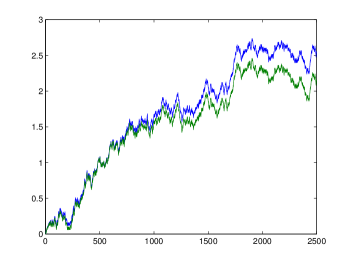
Figure 1: The figure shows a path of reflected Brownian motion and a path of BMID, each coming from the same Brownian sample path. This drift of BMID becomes evident as its domination over reflected Brownian motion grows with time. The drift of BMID comes from its contact with zero, which, in this figure, occurs in the beginning of the process.

1.1 Outline

In Section 2 we introduce BMID and its construction using Skorohod maps. We also give an equivalent formulation of the process $(X,V)$. In Section 3 we introduce the necessary background on jump process with stochastic intensity and introduce the setting used by Burdzy and White in [6]. Section 4 contains the statement and proof of the main results, Theorem 4.4 and Corollary 4.5. We conclude by briefly discussing BMID in a multidimensional setting in Section 5 .

1.2 Background

The study of BMID began in 2001 when Knight [11] described a Brownian particle reflecting above a particle with Newtonian dynamics. This two-particle system of Knight is equivalent in some sense to BMID in that the gap between the Brownian particle and the Newtonian particle is BMID. See Section 2. For more background on BMID see [13], where White constructs a multidimensional analog to BMID; [3], where Bass, Burdzy, Chen and Hairer study the stationary distribution; [1], where Barnes describes the hydrodynamic behavior of systems of Brownian motions with inert drift.

Burdzy and White studied similar processes from a discrete state point of view [6]. They consider a pair of processes $(X,L)$ with state space $\mathscr{L}\times\mathbb{R}^{d}$, where $\mathscr{L}$ is a finite set, and where the transition rate of $X$ depends on $L$, the scaled time $X$ has spent on previous states. See subsection 3.2 for definitions. The authors find necessary and sufficient conditions for such a process $(X,L)$ to have stationary distribution $\mu\times\gamma$, where $\mu$ is uniform on space and $\gamma$ is Gaussian. Burdzy and White make many conjectures involving approximating BMID, and its variants, and suggest the results of Bass, Burdzy, Chen, and Hairer [3] concerning a multidimensional analog of BMID stem from a discrete approximation scheme where the continuous process of BMID is a limit of these processes whose values take place in discretized space. The main result of this article confirms the discrete approximation scheme converges to the continuous model in the one dimensional setting.

BMID is just one example where a process with memory has a Gaussian stationary distribution. Gauthier [8] studies diffusions whose drift is also dependent on the process history through a linear combination of sine and cosine functions. He shows the average displacement across time obtains a Gaussian stationary distribution as time approaches infinity. In [2], Barnes, Burdzy, and Gauthier use this discrete approximation scheme, taking limits of Markov processes in the same class considered here, to demonstrate billiards with certain Markovian reflection laws have $\mu\times\gamma$ as the stationary measure for space and velocity, where as above $\mu$ is the uniform stationary measure in the spatial component and $\gamma$ the Gaussian stationary measure in the velocity component.

In Section 5 we briefly discuss a multidimensional analog of BMID that inspired conjectures of Burdzy and White.

2 An equivalent formulation of BMID

In this section we describe the process $(X,Y,V)$, where $X$ is Brownian motion reflecting from the inert particle $Y$ and where $Y$ has velocity $V$. We begin with a probability space $(\Omega,\mathbb{P},(\mathcal{F}_{t})_{t\geq 0})$, with the filtration $(\mathcal{F}_{t})_{t\geq 0}$ satisfying the usual conditions, supporting a Brownian motion $B$.

Theorem 2.1 (Existence and Uniqueness, Knight [11], White [13]).

Choose $K\geq 0$ and $v\in\mathbb{R}$. There exists a unique strong solution of continuous $\mathcal{F}_{t}$-adapted processes $(X,Y,V)$ satisfying:

$$\begin{split}&X(t)=B(t)+L(t),\text{ for all $t\geq 0$, almost surely,}\\ &X(t)\geq Y(t),\text{ for all $t\geq 0,$ almost surely,}\\ &dY=V(t)dt:=(v-KL(t))dt,\text{ for all $t\geq 0$, almost surely,}\\ &L\text{ is nondecreasing, and is flat away from the set }\{s:X(s)=Y(s)\}.\end{split}$$ (2)

Remark 2.2.

Flatness of $L$ off $\{s:X(s)=Y(s)\}$ means $\int_{0}^{\infty}\mathbf{1}(X(s)\neq Y(s))\,\mathrm{d}L(s)=0.$ One can use the Ito-Tanaka formula to show that $L$ is the local time of $X-Y$ at zero; see [13, Th. 2.7]. That is,

$$L(t)=\lim_{\epsilon\to 0}\frac{1}{2\epsilon}\int_{0}^{t}\mathbf{1}(|X(s)-Y(s)|<\epsilon)\,\mathrm{d}s,$$

where the right hand side is the local time of $X-Y$ at zero.

BMID together with its velocity is equivalent, in a certain sense, to the process $(X,Y,V)$ whose existence is given in Theorem 2.1. We will refer to the following result by Skorohod.

Lemma 2.3 (Skorohod, see [10]).

Let $f\in C([0,T],\mathbb{R})$ with $f(0)\geq 0.$ There is a unique, continuous, nondecreasing function $m_{f}(t)$ such that

$$x_{f}(t)=f(t)+m_{f}(t)\geq 0,$$

$$m_{f}(0)=0,\,m_{f}(t)\text{ is flat off }\{s:x_{f}(s)=0\},$$

that is given by

$$m_{f}(t)=\sup_{0<s<t}[-f(s)]\lor 0.$$

Remark 2.4.

The classical Lévy’s theorem states that for a Brownian motion $B$, $x_{B}$ is distributed as $|B|.$ See [10, Section 3.6C].

To see the equivalence between BMID and the process $(X,Y,V)$ from Theorem 2.1, consider the gap process $G(t)=X(t)-Y(t)$. Obviously $G\geq 0$, almost surely, and from (2) it follows that (when $v=0$)

$$dG=dB+dL+KLdt,$$ (3)

where $L$ is continuous, nondecreasing, and flat off $U^{-1}(0).$ From the comment in Remark 2.2 on local time, $G$ is a reflected diffusion whose drift is proportional to its local time at zero. Consequently, the gap process $G$ is BMID as it satisfies (1).

Assume we have a pair of processes $(U,V)$ adapted to a continuous filtration $\mathcal{F}_{t}$ that supports a Brownian motion $B$, and that for fixed $K\geq 0,v\in\mathbb{R}$

$$\begin{split}U(t)&=B(t)+\int_{0}^{t}V(x)\,\mathrm{d}x,\\ V(t)&=-v+KM^{U}(t),\\ M^{U}(t)&=\sup_{0<s<t}[-U(s)]\lor 0.\end{split}$$ (4)

In the system (4), it is clear from the definition of $M^{U}$ that $U+M^{U}\geq 0$ and it follows from the Skorohod Lemma 2.3 that $M^{U}$ is flat off the set $\{s:U(s)+M^{U}(s)=0\}.$ Therefore

$$B(t)+M^{U}\geq-\int_{0}^{t}V(s)\,\mathrm{d}s,$$

and $M^{U}$ is flat off of $\{s:B(t)+M^{U}=-\int_{0}^{t}V(s)\,\mathrm{d}s\}.$ Consequently,

$$\left(B(t)+M^{U}(t),-\int_{0}^{t}V(s)\,\mathrm{d}s,-V(t)\right)$$

satisfies the original equation (2) with respect to the filtration $\mathcal{F}_{t}$. Similarly, one can use the uniqueness statement in Skorohod’s Lemma to go from a solution of (4) to a solution of (2). This demonstrates the equivalence of the two systems (2) and (4) in the sense that if one solution exists for a given probability space $(\Omega,\mathbb{P},\mathcal{F}_{t})$, where $\mathcal{F}_{t}$ supports a given Brownian motion, then the other solution can be given by a path-by-path transformation.

Existence of a solution to (2) was first shown by Knight in [11]. A strong solution to a more general process was attained via the employment of a Skorohod map by David White [13] in a more general version of Theorem 2.5 given below.

Theorem 2.5 (White, [13]).

For every $f\in C([0,T],\mathbb{R}),K\geq 0,v\in\mathbb{R}$ there is a unique pair of continuous functions $(I,V)$ such that

$$\begin{split}x(t):=f(t)+I(t),\\ V(t)=v+Km(t),\\ I(t)=\int_{0}^{t}V(s)\,\mathrm{d}s,\\ m(t)=\sup_{0<s<t}[-x(s)\lor 0].\end{split}$$ (5)

Remark 2.6.

In Remark 2.4 it is mentioned that replacing the function $f$ with a Brownian motion in the formulation of Skorohod’s Lemma 2.3 gives rise to a representation of reflected Brownian motion. Similarly, when replacing $f$ in Theorem 2.5 pathwise by Brownian motion, the corresponding process $(x,-I,V)$ is a solution to (4). Note that Skorohod’s Lemma 2.3 implies that $m(t)$ in Theorem 2.5 is the unique monotonically increasing, continuous, function which is flat off of the level set $\{s:x(s)+m(s)=0\}$ such that $x+m$ is nonnegative.

Remark 2.7.

One can also see from the above arguments that $(U,V)$ of (4) solves

$$dU(t)=dB(t)+dL(t)+V(t)dt,\ dV(t)=KL(t)dt,\ V(0)=-v,$$

where $L$ is the local time of $U$ at zero.

3 Markov Processes with Memory

The title of this section seems contradictory because Markov processes lose their memory when conditioning on their current location. The processes considered are pairs of processes, one process taking values in “space,” and the other process storing the history of the space-valued process. The transition rate of the space-valued process depends on this stored history. We let $\mathcal{C}$ denote the class of such processes which we introduce more formally in this section. We will later construct a sequence of processes in $\mathcal{C}$ that will approximate BMID. First, we review well known facts of Poisson processes and point process with stochastic intensity. For reference, see Brémaud’s description of a doubly-stochastic point process in [5, Chapter 2].

3.1 Non-homogeneous Poisson processes

A non-homogeneous Poisson process with a nonnegative locally integrable rate (or intensity) function $\lambda(t)$ is a process $N$ such that

1. $N(0)=0$, a.s.

2. $N$ has independent increments,

3. $N$ is RCLL, a.s.

4. $N(a,b]=N(b)-N(a)\overset{d}{=}$ Poisson($\int_{a}^{b}\lambda(s)$).

If we let $T=\inf\{t:N(t)>0\}$ be the first jump time of $N$, then

$$\mathbb{P}(T>t)=\mathbb{P}(N(t)=0)=e^{-\int_{0}^{t}\lambda(s)\,\mathrm{d}s}.$$

Lemma 3.1.

Let $\lambda_{1},\lambda_{2}$ be two rate functions such that $\lambda_{1}(t)\leq\lambda_{2}(t)$ for all $t\geq 0$ and let $T_{1},T_{2}$ be the first jump time of their corresponding Poisson process. Then $T_{1}$ stochastically dominates $T_{2}.$

In [5, Chapter II], Brémaud discusses the notion of point processes adapted to a filtration $\mathcal{F}_{t}$ whose intensity $\lambda(s)$ is not a deterministic function but rather a process adapted to $\mathcal{F}_{t}$ with certain conditions.

Definition 3.2.

[5, II] Let $N_{t}$ be a point process adapted to the filtration $\mathcal{F}_{t}$ and let $\lambda_{t}$ be a nonnegative $\mathcal{F}_{t}$-progressive process such that $\int_{0}^{t}\lambda_{s}\,\mathrm{d}s<\infty$ almost surely for each $t\in[0,T]$. If

$$\mathbb{E}\left(\int_{0}^{\infty}C_{s}\,\mathrm{d}N_{s}\right)=\mathbb{E}\left(\int_{0}^{\infty}C_{s}\lambda_{s}\,\mathrm{d}s\right),$$ (6)

for all nonnegative $\mathcal{F}_{t}$-predictable processes $C_{t}$ then we say $N_{t}$ has stochastic intensity $\lambda_{t}.$

Remark 3.3.

In the proofs of later results we will refer to point processes with a given intensity or jump/step size. By a point process of jump/step size $a>0$ and (stochastic) intensity $\lambda$ we mean a process $aN_{t}$ where $N_{t}$ is a point process with (stochastic) intensity $\lambda.$ By the positive (resp. negative) jump process for a process we mean the process $aN_{t}$ (resp. $-aN_{t}$). For example, a process with jump size $2^{-n}$ with positive jump rate $\lambda_{1}(t)$, and negative jump rate $\lambda_{2}(t),$ is $2^{-n}(N_{1}-N_{2})$ where $N_{i}$ is a point process with (stochastic) rate $\lambda_{i}.$

Some well known facts of Poisson processes have analogous results for Poisson processes with stochastic intensities, which we list below.

Lemma 3.4.

Let $N_{1},N_{2}$ be two independent point processes with stochastic intensities $\lambda^{1},\lambda^{2}$ adapted to filtrations $\mathcal{F}^{1},\mathcal{F}^{2}$ respectively. Then $N_{1}+N_{2}$ is a point process with stochastic intensity $\lambda^{1}+\lambda^{2}$, adapted to $\mathcal{F}_{t}:=\sigma\left(\mathcal{F}^{1}_{t},\mathcal{F}^{2}_{t}\right).$

Sketch.

The fact that $N_{1},N_{2}$ are independent implies the two processes do not have common jumps, so that $(N_{1},N_{2})$ is a multivariate point process. The result follows from [5, T15, Chapter II.2]. ∎

Lemma 3.5.

Let $N_{1}$ be a point process with stochastic intensity $\lambda^{1}(t)\geq\lambda$, almost surely, for some $\lambda\in\mathbb{R}_{+}.$ Then we can enlarge the probability space to support a Poisson point process $N_{2}$ with constant intensity $\lambda$ and a point process $N_{3}$ of stochastic intensity $\lambda^{3}=\lambda^{1}-\lambda$ such that $N_{3}$ is independent of $N_{2}$ and $N_{2}+N_{3}$ has stochastic intensity $\lambda^{1}$.

Remark 3.6.

It is clear that one can generate a Poisson point process $N_{2}$ with constant intensity $\lambda$ which is independent of $N_{1}$. Lemma 3.5 could be generalized to include more general lower bounds than a constant, however, we don’t require this and sketch the proof only in the case when $N_{2}$ has constant intensity.

Sketch.

Enlarge the probability space to support two independent processes $N_{2}^{\prime},N_{3}^{\prime}$ where $N_{2}^{\prime}$ is a Poisson point process of rate $\lambda$ and $N_{3}^{\prime}$ is a point process with stochastic rate $\lambda^{3}=\lambda^{1}-\lambda.$ By Lemma 3.4, $N_{1}\overset{d}{=}N_{2}+N_{3}$, and the processes are adapted to the filtration generated by $(N_{1},N_{2},N_{3}).$ ∎

3.2 Class $\mathcal{C}$ of Markov Processes with Memory

As mentioned, Burdzy and White [6] study continuous time Markov processes $(X,L)$ on $\mathscr{L}\times\mathbb{R}$ where $\mathscr{L}=\{1,2,\dots,N\}$ is a finite set. For each $j\in\mathscr{L}$ we associate a vector $v_{j}\in\mathbb{R}$ and define $L_{j}(t)=Leb(0<s<t:X(s)=j)$ as the time $X$ has spent at location $j$ until time $t.$ We also define

$$L(t)=\sum_{j\in\mathscr{L}}v_{j}L_{j}(t)$$

as the accumulated time $X$ spends at each location, weighting the time spent at location $j$ by the factor $v_{j}$. The transition rates of $X$ will depend on $L(t).$ More precisely, we are given RCLL functions $a_{ij}:\mathbb{R}\to\mathbb{R}$ where $a_{ij}$ is the rate function for the Poisson process defining the transition of $X$ from $i$ to $j.$ Conditional on $X(t_{0})=i,L(t_{0})=l,$ the jump rate of $X$ transitioning from $i$ to $j$ is $a_{ij}(l+[t-t_{0}]v_{i})$ with $t\geq t_{0}.$ To construct such a process, for each $i$ we create independent random variables $(T_{i,j})_{j\in\mathscr{L}}$ which represents the jump time from $i$ to $j.$ Since this jump has intensity $a_{ij}(l+[t-t_{0}]v_{i})$ with $t\geq t_{0},$

$$\mathbb{P}(T_{i,j}>t+t_{0}|X(t_{0})=i,L(t_{0})=l)=\exp\left(-\int_{0}^{t}a_{ij}(l+sv_{i})\,\mathrm{d}s\right),$$ (7)

for all $t>0.$ Pick $j^{\prime}$ such that $T_{i,j^{\prime}}=\min_{j\neq i}T_{i,j}$, and define the first transition of $X$ after time $t_{0}$ to be location $j^{\prime}$ and occur at time $T_{i,j^{\prime}}.$

These dynamics can be produced from a collection of independent exponential random variables $(E_{i,j})_{i,j\in\mathbb{N}}$ of rate one. Set $T_{0}=0$ and recursively define

$$T_{i+1}^{j} =\inf\left(t>T_{i}:\int_{0}^{t}a_{X(T_{i})j}(L(T_{i})+v_{X(T_{i})(s-T_{i})})\mathrm{d}s>E_{i,j}\right)$$ (8)

$$T_{i+1} =\min_{j}T_{i+1}^{j}.$$ (9)

We use the convention $\inf\emptyset=\infty.$ Define

$$L(s) =L(T_{i})+v_{X_{n}(T_{i})}(s-T_{i}),\text{ for $s\in[T_{i},T_{i+1}]$}$$ (10)

$$X(s) =X(T_{i}),\text{ for $s\in[T_{i},T_{i+1})$}$$ (11)

$$X(T_{i+1}) =\text{argmin}_{j}T_{i+1}^{j}.$$ (12)

The pair $(X,L)$ is a strong Markov process with generator

$$Af(j,l)=v_{j}\cdot\nabla_{l}f(j,l)+\sum_{i\neq j}a_{ji}(l)[f(i,l)-f(j,l)],\ j=1,\dots,N,\ l\in\mathbb{R}.$$

Burdzy and White assume $(X,L)$ is irreducible in the sense that there is some $\{j_{0}\}\times U\subset\mathscr{L}\times\mathbb{R}$ such that

$$\mathbb{P}((X(t),L(t))\in\{j_{0}\}\times U|X(0)=i,L(0)=l)>0,\ \text{ for all $(i,l)\in\mathscr{L}\times\mathbb{R}$.}$$

It should be noted that although they consider $\mathscr{L}$ to be a finite set, their main results hold assuming that $\sup_{ij}a_{ij}(l)$ is bounded on compact sets of $l$ and $\sup_{i}|v_{i}|<\infty$. We denote $\mathcal{C}$ as the class of such processes with these conditions, allowing $\mathscr{L}=\mathbb{N}$.

4 Discrete Approximation

4.1 Definition of Processes

The reflected diffusion (1) describing BMID is a process whose drift depends on the local time of the diffusion at zero. Intuitively, to approximate this diffusion with a Markov process on the lattice $2^{-n}\mathbb{N}$ one would want the “velocity” to depend on the accumulated time spent at zero. This is modeled as a jump process whose intensity function is stochastic and depends linearly on the accumulated time the process spends at zero. These jump processes need to converge, as $n\to\infty$, to a process whose drift is the appropriate local time.

In Section 2 we introduced an equivalent formulation for BMID given by $(U,V)$ in (4). In this subsection we will describe two equivalent discrete processes that mirror the equivalence of the continuous processes described earlier; see Proposition 4.3. We do this because in order to prove the convergence result described in the introduction we actually prove the convergence result for the equivalent formulation.

Jump processes whose intensity depends linearly on the accumulated time at zero are described by the class $\mathcal{C}$ in subsection 3.2. Consider a process $(X_{n},V_{n}^{X})$ on the state space $2^{-n}\mathbb{N}\times\mathbb{R}$ where $v_{j}=0$ for all $j\neq 0,v_{0}=K2^{n}$ as given in the notation in that subsection. (We may hide the dependence on $n$ for convenience.) For an initial “velocity” $v\in\mathbb{R}$, we define

$$V_{n}^{X}(t)=-v+K2^{n}L_{n}(t)=-v+K2^{n}\cdot Leb(0<s<t:X_{n}(s)=0).$$

The rate functions $a_{ij}:\mathbb{R}\to\mathbb{R}$ are

$$\begin{split}a_{i(i+sign(l)2^{-n})}(l)&=2^{2n}+2^{n}|l|=2^{2n}+2^{n}|V_{n}^{X}(t)|,\\ a_{i(i-sign(l)2^{-n})}(l)&=2^{2n},\text{}\end{split}$$ (13)

where $l=V_{n}^{X}(t),$ except when $i=0$ where we do not allow a downward transition. By Lemma 3.4 the jump process $X_{n}$ can be decomposed into a sum of independent processes, $S_{n}$ and $Z_{n}$, whose rate functions sum to that of $X_{n}.$ The following definition will be used throughout the paper.

Definition 4.1.

For a process $Q(t)$ we define $M^{Q}(t)$ as the signed running minimum below zero of $Q$. That is,

$$M^{Q}(t)=\sup_{0<s<t}[-Q(s)]\lor 0.$$

Definition 4.2.

Consider the processes $(S_{n},Z_{n},V_{n})$ on $\left(2^{-n}\mathbb{Z}\right)^{2}\times\mathbb{R}$ where

1. $S_{n}$ is a continuous time simple random walk on $2^{-n}\mathbb{Z}$ with positive (and negative) jumps of size $2^{-n}$ and rate $2^{2n}.$

2. $Z_{n}$ is a point process with jump size $2^{-n}$ and with positive (resp. negative) jumps having stochastic and adapted rate $2^{n}|V_{n}|$ when $V_{n}>0$ (resp. $V_{n}<0$).

3. We have

   $$V_{n}(t)=-v+K2^{n}\cdot Leb(0<s<t:U_{n}(s)=-M_{n}(s)),$$

   $$U_{n}=S_{n}+Z_{n},$$

   $$M_{n}(t):=M^{U_{n}}(t).$$

That is, $S_{n}$ and $Z_{n}$ are point processes with adapted intensity functions as discussed in [5, Chapter 2].

Note the similarity to the equivalent formulation of BMID given by $(U,V)$ in (4) to $(U_{n},V_{n})$ given above. Existence of $(S_{n},Z_{n},V_{n})$ follows from the fact that it is of class $\mathcal{C}$, or, equivalently, one can construct the processes via the dynamics given in (8) by using the intensity functions (13).

Proposition 4.3.

The processes $(U_{n}+M_{n},V_{n})$ and $(X_{n},V_{n}^{X})$ have the same law.

Proof.

With these definitions $(U_{n}+M_{n},V_{n})$ has the same law as $(X_{n},V_{n}^{X})$ because it is of class $\mathcal{C}$ and satisfies (13). To see this, note that $V_{n}$ is adapted to the right continuous filtration $\mathcal{F}_{t}$ generated by the pair $(S_{n},Z_{n}).$ Also note that $U_{n}+M_{n}=S_{n}+Z_{n}+M_{n}$ is a nonnegative process on $2^{-n}\mathbb{N}$. By Lemma 3.4, $S_{n}+Z_{n}$ has a jump rate function of $2^{2n}+2^{n}V_{n}(t)$ where

$$V_{n}(t) =-v+K2^{n}\cdot Leb\{0<s<t:U_{n}(s)=-M_{n}(s)\}$$

$$=-v+K2^{n}\cdot Leb\{0<s<t:U_{n}(s)+M_{n}(s)=0\}.$$

Consequently, $V_{n}^{X}=V_{n}$ if we define $X_{n}:=U_{n}+M_{n}.$ Therefore $(U_{n}+M_{n},V_{n})$ is one realization of the process $(X_{n},V_{n}^{X})$ given by (13). ∎

We will work with $(S_{n},Z_{n},V_{n})$ as an equivalent formulation of $(X_{n},V_{n}^{X})$ defined by (13).

4.2 Theorem Statement

The main result of this article is that $(S_{n},V_{n},Z_{n},U_{n})$ converges in an appropriate sense to $(B,V,\int_{0}^{\cdot}V,U).$

Theorem 4.4.

For $K\geq 0$ and $v\in\mathbb{R}$, let $(S_{n},Z_{n},V_{n},U_{n})$ be given as in Definition 4.2 in subsection 4.1. Then

$$(S_{n},V_{n},Z_{n},U_{n})\overset{d}{\longrightarrow}(B,V,\int_{0}^{\cdot}V,U),$$

in the Skorohod topology on $D([0,T],\mathbb{R}^{4})$, where $(B,V,\int_{0}^{\cdot}V,U)$ is a quadruple of continuous processes adapted to the Brownian filtration of the first coordinate $B$ with the following holding for all $t\in[0,T]$, almost surely:

$$\begin{split}U(t)&=B(t)+\int_{0}^{t}V(x)\,\mathrm{d}x,\\ V(t)&=-v+KM^{U}(t),\\ \end{split}$$

and where $M^{U}$ is the running minimum given in Definition 4.1.

Theorem 4.4 has the following corollary.

Corollary 4.5.

Let $(X_{n},V_{n}^{X})$ be the process defined by (13) in subsection 4.1. Then

$$(X_{n},V_{n}^{X})\overset{d}{\longrightarrow}(X,V),$$

in the Skorohod topology on $D([0,T],\mathbb{R})$. Here $(X,V)$ is BMID together with its velocity. That is,

$$dX(t)=dB(t)+dL(t)+V(t)dt,\ dV(t)=KL(t)dt,V(0)=-v,$$ (14)

where $L$ is the local time of $X$ at zero.

Proof of Corollary.

By Proposition 4.3 we set $X_{n}:=U_{n}+M_{n}$ and $V_{n}^{X}:=V_{n}.$ Now Theorem 4.4 implies

$$(X_{n},V_{n}^{X})\overset{d}{\longrightarrow}(U,-v+KM^{U}),$$

and where $(U,-v+KM^{U})$ solves (14) as mentioned in Remark 2.7. ∎

Remark 4.6.

Let $D([0,T],\mathbb{R})$ denote the space of RCLL paths equipped with the Skorohod metric $d$ [7, Chapter 3 Section 5]. If a process $W_{n}$ with paths in $D([0,T],\mathbb{R})$ converges weakly to $W$, then according to the Skorohod representation, [7, Theorem 3.1.8], we can place $W_{n},W$ on the same probability space such that

$$d(W_{n},W)\longrightarrow 0,$$

almost surely. If the limiting process $W$ is continuous almost surely, then

$$\|W_{n}-W\|_{[0,T]}:=\sup_{0<s<T}|W_{n}(s)-W(s)|\longrightarrow 0,$$

almost surely on this probability space, and, in fact, uniform convergence and convergence in the Skorohod metric become equivalent. See Ethier and Kurtz, [7, Chapter 3 Section 5] and [7, Chapter 3 Section 10], and Billingsley [4, Chapter 3].

4.3 Proof of Theorem 4.4

In this section we prove Theorem 4.4 assuming the two lemmas below, one for tightness and the other for classifying the subsequential limits.

Lemma 4.7 (Tightness).

The collection of processes $\{(S_{n},Z_{n},V_{n}):n\in\mathbb{N}\}$ is tight in $D([0,T],\mathbb{R}^{2})$ $\times C[0,T]\subset D([0,T],\mathbb{R}^{3}).$ Because $U_{n}=S_{n}+Z_{n}$, it follows that $\{(S_{n},$ $V_{n},$ $Z_{n},U_{n}):n\in\mathbb{N}\}$ is also tight in $D([0,T],\mathbb{R})\times C[0,T]\times D([0,T],\mathbb{R}^{2})$. Furthermore, all limiting processes are continuous.

We prove Lemma 4.7 in Section 4.4. Assuming Lemma 4.7 holds, it remains to show there is a unique limit.

Lemma 4.8 (Classification of Limits).

Consider a subsequence $n_{k}$ with processes $(S_{n_{k}},$ $Z_{n_{k}},$ $V_{n_{k}},$ $U_{n_{k}})$ converging to $(S,Z,V,U)$ in $D([0,T],\mathbb{R}^{4})$ with the Skorohod topology. Then $(S,Z,V,U)$ is continuous and satisfies the equivalent formulation for BMID given in (4). That is,

1. $U(t)=S(t)+Z(t),$

2. $S(t)$ is a Brownian motion,

3. $V(t)=KL(t)-v,$ where $L(t)=\max_{0<s<t}[-U(s)]\lor 0,$

4. $\displaystyle Z(t)=\int\limits_{0}^{t}V(s)\,\mathrm{d}s.$

Lemma 4.8 is proved in Section 4.5.

Proof of Theorem 4.4.

Since the formulation of BMID described by $(B,V,U)$ in the statement of Theorem 4.4 is unique in law, Lemmas 4.7 and 4.8 characterizes the subsequential limits of $(S_{n},Z_{n},V_{n})$. See [13] where existence (and uniqueness) of such a system is proved. Consequently, we have convergence of the entire sequence to this equivalent formulation of BMID. ∎

4.4 Lemma 4.7: Tightness of $(S_{n},Z_{n},V_{n})$

Recall that our process $(S_{n},Z_{n},V_{n})$ is in $D([0,T],\mathbb{R}^{3})$, the space of RCLL paths with the Skorohod topology defined by the product metric $d\times d\times d$ where $d$ is the Skorohod metric, see Billingsley [4]. The following definition is taken from Jacod and Shiryaev [9].

Remark 4.9.

In general, it is not true that if $\alpha_{n}\to\alpha$, $\beta_{n}\to\beta$ in the Skorohod topology, then $\alpha_{n}+\beta_{n}\to\alpha+\beta.$ However, this does hold if either $\alpha$ or $\beta$ is continuous. See Jacod and Shiryaev [9, Proposition VI.1.23]. Similarly, by Remark 4.6 one can assume a sequence $(S_{n_{k}},Z_{n_{k}},V_{n_{k}})$ that converges in distribution on $D([0,T],\mathbb{R}^{3})$ in fact converges almost surely to a continuous process, say $(S^{\prime},Z^{\prime},V^{\prime})$ in the uniform metric if the limit is continuous; at least on some probability space. This immediately implies $U_{n_{k}}=S_{n_{k}}+Z_{n_{k}}$ converges almost surely to $S^{\prime}+Z^{\prime}.$

Definition 4.10.

[9, Definition VI.3.25] A sequence of processes $\{X_{i}:i\in\mathbb{N}\}$ in $D([0,T],\mathbb{R})$ is said to be $C$-tight if $\{X_{i}:i\in\mathbb{N}\}$ is tight on $D([0,T],\mathbb{R})$ and all limiting processes are continuous.

See Remark 4.6, which mentions the Skorohod metric when the limit processes are continuous. The proof that $(S_{n},Z_{n},V_{n})$ is tight is broken into multiple lemmas. Recall that $L_{n}(t):=2^{n}Leb(0<s<t:U_{n}(s)=-M_{n}(s))$ where $U_{n}:=S_{n}+Z_{n}$, $M_{n}:=M^{U_{n}},$ and $V_{n}:=-v+KL_{n}$.

Definition 4.11.

For $f\in D([0,T],\mathbb{R})$, let

$$\omega(f,\delta):=\sup_{\begin{subarray}{c}0<s<t<T\\ |t-s|<\delta\end{subarray}}|f(t)-f(s)|$$

be the modulus of continuity of $f.$

Recall that $\|f\|_{[a,b]}=\sup_{a<x<b}|f(x)|.$

Lemma 4.12.

[9, Proposition VI.3.26] A sequence of processes $X_{n}$ in $D([0,T],\mathbb{R})$ is $C$-tight if and only if for every $\epsilon>0$,

1. $\lim_{C\to\infty}\limsup_{n\to\infty}\mathbb{P}(\|X_{n}\|_{[0,T]}\geq C)=0$,
   

2. $\lim_{\delta\to 0}\limsup_{n\to\infty}\mathbb{P}(\omega(X_{n},\delta)>\epsilon)=0$.

Remark 4.13.

Notice that (i) follows from (ii) and $\lim_{C\to\infty}\limsup_{n\to\infty}\mathbb{P}(|X_{n}(0)|>C)=0.$ To see this, take $\delta=1$ and $\epsilon=C/2$ so that by definition of the modulus of continuity

$$\|X_{n}\|_{[0,T]}\leq|X_{n}(0)|+\sum_{i=1}^{T}\omega(X_{n},1).$$

Consequently, the triangle inequality gives

$$\mathbb{P}(\|X_{n}\|_{[0,T]}>C) \leq\mathbb{P}(|X_{n}(0)|+\lceil T\rceil\omega(X_{n},1)>C)$$

$$\leq\mathbb{P}(|X_{n}(0)|>C/2)+\mathbb{P}(\omega(X_{n},1)>C/(2\lceil T\rceil)),$$

where $\lceil r\rceil$ is the smallest integer larger than $r,$ from which it is clear that (ii) and $\lim_{C\to\infty}\limsup_{n\to\infty}\mathbb{P}(|X_{n}(0)|>C)=0$ imply (i).

Lemma 4.14.

Assume that the sequences of processes $(X_{n}),(X^{\prime}_{n}),(X^{\prime\prime}_{n})$ in $D([0,T],\mathbb{R})$ satisfy

$$X^{\prime}_{n}(t)-X^{\prime}_{n}(s)\leq X_{n}(t)-X_{n}(s)\leq X^{\prime\prime}_{n}(t)-X^{\prime\prime}_{n}(s),\ \ 0\leq s\leq t,$$

almost surely. If both $(X_{n}^{\prime})$ and $(X_{n}^{\prime\prime})$ are $C$-tight, then $(X_{n})$ is also $C$-tight.

Proof.

For any $C>0$, the triangle inequality gives

$$\mathbb{P}(\|X_{n}\|_{[0,T]}>C)\leq\mathbb{P}(\|X_{n}^{\prime}\|_{[0,T]}>C/2)+\mathbb{P}(\|X_{n}^{\prime\prime}\|_{[0,T]}>C/2),$$

which verifies condition (i) in the statement of Lemma 4.12 by taking $\lim_{C\to\infty}$ $\limsup_{n\to\infty}$ of both sides. Similarly, for every $\delta,\epsilon>0,$

$$\mathbb{P}(\omega(X_{n},\delta)>\epsilon)\leq\mathbb{P}(\omega(X_{n}^{\prime},\delta)>\epsilon/2)+\mathbb{P}(\omega(X_{n}^{\prime\prime},\delta)>\epsilon/2),$$

and taking $\lim_{\delta\to 0}\limsup_{n\to\infty}$ on both sides verifies condition (ii) in the statement of Lemma 4.12. ∎

The following two lemmas are classical and we omit proofs.

Lemma 4.15.

Let $X\overset{d}{=}Exp(\lambda),Y\overset{d}{=}Exp(\mu)$ be independent. Then $X\land Y\overset{d}{=}Exp(\lambda+\mu)$ is independent from $W=1_{\{X\land Y=X\}}$. In other words, the minimum of two independent exponential random variables is independent from which exponential r.v. occurred first.

Lemma 4.16.

Fix $a>0$, and for each $n\in\mathbb{N}$ let $N_{n}$ be a Poisson process with intensity $\alpha 2^{n}$. Then $\{2^{-n}N_{n}(t):t\in[0,T]\}$ converges in distribution to the line $g(t)=at$, in the space $D([0,T],\mathbb{R})$. In particular $\{2^{-n}N_{n}(t):t\in[0,T],n\in\mathbb{N}\}$ is $C$-tight.

Lemma 4.17.

There is a filtered probability space $(\Omega,(\mathcal{F}_{t})_{t\geq 0},\mathbb{P})$ satisfying the usual conditions, supporting the $\mathcal{F}_{t}$-adapted process $(S_{n},Z_{n},V_{n})$ given in Definition 4.2, also supporting the $\mathcal{F}_{t}$-adapted process $(U_{n}^{\prime},Z_{n}^{\prime},L_{n}^{\prime})$, such that

$$U_{n}^{\prime} =S_{n}+Z_{n}^{\prime},$$

$$M_{n}^{\prime} =M^{U_{n}^{\prime}},$$

$$L_{n}^{\prime}(t) =2^{n}Leb(0<s<t:U_{n}^{\prime}=-M_{n}^{\prime}).$$

Here $Z_{n}^{\prime}$ is a Poisson point process of intensity $|v2^{n}|$ and jump size $sign(v)2^{-n}$. Furthermore,

$$Z_{n}^{\prime}(t)-Z_{n}^{\prime}(s)\leq Z_{n}(t)-Z_{n}(s),$$ (15)

for all $0\leq s\leq t\leq T$, almost surely, and

$$0\leq L_{n}(t)-L_{n}(s)\leq L_{n}^{\prime}(t)-L_{n}^{\prime}(s),$$ (16)

for all $0\leq s\leq t\leq T$, almost surely. The construction will yield independence between $Z_{n}^{\prime}$ and $S_{n}.$

Proof.

By definition $V_{n}\geq-v$ almost surely. Recall that $Z_{n}$ is a point process with stochastic intensity $|2^{n}V_{n}|$ and jump size $sign(V_{n})2^{-n}$, so by Lemma 3.5 we assume the probability space included a process $Z_{n}^{\prime}$ with downward stochastic jump intensity $|v2^{n}|$ and step size $2^{-n}$ such that

$$Z_{n}^{\prime}(t)-Z_{n}^{\prime}(s)\leq Z_{n}(t)-Z_{n}(s)$$

for all $0\leq s\leq t\leq T,$ almost surely. This inequality holds because the negative transitions of $Z$ will have a rate less than $|v|2^{n}$, which is the transition rate for negative jumps of $Z_{n}^{\prime}$. (And by definition $Z_{n}^{\prime}$ makes negative jumps only.) The jump times of $Z_{n}^{\prime}$ are independent of $S_{n}$ hence the processes are independent. This demonstrates (15). It follows that

$$U_{n}:=S_{n}+Z_{n}\geq S_{n}+Z_{n}^{\prime}=:U_{n}^{\prime},$$

almost surely. Notice both processes $U_{n}+M_{n},U_{n}^{\prime}+M_{n}^{\prime}$ transition as a continuous time (nonnegative) random walk but with an additional “drift” process of $Z_{n},Z_{n}^{\prime}$ respectively. For instance, a transition of $U_{n}$ beginning from its running minimum corresponds to a transition from zero for the walk $U_{n}+M_{n}$. By (15), the process $U_{n}+M_{n}^{U}$ dominates that of $U_{n}^{\prime}+M_{n}^{U^{\prime}}$. That is,

$$U_{n}+M_{n}\geq U_{n}^{\prime}+M_{n}^{\prime}\geq 0,\text{ almost surely.}$$ (17)

Hence, $U_{n}^{\prime}+M_{n}^{\prime}$ is zero whenever $U_{n}+M_{n}$ is zero. Consequently, $\{s<z<t:U_{n}^{\prime}(z)=-M_{n}^{\prime}(z)\}\subset\{z:s<z<t,U_{n}(z)=-M_{n}(z)\}$ for every $(s,t)\subset[0,T],$ almost surely. Therefore,

$$0\leq L_{n}(t)-L_{n}(s)\leq L_{n}^{\prime}(t)-L_{n}^{\prime}(s),$$ (18)

for every $(s,t)\subset[0,T]$, almost surely, demonstrating (16). ∎

Lemma 4.18.

For every $T>0,$ $\mathbb{E}(M_{n}(T))\leq\mathbb{E}(M_{n}^{\prime}(T))\leq 2\sqrt{2T+T|v|\sqrt{2T}+2|v|T}$ where $v$ is the initial value of $V_{n}$ and $M_{n}^{\prime}$ is defined in Lemma 4.17.

Proof.

According to Lemma 4.17 we assume our probability space supports $(S_{n},Z_{n},V_{n})$ as well as the $Z_{n}^{\prime}$ given in that lemma’s statement. Consequently,

$$U_{n}:=S_{n}(t)+Z_{n}(t)\geq S_{n}(t)+Z_{n}^{\prime}(t)=:U_{n}^{\prime},$$

for all $t\in[0,T]$, almost surely, implying

$$M_{n}(T):=M^{U_{n}}(T)\leq M^{U_{n}^{\prime}}(T)=:M_{n}^{\prime}(T),$$ (19)

almost surely. We can express the continuous time random walk $S_{n}$ as $2^{-n}(N_{1}(t)-N_{2}(t))$ where $N_{i}$ are independent Poisson processes of rate $2^{2n}$, and consequently $\mathbb{E}(S_{n}(T)^{2})=\mathrm{Var}(S_{n}(T))=2^{-2n}(\mathrm{Var}(N_{1}(T))+\mathrm{Var}(N_{2}(T)))=2T.$ By Cauchy-Schwarz this yields $\mathbb{E}|S_{n}(T)|\leq\sqrt{2T}.$ By Doob’s Martingale inequality, the fact that $Z_{n}^{\prime}(T)$ is distributed as $-2^{-n}$ $\text{Poisson}(|v2^{n}T|)$, and independence of $Z_{n}^{\prime}$ and $S_{n}$, we compute

$$\mathbb{E}(M_{n}(T)) \overset{\eqref{eq:Bound_M_n}}{\leq}\mathbb{E}(M_{n}^{\prime}(T))$$

$$\leq\sqrt{\mathbb{E}(M_{n}^{\prime}(T)^{2})},\text{ Cauchy-Schwarz}$$

$$\leq\sqrt{4\mathbb{E}(U_{n}^{\prime}(T)^{2})}=2\sqrt{\mathbb{E}(|S_{n}(T)+Z_{n}^{\prime}(T)|^{2})},\text{by Doob's Maximal Inequality}$$

$$\leq 2\sqrt{\mathbb{E}(S_{n}^{2}(T))+\mathbb{E}|S_{n}(T)Z_{n}^{\prime}(T)|+\mathbb{E}(Z_{n}^{\prime}(T)^{2})}\leq 2\sqrt{2T+T|v|\sqrt{2T}+2|v|T}.$$

∎

Lemma 4.19.

In the notation of Lemma 4.17, $L_{n}^{\prime}$ converges in distribution to $M^{B^{-v}}$ in the space $C([0,T],\mathbb{R})$ with the uniform norm. Here, $B^{-v}(t):=B(t)-vt$ where $B$ is a Brownian motion. In particular, $\{L_{n}^{\prime}:n\in\mathbb{N}\}$ is $C$-tight. Furthermore, $\sup_{n}\mathbb{E}L_{n}(T)\leq\sup_{n}\mathbb{E}L_{n}^{\prime}(T)<\infty$.

Proof.

We begin by showing the weak convergence for which we use a similar technique in the proof of Lemma 4.8 (iii). We record the amount of time $U_{n}^{\prime}$ spends at each level of the running minimum, and express $L_{n}^{\prime}(t)$ as the sum of these times. By Lemma 4.16, $Z_{n}^{\prime}(t)=-2^{-n}N_{n}(t)$ converges in distribution to $g(t)=-vt$ in the space $D([0,T],\mathbb{R})$. By Donsker’s theorem, $S_{n}$ converges in distribution to a Brownian motion $B$ and consequently $U_{n}^{\prime}:=S_{n}+Z_{n}^{\prime}$ converges in distribution to $B+g=:U^{\prime}.$ This implies $M_{n}^{\prime}:=M^{U_{n}^{\prime}}$ converges to $M^{U^{\prime}}$ in distribution because $f\mapsto M^{f}$ is continuous in the uniform norm and the limiting processes are continuous. See Remark 4.9. Note that $2^{n}M_{n}^{\prime}(t)+1$ is the number of levels the running minimum of $U_{n}^{\prime}$ has reached by time $t.$ Let $\tau^{(j)}=\inf\{t>0:U_{n}^{\prime}(t)=-j2^{-n}\}$, so that $\tau^{(j)}$ is the first time $M_{n}^{\prime}$ reaches $j2^{-n}.$ Define

$$T_{j}:=Leb(s\geq\tau^{(j)}\mid-U_{n}^{\prime}(s)=M_{n}^{\prime}(s)=j2^{-n}).$$

Then,

$$\begin{split}2^{n}\sum_{j=0}^{2^{n}M_{n}^{\prime}(s)}T_{j}&\leq L_{n}^{\prime}(s)\leq 2^{n}\sum_{j=0}^{2^{n}M_{n}^{\prime}(s)+1}T_{j},\end{split}$$ (20)

for all $s\in[0,T]$, almost surely. When $M_{n}^{\prime}=j2^{-n}$, after the process $U_{n}^{\prime}$ arrives at $-j2^{-n}$ for the $k$th time, it makes a positive jump upon the arrival of an $Exp(2^{2n})$ random variable, call it $\mu_{k}^{(j)}$, while it makes a negative jump upon the arrival of an $Exp(2^{2n}+|v2^{n}|)$ random variable $\mu_{k}^{(j)^{\prime}}$. Consider the pair $(\mu_{k}^{(j)}\land\mu_{k}^{(j)^{\prime}},I_{j})$ where $I_{j}=1_{\{\mu_{k}^{(j)}\land\mu_{k}^{(j)^{\prime}}=\mu_{k}^{(j)}\}}$. By Lemma 4.15, $I_{j}$ is independent from the i.i.d. sequence $(\mu_{k}^{(j)}\land\mu_{k}^{(j)^{\prime}}:k\geq 1)$. Then, $W_{j}:=\inf\{k:I_{k}=0\}$ is the number of times $U_{n}^{\prime}$ visits $-j2^{-n}$ while the signed running minimum $M_{n}^{\prime}$ is $j2^{-n}$. Because $I_{j}\overset{d}{=}\text{Bernoulli}(p)$ with

$$p=\frac{2^{2n}}{2^{2n+1}+v2^{n}},$$

and $W_{j}$ is Geometrice$(p)$ (since it is the first time this sequence of Bernoulli random variables is zero), and Lemma 4.15 implies that $W_{j}$ is independent of $\mu_{i}^{(j)},\mu_{i}^{(j)^{\prime}}$. Thus,

$$T_{j}=\sum_{i=1}^{W_{j}}\mu_{i}^{(j)}\land\mu_{i}^{(j)^{\prime}}$$

is a Geometric sum of i.i.d. exponential random variables of rate $\lambda=2^{2n+1}+v2^{n}$ that are independent of the number of the sums $W_{j}$. Such a sum is exponential of rate $p\lambda$. That is, $T_{j}\overset{d}{=}Exp(p\lambda)=Exp(2^{2n})$. Each $T_{j}$ is measurable with respect to $\sigma\{(U_{n}^{\prime}(s),M_{n}^{\prime}(s)):s\in(\tau^{(j)},\tau^{(j+1)}]\},$ and $(T_{j}:j\geq 1)$ is independent of $(U_{n}^{\prime}(\tau^{(j)}),M_{n}^{\prime}(\tau^{(j)}))$. (In other words, $T_{j}$ depends only on the excursions between the stopping times and not the initial position.) Thus $(T_{j}:j\geq 1)$ is a sequence of i.i.d. $Exp(2^{2n})$ random variables. We show the left hand side of (20) converges in probability to $M^{\prime}(s)$ in the uniform norm for $s\in[0,T]$. The proof for the right hand side is essentially identical. Without loss of generality, we may assume $M_{n}^{\prime}$ converges almost surely to $M^{\prime}$ by the Skorohod representation theorem and the fact shown above that $M_{n}^{\prime}$ converges to $M^{\prime}$ in distribution. Therefore

$$\sup_{s\in[0,T]}\left|\sum_{j=0}^{2^{n}M_{n}^{\prime}(s)}2^{-n}-M^{\prime}(s)\right|\longrightarrow 0,\text{ almost surely.}$$

To show the sequence $\displaystyle 2^{n}\sum_{j=0}^{2^{n}M_{n}^{\prime}(s)}T_{j},n\geq 1,$ converges in probability to $M^{\prime}(s)$ uniformly for $s\in[0,T],$ it suffices to show

$$\sup_{s\in[0,T]}\left|2^{n}\sum_{j=0}^{2^{n}M_{n}^{\prime}(s)}T_{j}-\sum_{j=0}^{2^{n}M_{n}^{\prime}(s)}2^{-n}\right|\overset{\mathbb{P}}{\longrightarrow}0.$$

Because $T_{j}\overset{d}{=}\text{Exp}(2^{2n})$, we know $z_{j}:=2^{n}T_{j}\overset{d}{=}\text{Exp}(2^{n}).$ Then,

$$2^{n}\sum_{j=0}^{2^{n}M_{n}^{\prime}(s)}T_{j}-\sum_{j=0}^{2^{n}M_{n}^{\prime}(s)}2^{-n}=\sum_{j=0}^{2^{n}M_{n}^{\prime}(s)}(z_{j}-2^{-n}),$$

where $z_{j}-2^{-n}$ are i.i.d. mean zero random variables with variance $2^{-2n}$. By Kolmogorov’s maximal inequality, for each $C,\epsilon>0$

$$\mathbb{P}\left(\sup_{s\in[0,T]}\left|\sum_{j=0}^{2^{n}M_{n}^{\prime}(s)}(z_{j}-2^{-n})\right|>\epsilon\right)$$

$$\leq\mathbb{P}\left(\sup_{1\leq k\leq 2^{n}C}\left|\sum_{j=0}^{k}(z_{j}-2^{-n})\right|>\epsilon\right)+\mathbb{P}(M_{n}^{\prime}(T)>C)$$

$$\leq\epsilon^{-2}\mathrm{Var}\left(\sum_{j=0}^{2^{n}C}(z_{j}-2^{-n})\right)+\mathbb{P}(M_{n}^{\prime}(T)>C)$$

$$\leq\epsilon^{-2}2^{n}C2^{-2n}+\mathbb{P}(M_{n}^{\prime}(T)>C).$$

Because $M_{n}^{\prime}$ converges to $M^{\prime}$ almost surely, this implies

$$\limsup_{n\to\infty}\mathbb{P}\left(\sup_{s\in[0,T]}\left|\sum_{j=0}^{2^{n}M_{n}^{\prime}(s)}(z_{j}-2^{-n})\right|>\epsilon\right)$$

$$\leq\limsup_{n\to\infty}\mathbb{P}(M_{n}^{\prime}(T)>C)$$

$$=\mathbb{P}(M^{\prime}(T)>C),$$

where $C>0$ is arbitrary. Since $M^{\prime}(T)$ is finite a.s., $\mathbb{P}(M^{\prime}(T)>C)$ can be made arbitrarily small with a large choice for $C$. Hence

$$\sup_{s\in[0,T]}\left|\sum_{j=0}^{2^{n}M_{n}^{\prime}(s)}(z_{j}-2^{-n})\right|\overset{\mathbb{P}}{\longrightarrow}0,$$

and the left hand side of (20) converges in probability to $M^{\prime}$. That is,

$$\sup_{s\in[0,T]}\left|2^{n}\sum_{j=0}^{2^{n}M_{n}^{\prime}(s)}T_{j}-M^{\prime}(s)\right|\overset{\mathbb{P}}{\longrightarrow}0.$$ (21)

The convergence in probability for the right hand side is similar,

$$\sup_{s\in[0,T]}\left|2^{n}\sum_{j=0}^{2^{n}M_{n}^{\prime}(s)+1}T_{j}-M^{\prime}(s)\right|\overset{\mathbb{P}}{\longrightarrow}0.$$ (22)

Because (20) is an almost sure bound,

$$\mathbb{P}\Big{(}\sup_{s\in[0,T]}|L_{n}^{\prime}(s)-M^{\prime}(s)|>\epsilon\Big{)}$$

$$\leq\mathbb{P}\left(\sup_{s\in[0,T]}\left|2^{n}\sum_{j=0}^{2^{n}M_{n}^{\prime}(s)}T_{j}-M^{\prime}(s)\right|>\epsilon/2\right)+\mathbb{P}\left(\sup_{s\in[0,T]}\left|2^{n}\sum_{j=0}^{2^{n}M_{n}^{\prime}(s)+1}T_{j}-M^{\prime}(s)\right|>\epsilon/2\right),$$

and taking $\limsup_{n\to\infty}$ on both sides, (21) and (22) imply

$$\limsup_{n\to\infty}\mathbb{P}\Big{(}\sup_{s\in[0,T]}|L_{n}^{\prime}(s)-M^{\prime}(s)|>\epsilon\Big{)}=0,$$

for every $\epsilon>0.$ This complete the proof that $L_{n}^{\prime}$ converges in probability to $M^{\prime}$ in the uniform norm. Since $M^{\prime}$ is a continuous process, the sequence $\{L_{n}^{\prime}:n\in\mathbb{N}\}$ is $C$-tight; see Definition 4.10.

To demonstrate the uniform moment bound, note that $L_{n}(T)\leq L_{n}^{\prime}(T)$, equation (20), and Wald’s lemma imply

$$\mathbb{E}(L_{n}(T))\leq\mathbb{E}(L_{n}^{\prime}(T))=\mathbb{E}(M_{n}^{\prime}(T))+2^{-n}.$$

Applying the uniform moment bound on $M_{n}^{\prime}(T)$ given in Lemma 4.18, we see

$$\sup_{n}\mathbb{E}(L_{n}(T))\leq\sup_{n}\mathbb{E}(L_{n}^{\prime}(T))\leq\sup_{n}\mathbb{E}(M_{n}^{\prime}(T))+1<\infty.$$

∎

Corollary 4.20.

The collection of processes $\{L_{n}:n\in\mathbb{N}\}$ is $C$-tight.

Proof.

This follows directly from (18), the fact that $\{L_{n}^{\prime}:n\in\mathbb{N}\}$ is $C$-tight by Lemma 4.19 (and that the zero process is trivially $C$-tight), and Lemma 4.12. ∎

Lemma 4.21.

The collection of processes $\{Z_{n}:n\in\mathbb{N}\}$ is $C$-tight.

Proof.

We will use a localization argument by stopping the stochastic intensity of $Z_{n}$ when it becomes large. Recall that $|2^{n}V_{n}|$ is the stochastic intensity of $Z_{n}.$ For $C>v\geq 0$ set

$$T_{C}^{n}=\inf\{t>0:V_{n}(t)>C\}=\inf\left\{t>0:L_{n}(t)>\frac{v+C}{K}\right\}.$$

Define a process $\widetilde{Z}_{n}$ such that $\widetilde{Z}_{n}|_{[0,T_{C}^{n}]}=Z_{n}|_{[0,T_{C}^{n}]}$, almost surely, while after time $T_{C}^{n}$ let $\widetilde{Z}_{n}$ have positive jump intensity $C2^{n}$ and jump size $2^{-n}$ (and make only positive jumps). By Lemma 3.5 we can stochastically dominate the number of transitions made by $\widetilde{Z}_{n}$ in a given time interval by the number of transitions made by a point process $Z^{1}_{n}(t)$ of intensity $C2^{n}$ and jump size $2^{-n}$ (in the same time interval). More precisely, we may assume there exists a process $Z^{1}_{n}(t)=2^{-n}N(C2^{n}t)$ on our probability space, where $N$ is Poisson process of unit intensity, and

$$0\leq|Z_{n}(t)-Z_{n}(s)|\leq|Z_{n}^{1}(t)-Z_{n}^{1}(s)|$$ (23)

for every interval $(s,t)\subset[0,T_{C}^{(n)}],$ almost surely. By monotonicity of $Z_{n}^{1}$ and Doob’s maximal inequality, for fixed $\epsilon,\delta,C>0$ we have

$$\mathbb{P}\Big{(}\sup_{t\in[0,T-\delta]}\sup_{t<u,v<t+\delta}|Z_{n}(u)-Z_{n}(v)|>\epsilon\Big{)}$$

$$\leq\mathbb{P}\Big{(}\sup_{t\in[0,T-\delta]}\sup_{t<u,v<t+\delta}|\widetilde{Z}_{n}(u)-\widetilde{Z}_{n}(v)|>\epsilon,T_{C}^{(n)}>T\Big{)}+P(T_{C}^{(n)}<T)$$

$$\leq\mathbb{P}\Big{(}\sup_{t\in[0,T-\delta]}\sup_{t<u,v<t+\delta}|Z_{n}^{1}(u)-Z_{n}^{1}(v)|>\epsilon\Big{)}+P(T_{C}^{(n)}<T)$$

$$=\mathbb{P}\Big{(}\sup_{t\in[0,T-\delta]}|Z_{n}^{1}(t+\delta)-Z_{n}^{1}(t)|>\epsilon\Big{)}+P(V_{n}(T)>C)$$

$$\leq\mathbb{P}\Big{(}\sup_{t\in[0,T-\delta]}|Z_{n}^{1}(t+\delta)-Z_{n}^{1}(t)|>\epsilon\Big{)}+\frac{|v|+K\sup_{n}\mathbb{E}(L_{n}(T))}{C}.$$

By Lemma 4.16 and Lemma 4.12 we know

$$\lim_{\delta\to 0}\limsup_{n\to\infty}\mathbb{P}\Big{(}\sup_{t\in[0,T-\delta]}|Z_{n}^{1}(t+\delta)-Z_{n}^{1}(t)|>\epsilon\Big{)}=0.$$

By this and the uniform moment bound of $\sup_{n}\mathbb{E}(L_{n}(T))$ in Lemma 4.19, there exists a constant $A$ independent of $C,\epsilon,n$ such that

$$\lim_{\delta\to 0}\limsup_{n\to\infty}\mathbb{P}\Big{(}\sup_{t\in[0,T-\delta]}\sup_{t<u,v<t+\delta}|Z_{n}(u)-Z_{n}(v)|>\epsilon\Big{)}\leq\frac{A}{C}.$$

By choosing $C$ arbitrarily large, we see

$$\lim_{\delta\to 0}\limsup_{n\to\infty}\mathbb{P}\Big{(}\sup_{t\in[0,T-\delta]}\sup_{t<u,v<t+\delta}|Z_{n}(u)-Z_{n}(v)|>\epsilon\Big{)}=0.$$

Hence $Z_{n}$ satisfies (ii) of Lemma 4.12. Condition (i) follows from Remark 4.13 and the fact that $Z_{n}(0)=0$ almost surely. This completes our verification of conditions (i)-(ii) of Lemma 4.12 sufficient for $C$-tightness of $\{Z_{n}:n\in\mathbb{N}\}$. ∎

Corollary 4.22.

The collection of processes $\{(S_{n},Z_{n},V_{n}):n\in\mathbb{N}\}$ is $C$-tight in $D([0,T],\mathbb{R}^{3})$ with the Skorohod topology.

Remark 4.23.

As topological spaces, $D([0,T],\mathbb{R}^{d})$ with the Skorohod topology is not equivalent to $D([0,T],\mathbb{R})^{d}$ with the product topology. However, because the marginals are $C$-tight this a non-issue essentially because uniform convergence to a continuous function becomes the same in both spaces. See the comment in Jacod and Shiryaev [9, VI.1.21].

Proof.

Note that $S_{n}$ is $C$-tight by Donsker’s theorem, while $C$-tightness of $V_{n}=v-KL_{n}$, and $Z_{n}$, follow from Corollary 4.20, and Lemma 4.21, respectively. By Skorohod’s representation theorem, every subsequence of $(S_{n},Z_{n},V_{n})$ converging to a limiting process $(S,Z,V)$ can be assumed to converge almost surely in the product metric $d\times d\times d$, the product metric on $D([0,T],\mathbb{R})^{3}$. By $C$-tightness of the marginals, $S,Z,V$ are all continuous, so that $(S,Z,V)$ is a continuous process. As in Remark 4.6, this implies the subsequence of $(S_{n},Z_{n},V_{n})$ converges to $(S,Z,V)$ almost surely in the uniform norm, which implies almost sure convergence in $D([0,T],\mathbb{R}^{3})$ under the Skorohod metric. Thus, $(S_{n},Z_{n},V_{n})$ is $C$-tight as a collection of processes with paths in $D([0,T],\mathbb{R}^{3})$. ∎

4.5 Lemma 4.8: Characterization of subsequential limits

We prove items (i)-(iv) in Lemma 4.8 separately. The proof of (iii) was inspired by the proof of Lévy’s theorem given in [12, Chapter 6], where the authors essentially note the equivalence of the processes $(U_{n}+M_{n},V_{n})$ and $(X_{n},V_{n}^{X})$, which we described in subsection 4.1, for the case $K=0.$ Lévy’s theorem is the statement that $(L,|B|)$ and $(M^{B},B+M^{B})$ yield the same distribution on $C([0,T],\mathbb{R}^{2}).$ Here $L$ is the local time of $|B|$ at zero. See [10, Chapter 3.6] for a detailed statement.

Proof of (i).

This follows trivially from the definition of $U_{n}=S_{n}+Z_{n}.$ ∎

Proof of (ii).

Recall $S_{n}$ is a continuous time scaled simple random walk. Since $S_{n_{k}}$ converges to $S$, $S$ is a Brownian motion by Donsker’s theorem. ∎

We give a brief heuristic for the proof of (iii). Recall $L_{n}=2^{n}\cdot Leb(0<s<t:U_{n}(s)=-M_{n}(s))$ and $V_{n}=-v+KL_{n}.$ Each time $M_{n}$ increases, $U_{n}$ will make approximately a Geometric($1/2$) number of visits to this new minimum value before $M_{n}$ increases again. Also, $U_{n}$ will spend approximately an Exp($2^{2n}$) amount of time at each one of these visits. Therefore, $L_{n}$, which is the total amount of time $U_{n}$ spends on $-M_{n}$ scaled by $2^{n}$, is approximately

$$\sum_{i=1}^{2^{n}M_{n}}2^{n}Exp(2^{2n})=\sum_{i=1}^{2^{n}M_{n}}Exp(2^{n}),$$

where $Exp(2^{n})$ indicates independent exponential random variables of rate $2^{n}$. If you suppose this sum is concentrated around its expectation conditional on $M_{n}$, then

$$L_{n}(t)\approx\sum_{i=1}^{2^{n}M_{n}(t)}2^{-n}=M_{n}(t).$$

Furthermore, if $M_{n}$ converges almost surely to a process $M$ in the uniform norm, one expects $L_{n}$ to converge to $M$ as well.

Proof of (iii).

By tightness, and without loss of generality, assume $L_{n_{k}}\longrightarrow L$ and $U_{n_{k}}\longrightarrow U$ almost surely in the uniform norm of continuous functions. See Remark 4.6. We will use a localization argument by stopping $L_{n}$ after it reaches a large value. For a positive constant $C>|v|$, define

$$T_{C}^{(n_{k})}=\inf\{t>0:L_{n_{k}}(t)>C\}.$$

For each $n_{k},$ consider a modification of $(S_{n_{k}},Z_{n_{k}},U_{n_{k}})$, denoted $(S_{n_{k}}^{C},Z_{n_{k}}^{C},U_{n_{k}}^{C}),$ solving the system (i)-(iii) in subsection 4.1 but replacing (iii) with

$$V_{n}^{C}(t)=-v+K[2^{n}Leb(0<s<t:U_{n}^{C}(s)=-M_{n}^{C}(s))\land C],$$

$$U_{n}^{C}=S_{n}^{C}+Z_{n}^{C},$$

$$M_{n}^{C}(t):=M^{U_{n}^{C}}(t).$$

In other words we are stopping $L_{n}$ when it reaches $C$ while keeping the other dynamics of the system the same. Therefore $(S_{n_{k}}^{C},Z_{n_{k}}^{C},U_{n_{k}}^{C})$ is equal to $(S_{n_{k}},Z_{n_{k}},U_{n_{k}})$ on the interval $[0,T_{C}^{(n_{k})}]$, a.s., while on $[T_{C}^{(n_{k})},\infty)$ the process $L_{n_{k}}^{C}$ is constantly $C$, and $U_{n_{k}}$ is the sum of a (scaled) continuous time random walk and an independent jump process of rate $-v+KC2^{n_{k}}$ and jump size $2^{-n}$. Fix $m\in 2^{-n_{k}}\mathbb{N}$. We bound the number of positive excursions of $U_{n_{k}}^{C}$ above $-m$ conditional on $-m$ being the running minimum. Let

$$\tau_{m,i+1}=\inf\{t>\tau_{m,i}:U_{n_{k}}^{C}(t)=-m=-M_{n_{k}}^{C}\}\land T,$$

be the consecutive times $U_{n_{k}}^{C}$ visits $-m$ when $m$ is the current value of $M_{n_{k}}^{C}$, up until time $T$. (Set $\tau_{m,0}=0$). That is, the consecutive times $U_{n_{k}}^{C}$ visits its running minimum at $-m.$ Let

$$z_{m,j}^{+}=\inf\{s>0:U_{n_{k}}^{C}(\tau_{m,j}^{(n_{k})}+s)>U_{n_{k}}^{C}(\tau_{m,j}^{(n_{k})})\}$$

and

$$z_{m,j}^{-}=\inf\{s>0:U_{n_{k}}^{C}(\tau_{m,j}^{(n_{k})}+s)<U_{n_{k}}^{C}(\tau_{m,j}^{(n_{k})})\}$$

denote the amount of time until the next positive and negative, respectively, jump of $U_{n_{k}}^{C}$ after the $j^{th}$ excursion starting at $-m$. Then $z_{m,j}^{+}\land z_{m,j}^{-}$ is the time $U_{n_{k}}^{C}$ spends on $-m$ during its $j^{th}$ visit to its running minimum $-m$. Since $|L_{n}^{C}|\leq C$, the stochastic intensity of $Z_{n_{k}}^{C}$ is $2^{n_{k}}|V_{n_{k}}^{C}|$, which is bounded below by $2^{2n_{k}}-v$ and above by $2^{2n_{k}}+C2^{n_{k}}$. We set $v=0$ in the remaining computations for convenience. Therefore the positive jump times of $U_{n_{k}}^{C}=S_{n_{k}}^{C}+Z_{n_{k}}^{C}$ have intensity $2^{2n_{k}}+2^{n_{k}}|V_{n_{k}}^{C}|$ and the negative jump times arrive with intensity $2^{2n_{k}}$. In other words, $z_{m,j}^{-}\overset{d}{=}Exp(2^{2n_{k}}).$

By Lemma 3.1 we assume the probability space contains two independent sequences of i.i.d. exponential random variables $\{\nu_{i,j}\}_{i,j\in\mathbb{N}},\ \{e_{i,j}\}_{i,j\in\mathbb{N}}$ that are also independent of $z_{m,j}^{-}$ and of the position $m$ , with rates $2^{2n_{k}}$ and $C2^{n_{k}}$, respectively, and where

$$\nu_{m,j}\land e_{m,j}\leq z_{m,j}^{+}\leq\nu_{m,j},$$

almost surely. Consequently,

$$z_{m,j}^{-}\land\nu_{m,j}\land e_{m,j}\leq z_{m,j}^{-}\land z_{m,j}^{+}\leq z_{m,j}^{-}\land\nu_{m,j},\text{ almost surely.}$$ (24)

Define

$$A_{j}^{m}:=1_{\{z_{m,j}^{-}\land\nu_{m,j}=\nu_{m,j}\}},\ B_{j}^{m}:=1_{\{z_{m,j}^{-}\land z_{m,j}^{+}=z_{m,j}^{+}\}},\ C_{j}^{m}:=1_{\{z_{m,j}^{-}\land\nu_{m,j}\land e_{m,j}=\nu_{m,j}\land e_{m,j}\}}.$$

Note that $B_{j}^{m}$ is the indicator for whether $U_{n_{k}}^{C}$ jumped in the positive direction during its $j^{th}$ visit to its running minimum $-m.$ By construction $A_{j}^{m},B_{j}^{m},C_{j}^{m}$ are Bernoulli random variables and are coupled so that

$$A_{j}^{m}\leq B_{j}^{m}\leq C_{j}^{m},\text{ almost surely.}$$ (25)

The definition of $A_{j}^{m},B_{j}^{m},C_{j}^{m}$ depend on $n_{k}$, which is hidden from notation. While the sequence $(B_{j}^{m}:j\geq 1)$ is not an i.i.d. sequence, and is not a sequence of independent random variables since the jump rate changes with time, both $(A_{j}^{m}:j\geq 1)$ and $(C_{j}^{m}:j\geq 1)$ are i.i.d. sequences of Bernoulli$(1/2)$, Bernoulli$([1+C2^{-n_{k}}]/[2+C2^{-n_{k}}]),$ respectively. For each $i\in\mathbb{N}$, denote $Q_{i}$ as the number of visits to $-i2^{-n_{k}}$ by $U_{n_{k}}$ while $M_{n_{k}}^{C}=i2^{-n_{k}}.$ This is the number of visits $U_{n_{k}}^{C}$ makes to $-i2^{-n_{k}}$ when $-i2^{-n_{k}}$ is the running minimum. We will use (25) to sandwich $Q_{i}$ above and below by geometric random variables. Denote $m_{i}=i2^{-n_{k}}$. Then

$$Q_{i}=\inf\{j\geq 1:B_{j}^{m_{i}}=0\}.$$

That is, $Q_{i}$ is the number of visits $U_{n_{k}}^{C}$ makes to its running minimum $-m_{i}$ because once a negative jump occurs, i.e. $B_{j}^{m_{i}}$ reaches 0, the running minimum decreases to $-(i+1)2^{-n_{k}}$. Consider

$$W_{i} =\inf\{j\geq 1:A_{j}^{m_{i}}=0\},$$

$$V_{i} =\inf\{j\geq 1:C_{j}^{m_{i}}=0\}.$$

Because $(A_{j}^{m_{i}}),(C_{j}^{m_{i}})$ are each i.i.d. sequences of Bernoulli random variables, $W_{i},V_{i}$ are geometric random variables, and

$$W_{i}\leq Q_{i}\leq V_{i},\text{ almost surely,}$$

$$\mathbb{P}(W_{i}=k)=\Big{(}\frac{1}{2}\Big{)}^{k},$$

$$\mathbb{P}(V_{i}=k)=\Big{(}\frac{1}{2+C/2^{n_{k}}}\Big{)}\Big{(}\frac{1+C/2^{n_{k}}}{2+C/2^{n_{k}}}\Big{)}^{k-1}.$$

That is, $W_{i},V_{i}$ are geometrically distributed with parameters 1/2, $(1+C2^{-n_{k}})/(2+C2^{-n_{k}})$ respectively.

Now that we have sandwiched the number of steps $U_{n}^{C}$ makes at a certain level of its running minimum, we will analyze the Lebesgue time the process spends at its running minimum. Since the size of each step is $2^{-n_{k}}$, $M^{C}_{n_{k}}$ has visited between $2^{n_{k}}m-1$ and $2^{n_{k}}m+1$ sites up until time $\tau_{m,1}$.

Let $T_{i}$ be the time that $M_{n_{k}}^{C}$ spends at the site $m_{i}$, for $0\leq i2^{-n_{k}}=:m_{i}<M_{n_{k}}^{C}(s)$ and a given $s\in[0,T].$ By definition of $\nu_{m,j},e_{m,j},z_{m,j}$ and the inequality (24), for $0\leq i2^{-n_{k}}<M_{n_{k}}^{C}(s)$ we have

$$\begin{split}&\widetilde{\Phi}^{i}_{n_{k}}:=\sum_{j=1}^{W_{i}}z_{m_{i},j}^{-}\land\nu_{m_{i},j}\land e_{m_{i},j}\leq T_{i}\leq\sum_{j=1}^{W_{i}}z_{m_{i},j}^{-}\land\nu_{m_{i},j}+\sum_{j=W_{i}}^{V_{i}}z_{m_{i},j}^{-}\land\nu_{m_{i},j}\\ &=:\Phi_{n_{k}}^{i}+\sum_{j=W_{i}}^{V_{i}}z_{m_{i},j}^{-}\land\nu_{m_{i},j},\end{split}$$ (26)

almost surely. This is because $U_{n}^{C}$ spends at least $W_{i}$ steps at the running minimum $-m_{i}$, each step spending at least $z_{m_{i},j}^{-}\land\nu_{m_{i},j}\land e_{m_{i},j}$ Lebesgue amount of time for each $1\leq j\leq W_{i},$ giving the lower bound. The upper bound is the same reasoning. By Lemma 4.15, $z_{m_{i},j}^{-}\land\nu_{m_{i},j}$ is an Exp$(2^{2n+1})$ random variable independent from $A_{j}^{m_{i}}$. Because $z_{m_{i},j}^{-}\land\nu_{m_{i},j}\land e_{m_{i},j}$ is a measurable function of $z_{m_{i},j}^{-}\land\nu_{m_{i},j}$ and $e_{m_{i},j}$, both of which are independent from $A_{j}^{m_{i}},$ $z_{m_{i},j}^{-}\land\nu_{m_{i},j}\land e_{m_{i},j}$ is independent from $A_{j}^{m_{i}}$ as well. Consequently $z_{m_{i},j}^{-}\land\nu_{m_{i},j}\land e_{m_{i},j}$, for $1\leq j\leq W_{i}$, are independent from $W_{i}.$ Similarly $V_{i}$ is independent of $z_{m_{i},j}^{-}\land\nu_{m_{i},j}$ for $1\leq j\leq V_{i}.$ Since by definition,

$$L_{n_{k}}^{C}(s)=\sum_{i=1}^{2^{n_{k}}M_{n_{k}}^{C}(s)}2^{n_{k}}T_{i},$$

(LABEL:eq:Phi'_T_Phi_Ineq) implies we can sandwich $L_{n_{k}}^{C}(s)$ by summing these upper bounds and lower bounds of times spent at each intermediate level. That is,

$$\begin{split}&\sum_{i=1}^{2^{n_{k}}M_{n_{k}}^{C}(s)-1}2^{n_{k}}\widetilde{\Phi}^{i}_{n_{k}}\leq L_{n_{k}}^{C}(s)\\ &\leq\sum_{i=1}^{2^{n_{k}}M_{n_{k}}^{C}(s)+1}2^{n_{k}}\Phi^{i}_{n_{k}}+\sum_{i=1}^{2^{n_{k}}M_{n_{k}}^{C}(s)+1}\sum_{j=W_{i}}^{V_{i}}z_{m_{i},j}^{-}\land\nu_{m_{i},j}\\ &=:R_{n_{k}}(s),\end{split}$$ (27)

and this inequality holds for all $s\in[0,T]$, almost surely.

Now we will apply the squeeze theorem to (27) and show the left hand and right hand of that inquality, and hence $L_{n_{k}}$, converge to $M^{U}$ on $[0,T]$ in probability, hence for some subsequence of $n_{k}$ the convergence holds almost surely. The sum of a Geometric($p$) number of independent exponentials of rate $\lambda$ is exponential with rate $p\lambda$ provided the number of exponential random variables being summed is independent of the exponential random variables themselves. Therefore, since $W_{i}$ (resp. $V_{i}$) is geometric and independent of $z_{m_{i},j}^{-}\land\nu_{m_{i},j}\land e_{m_{i},j}$ for $1\leq j\leq W_{i}$ (resp. $z_{m_{i},j}^{-}\land\nu_{m_{i},j}$ for $1\leq j\leq V_{i}$), $\widetilde{\Phi}^{i}_{n_{k}}$ is distributed as an exponential of rate $(2^{2n_{k}+1}+C2^{n_{k}})/2$. Similarly $\Phi^{i}_{n_{k}}$ has exponential rate $2^{2n_{k}}.$ We think of $2^{n_{k}}\widetilde{\Phi}^{i}_{n_{k}}$ as an exponential random variable with rate approximately $2^{n_{k}},$ while in fact $2^{n_{k}}\Phi^{i}_{n_{k}}$ is an exponential with rate exactly $2^{2n_{k}}.$ Because $\widetilde{\Phi}_{n_{k}}^{i}$ is measurable with respect to $\mathcal{F}_{(\tau_{m_{i},1},\tau_{m_{i+1},1}]}$ and independent from $\mathcal{F}_{\tau_{m_{i},1}}$, $(\widetilde{\Phi}_{n_{k}}^{i}:1\leq i\leq W_{i})$ is a collection of independent exponential random variables by the strong Markov property. In other words, $\widetilde{\Phi}_{n_{k}}^{i}$ depends only on the excursion between these two hitting times and does not depend on the initial position of these excursions. Define

$$T_{C}:=\inf\{t>0:L(t)>C\}$$

where $L=\lim_{n_{k}}L_{n_{k}}$. For any $0<\epsilon<C$, it is clear that $\liminf_{n_{k}}T_{C}^{(n_{k})}\geq T_{C-\epsilon}$, and as a result

$$L_{n_{k}}^{C}=L_{n_{k}},U_{n_{k}}^{C}=U_{n_{k}}$$

on $[0,T\land T_{C-\epsilon}]$ for large enough $n_{k}$, almost surely. Because $U_{n_{k}}^{C}(\cdot)$ converges uniformly on $[0,T]$ to the continuous process $U$, almost surely, we know $M_{n_{k}}^{C}(\cdot)$ converges uniformly on $[0,T\land T_{C-\epsilon}]$ to $M^{U}$. We will show that the left and right hand sides of (27) converge almost surely to $M^{U}(s\land T_{C-\epsilon})$ for each fixed $s\in[0,T]$. We go through the details for the left hand side, and the right hand is similar. For ease of notation we denote $s^{\prime}=s\land T_{C-\epsilon}.$ Note

$$\begin{split}&\left|\sum_{i=1}^{2^{n_{k}}M_{n_{k}}^{C}(s^{\prime})}2^{n_{k}}\widetilde{\Phi}^{i}_{n_{k}}-\sum_{i=1}^{2^{n_{k}}M^{U^{C}}(s^{\prime})}2^{n_{k}}\widetilde{\Phi}^{i}_{n_{k}}\right|\\ &\leq\sum_{i=2^{n_{k}}[M_{n_{k}}^{C}(s^{\prime})\land M^{U}(s^{\prime})]}^{2^{n_{k}}[M_{n_{k}}^{C}(s^{\prime})\lor M^{U}(s^{\prime})]}2^{n_{k}}\widetilde{\Phi}^{i}_{n_{k}}\leq\frac{1}{2^{n_{k}}}\sum_{i=1}^{2^{n_{k}}|M_{n_{k}}^{C}(s^{\prime})-M^{U}(s^{\prime})|}e_{i},\end{split}$$ (28)

almost surely, where $e_{i}$ are i.i.d. Exp$(1)$, and that are independent from $M_{n_{k}}^{C}$. The last inequality comes from Lemma 3.1 and the fact that $2^{n_{k}}\widetilde{\Phi}^{i}_{n_{k}}\overset{d}{=}\exp(2^{n_{k}}+C/2)$ are i.i.d. Since $|M_{n_{k}}^{C}(s^{\prime})-M^{U}(s^{\prime})|\to 0$, almost surely, the strong law of large numbers implies that

$$\frac{1}{2^{n_{k}}}\sum_{i=1}^{2^{n_{k}}|M_{n_{k}}^{C}(s^{\prime})-M^{U}(s^{\prime})|}e_{i}\longrightarrow 0,\text{ almost surely}.$$

We can express $2^{n_{k}}\widetilde{\Phi}^{i}_{n_{k}}$ as $2^{-n_{k}}u_{i}^{k}$ where $u_{i}\overset{d}{=}\exp(1+C2^{-(n_{k}+1)})$ are i.i.d., so

$$\sum_{i=1}^{2^{n_{k}}M^{U}(s^{\prime})}2^{n_{k}}\widetilde{\Phi}^{i}_{n_{k}}=\frac{1}{2^{n_{k}}}\sum_{i=1}^{2^{n_{k}}M^{U}(s^{\prime})}u_{i}^{k}.$$

We condition on $M^{U}(s^{\prime})$ to compute

$$\mathrm{Var}\left(\frac{1}{2^{n_{k}}}\sum_{i=1}^{2^{n_{k}}M^{U}(s^{\prime})}u_{i}^{k}\Big{|}M^{U}(s^{\prime})\right) =\frac{1}{2^{2n_{k}}}2^{n_{k}}M^{U}(s^{\prime})\frac{1}{(1+C2^{-(n_{k}+1)})^{2}}$$

$$=\frac{M^{U}(s^{\prime})}{2^{n_{k}}+C+C^{2}2^{-(n_{k}+2)}},$$

which approaches zero. The expectation conditional on $M^{U}(s^{\prime})$ is

$$\mathbb{E}\left(\frac{1}{2^{n_{k}}}\sum_{i=1}^{2^{n_{k}}M^{U}(s^{\prime})}u_{i}^{k}\Big{|}M^{U}(s^{\prime})\right)=M^{U}(s^{\prime})\frac{1}{1+C2^{-(n_{k}+1)}}.$$

Consequently,

$$\sum_{i=1}^{2^{n_{k}}M^{U}(s^{\prime})}2^{n_{k}}\widetilde{\Phi}^{i}_{n_{k}}=\frac{1}{2^{n_{k}}}\sum_{i=1}^{2^{n_{k}}M^{U}(s^{\prime})}u_{i}^{k}\longrightarrow M^{U}(s^{\prime}),$$

in probability, and by (LABEL:ch3:DifferenceSums),

$$\sum_{i=1}^{2^{n_{k}}M_{n_{k}}^{C}(s^{\prime})}2^{n_{k}}\widetilde{\Phi}^{i}_{n_{k}}\longrightarrow M^{U}(s^{\prime}),$$ (29)

in probability. Similarly for the right side of (27), one can show

$$\sum_{i=1}^{2^{n_{k}}M_{n_{k}}^{C}(s^{\prime})}2^{n_{k}}\Phi^{i}_{n_{k}}\longrightarrow M^{U}(s^{\prime}),$$ (30)

in probability. Now the term $R_{n_{k}}(s^{\prime})$ converges to $M^{U}(s^{\prime})$ once we demonstrate

$$\sum_{i=1}^{2^{n_{k}}M_{n_{k}}^{C}(s^{\prime})+1}\sum_{j=W_{i}}^{V_{i}}z_{m_{i},j}^{-}\land\nu_{m_{i},j}$$

converges to zero in probability. But this follows from two applications of Wald’s lemma, the second of which uses the filtration generated (for fixed $i$) by $z_{m_{i},j}^{-},\nu_{m_{i},j}$ and $e_{m_{i},j}$ to compute

$$\mathbb{E}\left(\sum_{j=W_{i}}^{V_{i}}z_{m_{i},j}^{-}\land\nu_{m_{i},j}\right) =\left(\mathbb{E}(V_{i}-W_{i})+1\right)\mathbb{E}(z_{m_{i},j}^{-}\land\nu_{m_{i},j})$$

$$=\left(2-\frac{2+C2^{-n_{k}}}{1+C2^{-n_{k}}}\right)\cdot\frac{1}{2^{2n_{k}+1}+C2^{n_{k}}}=:a_{n_{k}},$$

which clearly approaches zero. Using Lemma 4.18, the moment bound hypothesis of Wald’s equation is satisfied since we have $\mathbb{E}(M_{n}^{C}(s^{\prime}))\leq\mathbb{E}(M_{n}^{C}(T))\leq 2(2T+T|v|(2T)^{1/2}+2|v|T)^{1/2}$, a uniform bound with respect to $n$. Thus, the second application of Wald’s lemma gives

$$\mathbb{E}\left(\sum_{i=1}^{2^{n_{k}}M_{n_{k}}^{C}(s^{\prime})+1}\sum_{j=W_{i}}^{V_{i}}z_{m_{i},j}^{-}\land\nu_{m_{i},j}\right) =\mathbb{E}(2^{n_{k}}M_{n_{k}}^{C}(s^{\prime})+1)\cdot a_{n_{k}},$$

which approaches zero as $n_{k}\to\infty$. Consequently,

$$\sum_{i=1}^{2^{n_{k}}M_{n_{k}}^{C}(s^{\prime})+1}\sum_{j=W_{i}}^{V_{i}}z_{m_{i},j}^{-}\land\nu_{m_{i},j}$$

does indeed converge to zero in probability, and therefore $R_{n_{k}}(s^{\prime})$ converges to $M^{U^{C}}(s^{\prime})$ in probability.

Because convergence in probability implies almost sure convergence for some subsequence, we can find a common subsequence $n_{k}^{\prime}$ where both (29) and (30) occur almost surely, for fixed $s$, where $s^{\prime}=s\land T_{C-\epsilon}$. We relabel $n_{k}^{\prime}$ as $n_{k}$. Similarly we can use a cantor diagonalization to find a further subsequence where (29) and (30) occur for all rationals in $[0,T\land T_{C-\epsilon}]$, almost surely. Applying the squeeze theorem to the inequality (27) then yields

$$0=\lim_{n_{k}\to\infty}|L_{n_{k}}^{C}(s^{\prime})-M^{U}(s^{\prime})|=\lim_{n_{k}\to\infty}|L_{n_{k}}(s^{\prime})-M^{U}(s^{\prime})|=|L(s^{\prime})-M^{U}(s^{\prime})|$$ (31)

where $s^{\prime}=s\land T_{C-\epsilon}$, for any $s\in\mathbb{Q}\cap[0,T]$, almost surely. Therefore $L=\lim_{n_{k}}L_{n_{k}}=\lim_{n_{k}}L_{n_{k}}^{C}=M^{U^{C}}=M^{U}$ for all rational numbers in $[0,T_{C-\epsilon}\land T]\subset[0,\liminf_{n_{k}}T_{n_{k}}^{C}\land T],$ almost surely. So $L=M^{U}$ on $[0,T_{C-\epsilon}\land T]$, almost surely, since both processes are continuous.

Letting $C$ approach infinity, $\mathbb{P}(T_{C}\geq T)\longrightarrow 1$, since $L$ is a finite process, which yields $M^{U}=L$ on $[0,T],$ almost surely, completing the proof of (iii). ∎

Proof of (iv).

As in the other proofs, Remark 4.6 and Lemma 4.7 allow us to assume without loss of generality that for the subsequence $(S_{n_{m}},Z_{n_{m}},V_{n_{m}},L_{n_{m}})$,

$$(S_{n_{m}},Z_{n_{m}},V_{n_{m}},L_{n_{m}})\longrightarrow(S,Z,V,L)$$ (32)

almost surely, in the uniform norm on $C([0,T],\mathbb{R});$ we have $U_{n_{m}}\to U$ on $C([0,T],\mathbb{R})$ as well. In the previous proof of (iii) we showed $L(t)=M^{U}(t)$ for each $t\in[0,T]$, almost surely. In this proof we wish to show

$$Z(t)=\int\limits_{0}^{t}V(x)\,\text{d}x,\ \text{for }t\in[0,T],$$ (33)

almost surely, where $V=KM^{U}-v.$ We take $v\leq 0$ for the time being and reduce to this case at the end. It suffices to demonstrate that for each $s\in[0,T]$ there is a subsequence $n_{m}^{\prime}$ such that

$$Z_{n_{m}^{\prime}}(s){\longrightarrow}\int\limits_{0}^{s}V(x)\,\text{d}x,\text{ almost surely.}$$ (34)

By a Cantor diagonalization $Z(\cdot)$ and $\displaystyle\int_{0}^{\cdot}M^{U}(s)\,\text{d}s$ will agree for all rationals in $[0,T],$ almost surely. The two processes will then agree on $[0,T]$, almost surely, because both processes are continuous. For a given $n,$

$$\widetilde{Z}_{n}(s):=2^{n}Z_{n}(s)$$

counts the number of jumps of $Z_{n}$ by time $s.$ Equivalently, this counts the number of arrival times $\{u_{k}:k\geq 1\}$ of jumps by the process $Z_{n}.$ (We hide the dependence of $u_{k}$ on $n$ for convenience). For $C>0$, let

$$\tau_{C}^{(n)}=\inf\{s>0:V_{n}(s)>C\},$$

$$\overline{\alpha}_{k}=\sup_{s\in{[u_{k},u_{k+1}]}}V_{n}(s),$$

$$\underline{\alpha}_{k}=\inf_{s\in{[u_{k},u_{k+1}]}}V_{n}(s).$$

Assume for the time being that for every fixed $\delta>0$,

$$\sup\{(u_{i+1}-u_{i}):\widetilde{Z}_{n_{m}}(\delta\land s)\leq i\leq\widetilde{Z}_{n_{m}}(s)\}\longrightarrow 0,\text{ in probability.}$$ (35)

Then there exists a subsequence $n_{m}^{\prime}$, which we relabel as $n_{m}$, such that $\sup\{(u_{i+1}-u_{i}):\widetilde{Z}_{n_{m}}(\delta\land s)\leq i\leq\widetilde{Z}_{n_{m}}(s)\}\longrightarrow 0,$ almost surely. We use the time between jumps, $u_{k+1}-u_{k}$, as the time step in a Riemann sum approximation of the integral in (34). By the definition of $\overline{\alpha}_{k},\underline{\alpha_{k}}$ and the exponential representation of the gap times given in (8), there is a sequence $\mu_{k}$ of i.i.d. $Exp(2^{n})$ random variables such that

$$\underline{\alpha}_{k}(u_{k+1}-u_{k})\leq\mu_{k}\leq\overline{\alpha}_{k}(u_{k+1}-u_{k}),$$

almost surely. Therefore,

$$\sum_{k=\widetilde{Z}_{n_{m}}(\delta\land s)}^{\widetilde{Z}_{n_{m}}(s)}\underline{\alpha}_{k}(u_{k+1}-u_{k})\leq\sum_{k=\widetilde{Z}_{n_{m}}(\delta\land s)}^{\widetilde{Z}_{n_{m}}(s)}\mu_{k}\leq\sum_{k=\widetilde{Z}_{n_{m}}(\delta\land s)}^{\widetilde{Z}_{n_{m}}(s)}\overline{\alpha}_{k}(u_{k+1}-u_{k})$$ (36)

where we define the left and right sums to be zero should the set of such indices $\widetilde{Z}_{n_{m}}(\delta\land s)\leq k\leq\widetilde{Z}_{n_{m}}(s)$ be empty.

From (35) together with (32) and Riemann integrability of the limiting function $V$,

$$\lim_{n_{m}^{\prime}\to\infty}\sum\limits_{k=\widetilde{Z}_{n_{m}}(\delta\land s)}^{\widetilde{Z}_{n_{m}}(s)}\underline{\alpha}_{k}(u_{k+1}-u_{k})=\int\limits_{\delta\land s}^{s}V(x)\,\mathrm{d}x=\lim_{n_{m}^{\prime}\to\infty}\sum_{k=\widetilde{Z}_{n_{m}}(\delta\land s)}^{\widetilde{Z}_{n_{m}}(s)}\overline{\alpha}_{k}(u_{k+1}-u_{k}),$$ (37)

where convergence holds uniformly on $[0,T]$, almost surely. By the squeeze theorem,

$$\sum_{k=\widetilde{Z}_{n_{m}}(\delta\land s)}^{\widetilde{Z}_{n_{m}}(s)}\mu_{k}\longrightarrow\int\limits_{\delta\land s}^{s}V(x)\,\mathrm{d}x,$$ (38)

almost surely, as well. Since the $\mu_{k}$ are i.i.d. exponential r.v.’s of rate $2^{n_{m}}$ and $\widetilde{Z}_{n_{m}}(s)=2^{n_{m}}Z_{n_{m}}(s)$ with $Z_{n_{m}}(\cdot)\to Z(\cdot)$ almost surely, the law of large numbers implies

$$\sum_{k=\widetilde{Z}_{n_{m}}(\delta\land s)}^{\widetilde{Z}_{n_{m}}(s)}\mu_{k}\overset{a.s.}{\longrightarrow}Z(s)-Z(\delta\land s),$$

for each $s\in[0,T].$ Therefore

$$Z(s)-Z(\delta\land s)=\int\limits_{\delta\land s}^{s}V(x)\,\mathrm{d}x$$ (39)

for each $s$ in $[0,T]$, almost surely. Since $Z(\delta)\longrightarrow 0$ almost surely and $\int_{0}^{\delta}V(x)\,\mathrm{d}x\longrightarrow 0,$ as $\delta\to 0$, this gives

$$Z(s)=\int_{0}^{s}V(x)\,\mathrm{d}x$$

as desired.

To demonstrate (35), recall the jump process $Z_{n_{k}}$ determining the gap between jump times $u_{i+1}-u_{i}$ has an intensity process $2^{n_{k}}|V_{n_{k}}|$ that is bounded below by $\epsilon 2^{n_{k}}$ on the interval $[\tau^{(n_{k})}_{\epsilon},\infty).$ Heuristically, on this interval the intensity cannot be too small so the inter-arrival times are not too large. (This is where we use the fact that $v\leq 0$, so that $|V_{n_{k}}|=V_{n_{k}}$. In the case that $v>0$ the intensity $2^{n_{k}}|V_{n_{k}}|$ will cross zero, which we handle at the end.) By Lemma 3.1 there exists an i.i.d. sequence $v_{i}$ of exponential random variables with rate $\epsilon 2^{n_{m}}$ that stochastically dominate $u_{i+1}-u_{i}.$ We have

$$\{\tau_{\epsilon}^{(n_{m})}>\delta\}=\{V_{n_{m}}(\delta)\leq\epsilon\}.$$ (40)

For $0<\eta\ll 1,C>0,$

$$\mathbb{P}(\sup\{(u_{i+1}-u_{i}):\widetilde{Z}_{n_{m}}(\delta)\leq i\leq\widetilde{Z}_{n_{m}}(t)\}>\eta)$$

$$\leq\mathbb{P}(\sup\{(u_{i+1}-u_{i}):\widetilde{Z}_{n_{m}}(\tau_{\epsilon}^{(n_{m})})\leq i\leq\widetilde{Z}_{n_{m}}(t)\}>\eta,\tau^{(n_{m})}_{\epsilon}\leq\delta)+\mathbb{P}(\tau_{\epsilon}^{(n_{m})}>\delta)$$

$$\leq\mathbb{P}(\sup\{v_{i}:1\leq i\leq\widetilde{Z}_{n_{m}}(t)\}>\eta)+\mathbb{P}(\tau_{\epsilon}^{(n_{m})}>\delta)$$

$$\leq\mathbb{P}(\sup\{v_{i},1\leq i\leq C2^{n_{m}}\}>\eta,\widetilde{Z}_{n_{m}}(t)\leq C2^{n_{m}})+\mathbb{P}(\widetilde{Z}_{n_{m}}(t)>C2^{n_{m}})+\mathbb{P}(\tau_{\epsilon}^{(n_{m})}>\delta)$$

$$\leq\mathbb{P}(v_{i}>\eta:\text{ some }1\leq i\leq C2^{n_{m}})+\mathbb{P}(Z_{n_{m}}(t)>C)+\mathbb{P}(\tau_{\epsilon}^{(n_{m})}>\delta)$$

$$\leq C2^{n_{m}}\mathbb{P}(v_{i}>\eta)+\mathbb{P}(Z_{n_{m}}(t)>C)+\mathbb{P}(\tau_{\epsilon}^{(n_{m})}>\delta)$$

$$\leq C2^{n_{m}}\exp(-\eta\epsilon 2^{n_{m}})+\mathbb{P}(Z_{n_{m}}(t)>C)+\mathbb{P}(\tau_{\epsilon}^{(n_{m})}>\delta),$$

$$=C2^{n_{m}}\exp(-\eta\epsilon 2^{n_{m}})+\mathbb{P}(Z_{n_{m}}(t)>C)+\mathbb{P}(V_{n_{m}}(\delta)\leq\epsilon),\text{ by \eqref{eq:limsupST}}.$$

Taking $\limsup$ with respect to $n_{m}$ on both sides and applying the assumption that $Z_{n}\to Z$ and $V_{n}\to V$ almost surely, we have

$$\limsup_{n_{m}\to\infty}\mathbb{P}(\sup\{(u_{i+1}-u_{i}):\widetilde{Z}_{n_{m}}(\delta)\leq i\leq\widetilde{Z}_{n_{m}}(t)\}>\eta)\leq\mathbb{P}(Z(t)>C)+\mathbb{P}(V(\delta)\leq\epsilon).$$

Since $C,\epsilon>0$ are arbitrary and $V(0)\geq 0$ on our assumption $v\leq 0$,

$$\limsup_{n_{m}\to\infty}\mathbb{P}(\sup\{(u_{i+1}-u_{i}):\widetilde{Z}_{n_{m}}(\delta)\leq i\leq\widetilde{Z}_{n_{m}}(t)\}>\eta)=0,$$

for every fixed $\delta>0$, proving (35).

To show the case $v>0$ reduces to $v=0$, notice that

$$T_{-3\epsilon/2}\leq\liminf_{n_{m}\to\infty}\tau_{-\epsilon}^{(n_{m})}\leq\limsup_{n_{m}\to\infty}\tau_{\epsilon}^{(n_{m})}\leq T_{3\epsilon/2},$$ (41)

where

$$T_{a}:=\inf\{t>0:V(t)>a\}.$$

For almost each $\omega$ in our probability space there is an $N(\omega)$ such that $|V_{n_{m}}|$ is monotone and bounded away from zero on the intervals $[0,\liminf_{n_{m}\to\infty}\tau_{-\epsilon}^{(n_{m})}]\supset[0,T_{-3\epsilon/2}\land T]$ and $[\limsup_{n_{m}\to\infty}\tau_{\epsilon}^{(n_{m})},T]\supset[T_{3\epsilon/2}\land T,T]$, for all $n_{m}\geq N(\omega).$ With this fact and (41) we can apply the proof thus far to show

$$Z(t)-Z(s)=\int_{s}^{t}V(x)\,\mathrm{d}x\text{ for }s,t\in[0,T_{-3\epsilon/2}\land T],\text{ or }s,t\in[T_{3\epsilon/2}\land T,T].$$

In addition to this, an $L_{\infty}$ bound gives

$$\int_{T_{-3\epsilon/2}\land T}^{T_{3\epsilon/2}\land T}|V(x)|\,\mathrm{d}x\leq(3\epsilon/2)T,\text{ almost surely, }$$

which goes to zero as $\epsilon\to 0.$ It follows that $\displaystyle Z(s)=\int_{0}^{s}V(x)\,\mathrm{d}x$ for $s\in[0,T]$ in the case $v<0$ as well. ∎

5 Mutlidimensional Analog of BMID

In 2007, White constructed a multidimensional analog, see [13], whose stationary distribution was found by Bass, Burdzy, Chen and Hairer [3]. This multidimensional analog is a pair of processes $(Z,V)$ where $Z$ is a diffusion reflecting inside a sufficiently smooth domain $D\subset\mathbb{R}^{n}$, and $V$ is its drift. This drift is the inward normal integrated against the local time $Z$ spends on $\partial D$. That is,

$$\begin{split}Z(t)&=B(t)+\int_{0}^{t}\eta(Z(s))\,\mathrm{d}L(s)+\int_{0}^{t}V(s)\,\mathrm{d}s,\\ V(t)&=V_{0}+\int_{0}^{t}\eta(Z(s))\,\mathrm{d}L(s),\end{split}$$ (42)

where $\eta(x)$ is the inward unit normal for $x\in\partial D$ and $t\to L(t)$ is a nondecreasing continuous function flat off of $\partial D.$ By this we mean $L$ increases only on $Z^{-1}(\partial D).$ The authors show $(Z,V)$ has a stationary distribution of $\mu\times\gamma$, where $\mu$ is the uniform distribution on $D$ and $\gamma$ is the Gaussian distribution on $\mathbb{R}^{n}$. This is interesting in part because the stationary distribution of the drift is always Gaussian and does not depend on $D$, and also because the stationary distribution is always a product form. When $Z$ is one dimensional, and $D=[0,\infty)$, the process $Z$ is one dimensional reflected BMID which is the process introduced by Knight.

References

- [1] C. Barnes. (2020). Hydrodynamic limit and propagation of chaos for Brownian particles reflecting from a Newtonian barrier. Ann. Appl. Probab., 30(4), 1582–1613.
- [2] C. Barnes, K. Burdzy, and C.-E., Gauthier. (2019). Billiards with Markovian reflection laws. Electron. J. Probab., 24.
- [3] R. F. Bass, K. Burdzy, Z.-Q. Chen, and M. Hairer. (2010). Stationary distributions for diffusions with inert drift. Probab. Theory Related Fields, 146(1-2):1.
- [4] P. Billingsley. (1968). Convergence of Probability Measures. Wiley.
- [5] P. Brémaud. (1981). Point Processes and Queues: Martingale Dynamics. Springer New York.
- [6] K. Burdzy and D. White. (2008). Markov processes with product-form stationary distribution. Electron. Commun. Probab., 13:614–627.
- [7] S. Ethier and T. Kurtz. (1986). Markov Processes: Characterization and Convergence. Wiley.
- [8] C.-E. Gauthier. (2018). Central Limit Theorem for one and two dimensional Self-Repelling Diffusions. ALEA, 15:691–702.
- [9] J. Jacod and A. Shiryaev. (2002) Limit Theorems for Stochastic Processes. Springer Berlin Heidelberg, 2nd edition.
- [10] I. Karatzas, S. Shreve. (1991) Brownian Motion and Stochastic Calculus. Springer-Verlag, 2nd edition.
- [11] F. B. Knight. (2001). On the path of an inert object impinged on one side by a Brownian particle. Probab. Theory Related Fields, 121(4):577–598.
- [12] P. Mörters and Y. Peres. (2010). Brownian Motion. Cambridge University Press.
- [13] D. White. (2007). Processes with inert drift. Electron. J. Probab., 12:1509–1546.