Tuning the Performance of a Computational Persistent Homology Package

Abstract

[Summary]In recent years, persistent homology has become an attractive method for data analysis. It captures topological features, such as connected components, holes, and voids from point cloud data and summarizes the way in which these features appear and disappear in a filtration sequence. In this project, we focus on improving the performance of Eirene, a computational package for persistent homology. Eirene is a 5000-line open-source software library implemented in the dynamic programming language Julia. We use the Julia profiling tools to identify performance bottlenecks and develop novel methods to manage them, including the parallelization of some time-consuming functions on multicore/manycore hardware. Empirical results show that performance can be greatly improved.

1 Introduction

Persistent Homology is a mathematical model for shape description that is specially adapted, in an algorithmic context, to challenges in data analysis that arise from noise, bias, dimensionality, and curvature. It has given rise, over the past three decades, to a highly productive branch of data science known as Topological Data Analysis [TDA], with prominent works including ^{1, 2, 3, 4, 5, 6, 7}. Excellent surveys may be found in a number of sources, such as ^{8, 9, 10, 11}. The key ingredients to this model are homology, a sequence of topological shape descriptors that include graph theoretic constructs (connectivity and corank) and more general structures commonly characterized as holes or voids, and functoriality, which relates the homologies of different shapes. A combination of these ingredients results in persistent homology: a unified mathematical framework for analyzing the evolution of homological features that change over time. The advantages of this model derive from the advantages of homological shape descriptors, namely robustness to deformation and blindness to ambient dimension, and from the rich body of literature surrounding functorial shape comparison. Persistent homology finds numerous applications in research areas that involve large data sets, including biology ¹², image analysis ¹³, sensor networks ¹⁴, Cosmology ¹⁵, etc. A detailed roadmap for the computation of persistent homology can be found in ¹⁶.

Eirene is an open-source platform for computational persistent homology ¹⁷. It is implemented in Julia ¹⁸, a high-performance dynamic scripting language for numerical and scientific computation. Eirene exploits the novel relationship between Schur complements (in linear algebra), discrete Morse Theory (in computational homology), and minimal bases (in combinatorial optimization) described in ¹⁹ to augment the standard algorithm for homological persistence computation ⁴. This optimization has been shown, in certain cases, to improve the performance of the standard algorithm by several orders of magnitude in both time and memory. The library additionally includes built-in utilities for graphical visualization of homology class representatives.

However, we noticed that Eirene ran slower with the recent release Julia v0.6. Therefore, the objective of this project was to optimize the performance of Eirene. We used a profiling technique to identify potential performance bottlenecks. Note that software profiling, which can display the call graph and the amount of time spent in each function, has been used to tune program performance for several decades²⁰²¹. After locating each bottleneck, we found the cause of it and developed a solution. For certain time-consuming functions, we re-implemented the code and ported it on multicore and manycore architectures, using pthreads ²² and CUDA threads ²³, respectively. Experimental results show that the performance can be improved significantly.

This article is an enhanced version of the paper presented at the IEEE IPCCC conference ²⁴. The rest of the paper is organized as follows. In Section 2, we briefly review the necessary background on persistent homology. An example of using Eirene is demonstrated in Section 3. In Section 4, we identify bottlenecks and propose performance-improving methods. We evaluate our methods by conducting benchmark experiments in Section 5. A short conclusion is given in Section 6.

2 Background

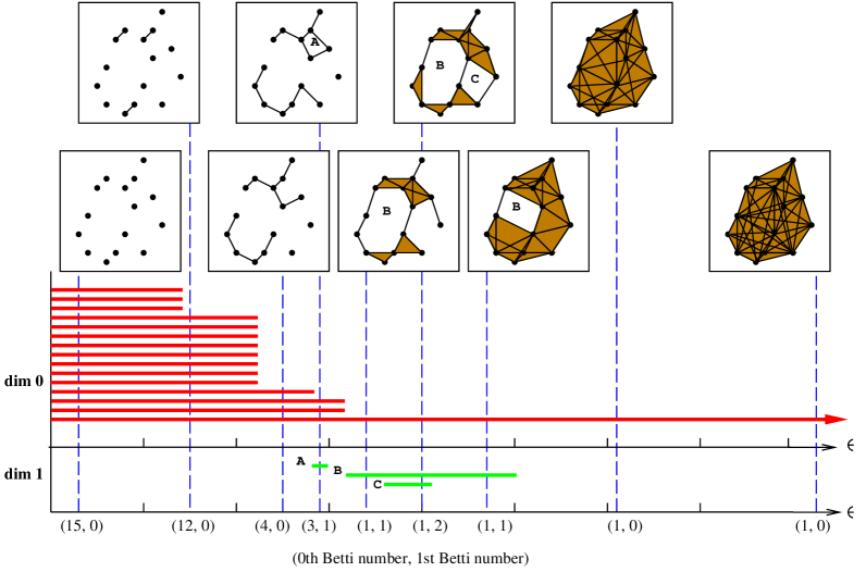
Figure 1: An example of zero- and one-dimensional barcodes for a sequence of Vietoris-Rips complexes

Homology is a tool in algebraic topology used to analyze the connectivity of simplicial complexes, such as points, edges, solid triangles, solid tetrahedra, and other higher dimensional shapes. By using homology, we can measure several features of the data in metric spaces – including the numbers of connected components (0-cycles), holes (1-cycles), voids (2-cycles), etc. We limit the scope of this project to the homology of filtered Vietoris-Rips complexes only.

2.1 Homological Persistence

To construct a filtered Vietoris-Rips complex, a distance threshold $\epsilon$ is chosen first. Then, any two points that are less than the distance $\epsilon$ from each other are connected by an edge. A solid triangle is created if all its three edges have been generated. A solid tetrahedra is constructed if all its face triangles have been created. Similar constructions are used to build higher-dimensional simplices.

Note that different distance thresholds will generate different Vietoris-Rips complexes, and may therefore result in very different homologies, i.e different numbers and types of cycles. Because cycles are the topologically significant features to be captured from the data set, we do not want to miss any of them. For solving this problem, a method, which is called persistent homology ³, is to generate Vietoris-Rips complexes from a set of points at every distance threshold and then derive when the cycles appear and disappear in the complexes as the distance threshold increases. Therefore, the distance threshold is often referred to as time.

The topological data produced by using persistent homology can be visualized through a barcode ²⁵. A barcode is a collection of intervals, where each interval represents a homology class that exists in at least one Vietoris-Rips complex generated from a point cloud. The left and the right endpoint of an interval represents the birth and the death times of a class, respectively. The horizontal axis corresponds to the distance threshold and the vertical axis represents an arbitrary ordering of captured classes.

Figure 1 illustrates an example of zero- and one-dimensional barcodes for a sequence of Vietoris-Rips complexes. The red bars represent the lifetime of the connected components. Note that in the beginning the number of components is the same as the number of points. When the distance threshold $\epsilon$ increases, the number of components is decreased because more and more components are connected together. The green bars represent the lifespans of the cycles in dimension 1. A cycle disappears when it is completely filled in by solid triangles. It can be observed that one cycle, denoted as B in the diagram, is significantly longer than the others, while the cycle A is relatively short-lived. Short-lived cycles are often regarded as “noise,” and long-lived cycles as “true signal,” though these interpretations are subjective in nature and their fitness depends heavily on context. A barcode also encodes all the information regarding the Betti numbers on different scales. Betti numbers count topological features, like connected components (0th Betti number), holes (1st Betti number), voids (2nd Betti number), etc., for an individual simplicial complex. The Betti numbers of the Vietori-Rips complex with distance threshold $\epsilon$ can be found by counting the number of intersections between the barcode and the vertical line the passes through $\epsilon$ on the $x$ axis. The 0th and 1st Betti numbers for several different choices of $\epsilon$ appear along the $x$-axis in Figure 1.

For the computation of persistent homology, there are several open-source software packages available, such as javaPlex ²⁶, Dionysus ²⁷, Perseus ²⁸, Ripser ²⁹, and several others ^{30, 31, 32, 33, 34, 35, 36, 37, 38, 39, 40, 41, 42}. Understanding the performance of persistence solvers is a famously complicated problem. Many elements add to this challenge, but a key contributor is the tremendous variability to be found in size, complexity, and formatting of the data passed as input. A good discussion of the benchmarking problem, and of cross-input variation, may be found in ¹⁶, which reports experimental results for several leading solvers across a variety data sets. By any measure, however, the Eirene library outperforms existing packages by orders of magnitude in both time and memory on certain classes of interest ⁴³, and provides a greater level of detail concerning the relationship between inputs and barcodes than is standard among persistence solvers ⁴⁴.

Libraries of this type generally begin by constructing a filtered simplicial complex from a point cloud and storing the information in a matrix. They next apply matrix reduction techniques and obtains the intervals of the barcode by pairing the simplices in the reduced matrix. As mentioned before, the key feature of Eirene is that it adopts discrete Morse Theory to reduce the matrix size and uses the Schur complement to perform the matrix reduction efficiently.

2.2 Persistence Diagrams

The filtered simplicial complexes constructed to model scientific data are frequently large, with billions and even trillions of component cells. The standard method to compute the persistent homology of a filtered complex $X$ involves a large number of operations on the boundary operator of $X$. The boundary operator is a matrix $D$ whose rows and columns are labeled by the simplices of $X$, and whose entries are determined by a mathematical formula. Constructing and storing boundary matrices for large spaces is computationally expensive. This is the central challenge to high-performance persistent homology solvers.

State of the art platforms circumvent the problem by computing persistence diagrams (equivalently, barcodes) without constructing the full boundary matrix $D$ of $X$, via specialized algorithms, data structures, and mathematical optimizations.

Algorithm 1 Column Algorithm

1:procedure pHcol($D$) $\triangleright$ $D=D_{i=1,\ldots,n}^{j=1,\ldots,n}$ is an $n\times n$ matrix

2:     $R\leftarrow D$, $V\leftarrow I$

3:     for $i=1,\ldots,n$ do

4:         while $\exists j<i$ with $\mathrm{low}_{R}(j)=\mathrm{low}_{R}(i)$ do

5:              $c=R[\mathrm{low}_{R}i,i]/R[\mathrm{low}_{R}j,j]$

6:              $R[...,i]=R[...,i]-cR[...,j]$

7:              $V[...,i]=V[...,i]-cR[...,j]$

8:         end while

9:     end for

10:     $S\leftarrow\{(\mathrm{low}_{R}i,i):R[...,i]\neq 0\}$

11:     return $R,V,S$ $\triangleright$ $R$ is the reduced matrix, $V$ is the column transformation matrix, and $S$ is the set of pivots.

12:end procedure

Algorithm 2 Row Algorithm

1:procedure pHrow($D$) $\triangleright$ $D=D_{i=1,\ldots,n}^{j=1,\ldots,n}$ is an $n\times n$ matrix

2:     $R\leftarrow D$, $V\leftarrow I$

3:     for $i=n$ down to $1$ do

4:         indices = $[j|\mathrm{low}_{R}(j)=i]$

5:         $p$ = indices$[0]$

6:         for $j\in$ indices$[1..]$ do

7:              $c=R[\mathrm{low}_{R}i,i]/R[\mathrm{low}_{R}j,j]$

8:              $R[...,i]=R[...,i]-cR[...,j]$

9:              $V[...,i]=V[...,i]-cR[...,j]$

10:         end for

11:     end for

12:     $S\leftarrow\{(\mathrm{low}_{R}i,i):R[...,i]\neq 0\}$

13:     return $R,V,S$ $\triangleright$ $R$ is the reduced matrix, $V$ is the column transformation matrix, and $S$ is the set of pivots.

14:end procedure

2.2.1 Algorithms

The primary mechanism of most solvers is a matrix decomposition $DV=R$, where $V$ is invertible, upper-triangular, and block-diagonal (blocks correspond to groupings of simplices according to dimension), and $R$ is reduced, in the following sense ^{45, 46}. For any matrix $A$, define $\mathrm{low}_{A}(j)=\mathrm{max}\;\{i:A[i,j]\neq 0\}$. To wit, $\mathrm{low}_{A}(j)$ is the index of the lowest nonzero entry in column $j$. This function is not defined on zero columns. A matrix $R$ is reduced if $\mathrm{low}_{R}$ is injective on its domain of definition. If $t_{j}$ is the time at which simplex $j$ enters the filtration, if every simplex enters at a different time, and if the row and column labels of the boundary matrix $D$ are ordered according to $t$, then for any decomposition $DV=R$ the set

$$\textsc{Pers}(X)=\{(t_{j},t_{\mathrm{low}_{R}(j)}):\mathrm{low}_{R}\textrm{ is defined on $j$}\}$$

is the persistence diagram of the filtered complex. Here $j$ runs over all column-indices in the domain of $\mathrm{low}_{R}$.

Note that the elements of this set are ordered pairs of real numbers. If one regards $(t_{j},t_{\mathrm{low}_{R}(j)})$ not as an ordered pair but as an interval on the real number line, then one obtains the barcode of $X$:

$$\textsc{Barcode}(X)=\{[t_{j},t_{\mathrm{low}_{R}(j)}]\subseteq\mathbb{R}:\mathrm{low}_{R}\textrm{ is defined on $j$}\}$$

Two standard algorithms to compute $V$ and $R$ are Algorithm 1, also called the the column algorithm, and Algorithm 2, also called the row algorithm ⁴⁶.

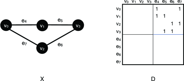
Figure 2: Left A 1-dimensional simplicial complex. Every 1-dimensional simplicial complex is a combinatorial graph. We define a filtration on $X$ by $X_{t}=\{v_{s}:s\leq t\}\cup\{e_{s}:s\leq t\}$. See, for example, Figure 4. Right The boundary matrix of $X$.

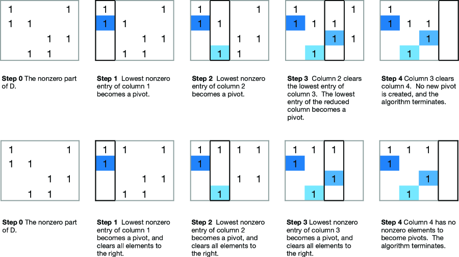
Figure 3: Top row An application of the Column Algorithm to the boundary matrix $D$ in Figure 2. Only the nonzero part of $D$ is shown. Bottom row An application of the Row Algorithm to the the boundary matrix $D$ in Figure 2. Only the nonzero part of $D$ is shown.

Figure 4: The dimension-0 barcode of the filtered complex $X_{t}=\{v_{s}:s\leq t\}\cup\{e_{s}:s\leq t\}$ presented in Figure 2. Dimension-0 homology counts the number of connected components of a space, so the number of bars at time $t$ equals the number of connected components at time $t$. There is one blue bar for each pivot element shown in Figure LABEL:algex_gauss (equivalently, for each pivot element in Figure 4). The birth and death time for each bar may be read from the corresponding pivot. For example, the light blue bar with endpoints $(3,5)$ corresponds to pivot $(v_{3},e_{5})$, located in row 4, column 2 of the reduced boundary matrix. In dimension 0 only, one additional bar must be added, with birth time 0 and death time $\infty$. This is shown in black.

2.2.2 Optimizations and applications of the reported improvements

Several optimizations are available for both Algorithms 1 and 2. Each of those described below offers significant improvements in time and memory. Those employed by Eirene are specially marked.

General optimizations

• Morse reduction (Eirene) A preprocessing step motivated by smooth geometry, which reduces the size of $D$ before it is passed to Algorithm 1 or 2. This is one of the principle methods employed by the software package Perseus ²⁸. Eirene applies a specialized form of Morse reduction which has been observed empirically to reduce the size of the boundary operator by multiple orders of magnitude ¹⁹.

• Clear and compress (Eirene) A preprocessing step motivated by homological algebra, which reduces the size of $D$ before it is passed to either Pers or LU. This method is employed in the platform PHAT ^{31, 47}.

• Data structures Algorithms 1 and 2 depend heavily on efficient look-up of the lowest nonzero entry in each column. Moreover, the columns of $D$ that are eventually cleared play a very minor role. For this reason, it has been found advantageous to store boundary matrices in compressed formats which can be queried for specific column/row information. PHAT, for example, stores sparse columns as heaps, which facilitate efficient queries to $\mathrm{low}_{R}$. Simplex trees and combinatorial number systems have likewise been applied to reduce the cost of storing and manipulating the boundary matrix, e.g. in GUDHI.

• (Re)construction on the fly On the extreme end of compression schemes, it is possible to avoid the construction of $D$ altogether. In this strategy, one does not construct column $j$ of the boundary matrix $D$ until iteration $j$. One then reconstructs the preceding pivot columns as needed to reduce $j$. This method is implemented in the software platform Ripser, and has achieved remarkable performance improvements.

Optimizations for persistence diagrams only

• Persistent cohomology If one wishes to compute persistence diagrams only, and no cycle representatives, then there exists a powerful optimization called persistent cohomology. This method was enabled by a mathematical insight of Cohen-Steiner et al. ⁴⁵, and was concretely described and implemented by Morozov et al. ⁴⁶. These researchers showed that Algorithms 1 and 2 will return the proper pivot elements for a matrix $M$ if they are passed the antitranspose of $M$. For most scientific data sets, it has been observed empirically that (when paired with clear and compress optimization) the time and memory performance of both algorithms improves by several orders magnitude when the anti-transpose is passed, rather than the original input. We are not aware of any theoretical guarantees for this performance increase, as asymptotic behavior on scientific data is extraordinarily difficult to analyze. The phenomenon is very robust in practice, however. See for example ⁴⁶.

Optimizations special to Algorithm 2

Remark 2.1.

These optimizations are used by Eirene, but they can be applied to any implementation of Algorithm 2.

1. Block Reduction (Eirene) This method applies the mathematics of algebraic Morse theory to consolidate the clearing operations of many pivots simultaneously – in effect, block clearing operations. The matrices produced by such operations can be expressed in terms of Schur complements. The calculation of Schur complements involves matrix inversion, multiplication, and addition – these are the operations that are improved by the optimization described in §4.6 below.

2. Dynamic reordering of rows and columns (Eirene) The birth time of simplices does not determine a total ordering on the rows and columns of $D$ in general; this is because many simplices in the same complex may have identical birth times. It has been observed that the choice of row and column order dramatically impacts matrix fill from clearing operations ¹⁹. Moreover, improved row and column orders may be deduced from the structure of the boundary matrix as an increasing number of operations are performed. Thus Eirene dynamically reorders rows and columns following each column reduction. These reordering operations were improved by the optimization of sorting functions described in §4.3.

3. Specialized Vector Fields (Eirene) A critical component of the algorithms employed by Eirene to reorder rows and columns is the calculation of Morse vector fields. These are mathematical objects which, in the current context, are entirely determined by the linear order of rows and columns in the distance matrix $M$. Strategic reordering of the rows/columns of $M$ has been shown to produce much improved vector fields, and the calculation of “good” permutations on $M$ is a second major application of the improved sorting algorithms discussed in §4.3.

2.3 Persistent Generators: The Novel Contribution of Eirene

A set of generators in persistent homology is a collection of cycle representatives (formally, linear combinations of simplices) that parametrize or “generate” the bars of the barcode. Generators in persistent homology may be obtained in several ways. Cohen-Steiner et al. ⁴⁵ showed that generators may be obtained from the columns of the matrix $V$ in the matrix decomposition $D=RV$.

A fundamental obstacle to efficient generator calculation is the sparcity structure of $V$. In scientific applications the superdiagonal blocks of $D$ are short and wide, with columns outnumbering rows by several orders of magnitude. This means that at least one nonzero block of matrix $V$ is large – so large as to be impractical to store or manipulate, even for mesoscale data sets.

The cohomology algorithm circumvents this problem by sacrificing the ability to obtain generators. It applies Algorithm 2 to the antitranpose $D^{\perp}$. The $V$ of this decomposition has much smaller blocks, on the whole, and therefore vastly less scope for fill. However, the $V$ from this decomposition does not provide generators.

With the exception of Eirene, every state of the art persistence solver relies on an variant of the cohomology algorithm to obtain competitive performance results. The time and memory cost to compute generators on cohomology-based platforms is generally several orders of magnitude greater than that needed to compute barcodes. At the current time, Eirene is the only platform capable of computing homological generators within an order of magnitude of the best recorded cost to compute barcodes. This is important, as the computation of generators is fundamentally different to, and strictly harder than, that of barcodes.

A survey of available platforms and run times for barcode computation – without generators – was recently released in ¹⁶. The primary findings of this survey and comparison run times of Eirene are available in ¹⁹. The fundamental insight of Eirene is a combinatorial, matroid-theoretic interpretation of persistence calculation which (a) admits calculation of generators by elementary matrix operations, and (b) reduces fill in the matrix $D$ during reduction ¹⁹.

3 WorldMap: an Example of using Eirene

In this section, we demonstrate an example of how to use Eirene to load data, compute the persistent homology classes, and plot the results graphically. The basic syntax of Eirene is a call to the ezread() function:

     julia> C = eirene(x, keywords ...)where $x$ is either a point cloud encoded as the rows or columns of an array, or a square symmetric matrix (typically a pairwise distance matrix). Keyword arguments specify how this input matrix should be interpreted and processed, and what topological features should be extracted (e.g. homology groups in the first 5 dimensions). The package computes this information and stores the output in a dictionary object C. This object can then be queried for specific information, e.g. Betti curves, or passed to specialized functions for 3D plotting, c.f. Figures 6 and 6.

For a concrete example, suppose we want to explore world geography vis-a-vis networks of neighboring cities. There is a wealth of data available online, and for this demo example we use a catalog of 7322 cities which can be found on the web site simplemaps.com. After downloading the .csv data file, start running a Julia REPL(Read-Evaluate-Print-Loop) to include the Eirene code and then load the data into a 2-dimensional array using the Eirene ezread() wrapper, as shown below.

     julia> include("<file_path_to_Eirene>")     julia> a = ezread("<file_path_to_csv_file>")     7323x9 Array{Any,2}:     "city"          "city_ascii"    "lat"   "lng" ... "country"     "iso2" "iso3" "province"     "Qal eh-ye Now" "Qal eh-ye"     34.983  63.1333   "Afghanistan" "AF"   "AFG"  "Badghis"     "Chaghcharan"   "Chaghcharan"   34.5167 65.25     "Afghanistan" "AF"   "AFG"  "Ghor"     "Lashkar Gah"   "Lashkar Gah"   31.583  64.36     "Afghanistan" "AF"   "AFG"  "Hilmand"     "Zaranj"        "Zaranj"        31.112  61.887    "Afghanistan" "AF"   "AFG"  "Nimroz"     ...

Then, we can extract the spherical coordinates, i.e., columns 3 and 4, from the array a and invoke the function convert() to convert the data type from Any to Float64. Note that Eirene has a built-in function latlon2euc() which can be used to translate spherical coordinates (in degrees, with fixed radius 1) to 3D Euclidean coordinates. The rowsare keyword argument determines wether rows are treated as points or dimensions.

     julia> b = a[2:end,3:4]     7322x2 Array{Any,2}:       34.983   63.1333       34.5167  65.25       31.583   64.36       ...     julia> b = convert(Array{Float64,2},b)     7322x2 Array{Float64,2}:       34.983   63.1333       34.5167  65.25       31.583   64.36       ...     julia> c = latlon2euc(b,rowsare="points")     3x7322 Array{Float64,2}:     0.370265  0.344959  0.368622  0.403432  0.344318  ...  0.81567    0.824296     0.730885  0.748275  0.767998  0.755149  0.768533  ...  0.490971   0.449048     0.573333  0.566646  0.523733  0.516713  0.53926   ... -0.305991  -0.344807

To pass city names to the Eirene function, we need to extract the column 2 of array a. Due to potential errors resulting from nonstandard character strings, it’s good practice to use the built-in label sanitzer ezlabel() to clean this column before assigning to the array d. The wrapper will replace any element of the column that cannot be expressed as an ASCII String with the number corresponding to its row.

     julia> d = ezlabel(a[2:end,2])     7322-element Array{Any,1}:     "Qal eh-ye"     "Chaghcharan"     "Lashkar Gah"     ...With our inputs in order, it’s time to call the main function eirene(). A cursory inspection shows that a number of interesting features appear at or below distance threshold $\epsilon=0.15$ (i.e. approximate to 0.15 * earth radius = 956Km), so we’ll use that as our initial cutoff. As always, the first argument is the most important: this is the matrix c, from which the software will build a reduced Vietoris-Rips complex (this construction is described in §2.1). Keyword rowsare = ‘‘dimensions’’ declares that the rows of c should be regarded as dimensions in Euclidean space, and, conversely, that the columns of c should be regarded as the vertices or 0-simplices in the Vietoris-Rips construction. The properties of this complex computed by Eirene will be stored in a dictionary object $C$, which can be queried with various specialized functions.

     julia> C = eirene(c,rowsare = "dimensions",upperlim = 0.15,pointlabels=d)     elapsed time: 74.892521378 seconds     Dict{ASCIIString,Any} with 14 entries:       "symmat"               => 7322x7322 Array{Int64,2}:       "filtration"           => Any[[515055,515055,515055,515055,515055 ...       ...

Because we did not specify the bettimax parameter when calling the eirene() function, the default is to compute the persistence modules in dimensions 0 and 1. We can use the function plotpersistencediagram_pjs() to view the persistence diagram, as shown in Figure 6. Note that the persistence diagram is an alternative graphical way to represent barcodes. That is, the x-coordinate and the y-coordinate in a persistence diagram represent the birth and death times, respectively. Bars of infinite length appear in red at the point on the diagonal corresponding to the time of their birth. Hovering over a point in the diagram will display the identification number of the corresponding persistent homology class, together with the size the cycle representative Eirene computed for it. To view a specific cycle, we can invoke the function plotclassrep_pjs() by passing the identification number of the class as a parameter.

     julia> plotpersistencediagram_pjs(C)     julia> plotclassrep_pjs(C,class = 1757)

Figure 6 is a 3D visualization of the persistent 1-cycle with the class id number 1757, generated from WorldMap data regarding cities embedded in the Eurasian continent: the Himalayan branch of the silk road is clearly visible on its South West arc; to the North it follows the Trans-Siberian railroad from Moscow in the west to Vladivostok on the Sea of Japan, by way of Omsk, Irktsk, and Chita; from there, it follows the connecting route from Beijing to Hong Kong, passing Nanning, Hanoi, and close to Ho Chi Min on its way to Bangkok (not all of these appear in the cycle itself, but they are easily spotted nearby). With a little exploration we can find large features formed by the Sahara Desert, Tapajos River, Falkland Islands, South China Sea, Guam, and Hudson Bay, and smaller ones shaped by the Andes mountains and Gulf of Mexico - all through the proxy of urban development.

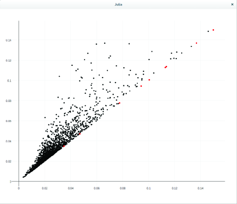
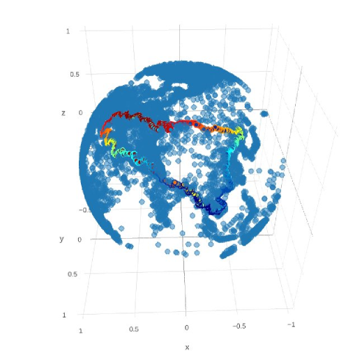
Figure 5: The Persistent Diagram of the WorldMap ($\epsilon=0.15$)

Figure 6: A Cycle in the WorldMap displayed by the Eirene tool

4 Performance-Improving Methods

Code analysis tools are important for programmers to understand program behavior. Software profiling measures the time and memory used during the execution of a program to gain this understanding and thus helps in optimizing code. To develop efficient software, it is essential to identify the major bottlenecks and focus optimization efforts on these. Therefore, our strategy is to use Julia’s built-in Profile module, a statistical profiler, to find the key bottlenecks in Eirene and develop different performance-improving methods to solve them.

To profile an execution of Eirene, we simply need to put the macro @profile before calling the main function of Eirene, e.g.
    @profile C = eirene(data-file-path,...)
Note that the Julia profiling tool works by periodically taking a backtrace during the execution of a program. Each backtrace takes a snapshot of the current state of execution, i.e. the current running function and line number along with the complete chain of function calls which led to this line. Therefore, a busy line of code, such as the code inside nested loops, has a higher likelihood to be sampled and hence appears more frequently in the set of all backtraces. However, profiling a very long-running task may cause the backtrace buffer to fill. Programmers can use the configuration function Profile.init(n, delay) to either increase the total number of backtrace instruction pointers n (default: $10^{6}$) or the sampling interval delay (default: $10^{-3}$) or both.

We used three benchmarks: HIV, WorldMap, and Dragon2, to locate the bottlenecks in Eirene. The HIV benchmark contains the Hamming distances between 1088 different genomic sequence of the HIV virus. The WorldMap benchmark includes the data of 7322 cities in the world. The Dragon2 data set contains 2000 points sampled from the Stanford Dragon graphic. Both of the HIV and the Dragon2 benchmarks are available from ¹⁶, while the WorldMap data can be obtained from ¹⁷.

After the major bottlenecks were identified, we figured out how each was formed and developed targeted solutions, as described below.

4.1 Organization

Recall from §2.2 and §2.3 that Eirene executes a variant of Algorithm 2. Rather than performing row-clearing operations one at a time, this variant eliminates multiple rows in a single pass, via block clearing operations. The primary input to the software is an $m\times m$ distance matrix $S$. The distance matrix mathematically determines an $n\times n$ filtered boundary operator $D$. In general, $n$ is many orders of magnitude larger than $m$. Pseudocode for the work flow appears in Algorithm 3.

Algorithm 3 Morse Reduction

1:procedure Eirene($S$) $\triangleright$ $S=S_{i=1,\ldots,m}^{j=1,\ldots,m}$ is an $m\times m$ distance matrix, with boundary operator $D$

2:     Directly construct a submatrix $E$ of the boundary operator $D$. Matrix $E$ contains all data needed to complete the calculation. $D$ is never stored in memory.

3:     while $E^{T}$ has unreduced columns do

4:         Identify a filtration-compatible discrete Morse vector field $M$ (a special type of square, invertible submatrix).

5:         As in Algorithm 2, perform a block pivot on $M$ to clear all entries to the right in $E^{T}$.

6:     end while

7:      return the set of pivots and the row/column operation matrices that realize this reduction. This suffices to calculate a complete set of generators for the filtered complex.

8:end procedure

Our performance-improving methods address five central issues in this work flow: (a) arrays of type Any, (b) redundant calculations, (c) deeply nested loops, (d) sorting large arrays, and (e) sparse matrix multiplication and addition. These improvements impact the following stages of the work flow.

1. Construction of $E$: (a) arrays of type Any, (b) redundant calculations, (c) deeply nested loops
   Efficient construction of $E$ depends on the reordering of large lists of simplices according to various conditions on their geometric properties. We improved performance by modifying the declared types of some arrays, which were employed at this stage, and by eliminating redundant calculations and deeply nested loops.

2. Construction of Morse vector fields: (d) sorting large arrays
   Eirene applies a principled procedure to select vector fields with advantageous properties at each iteration of the while loop. This procedure has been demonstrated empirically to reduce fill in the submatrix $E$. This method requires reordering of the rows and columns of $E$. We improved the performance by implementing a different sorting algorithm on GPU.

3. Block clearing: (e) sparse matrix multiplication and addition
   The block clearing operation performed on each iteration of the while loop in Algorithm 3 is functionally equivalent to computation of the Schur complement of $M$ in $E$. We parallelized this computation with a master/workers model.

The remainder of this section provides a detailed discussion of points (a)-(e).

Remark 4.1.

Every persistent homology solver that operates on the principle of discrete Morse theory follows the work flow laid out in Algorithm 3. Such implementations will necessarily involve similar variable types and operations: permutations determined by geometric features, arrays of arrays, etc. Consequently, improvements (a)-(e) will adapt directly to any such platform. For example, they will apply to any Eirene-like solver implemented in python or C++.

4.2 Arrays of type Any

Julia’s sampling profiler displays results in textual format only. For faster comprehension, we used the ProfileView package’s function ProfilevView.view(). This function plots a visual representation of the call graph called a flame graph ⁴⁸. The vertical axis of the flame graph (from bottom to top) represents the stack of function calls, while the horizontal axis represents the number of backtraces sampled at each line. To identify a potential bottleneck, the user can hover a cursor over a long bar, usually on the top two levels in the graph, and the corresponding backtrace of the function name and the line number will be shown on the screen.

Figure 7 shows the first performance bottleneck identified, located in the function getstartweights_subr2() using the HIV benchmark. It spans 90% of the horizontal axis and similar results can be found in the other two benchmarks. Examining the code for this function, we found that the use of the array of the abstract-type Any in the following three lines

     val = Array(Any,m)     supp = Array(Any,m)     suppDown = Array(Any,m)

causes the Julia interpreter to generate many dynamic invoker objects when these three arrays appeared in an expression. Performance is greatly suffered as a result. Fortunately, the abstract-type Any is unnecessary in this function because the array supp[] stores only indices (i.e. of integer type) of non-zero elements returned from the Julia function find(). After replacing the abstract-type Any with the static-type Int64, this bottleneck has been solved.

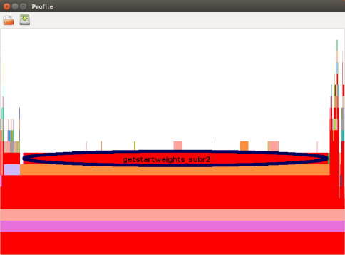
Figure 7: Identification of the bottleneck caused by the array of type Any

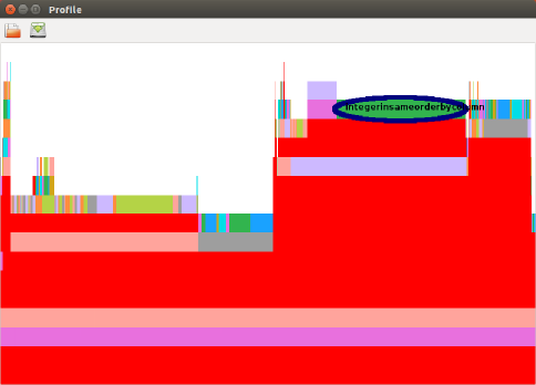
Figure 8: Identification of the bottleneck in the function integersinsameorderbycolumn

4.3 Redundant Calculations

We ran the code and performed the profiling procedure again after fixing the first large bottleneck. We noticed that there is a certain amount of time spent in the function integersinsameorderbycolumn() when running the Dragon2 benchmark, as shown in Figure 8. Further investigation shows that this delay resulted from a number of unnecessary calculations. As shown in the upper box in Figure 9, the array y is used to calculate the prefix sums of the array x, only a fraction of which will be copied to the array z and returned to its caller. When the maxvalue, a parameter passed to this function, is large, the inner loop for i = 1:maxvalue will let this function be executed much longer. As shown in the bottom box in Figure 9, we modified the code to find out the range first and then calculate only the prefix sums within this range. Furthermore, we can just use the array x to accumulate the prefix sums of itself instead of using another local array y. The initialization of the whole array x inside the beginning of the loop (i.e. x[:] = 0) can also be replaced by cleaning up the dirty elements before the end of the loop. Note that a single colon in Julia indicates every row or column.

            ...         for j = 1:numcols                  x[:] = 0                  for i = colptr[j]:(colptr[j+1]-1)                          x[v[i]]+=1                  end                  y[1] = colptr[j]                  for i = 1:maxvalue                          y[i+1]=y[i]+x[i]                  end                  for i = colptr[j]:(colptr[j+1]-1)                          u = v[i]                          z[i] = y[u]                          y[u]+=1                  end          end          return z     

             ...          x[:] = 0          for j = 1:numcols                  for i = colptr[j]:(colptr[j+1]-1)                          x[v[i]]+=1                  end                    maxv = v[colptr[j]];   minv = maxv                  for i = (colptr[j]+1):(colptr[j+1]-1)                      if v[i] > maxv                         maxv = v[i]                      elseif v[i] < minv                         minv = v[i]                      end                  end                    prevsum = colptr[j]                  for i = minv:maxv                          sum = prevsum + x[i]                          x[i] = prevsum                          prevsum = sum                  end                  for i = colptr[j]:(colptr[j+1]-1)                          u = v[i]                          z[i] = x[u]                          x[u]+=1                  end                    for i = minv:maxv                          x[i] = 0                  end          end          return z     

Figure 9: The original(top) and the modified(bottom) function integersinsameorderbycolumn() in Eirene

4.4 Deeply Nested Loops

Even after we removed the overhead caused by the unnecessary array of type Any in the function getstartweights_subr2(), the execution of the Dragon2 benchmark still spends a reasonable amount of time on this function. As shown in Figure 10, this function calculates the weight for each column in the matrix s. It firstly finds the indices of the non-zero elements in each column and then uses nested loops to increment the counter of the column if certain conditions are met. Note that the array base function find(X) in Julia returns a vector of the linear indices of non-zeros in the array X. Hence, the code find(s[:,i]) in Figure 10 will return the row indices of the non-zero elements in the ith column. When there are many non-zero elements in the matrix s, the deeply nested loops will consume much CPU computation time.

     function getstartweights_subr2(s::Array{Int64,2},              w::Array{Int64,1},m::Int64)     ...     for i = 1:m         supp[i] = find(s[:,i])         l[i] = length(supp[i])         ...     end     for i = 1:m         Si = supp[i]         ...         for jp = 1:l[i]             ...             for ...                if conditions met                    w[i]+=1                end             end         end     end  end     

Figure 10: The original function getstartweights_subr2() in Eirene

To deal with the deeply nested loops, one feasible approach is to use the GPU to accelerate the execution. NVIDIA provides a parallel computing platform and programming model called CUDA (Compute Unified Device architecture). Therefore, now it is much more convenient to write application programs on the GPUs for processing large amounts of data, without the need to use low-level assembly language code.

The NVIDIA GPU architecture consists of a scalable number of streaming multiprocessors (SMs), each containing many streaming processors (SPs) or cores to execute the lightweight threads. The kernel function, which is declared by using the __global__ qualifier keyword in front of a function heading, is executed on the GPU device. It consists of a grid of threads and these threads are divided into a set of blocks, each block containing multiple warps of threads. Blocks are distributed evenly to the different SMs to run. A warp, which has 32 consecutive threads bundled together, is executed using the Single Instruction, Multiple Threads (SIMT) style. Note that the GPU device has its own off-chip device memory (i.e. global memory) and on-chip faster memory such as registers and shared memory. Fancy warp shuffle functions are also supported in modern GPUs⁴⁹. They permit exchanging of variables (i.e. registers) between threads within a warp without using shared memory.

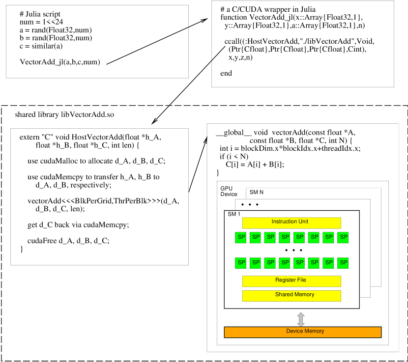
Figure 11: An example of calling C/CUDA functions from a Julia script

Though there are some Julia packages which enable programmers to launch GPU kernel calls, we decided to implement our own wrappers for greater flexibility and efficiency. Figure 11 shows an example of calling a CUDA function named vectorAdd() by way of the host function HostVectorAdd() in C. A wrapper function in Julia is needed, which utilizes the ccall() function to invoke the host function. Note that the first argument of ccall() is a tuple pair (:function,"library-path"). The rest of the arguments include the function return type, a tuple of input parameter types, and then the actual parameters. The C/CUDA functions should be compiled and linked as a shared objects. It is worth mentioning that, when using the nvcc NVIDIA CUDA Compiler to compile the C/CUDA code, programmers need to use the options -Xcompiler -fPIC to pass the position-independent code (PIC) option from nvcc to g++.

     _global__ void init_supp(const long long *s, int *supp, int *l, ..., long long m) {     int tid = blockIdx.x * blockDim.x + threadIdx.x;     int lnid = threadIdx.x % WARP_SIZE ; // lane id     int warp_id = tid >> 5; // global warp number     if(warp_id >= m) return;       int supplen = 0;     int j = lnid;       while (j < m ) {        int b = s[warp_id*m + j] != 0 ;        int votes = __ballot( b ); // cast b if non-zero        int lidx = __popc( votes & ((1 << lnid) - 1)) ;          if (b)          supp[warp_id*m + supplen+lidx] = j;          supplen += __popc(votes);        j += WARP_SIZE; // next stride     }     ...     if(lnid == 0) {        l[warp_id] = supplen;         ...     }  }    _global__ void calcstartweights(const long long *s, int *supp, int *l, long long *w, long long m) {   // Same as in init_supp, calc. tid , lnid, and warp_id ;     if(warp_id >= m) return;       int supplen = l[warp_id];     int jp = lnid;     int wt = 0; // each thread has a counter (in register)     while (jp < supplen) {        int j = supp[warp_id*m  + jp];         ...             for ... {                 if ( conditions met )                   wt += 1;             }        jp += WARP_SIZE; // next stride     }     // parallel reduction sum through registers     for(int offset = WARP_SIZE>>1; offset>0; offset >>= 1)         wt += __shfl_down(wt, offset);       if (lnid == 0) w[warp_id] = wt;  }    extern "C" void Host_getstarweights(long long * s, long long *h_w , long long m) {     use cudaMalloc to allocate d_s, d_supp, d_l, d_w, etc.       use cudaMemcpy to transfer data to d_s on GPU       init_supp<<<BlkPerGrid, ThrPerBlk>>>(d_s, d_supp, d_l,..., m);       calcstartweights<<<BlkPerGrid, ThrPerBlk>>>(d_s, d_supp, d_l, d_w, m);       use cudaMemcpy to get the weights h_w from device d_w  }     

Figure 12: Implementation of the getstartweights_subr2() on GPU

Figure 12 shows our implementation of the function getstartweights_subr2(). Our idea is to use m warps to handle the outermost for i=1:m loop in the original code. Since the second for i=1:m loop needs the result from the first loop, we need to use two kernel functions: init_supp() and calcstartweights(), and launch them one after the other in the host function Host_getstarweights(). To find the indices of the non-zero elements for each column, each thread within a warp checks the corresponding element and casts its one-bit vote via the __ballot() intrinsic function. The __ballot() collects the votes from all threads in a warp into a 32-bit integer and returns this integer to every thread. The __popc(int v) function returns the number of bits which are set to 1 in the 32-bit integer v. That is, it performs the population count operation. By combining the __ballot() and __popc() functions along with bit-masking, each thread in a warp can quickly find out how many non-zero elements are in front of it, and then store its index into the corresponding location in the array supp[]. This procedure will be repeated stride by stride until all elements in a column have been processed. Note that similar strategies have been used in ⁵⁰ and ⁵¹ to perform efficient stream compactions on GPU.

After determining the indices of the non-zero elements for each column, each thread in the second kernel function calcstartweights() uses a local counter (i.e. a register) and increments this counter by one if certain conditions are met. When all non-zero elements have been checked, a parallel reduction sum operation via the efficient shuffle function __shfl_down() is performed. All of the local counter values in each warp will be added together and stored into the counter at the first thread (i.e lane ID 0). This thread then writes the weight to the output array w.

4.5 Sortperm a Large Array

Another bottleneck occurs in the function ordercanonicalform() when it calls Julia’s steeper(v) to find the rank of each element in the distance matrix. The sortperm(v) computes a permutation of the array v’s indices that puts the array into sorted order. For example, if the input array v is
      v = [ 7, 3, 8, 4, 2 ] ,
then the output from sortperm(v) will be
      [ 5, 2, 4, 1, 3 ] .
When the size of the matrix is large, e.g. the WorldMap benchmark, sortperm(v) performs poorly. We found out that if we change the default sorting algorithm from MergeSort to RadixSort, the performance can be greatly improved, especially for the WorldMap benchmark.

Furthermore, CUDA Thrust is a powerful library⁵² which provides a rich collection of data parallel primitives such as sort, scan, reduction, etc. Hence, using CUDA Thrust to build GPU applications, programming efforts can be reduced greatly. Though CUDA Thrust does not support the sortperm-like function directly, we can simply use the sequence() and sort_by_key() to implement it on GPU quickly, as shown in Figure 13.

     extern "C" void  sortperm_thrust(double *h_s, long long *h_idx, long long n)  {     thrust::device_ptr<long long> d_idx =                       thrust::device_malloc<long long>(n);     // create an array with elements 1, 2, 3, ..., n     thrust::sequence(d_idx, d_idx + n, 1);       thrust::device_ptr<double> d_s =                       thrust::device_malloc<double>(n);       thrust::copy(h_s, h_s+n, d_s); // copy s to device       thrust::sort_by_key(d_s, d_s + n, d_idx);       // we are interested in idx     thrust::copy(d_idx, d_idx + n, h_idx);       thrust::device_free(d_s);     thrust::device_free(d_idx);  }     

Figure 13: Implementation of sortperm() on GPU

4.6 Sparse Matrix Multiplication and Addition

For efficiently computing the matrix reduction, the Eirene library uses the Schur complement to encapsulate the LU factorization ¹⁹. Given a matrix M with submatrices A, B, C, and D as shown below,

$$M=\begin{bmatrix}A&B\\ C&D\end{bmatrix}$$

the Schur complement S of the block A is

$$S=D+CA^{-1}B$$

using the modulo-2 operation. Inside the Schur complement function schurit4!() in Eirene, the function blockprodsum() is invoked to compute $D+CE$ after getting $E=A^{-1}B$. Though Eirene uses sparse matrices for computing, we found that the function blockprodsum() becomes a bottleneck for large arrays.

To alleviate this problem, we decided to take the advantage of the multicore architecture and adopted the master/workers parallel computation model to speed up the execution. We partitioned the matrices D and E columnwise (due to the use of Compressed Sparse Column(CSC) format in Eirene) into several workers (i.e. pthreads) and let each worker $i$ compute $S_{i}=D_{i}+CE_{i}$, as illustrated in Figure 14. Unlike the dense matrix multiplication in which the product matrix is fully data parallel after partitioned, the index pointers in CSC which point to the starting locations of every column have to be adjusted one after the other. We let the master do the adjusting work when it copies the result to its caller.

Figure 14: Parallel Implementation of blockprodsum() using Master/Workers

5 Experimental Results

To evaluate the effects of the performance-improving methods discussed in the previous section, we ran experiments with three different versions of Eirene: the original version which is Eirene v0.3.5 released in January 2017; the modified version which removes the unnecessary array of type Any, avoids unnecessary calculations, and uses RadixSort in sortperm(); the enhanced version which is a superset of the modified version and utilizes manycore/multicore to calculate the getstartweights_subr2(), sortperm(), and the blockprodsum() (using 4 workers).

We firstly adopted the workstation at the Ohio Supercomputing Center(OSC) to conduct the experiments. The machine has the Intel Xeon E5-2680 v4 CPU (2.4GHz), 28 cores per node, 128 GB of memory, as well as a cutting-edge NVIDIA Pascal P100 GPU(1.33GHz, 3584 CUDA cores, 16GB) running CUDA Driver Version 8.0. Tables  1, 2, and  3 show execution times for the major bottlenecks and the total execution time for the HIV, WorldMap and Dragon2 benchmarks, respectively. In these three tables, we use A, B, C, D, and E to denote the major bottlenecks caused by abstract-type "Any" , integersinsameorderbycolumn(), getstartweights_subr2(), sortperm(), and blockprodsum().

Table 1: Execution Times (in seconds) of the Major Bottlenecks using the HIV Benchmark                                                                                                                                    (Intel Xeon E5-2680 v4 and NVIDIA Tesla P100 (Pascal))

	Original	Modified	Enhanced
A	95.7	0	0
B	0.078	0.002	0.002
C	3.2	3.2	0.068(Manycore)
D	0.42	0.043(RadixSort)	0.008(Manycore)
E	0.135	0.135	0.134(Multicore)
Total	110.8	13.1	9.9

Table 2: Execution Times (in seconds) of the Major Bottlenecks using the WorldMap Benchmark                                                                                                                                    (Intel Xeon E5-2680 v4 and NVIDIA Tesla P100 (Pascal))

	Original	Modified	Enhanced
A	18.6	0	0
B	2.2	0.002	0.002
C	1.3	1.3	0.29(Manycore)
D	38.8	4.1 (RadixSort)	0.39(Manycore)
E	1.18	1.18	0.90(Multicore)
Total	80.6	23.4	17.1

Table 3: Execution Times (in seconds) of the Major Bottlenecks using the Dragon2 Benchmark                                                                                                                                    (Intel Xeon E5-2680 v4 and NVIDIA Tesla P100 (Pascal))

	Original	Modified	Enhanced
A	416.6	0	0
B	36.2	0.05	0.05
C	15.4	15.4	0.72(Manycore)
D	2.4	0.41(RadixSort)	0.03(Manycore)
E	15.5	15.5	9.6(Multicore)
Total	565.2	109.9	89.0

It can be seen that the removal of unnecessary use of the array of type Any can greatly improve the performance for all benchmarks. The other methods also have positive impacts on the performance for different benchmarks. Note that there is no significant improvement for the HIV and Worldmap benchmarks when using multicore to speed up the blockprodsum() due to the small amount of computation. However, we used different number of threads to compute the blockprodsum() for the Dragon2 benchmark. As shown in Table 4, using a few more threads can still improve the performance. For parallel dense matrix multiplication, usually linear or close to linear speedups can be obtained. The reason we cannot get linear speedups here is because the matrices are sparse and the workload is not fully balanced among the worker threads. Currently, a load balancing implementation of the blockprodsum() function is being developed.

Table 4: Execution Times (in seconds) of the blockprodsum() in Dragon2 Benchmark with different number of workers

Num. of Workers	1	2	4	6	8	10	12
Time	15.5	11.3	9.6	9.2	8.6	8.4	8.3

In addition to the three benchmarks mentioned above, we also ran another four benchmarks: Dragon1, C. elegans, Klein_4, and Klein_9, all available from ¹⁶. The Dragon1 is a 1000-point data set sampled from the Stanford Dragon graphic, the C. elegans benchmark is a neuronal network with 297 neurons, while Klein 400 and Klein 900 are the data sets sampled from the Klein bottle pictures with 400 and 900 points, respectively. Except the WorldMap benchmark which sets epsilon = 0.15, all benchmarks use Eirene’s default setting Inf as the max distance threshold. Table 5 shows the timing results on a workstation at OSC. To show our methods can also work well on different hardware platforms, we ran the benchmarks using the workstation in our laboratory. Table 6 displays the results from a workstation with Intel Xeon CPU E3-1231(3.40GHz, 8GB memory) and NVIDIA Quadro K620 (Maxwell) GPU. This machine has higher CPU clock rate but older GPU model than the OSC workstation.

Table 5: Execution Times (in seconds) of the Benchmarks using Intel Xeon E5-2680 v4 and NVIDIA Tesla P100 (Pascal)

Name (Size of complex)	Original	Modified	Enhanced
C. elegans ($4.4\times 10^{6}$)	4.9	2.2	1.9
Klein 400 ($1.1\times 10^{7}$)	7.4	2.7	2.3
Klein 900 ($1.2\times 10^{8}$)	61.9	10.3	9.8
HIV ($2.1\times 10^{8}$)	110.8	13.1	9.9
Dragon1 ($1.7\times 10^{8}$)	57.3	12.8	11.2
Dragon2 ($1.3\times 10^{9}$)	565.2	109.9	89.0
WorldMap ($2.0\times 10^{8}$)	80.6	23.4	17.1

Table 6: Execution Times (in seconds) of the Benchmarks using Intel Xeon E3-1231 and NVIDIA Quadro K620 (Maxwell)

Name (Size of complex)	Original	Modified	Enhanced
C. elegans ($4.4\times 10^{6}$)	4.7	2.2	2.1
Klein 400 ($1.1\times 10^{7}$)	7.3	2.6	2.5
Klein 900 ($1.2\times 10^{8}$)	58.2	11.5	10.1
HIV ($2.1\times 10^{8}$)	108.4	13.0	11.1
Dragon1 ($1.7\times 10^{8}$)	54.1	12.4	11.7
Dragon2 ($1.3\times 10^{9}$)	543.0	110.3	94.0
WorldMap ($2.0\times 10^{8}$)	74.9	23.1	17.9

We also measured the memory usage(in GB) of each benchmark on two different hardware platforms. We found that the memory usage stays constant on different machines, due to the same software (i.e. Julia) version and configuration. Therefore, we only present one set of data in Table7 which shows the size of memory used by each benchmark under different implementations of Eirene. It can be observed that the original version of Eirene used much more memory because it used the array of the abstract-type Any. The enhanced version used a little more memory than the modified version due to some memory allocated in the wrapper functions.

Table 7: Memory Usage (in GB) for each version of the Benchmarks on three Different Hardware Platforms             

Name (Size of complex)	Original	Modified	Enhanced
C. elegans ($4.4\times 10^{6}$)	1.30	0.61	3.96
Klein 400 ($1.1\times 10^{7}$)	2.43	1.07	4.43
Klein 900 ($1.2\times 10^{8}$)	28.91	7.23	13.80
HIV ($2.1\times 10^{8}$)	43.55	9.75	13.02
Dragon1 ($1.7\times 10^{8}$)	24.80	6.94	11.30
Dragon2 ($1.3\times 10^{9}$)	262.59	51.02	56.91
WorldMap ($2.0\times 10^{8}$)	22.99	15.88	21.96

6 Conclusion

We used the profiling tools in Julia to identify the bottlenecks in Eirene, an open-source platform for computing persistent homology. Several performance-improving methods targeting the bottlenecks have been developed, such as removing unnecessary use of the array of the abstract-type Any, eliminating redundant computation, use of manycore/multicore to accelerate execution, etc. Experimental results demonstrate that the performance can be greatly improved.

References

- 1 Frosini P. Measuring Shape by Size Functions. In: Proceedings of SPIE on Intelligent Robotic Systems:122–133; 1991.
- 2 Robins V. Towards computing homology from finite approximations. In: Proceedings of the 14th Summer Conference on General Topology and its Applications (Brookville, NY, 1999):503–532; 1999.
- 3 Edelsbrunner H, Letscher D, Zomorodian A. Topological Persistence and Simplification. Discrete & Computational Geometry. 2002;28(4):511–533.
- 4 Zomorodian A, Carlsson G. Computing persistent homology. Discrete Comput. Geom.. 2005;33(2):249–274.
- 5 Chazal F, Cohen-Steiner D, Glisse M, Guibas L. J, Oudot S. Y. Proximity of Persistence Modules and Their Diagrams. In: Proceedings of the Twenty-fifth Annual Symposium on Computational GeometrySCG ’09:237–246ACM; 2009; New York, NY, USA.
- 6 Cohen-Steiner D, Edelsbrunner H, Harer J. Stability of Persistence Diagrams. Discrete & Computational Geometry. 2007;37(1):103–120.
- 7 Lesnick M. The Optimality of the Interleaving Distance on Multidimensional Persistence Modules. 2011;.
- 8 Carlsson G. Topology and data. Bull. Amer. Math. Soc. (N.S.). 2009;46(2):255–308.
- 9 Ghrist R. Barcodes: the persistent topology of data. Bull. Amer. Math. Soc. (N.S.). 2008;45(1):61–75.
- 10 Edelsbrunner H, Morozov D. Persistent Homology: Theory and Practice. In: European Congress of Mathematics:31–50European Mathematical Society; 2012.
- 11 Giusti C, Ghrist R, Bassett D. S. Two’s company, three (or more) is a simplex. Journal of Computational Neuroscience. 2016;41(1):1–14.
- 12 Chan J. M, Carlsson G, Rabadan R. Topology of viral evolution. In: Proceedings of the National Academy of Sciences of the United States of America, vol. 110: ; 2013.
- 13 Carlsson G, T. Ishkhanov V. d. S, Zomorodian A. On the Local Behavior of Spaces of Natural Images. International Journal of Computer Vision. 2008;76:1–12.
- 14 Silva V. D, Ghrist R. Coverage in sensor networks via persistent homology. Algebraic & Geometric Topology. 2007;7:339–358.
- 15 Pranav P, Edelsbrunner H, Weygaert R, et al. The Topology of the Cosmic Web in Terms of Persistent Betti Numbers. Monthly Notices of the Royal Astronomical Society. 2016;465(4):4281–4310.
- 16 Otter N, Porter M, Tillmann U, Grindrod P, Harrington H. A Roadmap for the Computation of Persistent Homology arXiv:1506.08903; .
- 17 Henselman-Petrusek G. Eirene: a platform for computational homological algebra http://gregoryhenselman.org/eirene.html.
- 18 The Julia Language https://julialang.org/.
- 19 Henselman-Petrusek G. Matroids, Filtrations, and Applications PhD thesis, University of Pennsylvania, 2016; .
- 20 Graham S. L, Kessler P. B, McKusick M. K. An execution profiler for modular programs. Software: Practice and Experience. 1983;13(8):671–685.
- 21 McKusick M. K. Using gprof to Tune the 4.2BSD Kernel. In: Proceedings of the European UNIX Users Group Meeting, Nijmegen, Netherlands.; 1984.
- 22 Nichols B, Buttlar D, Farrel J. P. Pthreads Programming. Sebastopol, CA 95472: O’Reilly & Associates, Inc.; first ed.1996.
- 23 Kirk D. B, Hwu W.-m. W. Programming Massively Parallel Processors: A Hands-on Approach. San Francisco, CA, USA: Morgan Kaufmann Publishers Inc.; 3rd ed.2016.
- 24 Hylton A, Henselman-Petrusek G, Sang J, Short R. Performance Enhancement of a Computational Persistent Homology Package. In: Proceedings of IEEE International Performance Computing and Communications Conference; 2017.
- 25 Ghrist R. Barcodes: The persistent topology of data. Bulletin of the American Mathematical Society. 2007;45:61–75.
- 26 Tausz A, Vejdemo-Johansson M, Adams H. JavaPlex: A research software package for persistent (co)homology. In: Proceedings of ICMS 2014Lecture Notes in Computer Science 8592:129-136; 2014.
- 27 Morozov D. Dionysus http://www.mrzv.org/software/dionysus/.
- 28 Nanda V. Perseus, the persistent homology software http://www.sas.upenn.edu/~vnanda/perseus.
- 29 Bauer U. Ripser, Available at: https://github.com/Ripser/ripser .
- 30 Bauer U, Kerber M, Reininghaus J. DIPHA (A distributed persistent homology algorithm). Available at https://code.google.com/p/dipha/ .
- 31 Bauer U, Kerber M, Reininghaus J, Wagner H. PHAT – Persistent Homology Algorithms Toolbox:137–143. Berlin, Heidelberg: Springer Berlin Heidelberg 2014.
- 32 Bubenik P, Dlotko P. A persistence landscapes toolbox for topological statistics. CoRR. 2015;abs/1501.00179.
- 33 Dey T. K, Shi D, Wang Y. SimBa: An Efficient Tool for Approximating Rips-filtration Persistence via Simplicial Batch-collapse. ArXiv e-prints. 2016;.
- 34 Dlotko P. Persistence landscape toolbox. Available at: https://www.math.upenn.edu/ dlotko/persistenceLandscape.html .
- 35 Fasy B, Kim J, Lecci F, Maria C, Rouvreau V. TDA: Statistical tools for topological data analysis. Available at https://cran.r-project.org/web/packages/ TDA/index.html .
- 36 Fasy B. T, Kim J, Lecci F, Maria C. Introduction to the R package TDA. ArXiv e-prints. 2014;.
- 37 Lesnick M, Write M. RIVET: The rank invariant visualization and exploration tool, 2016. Available at http://rivet.online/ .
- 38 Clément M, Boissonnat J.-D, Glisse M, Yvinec M. The Gudhi library: Simplicial complexes and persistent homology. In: International Congress on Mathematical Software:167–174Springer; 2014.
- 39 D. o. C. S. Jyamiti research group (Prof. Tamal K. Dey), O. S. U. Engineering . SimpPers, 2014. Available at http://web.cse.ohio-state.edu/ tamaldey/SimpPers/SimpPers-software/ .
- 40 D. o. C. S. Jyamiti Research Group (Prof. Tamal K. Dey), O. S. U. Engineering . GIComplex, 2013. Available at http://web.cse.ohio-state.edu/ tamaldey/GIC/GICsoftware/ .
- 41 Perry P, Silva V. Plex, 2000–2006. Available at http://mii.stanford.edu/research/comptop/programs/ .
- 42 Tausz A, Vejdemo-Johansson M, Adams H. javaPlex: a research platform for persistent homology. In: Book of Abstracts Minisymposium on Publicly Available Geometric/Topological Software:7; 2012.
- 43 Henselman-Petrusek G. Matroids and Canonical Forms: Theory and Applications. Dissertations available from ProQuest. AAI10277847. 2017;.
- 44 Henselman-Petrusek G, Ghrist R. Matroid Filtrations and Computational Persistent Homology. ArXiv e-prints. 2016;.
- 45 Cohen-Steiner D, Edelsbrunner H, Morozov D. Vines and vineyards by updating persistence in linear time. In: Proceedings of the 22nd annual Symposium on Computational Geometry (SoCG)SCG ’06:119–126ACM; 2006; New York, NY, USA.
- 46 Silva V, Morozov D, Vejdemo-Johansson M. Dualities in persistent (co)homology. Inverse Problems. 2011;27(12):124003, 17.
- 47 Bauer U, Kerber M, Reininghaus J. Clear and compress: computing persistent homology in chunks. In: Topological Methods in Data Analysis and Visualization IIIMathematics and Visualization. 2014 (pp. 103-117).
- 48 Gregg B. The Flame Graph. Communications of the ACM. 2016;59(6):48–57.
- 49 Harris M. CUDA Pro Tip: Do The Kepler Shuffle, PARALLEL FORALL http://devblogs.nvidia.com/parallelforall/cuda-pro-tip-kepler-shuffle/2015.
- 50 Harris M, Garland M. Optimizing Parallel Prefix Operations for the Fermi Architecture. San Francisco, CA, USA: Chapter 3 of the book "GPU Computing Gems - Jade Edition", Morgan Kaufmann Publishers Inc.; 2011.
- 51 Rego V, Sang J, Yu C. A Fast Hybrid Approach for Stream Compaction on GPUs. In: Proceedings of International Workshop on GPU Computing and Applications; 2016.
- 52 Hoberock J, Bell N. Thrust: A parallel algorithms library which resembles the C++ Standard Template Library (STL) http://thrust.github.io2015.