Hybrid matrix compression for high-frequency problems

Abstract

Boundary element methods for the Helmholtz equation lead to large dense matrices that can only be handled if efficient compression techniques are used. Directional compression techniques can reach good compression rates even for high-frequency problems.

Currently there are two approaches to directional compression: analytic methods approximate the kernel function, while algebraic methods approximate submatrices. Analytic methods are quite fast and proven to be robust, while algebraic methods yield significantly better compression rates.

We present a hybrid method that combines the speed and reliability of analytic methods with the good compression rates of algebraic methods.

1 Introduction

We consider the Helmholtz single layer potential operator

$$\mathcal{G}[u](x):=\int_{\Omega}g(x,y)u(y)\,dy,$$

where $\Omega\subseteq\mathbb{R}^{3}$ is a surface and

$$g(x,y)=\frac{\exp(\mathbf{i}\kappa\|x-y\|)}{4\pi\|x-y\|}$$ (1)

denotes the Helmholtz kernel function with the wave number $\kappa\in\mathbb{R}_{\geq 0}$.

Applying a standard Galerkin discretization scheme with a finite element basis $(\varphi_{i})_{i\in\mathcal{I}}$ leads to the stiffness matrix $G\in\mathbb{C}^{\mathcal{I}\times\mathcal{I}}$ given by

$$g_{ij} =\int_{\Omega}\varphi_{i}(x)\int_{\Omega}g(x,y)\varphi_{j}(y)\,dy\,dx \text{ for all }i,j\in\mathcal{I},$$ (2)

where we assume that the basis functions are sufficiently smooth to ensure that the integrals are well-defined even if the supports overlap, e.g., for $i=j$. Due to $g(x,y)\neq 0$ for all $x\neq y$, the matrix $G$ is not sparse and therefore requires special handling if we want to construct an efficient algorithm.

Standard techniques like fast multipole expansions [18, 12], panel clustering [15, 20], or hierarchical matrices [13, 14, 10] rely on local low-rank approximations of the matrix. In the case of the high-frequency Helmholtz equation, e.g., if the product of the wave number $\kappa$ and the mesh width $h$ is bounded, but not particularly small, these techniques can no longer be applied since the local ranks become too large. This situation frequently appears in engineering applications.

The fast multipole method can be generalized to handle this problem by employing a special expansion that leads to operators that can be diagonalized, and therefore evaluated efficiently [19, 11].

The butterfly method (also known as multi-level matrix decomposition algorithms, MLMDA) [17] achieves a similar goal by using permutations and block-diagonal transformations in a pattern closely related to the fast Fourier transformation algorithm.

Directional methods [5, 7, 16, 1] take advantage of the fact that the Helmholtz kernel (1) can be written as a product of a plane wave and a function that is smooth inside a conical domain. Replacing this smooth function by a suitable approximation results in fast summation schemes.

We will focus on directional methods, since they can be applied in a more general setting than the fast multipole expansions based on special functions, and since they offer the chance of achieving better compression to $\mathcal{O}(n\log n)$ coefficients compared to $\mathcal{O}(n\log^{2}n)$ required by the butterfly scheme [17].

In particular, we will work with directional $\mathcal{H}^{2}$-matrices (abbreviated $\mathcal{DH}^{2}$-matrices), the algebraic counterparts of the directional approximation schemes used in [5, 7, 16]. Our starting point is the directional Chebyshev approximation scheme introduced in [16] and analyzed in [4]. While this approach is fast and proven to be reliable, the resulting ranks are quite large, and this leads to unattractive storage requirements.

We can solve this problem by applying an algebraic recompression algorithm that starts with the $\mathcal{DH}^{2}$-matrix constructed by interpolation and uses nested orthogonal projections and singular value decompositions (SVD) to significantly reduce the rank. This algorithm is based on the general $\mathcal{DH}^{2}$-matrix compression algorithm introduced in [3], but takes advantage of the previous approximation in order to significantly reduce the computational work to $\mathcal{O}(nk^{3}\log n)$ in the high-frequency case, cf. Theorem 4.18 and Remark 4.20.

Compared to the closely related algorithm presented in [16], our algorithm compresses the entire $\mathcal{DH}^{2}$-matrix structure instead of just the coupling matrices, and the orthogonal projections applied in the recompression algorithm allow us to obtain straightforward estimates for the compression error.

Compared to the algorithm presented in [1], our approach has better stability properties, owing to the results of [4] for the interpolation scheme and the orthogonal projections employed in [3] for the recompression, and it can be expected to yield better compression rates, since it uses an $\mathcal{H}^{2}$-matrix representation for low-frequency clusters, while the algorithm of [1] relies on the slightly less efficient $\mathcal{H}$-matrices.

2 Directional $\mathcal{H}^{2}$-matrices

Hierarchical matrix methods are based on decompositions of the matrix $G$ into submatrices that can be approximated by factorized low-rank matrices. In our case, we follow the directional interpolation technique described in [16] and translate the resulting compressed representation into an algebraical definition that can be applied in more general situations.

In order to describe the decomposition into submatrices, we first introduce a hierarchy of subsets of the index set $\mathcal{I}$ corresponding to the box trees used, e.g., in fast multipole methods.

Definition 1 (Cluster tree)

Let $\mathcal{T}$ be a labeled tree such that the label $\hat{t}$ of each node $t\in\mathcal{T}$ is a subset of the index set $\mathcal{I}$. We call $\mathcal{T}$ a cluster tree for $\mathcal{I}$ if

• the root $r\in\mathcal{T}$ is labeled $\hat{r}=\mathcal{I}$,

• the index sets of siblings are disjoint, i.e.,

  $$t_{1}\neq t_{2} \Longrightarrow\hat{t}_{1}\cap\hat{t}_{2}=\emptyset \text{ for all }t\in\mathcal{T},\ t_{1},t_{2}\in\mathop{\operatorname{chil}\nolimits}(t),\text{ and}$$

• the index sets of a cluster’s children are a partition of their parent’s index set, i.e.,

  $$\hat{t} =\bigcup_{t^{\prime}\in\mathop{\operatorname{chil}\nolimits}(t)}\hat{t}^{\prime} \text{ for all }t\in\mathcal{T}\text{ with }\mathop{\operatorname{chil}\nolimits}(t)\neq\emptyset.$$

A cluster tree for $\mathcal{I}$ is usually denoted by $\mathcal{T}_{\mathcal{I}}$. Its nodes are called clusters. We denote the set of leaves of $\mathcal{T}_{\mathcal{I}}$ by $\mathcal{L}_{\mathcal{I}}:=\{t\in\mathcal{T}_{\mathcal{I}}\ :\ \mathop{\operatorname{chil}\nolimits}(t)=\emptyset\}$.

A cluster tree $\mathcal{T}_{\mathcal{I}}$ can be split into levels: we let $\mathcal{T}_{\mathcal{I}}^{(0)}$ be the set containing only the root of $\mathcal{T}_{\mathcal{I}}$ and define

$$\mathcal{T}_{\mathcal{I}}^{(\ell)} :=\{t^{\prime}\in\mathcal{T}_{\mathcal{I}}\ :\ t^{\prime}\in\mathop{\operatorname{chil}\nolimits}(t)\text{ for a }t\in\mathcal{T}_{\mathcal{I}}^{(\ell-1)}\} \text{ for all }\ell\in\mathbb{N}.$$

For each cluster $t\in\mathcal{T}_{\mathcal{I}}$, there is exactly one $\ell\in\mathbb{N}_{0}$ such that $t\in\mathcal{T}_{\mathcal{I}}^{(\ell)}$. We call this the level number of $t$ and denote it by $\mathop{\operatorname{level}}\nolimits(t)=\ell$. The maximal level

$$p_{\mathcal{I}}:=\max\{\mathop{\operatorname{level}}\nolimits(t)\ :\ t\in\mathcal{T}_{\mathcal{I}}\}$$

is called the depth of the cluster tree.

Pairs of clusters $(t,s)$ correspond to subsets $\hat{t}\times\hat{s}$ of $\mathcal{I}\times\mathcal{I}$, i.e., to submatrices of $G\in\mathbb{C}^{\mathcal{I}\times\mathcal{I}}$. These pairs inherit the hierarchical structure provided by the cluster tree.

In order to approximate $G|_{\hat{t}\times\hat{s}}$, the directional interpolation approach uses axis-parallel bounding boxes $B_{t},B_{s}\subseteq\mathbb{R}^{3}$ such that

$$\mathop{\operatorname{supp}}\nolimits(\varphi_{i}) \subseteq B_{t}, \mathop{\operatorname{supp}}\nolimits(\varphi_{j}) \subseteq B_{s} \text{ for all }i\in\hat{t},\ j\in\hat{s},$$

and constructs an approximation $\tilde{g}_{ts}$ of $g|_{B_{t}\times B_{s}}$. Discretizing $\tilde{g}_{ts}$ then gives rise to an approximation of the submatrix $G|_{\hat{t}\times\hat{s}}$.

For large wave numbers $\kappa$, the function $g|_{B_{t}\times B_{s}}$ cannot be expected to be smooth, so we cannot apply interpolation directly. This problem can be solved by directional interpolation [5, 7, 16]: we choose a direction $c\in\mathbb{R}^{3}$ and split the function $g$ into a plane wave and a remainder term, i.e., we use

$$g(x,y) =\exp(\mathbf{i}\kappa\langle x-y,c\rangle)\frac{\exp(\mathbf{i}\kappa(\|x-y\|-\langle x-y,c\rangle))}{4\pi\|x-y\|}$$

$$=\exp(\mathbf{i}\kappa\langle x-y,c\rangle)g_{c}(x,y),$$

where the remainder is defined by

$$g_{c}(x,y)=\frac{\exp(\mathbf{i}\kappa(\|x-y\|-\langle x-y,c\rangle))}{4\pi\|x-y\|}.$$

This function is smooth [4] and can therefore be interpolated by polynomials if the following admissibility conditions hold:

$$\kappa\left\|\frac{m_{t}-m_{s}}{\|m_{t}-m_{s}\|}-c\right\| \leq\frac{\eta_{1}}{\max\{\mathop{\operatorname{diam}}\nolimits(B_{t}),\mathop{\operatorname{diam}}\nolimits(B_{s})\}},$$ (3a)

$$\max\{\mathop{\operatorname{diam}}\nolimits(B_{t}),\mathop{\operatorname{diam}}\nolimits(B_{s})\} \leq\eta_{2}\mathop{\operatorname{dist}}\nolimits(B_{t},B_{s}),$$ (3b)

$$\kappa\max\{\mathop{\operatorname{diam}}\nolimits(B_{t})^{2},\mathop{\operatorname{diam}}\nolimits(B_{s})^{2}\} \leq\eta_{2}\mathop{\operatorname{dist}}\nolimits(B_{t},B_{s}),$$ (3c)

where $m_{t}\in B_{t}$ and $m_{s}\in B_{s}$ denote the midpoints of the boxes and $\eta_{1},\eta_{2}\in\mathbb{R}_{>0}$ are chosen to strike a balance between fast convergence (if both parameters are small) and low computational cost (if both parameters are large). Condition (3a) ensures that $c$ is sufficiently close to the direction from the midpoint $m_{s}$ to the midpoint $m_{t}$, condition (3c) allows us to extend this property to directions from any point $y\in B_{s}$ to any point $x\in B_{t}$ [4, Lemma 3.9], while condition (3b) is required to keep admissible blocks sufficiently far away from the singularity at $x=y$.

Due to [4, Corollary 3.14], the interpolating polynomial

$$\tilde{g}_{c,ts}(x,y)=\sum_{\nu,\mu=1}^{k}\mathcal{L}_{t,\nu}(x)g_{c}(\xi_{t,\nu},\xi_{s,\mu})\mathcal{L}_{s,\mu}(y)$$

converges exponentially to $g_{c}$ in $B_{t}\times B_{s}$, and the error is bounded independently of the wavenumber $\kappa$. Here $(\xi_{t,\nu})_{\nu=1}^{k}$ and $(\xi_{s,\mu})_{\mu=1}^{k}$ are families of tensor interpolation points in $B_{t}$ and $B_{s}$, while $(\mathcal{L}_{t,\nu})_{\nu=1}^{k}$ and $(\mathcal{L}_{s,\mu})_{\mu=1}^{k}$ are the corresponding families of tensor Lagrange polynomials.

Multiplying by the plane wave, we obtain

$$g(x,y) =\exp(\mathbf{i}\kappa\langle x-y,c\rangle)g_{c}(x,y)$$

$$\approx\exp(\mathbf{i}\kappa\langle x-y,c\rangle)\sum_{\nu,\mu=1}^{k}\mathcal{L}_{t,\nu}(x)g_{c}(\xi_{t,\nu},\xi_{s,\mu})\mathcal{L}_{s,\mu}(x)$$

$$=\sum_{\nu,\mu=1}^{k}\exp(\mathbf{i}\kappa\langle x,c\rangle)\mathcal{L}_{t,\nu}(x)g_{c}(\xi_{t,\nu},\xi_{s,\mu})\overline{\exp(\mathbf{i}\kappa\langle y,c\rangle)\mathcal{L}_{s,\mu}(y)}$$

$$=\sum_{\nu,\mu=1}^{k}\mathcal{L}_{tc,\nu}(x)g_{c}(\xi_{t,\nu},\xi_{s,\mu})\overline{\mathcal{L}_{sc,\mu}(y)}=:\tilde{g}_{b}(x,y)\qquad\text{ for all }x\in B_{t},\ y\in B_{s}$$

with the modified Lagrange polynomials

$$\mathcal{L}_{tc,\nu}(x) =\exp(\mathbf{i}\kappa\langle x,c\rangle)\mathcal{L}_{t,\nu}(x), \mathcal{L}_{sc,\mu}(y) =\exp(\mathbf{i}\kappa\langle y,c\rangle)\mathcal{L}_{s,\mu}(y).$$

Replacing $g$ by $\tilde{g}_{b}$ in (2) yields

$$g_{ij} \approx\int_{\Omega}\varphi_{i}(x)\int_{\Omega}\tilde{g}_{b}(x,y)\varphi_{j}(y)\,dy\,dx$$

$$=\sum_{\nu=1}^{k}\sum_{\mu=1}^{k}\underbrace{g_{c}(\xi_{t,\nu},\xi_{s,\mu})}_{=:s_{b,\nu\mu}}\underbrace{\int_{\Omega}\varphi_{i}(x)\mathcal{L}_{tc,\nu}(x)\,dx}_{=:v_{tc,i\nu}}\underbrace{\int_{\Omega}\varphi_{j}(y)\overline{\mathcal{L}_{sc,\mu}(y)}\,dy}_{\overline{v_{sc,j\mu}}}$$

$$=\sum_{\nu=1}^{k}\sum_{\mu=1}^{k}s_{b,\nu\mu}v_{tc,i\nu}\overline{v_{sc,j\mu}}=(V_{tc}S_{b}V_{sc}^{*})_{ij}\qquad\text{ for all }i\in\hat{t},\ j\in\hat{s}$$

with matrices $V_{tc}\in\mathbb{C}^{\hat{t}\times k}$, $V_{sc}\in\mathbb{C}^{\hat{s}\times k}$, and $S_{b}\in\mathbb{C}^{k\times k}$. This is a factorized low-rank approximation

$$G|_{\hat{t}\times\hat{s}}\approx V_{tc}S_{b}V_{sc}^{*}$$ (4)

of the submatrix $G|_{\hat{t}\times\hat{s}}$.

Since the matrix $G$ itself does not satisfy the conditions (3), we have to split it into submatrices, and experiments show that the number of submatrices grows rapidly as the problem size increases. Storing the matrices $(V_{tc})_{t\in\mathcal{T}_{\mathcal{I}}}$ for all clusters $t\in\mathcal{T}_{\mathcal{I}}$ would lead to quadratic complexity and is therefore unattractive. Fortunately, we can take advantage of the hierarchical structure of the cluster tree if we organize the directions $c$ accordingly.

Definition 2 (Directions)

Let $(\mathcal{D}_{\ell})_{\ell=0}^{p_{\mathcal{I}}}$ be a family of finite subsets of $\mathbb{R}^{3}$. It is called a family of directions if

$$\|c\|=1 \vee c=0 \text{ for all }c\in\mathcal{D}_{\ell},\ \ell\in[0:p_{\mathcal{I}}].$$

Here the special case $c=0$ is included to allow us to treat the low-frequency case that does not require us to split off a plane wave.

Given a family of directions, we fix a family $(\mathop{\operatorname{sd}}_{\ell}\nolimits)_{\ell=0}^{p_{\mathcal{I}}-1}$ of mappings $\mathop{\operatorname{sd}}_{\ell}\nolimits:\mathcal{D}_{\ell}\to\mathcal{D}_{\ell+1}$ such that

$$\|c-\mathop{\operatorname{sd}}_{\ell}\nolimits(c)\| \leq\|c-\tilde{c}\| \text{ for all }c\in\mathcal{D}_{\ell},\ \tilde{c}\in\mathcal{D}_{\ell+1},\ \ell\in[0:p_{\mathcal{I}}-1].$$

Given a cluster tree $\mathcal{T}_{\mathcal{I}}$, we write

$$\mathcal{D}_{t} :=\mathcal{D}_{\mathop{\operatorname{level}}\nolimits(t)}, \mathop{\operatorname{sd}}_{t}\nolimits(c) :=\mathop{\operatorname{sd}}_{\mathop{\operatorname{level}}\nolimits(t)}\nolimits(c) \text{ for all }t\in\mathcal{T}_{\mathcal{I}},\ c\in\mathcal{D}_{\mathop{\operatorname{level}}\nolimits(t)}.$$

In order to satisfy the admissibility condition (3a), we use sets of directions that are sufficiently large to approximate any direction, i.e., we require

$$\min\{\|y-c\|\ :\ c\in\mathcal{D}_{t}\} \leq\frac{\eta_{1}}{\kappa\mathop{\operatorname{diam}}\nolimits(B_{t})} \text{ for all }t\in\mathcal{T}_{\mathcal{I}},\ y\in\mathbb{R}^{3}\text{ with }\|y\|=1.$$ (5)

Since the size of clusters decreases as the level grows, this requirement means that large clusters will require more directions than small clusters.

Remark 3 (Construction of directions)

In our implementation, we construct sets of directions satisfying (5) as follows: for a level $\ell\in[0:p_{\mathcal{I}}]$, we compute the maximal diameter $d_{\ell}$ of all bounding boxes $B_{t}$ associated with clusters $t\in\mathcal{T}_{\mathcal{I}}^{(\ell)}$ on this level. If $\kappa d_{\ell}\leq\eta_{1}$ holds, we let $\mathcal{D}_{\ell}=\{0\}$, i.e., we use no directional approximation in the low-frequency case.

Otherwise, i.e., if $\kappa d_{\ell}>\eta_{1}$, we let $m:=\lceil\nicefrac{{\sqrt{2}\kappa d_{\ell}}}{{\eta_{1}}}\rceil$ and split each side of the unit cube $[0,1]^{3}$ into $m^{2}$ squares of width $\nicefrac{{2}}{{m}}$ and diameter $\nicefrac{{2\sqrt{2}}}{{m}}$. Since the cube has six sides, we have a total of $6m^{2}\in\mathcal{O}(\kappa^{2}d_{\ell}^{2})$ such squares. We denote the centers of the squares by $\tilde{c}_{\iota}$, and their projections to the unit sphere by $c_{\iota}:=\nicefrac{{\tilde{c}_{\iota}}}{{\|\tilde{c}_{\iota}\|_{2}}}$ for $\iota\in[1:6m^{2}]$. We let $\mathcal{D}_{\ell}:=\{c_{\iota}\ :\ \iota\in[1:6m^{2}]\}$. For every unit vector $y\in\mathbb{R}^{3}$, there is a point $\tilde{y}$ on the surface of the unit cube with $y=\nicefrac{{\tilde{y}}}{{\|\tilde{y}\|_{2}}}$. Since the surface grid is sufficiently fine, we can find $\iota\in[1:6m^{2}]$ with $\|\tilde{y}-\tilde{c}_{\iota}\|_{2}\leq\nicefrac{{\sqrt{2}}}{{m}}$, and the projection ensures

$$\|y-c_{\iota}\|_{2} \leq\|\tilde{y}-\tilde{c}_{\iota}\|_{2}\leq\frac{\sqrt{2}}{m}\leq\frac{\eta_{1}}{\kappa d_{\ell}}\leq\frac{\eta_{1}}{\kappa\mathop{\operatorname{diam}}\nolimits(B_{t})} \text{ for all }t\in\mathcal{T}_{\mathcal{I}}^{(\ell)},$$

i.e., (5) holds. By this construction, the set $\mathcal{D}_{\ell}$ is sufficiently large to contain approximations for any unit vector, but still small enough to satisfy the assumption (18) required for our complexity analyis.

Due to (5), we only have to satisfy the conditions (3b) and (3c) and can then find a direction $c_{ts}\in\mathcal{D}_{t}=\mathcal{D}_{s}$ that satisfies the first condition (3a): for $t,s\in\mathcal{T}_{\mathcal{I}}^{(\ell)}$, we let $c_{ts}\in\mathcal{D}_{\ell}$ be a best approximation of the direction from the midpoint $m_{s}$ of the source box $B_{s}$ to midpoint $m_{t}$ of the target box $B_{t}$, i.e.,

$$\left\|\frac{m_{t}-m_{s}}{\|m_{t}-m_{s}\|_{2}}-c_{ts}\right\|_{2} \leq\left\|\frac{m_{t}-m_{s}}{\|m_{t}-m_{s}\|_{2}}-\tilde{c}\right\|_{2} \text{ for all }\tilde{c}\in\mathcal{D}_{\ell}.$$

If $m_{t}=m_{s}$, the admissibility condition (3b) is violated and we can choose any $c_{ts}\in\mathcal{D}_{\ell}$. This leaves us with the task of splitting the matrix $G$ into submatrices $G|_{\hat{t}\times\hat{s}}$ such that $B_{t}$ and $B_{s}$ satisfy the admissibility conditions (3b) and (3c). A decomposition with the minimal necessary number of submatrices can be constructed by a recursive procedure that again gives rise to a tree structure and inductively ensures $\mathop{\operatorname{level}}\nolimits(t)=\mathop{\operatorname{level}}\nolimits(s)$, so that the directions $c_{ts}$ are well-defined.

Definition 4 (Block tree)

Let $\mathcal{T}_{\mathcal{I}}$ be a cluster tree for the index set $\mathcal{I}$ with root $r_{\mathcal{I}}$, let $(\mathcal{D}_{\ell})_{\ell=0}^{p_{\mathcal{I}}}$ be a family of directions.

A tree $\mathcal{T}$ is called a block tree for $\mathcal{T}_{\mathcal{I}}$ if

• for each $b\in\mathcal{T}$ there are $t,s\in\mathcal{T}_{\mathcal{I}}$ such that $b=(t,s,c_{ts})$,

• the root $r\in\mathcal{T}$ satisfies $r=(r_{\mathcal{I}},r_{\mathcal{I}},c_{r_{\mathcal{I}}r_{\mathcal{I}}})$,

• for each $b=(t,s,c_{ts})\in\mathcal{T}$ we have

  $$\mathop{\operatorname{chil}\nolimits}(b)\neq\emptyset\Longrightarrow\mathop{\operatorname{chil}\nolimits}(b)=\{(t^{\prime},s^{\prime},c_{t^{\prime}s^{\prime}})\ :\ t^{\prime}\in\mathop{\operatorname{chil}\nolimits}(t),\ s^{\prime}\in\mathop{\operatorname{chil}\nolimits}(s)\}.$$ (6)

A block tree for $\mathcal{T}_{\mathcal{I}}$ is usually denoted by $\mathcal{T}_{\mathcal{I}\times\mathcal{I}}$. Its nodes are called blocks. We denote the set of leaves of $\mathcal{T}_{\mathcal{I}\times\mathcal{I}}$ by $\mathcal{L}_{\mathcal{I}\times\mathcal{I}}:=\{b\in\mathcal{T}_{\mathcal{I}\times\mathcal{I}}\ :\ \mathop{\operatorname{chil}\nolimits}(b)=\emptyset\}$.

The leaves of a block tree define a disjoint partition of the index set $\mathcal{I}\times\mathcal{I}$, i.e., a decomposition of the matrix $G\in\mathbb{C}^{\mathcal{I}\times\mathcal{I}}$ into submatrices $G|_{\hat{t}\times\hat{s}}$ with $(t,s,c)\in\mathcal{L}_{\mathcal{I}\times\mathcal{I}}$.

We can construct a block tree with the minimal number of blocks by a simple recursion: starting with the root, we check whether a block is admissible. If it is, we make it an admissible leaf and represent the corresponding submatrix in the factorized form (4). Otherwise, we consider its children given by (6). If there are no children, i.e., if $\mathop{\operatorname{chil}\nolimits}(t)$ or $\mathop{\operatorname{chil}\nolimits}(s)$ are empty, we have found an inadmissible leaf and store the submatrix directly, i.e., as a two-dimensional array.

While the approximation (4) reduces the amount of storage required for one block to $k^{2}$, we still have to store the matrices $(V_{tc})_{t\in\mathcal{T}_{\mathcal{I}},c\in\mathcal{D}_{t}}$, and in the high-frequency case the storage requirements for these matrices grow at least quadratically with the problem size: if we have $\kappa^{2}\sim n$, doubling the matrix dimension means multiplying $\kappa$ by a factor of $\sqrt{2}$. Constructing directions as in Remark 3, the splitting parameter $m$ also grows by a factor of approximately $\sqrt{2}$, and the number of directions is therefore doubled, as well. On a given level $\ell\in[0:p_{\mathcal{I}}]$, storing $V_{tc}$ for all $t\in\mathcal{T}_{\mathcal{I}}$ with a fixed direction $c$ requires $\mathcal{O}(nk)$ coefficients, and since we have $\mathcal{O}(n)$ directions, we even end up with $\mathcal{O}(n^{2}k)$ coefficients per level.

In order to solve this problem, we take advantage of the requirement (5): given a cluster $t\in\mathcal{T}_{\mathcal{I}}$, a direction $c\in\mathcal{D}_{t}$, and one of its children $t^{\prime}\in\mathop{\operatorname{chil}\nolimits}(t)$, we can find a direction $c^{\prime}:=\mathop{\operatorname{sd}}_{\ell}\nolimits(c)\in\mathcal{D}_{t^{\prime}}$ that approximates $c$ reasonably well. This property allows us to reduce the storage requirements for the matrices $(V_{tc})_{t\in\mathcal{T}_{\mathcal{I}},c\in\mathcal{D}_{t}}$ as follows: since $\|c-c^{\prime}\|_{2}$ is small, the function

$$x\mapsto\exp(-\mathbf{i}\kappa\langle x,c^{\prime}\rangle)\mathcal{L}_{tc,\nu}(x)=\exp(\mathbf{i}\kappa\langle x,c-c^{\prime}\rangle)\mathcal{L}_{t,\nu}(x)$$

is smooth and can therefore be interpolated in $B_{t^{\prime}}$. We find

$$\mathcal{L}_{tc,\nu}(x) =\exp(\mathbf{i}\kappa\langle x,c\rangle)\mathcal{L}_{t,\nu}(x)=\exp(\mathbf{i}\kappa\langle x,c^{\prime}\rangle)\exp(\mathbf{i}\kappa\langle x,c-c^{\prime}\rangle)\mathcal{L}_{t,\nu}(x)$$

$$\approx\exp(\mathbf{i}\kappa\langle x,c^{\prime}\rangle)\sum_{\nu^{\prime}=1}^{k}\underbrace{\exp(\mathbf{i}\kappa\langle\xi_{t^{\prime},\nu^{\prime}},c-c^{\prime}\rangle)\mathcal{L}_{t,\nu}(\xi_{t^{\prime},\nu^{\prime}})}_{=:e_{t^{\prime}c,\nu^{\prime}\nu}}\mathcal{L}_{t^{\prime},\nu^{\prime}}(x)$$

$$=\sum_{\nu^{\prime}=1}^{k}e_{t^{\prime}c,\nu^{\prime}\nu}\mathcal{L}_{t^{\prime}c^{\prime},\nu^{\prime}}(x).$$

This approach immediately yields

$$v_{tc,i\nu} =\int_{\Omega}\varphi_{i}(x)\mathcal{L}_{tc,\nu}(x)\,dx\approx\sum_{\nu^{\prime}=1}^{k}e_{t^{\prime}c,\nu^{\prime}\nu}\int_{\Omega}\varphi_{i}(x)\mathcal{L}_{t^{\prime}c^{\prime},\nu^{\prime}}(x)\,dx=(V_{t^{\prime}c^{\prime}}E_{t^{\prime}c})_{i\nu}$$

for all $i\in\hat{t}^{\prime}$ and $\nu\in[1:k]$, which is equivalent to

$$V_{tc}|_{\hat{t}^{\prime}\times k}\approx V_{t^{\prime}c^{\prime}}E_{t^{\prime}c}.$$ (7)

Instead of storing $V_{tc}$, we can just store small $k\times k$ matrices $E_{t^{\prime}c}$ for all $t^{\prime}\in\mathop{\operatorname{chil}\nolimits}(t)$, thus reducing the storage requirements from $(\#\hat{t})k$ to $\mathcal{O}(k^{2})$. This approach implies using the right-hand side of (7) to define the left-hand side.

Definition 5 (Directional cluster basis)

Let $k\in\mathbb{N}$, and let $V=(V_{tc})_{t\in\mathcal{T}_{\mathcal{I}},c\in\mathcal{D}_{t}}$ be a family of matrices. We call it a directional cluster basis if

• $V_{tc}\in\mathbb{C}^{\hat{t}\times k}$ for all $t\in\mathcal{T}_{\mathcal{I}}$ and $c\in\mathcal{D}_{t}$, and

• there is a family $E=(E_{t^{\prime}c})_{t\in\mathcal{T}_{\mathcal{I}},t^{\prime}\in\mathop{\operatorname{chil}\nolimits}(t),c\in\mathcal{D}_{t}}$ such that

  $$V_{tc}|_{\hat{t}^{\prime}\times k} =V_{t^{\prime}c^{\prime}}E_{t^{\prime}c} \text{ for all }t\in\mathcal{T}_{\mathcal{I}},\ t^{\prime}\in\mathop{\operatorname{chil}\nolimits}(t),\ c\in\mathcal{D}_{t},\ c^{\prime}=\mathop{\operatorname{sd}}_{t}\nolimits(c).$$ (8)

The elements of the family $E$ are called transfer matrices for the directional cluster basis $V$, and $k$ is called its rank.

Remark 6 (Notation)

The notation “$E_{t^{\prime}c}$” for the transfer matrices (instead of something like “$E_{t^{\prime}tc^{\prime}c}$” listing all parameters) for the matrices is justified since the parent $t\in\mathcal{T}_{\mathcal{I}}$ is uniquely determined by $t^{\prime}\in\mathcal{T}_{\mathcal{I}}$ due to the tree structure, and the direction $c^{\prime}=\mathop{\operatorname{sd}}_{t}\nolimits(c)$ is uniquely determined by $c\in\mathcal{D}_{t}$ due to our Definition 2.

We can now define the class of matrices that is the subject of this article: since the leaves $\mathcal{L}_{\mathcal{I}\times\mathcal{I}}$ of the block tree correspond to a partition of the matrix $G$, we have to represent each of the submatrices $G|_{\hat{t}\times\hat{s}}$ for $b=(t,s,c)\in\mathcal{L}_{\mathcal{I}\times\mathcal{I}}$. Those blocks that satisfy the admissibility conditions (3) can be approximated in the form (4). These matrices are called admissible and collected in a subset

$$\mathcal{L}_{\mathcal{I}\times\mathcal{I}}^{+} :=\{b\in\mathcal{L}_{\mathcal{I}\times\mathcal{I}}\ :\ b\text{ is admissible}\}.$$

The remaining blocks are called inadmissible and collected in the set

$$\mathcal{L}_{\mathcal{I}\times\mathcal{I}}^{-} :=\mathcal{L}_{\mathcal{I}\times\mathcal{I}}\setminus\mathcal{L}_{\mathcal{I}\times\mathcal{I}}^{+}.$$

These matrices are stored as simple two-dimensional arrays without any compression.

Definition 7 (Directional $\mathcal{H}^{2}$-matrix)

Let $V$ and $W$ be directional cluster bases for $\mathcal{T}_{\mathcal{I}}$. Let $G\in\mathbb{C}^{\mathcal{I}\times\mathcal{I}}$ be a matrix. We call it a directional $\mathcal{H}^{2}$-matrix (or just a $\mathcal{DH}^{2}$-matrix) if there are families $S=(S_{b})_{b\in\mathcal{L}_{\mathcal{I}\times\mathcal{I}}^{+}}$ such that

$$G|_{\hat{t}\times\hat{s}} =V_{tc}S_{b}W_{sc}^{*} \text{ for all }b=(t,s,c)\in\mathcal{L}_{\mathcal{I}\times\mathcal{I}}^{+}.$$ (9)

The elements of the family $S$ are called coupling matrices. $V$ is called the row cluster basis and $W$ is called the column cluster basis.

A $\mathcal{DH}^{2}$-matrix representation of a $\mathcal{DH}^{2}$-matrix $G$ consists of $V$, $W$, $S$ and the family $(G|_{\hat{b}})_{b\in\mathcal{L}_{\mathcal{I}\times\mathcal{I}}^{-}}$ of nearfield matrices corresponding to the inadmissible leaves of $\mathcal{T}_{\mathcal{I}\times\mathcal{I}}$.

Under typical assumptions, including that $k$ is fixed independently of $\kappa$, since the interpolation error does not depend on $\kappa$, it is possible to prove that a $\mathcal{DH}^{2}$-matrix requires only $\mathcal{O}(nk+\kappa^{2}k^{2}\log(n))$ units of storage [3, Section 5].

3 Recompression

3.1 Compression of general matrices

Before we address the recompression of a $\mathcal{DH}^{2}$-matrix, we briefly recall the compression algorithm for general matrices described in [3].

Let $G\in\mathbb{C}^{\mathcal{I}\times\mathcal{I}}$. We want to approximate the matrix by an orthogonal projection, since this guarantees optimal stability and best-approximation properties with respect to certain norms.

We call a matrix $X\in\mathbb{C}^{\mathcal{I}\times\mathcal{K}}$ isometric if $X^{*}X=I$ holds. If $X$ is isometric, $XX^{*}$ is the orthogonal projection into the range of $X$, i.e., it maps a vector $y\in\mathbb{C}^{\mathcal{I}}$ onto its best approximation $\widetilde{y}:=XX^{*}y$ in this space, and the stability estimate $\|\widetilde{y}\|_{2}\leq\|y\|_{2}$ holds.

We call the cluster bases $(V_{tc})_{t\in\mathcal{T}_{\mathcal{I}},c\in\mathcal{D}_{t}}$ and $(W_{tc})_{t\in\mathcal{T}_{\mathcal{I}},c\in\mathcal{D}_{t}}$ orthogonal if all matrices are isometric, i.e., if

$$V_{tc}^{*}V_{tc} =I, W_{tc}^{*}W_{tc} =I \text{ holds for all }t\in\mathcal{T}_{\mathcal{I}},\ c\in\mathcal{D}_{t}.$$

In this case, the optimal coupling matrices with respect to the Frobenius norm (and almost optimal with respect to the spectral norm) can be computed by orthogonal projection using

$$G|_{\hat{t}\times\hat{s}}\approx V_{tc}V_{tc}^{*}G|_{\hat{t}\times\hat{s}}W_{sc}W_{sc}^{*}=V_{tc}S_{b}W_{tc}^{*}\qquad\text{ with }\qquad S_{b}:=V_{tc}^{*}G|_{\hat{t}\times\hat{s}}W_{sc}.$$

Due to

$$\|G|_{\hat{t}\times\hat{s}}-V_{tc}S_{b}W_{sc}^{*}\|_{F}^{2} =\|G|_{\hat{t}\times\hat{s}}-V_{tc}V_{tc}^{*}G|_{\hat{t}\times\hat{s}}\|_{F}^{2}+\|V_{tc}V_{tc}^{*}(G|_{\hat{t}\times\hat{s}}-G|_{\hat{t}\times\hat{s}}W_{sc}W_{sc}^{*})\|_{F}^{2}$$

$$\leq\|G|_{\hat{t}\times\hat{s}}-V_{tc}V_{tc}^{*}G|_{\hat{t}\times\hat{s}}\|_{F}^{2}+\|G|_{\hat{t}\times\hat{s}}^{*}-W_{sc}W_{sc}^{*}G|_{\hat{t}\times\hat{s}}^{*}\|_{F}^{2},$$

we can focus on the construction of a good row cluster basis, since a good column cluster basis can be obtained by applying the same procedure to the adjoint matrix.

By Definition 7, the matrix $V_{tc}$ has to be able to approximate the range of all matrices $G|_{\hat{t}\times\hat{s}}$ with $(t,s,c)\in\mathcal{L}_{\mathcal{I}\times\mathcal{I}}^{+}$. We collect the corresponding column clusters in the set

$$\mathop{\operatorname{row}}\nolimits(t,c):=\{s\in\mathcal{T}_{\mathcal{I}}\ :\ (t,s,c)\in\mathcal{L}_{\mathcal{I}\times\mathcal{I}}^{+}\}.$$

We also have to take the nested structure of the cluster basis into account. Let $t\in\mathcal{T}_{\mathcal{I}}$ with $\mathop{\operatorname{chil}\nolimits}(t)\neq\emptyset$. For the sake of simplicity, we focus on the case $\#\mathop{\operatorname{chil}\nolimits}(t)=2$ and $\mathop{\operatorname{chil}\nolimits}(t)=\{t_{1},t_{2}\}$. Assume that isometric matrices $V_{t_{1}c_{1}}$ and $V_{t_{2}c_{2}}$ with $c_{1}=\mathop{\operatorname{sd}}_{t_{1}}\nolimits(c)$ and $c_{2}=\mathop{\operatorname{sd}}_{t_{2}}\nolimits(c)$ have already been computed. Due to (8), we have

$$V_{tc}=\begin{pmatrix}V_{t_{1}c_{1}}&\\ &V_{t_{2}c_{2}}\end{pmatrix}\widehat{V}_{tc}\qquad\text{ with }\qquad\widehat{V}_{tc}:=\begin{pmatrix}E_{t_{1}c}\\ E_{t_{2}c}\end{pmatrix}.$$ (10)

The error of the orthogonal projection takes the form

$$\|G|_{\hat{t}\times\hat{s}}-V_{tc}V_{tc}^{*}G|_{\hat{t}\times\hat{s}}\|_{F}^{2}=\left\|G|_{\hat{t}\times\hat{s}}-\begin{pmatrix}V_{t_{1}c_{1}}&\\ &V_{t_{2}c_{2}}\end{pmatrix}\widehat{V}_{tc}\widehat{V}_{tc}^{*}\begin{pmatrix}V_{t_{1}c_{1}}^{*}&\\ &V_{t_{2}c_{2}}^{*}\end{pmatrix}G|_{\hat{t}\times\hat{s}}\right\|_{F}^{2}.$$

Since $V_{t_{1}c_{1}}$ and $V_{t_{2}c_{2}}$ are assumed to be isometric, Pythagoras’ identity yields

$$\|G|_{\hat{t}\times\hat{s}}-V_{tc}V_{tc}^{*}G|_{\hat{t}\times\hat{s}}\|_{F}^{2} =\left\|G|_{\hat{t}\times\hat{s}}-\begin{pmatrix}V_{t_{1}c_{1}}&\\ &V_{t_{2}c_{2}}\end{pmatrix}\begin{pmatrix}V_{t_{1}c_{1}}^{*}&\\ &V_{t_{2}c_{2}}^{*}\end{pmatrix}G|_{\hat{t}\times\hat{s}}\right\|_{F}^{2}$$

$$\quad+\left\|\begin{pmatrix}V_{t_{1}c_{1}}&\\ &V_{t_{2}c_{2}}\end{pmatrix}(I-\widehat{V}_{tc}\widehat{V}_{tc}^{*})\begin{pmatrix}V_{t_{1}c_{1}}^{*}&\\ &V_{t_{2}c_{2}}^{*}\end{pmatrix}G|_{\hat{t}\times\hat{s}}\right\|_{F}^{2}$$

$$=\|G|_{\hat{t}_{1}\times s}-V_{t_{1}c_{1}}V_{t_{1}c_{1}}^{*}G|_{\hat{t}_{1}\times s}\|_{F}^{2}$$

$$\quad+\|G|_{\hat{t}_{2}\times s}-V_{t_{2}c_{2}}V_{t_{2}c_{2}}^{*}G|_{\hat{t}_{2}\times s}\|_{F}^{2}$$

$$\quad+\left\|(I-\widehat{V}_{tc}\widehat{V}_{tc}^{*})\begin{pmatrix}V_{t_{1}c_{1}}^{*}G|_{\hat{t}_{1}\times s}\\ V_{t_{2}c_{2}}^{*}G|_{\hat{t}_{2}\times s}\end{pmatrix}\right\|_{F}^{2}.$$ (11)

We can see that the projection error for the cluster $t$ depends on the projection errors for its children $t_{1}$ and $t_{2}$. Using a straightforward induction, we find that all descendants of $t$ contribute to the error.

This means that our algorithm has to take all ancestors of a cluster $t$ into account when it constructs $V_{tc}$. We collect these ancestors and the corresponding directions in the sets

$$\mathop{\operatorname{anc}}\nolimits(t,c) :=\begin{cases}\{(t,c)\}&\text{ if }t\text{ is the root of }\mathcal{T}_{\mathcal{I}},\\ \{(t,c)\}\cup\bigcup_{c^{+}\in\mathop{\operatorname{sd}}_{t^{+}}\nolimits^{-1}(\{c\})}\mathop{\operatorname{anc}}\nolimits(t^{+},c^{+})&\text{ if }t\text{ is a child of }t^{+}\in\mathcal{T}_{\mathcal{I}}\end{cases}$$ (12)

for all $t\in\mathcal{T}_{\mathcal{I}}$ and $c\in\mathcal{D}_{t}$. The mapping $\mathop{\operatorname{sd}}_{t^{+}}\nolimits$ is not invertible, since the parent cluster frequently is associated with more directions than its child. This is the reason there can be multiple $c^{+}\in\mathcal{D}_{t^{+}}$ with $\mathop{\operatorname{sd}}_{t^{+}}\nolimits(c^{+})=c$ in (12). We have to find $V_{tc}$ such that

$$G|_{\hat{t}\times\hat{s}} \approx V_{tc}V_{tc}^{*}G|_{\hat{t}\times\hat{s}} \text{ for all }s\in\mathop{\operatorname{row}}\nolimits(\tilde{t},\tilde{c}),\ (\tilde{t},\tilde{c})\in\mathop{\operatorname{anc}}\nolimits(t,c).$$ (13)

Due to Definition 4, the index sets of the clusters in

$$\mathop{\operatorname{row}}\nolimits^{+}(t,c):=\bigcup_{(\tilde{t},\tilde{c})\in\mathop{\operatorname{anc}}\nolimits(t,c)}\mathop{\operatorname{row}}\nolimits(\tilde{t},\tilde{c})$$

are disjoint, and we can introduce

$$\mathcal{R}_{tc} :=\bigcup_{s\in\mathop{\operatorname{row}}\nolimits^{+}(t,c)}\hat{s}, G_{tc} :=G|_{\hat{t}\times\mathcal{R}_{tc}} \text{ for all }t\in\mathcal{T}_{\mathcal{I}},\ c\in\mathcal{D}_{t}$$

in order to rewrite (13) in the form

$$G_{tc}\approx V_{tc}V_{tc}^{*}G_{tc}.$$

If $t$ is a leaf cluster, we can directly find the optimal approximation by computing the SVD of $G_{tc}$ and using the first $k$ left singular vectors as the columns of the matrix $V_{tc}$: the SVD yields an orthonormal basis $(v_{i})_{i=1}^{\tau}$ of left singular vectors, an orthonormal basis $(u_{i})_{i=1}^{\tau}$ of right singular vectors, and ordered singular values $\sigma_{1}\geq\dots\geq\sigma_{\tau}\geq 0$ with

$$G_{tc} =\sum_{i=1}^{\tau}v_{i}\sigma_{i}u_{i}^{*},$$

where $\tau=\#\hat{t}$. Using this notation, it is an easy task to find the lowest rank $k\in[0:\tau]$ such that the approximation

$$\widetilde{G}_{tc} :=\sum_{i=1}^{k}v_{i}\sigma_{i}u_{i}^{*}=V_{tc}V_{tc}^{*}G_{tc}, V_{tc} :=\begin{pmatrix}v_{1}&\ldots&v_{k}\end{pmatrix},$$

still ensures the desired error bound [2, Lemma 5.19]. For the sake of simplicity, we consider only the Frobenius norm case, the spectral norm and relative errors bounds are available with slight adaptations in the choice of $k$ [9, Theorem 2.5.3].

If $t$ is not a leaf cluster, (11) indicates that we have to look for $\widehat{V}_{tc}$ such that

$$\widehat{G}_{tc}\approx\widehat{V}_{tc}\widehat{V}_{tc}^{*}\widehat{G}_{tc}$$

with the matrix

$$\widehat{G}_{tc}:=\begin{pmatrix}V_{t_{1}c_{1}}^{*}&\\ &V_{t_{2}c_{2}}^{*}\end{pmatrix}G_{tc}$$ (14)

containing the coefficients for the approximation of $G_{tc}$ in the children’s bases. This task can again be solved by computing the SVD of $\widehat{G}_{tc}$, which takes only $\mathcal{O}(k^{2}\#\mathcal{R}_{tc})$ operations, and the transfer matrices $E_{t_{1}c}$ and $E_{t_{2}c}$ can be obtained from $\widehat{V}_{tc}$ by definition (10).

3.2 $\mathcal{DH}^{2}$-recompression

The algorithm presented in the previous section has quadratic complexity if we assume that the numerical ranks $k$ are uniformly bounded, cf. [3, Theorem 17], since it starts with a dense matrix $G$ represented explicitly by $n^{2}$ coefficients. This means that the algorithm is only of theoretical interest, i.e., for investigating whether a given matrix can be approximated at all, but not attractive for real applications with large numbers of degrees of freedom.

In the case of the Helmholtz equation, it has already been proven [4] that directional interpolation provides us with an $\mathcal{DH}^{2}$-matrix approximation, although the rank of this approximation may be larger than necessary. Our task is therefore only to recompress an already compressed $\mathcal{DH}^{2}$-matrix, we do not have to start from scratch. If we can arrange the algorithm in a way that avoids creating the entire original approximation, we can obtain nearly optimal storage requirements without the need of excessive storage for intermediate results.

Our first step is to take advantage of the $\mathcal{DH}^{2}$-matrix structure to reduce the complexity of our algorithm. We assume that the original matrix is described by cluster bases $(V_{tc})_{t\in\mathcal{T}_{\mathcal{I}},c\in\mathcal{D}_{t}}$, $(W_{tc})_{t\in\mathcal{T}_{\mathcal{I}},c\in\mathcal{D}_{t}}$ and coupling matrices $(S_{b})_{b\in\mathcal{L}_{\mathcal{I}\times\mathcal{I}}^{+}}$ such that

$$G|_{\hat{t}\times\hat{s}} =V_{tc}S_{b}W_{sc}^{*} \text{ for all }b=(t,s,c)\in\mathcal{L}_{\mathcal{I}\times\mathcal{I}}^{+}.$$

We denote the transfer matrices of the cluster basis $(V_{tc})_{t\in\mathcal{T}_{\mathcal{I}},c\in\mathcal{D}_{t}}$ by $E_{t^{\prime}c}\in\mathbb{C}^{k\times k}$ for $t\in\mathcal{T}_{\mathcal{I}}$, $t^{\prime}\in\mathop{\operatorname{chil}\nolimits}(t)$, $c\in\mathcal{D}_{t}$, and $c^{\prime}=\mathop{\operatorname{sd}}_{t}\nolimits(c)$.

Our goal is to find improved row and column cluster bases for the matrix $G$ by the algorithm outlined in Section 3.1, but to take advantage of the $\mathcal{DH}^{2}$-matrix structure of $G$ to reduce the computational work.

We have already seen that we only have to describe an algorithm for computing row bases, since applying this algorithm to the adjoint matrix $G^{*}$ will yield a column basis, as well. We call the improved row basis $(Q_{tc})_{t\in\mathcal{T}_{\mathcal{I}},c\in\mathcal{D}_{t}}$, the adaptively-chosen rank of $Q_{tc}$ is called $k_{tc}$, and the transfer matrices are called $(F_{t^{\prime}c})_{t\in\mathcal{T}_{\mathcal{I}},t^{\prime}\in\mathop{\operatorname{chil}\nolimits}(t),c\in\mathcal{D}_{t}}$.

In particular, the matrices $V_{tc}$ and $W_{tc}$ are no longer isometric, and ensuring reliable error control requires the use of suitable weight matrices. Since we assume that $V_{tc}$ and $W_{tc}$ result from directional interpolation of constant order, we know that all of these matrices have a fixed number $k$ of columns.

Our approach to speeding up the algorithm of Section 3.1 is to obtain a factorized low-rank representation of the matrices $G_{tc}$ required by the compression algorithm that allows us to efficiently compute an improved basis. In particular, we will prove that there are $k\times k$ matrices $\widehat{Z}_{tc}$ for all $t\in\mathcal{T}_{\mathcal{I}}$, $c\in\mathcal{D}_{t}$ such that

$$G_{tc}=V_{tc}\widehat{Z}_{tc}^{*}P_{tc}^{*}$$ (15)

holds with an isometric matrix $P_{tc}\in\mathbb{C}^{\mathcal{R}_{tc}\times k}$. Since $P_{tc}$ is isometric, it does not influence the left singular vectors or the non-zero singular values, so we can replace $G_{tc}$ by the skinny matrix $V_{tc}\widehat{Z}_{tc}^{*}$ in the compression algorithm of Section 3.1 and construct $Q_{tc}$ from the left singular vectors of this smaller matrix without changing the result.

Let $t\in\mathcal{T}_{\mathcal{I}}$, $c\in\mathcal{D}_{t}$. For the moment, we assume that $t$ is not the root of the cluster tree, i.e., that it has a parent $t^{+}\in\mathcal{T}_{\mathcal{I}}$ with $t\in\mathop{\operatorname{chil}\nolimits}(t^{+})$.

We assume that the matrices $\widehat{Z}_{t^{+}c^{+}}$ have already been computed for all directions $c^{+}\in\mathcal{D}_{t^{+}}$ with $\mathop{\operatorname{sd}}_{t^{+}}\nolimits(c^{+})=c$, i.e., for all $c^{+}\in\mathop{\operatorname{sd}}_{t^{+}}\nolimits^{-1}(\{c\})$. Let $\gamma:=\#\mathop{\operatorname{sd}}_{t^{+}}\nolimits^{-1}(\{c\})$ denote the number of directions in $\mathcal{D}_{t^{+}}$ that get mapped to $c$, and enumerate these directions as $\mathop{\operatorname{sd}}_{t^{+}}\nolimits^{-1}(\{c\})=\{c_{1}^{+},\ldots,c_{\gamma}^{+}\}$. Due to definition (12), we have

$$\mathop{\operatorname{anc}}\nolimits(t,c)=\{(t,c)\}\cup\bigcup_{\iota=1}^{\gamma}\mathop{\operatorname{anc}}\nolimits(t^{+},c_{\iota}^{+}).$$

We let $\sigma:=\#\mathop{\operatorname{row}}\nolimits(t,c)$ and $\mathop{\operatorname{row}}\nolimits(t,c)=\{s_{1},\ldots,s_{\sigma}\}$.

Let now $s\in\mathop{\operatorname{row}}\nolimits^{+}(t,c)$. By definition, we can either have $s\in\mathop{\operatorname{row}}\nolimits(t,c)$, or there is a $\iota\in[1:\gamma]$ such that $s\in\mathop{\operatorname{row}}\nolimits^{+}(t^{+},c_{\iota}^{+})$. In the first case, we have

$$G|_{\hat{t}\times\hat{s}}=V_{tc}S_{b}W_{sc}^{*},$$

and we collect all of these matrices in an auxiliary matrix

$$H_{tc} :=\begin{pmatrix}V_{tc}S_{ts_{1}c}W_{s_{1}c}^{*}&\cdots&V_{tc}S_{ts_{\sigma}c}W_{s_{\sigma}c}^{*}\end{pmatrix}$$

$$=V_{tc}\underbrace{\begin{pmatrix}S_{ts_{1}c}W_{s_{1}c}^{*}&\cdots&S_{ts_{\sigma}c}W_{s_{\sigma}c}^{*}\end{pmatrix}}_{=:Y_{tc}}.$$

The matrix $Y_{tc}$ has too many columns for a practical algorithm, so we use the orthogonalization algorithm [2, Algorithm 16], with a straightforward generalization, to find $k\times k$ matrices $R_{W,s_{i}c}$ and isometric matrices $P_{W,s_{i}c}$ with

$$W_{s_{i}c} =P_{W,s_{i}c}R_{W,s_{i}c} \text{ for all }i\in[1:\sigma]$$ (16)

and obtain

$$Y_{tc}=\underbrace{\begin{pmatrix}S_{ts_{1}c}R_{W,s_{1}c}^{*}&\cdots&S_{ts_{\sigma}c}R_{W,s_{\sigma}c}^{*}\end{pmatrix}}_{=:\widehat{Y}_{tc}}\underbrace{\begin{pmatrix}P_{W,s_{1}c}&&\\ &\ddots&\\ &&P_{W,s_{\sigma}c}\end{pmatrix}^{*}}_{=:P_{Y,tc}^{*}}=\widehat{Y}_{tc}P_{Y,tc}^{*}.$$

The matrix $\widehat{Y}_{tc}$ is now sufficiently small, and the isometric matrix $P_{Y,tc}$ can later be subsumed in $P_{tc}$.

In the second case, i.e., if $s\in\mathop{\operatorname{row}}\nolimits^{+}(t^{+},c_{\iota}^{+})$, we have

$$G|_{\hat{t}\times\hat{s}}=G_{t^{+}c_{\iota}^{+}}|_{\hat{t}\times\hat{s}}.$$

Combining both cases yields

$$G_{tc}=\begin{pmatrix}H_{tc}&G_{t^{+}c_{1}^{+}}|_{\hat{t}\times\mathcal{R}_{t^{+}c_{1}^{+}}}&\cdots&G_{t^{+}c_{\gamma}^{+}}|_{\hat{t}\times\mathcal{R}_{t^{+}c_{\gamma}^{+}}}\end{pmatrix}.$$

Due to our assumption, we have low-rank representations of the form (15) at our disposal for $G_{t^{+}c_{1}^{+}},\ldots,G_{t^{+}c_{\gamma}^{+}}$, and applying (8) yields

$$G_{tc} =\begin{pmatrix}H_{tc}&V_{tc_{1}}|_{\hat{t}^{\prime}\times k}\widehat{Z}_{tc_{1}}^{*}P_{tc_{1}}^{*}&\cdots&V_{t^{+}c_{\gamma}^{+}}|_{\hat{t}\times k}\widehat{Z}_{t^{+}c_{\gamma}^{+}}^{*}P_{t^{+}c_{\gamma}^{+}}^{*}\end{pmatrix}$$

$$=V_{tc}\begin{pmatrix}\widehat{Y}_{tc}P_{Y,tc}^{*}&E_{tc_{1}^{+}}\widehat{Z}_{t^{+}c_{1}^{+}}^{*}P_{t^{+}c_{1}^{+}}^{*}&\cdots&E_{tc_{\gamma}^{+}}\widehat{Z}_{t^{+}c_{\gamma}^{+}}^{*}P_{t^{+}c_{\gamma}^{+}}^{*}\end{pmatrix}$$

$$=V_{tc}\underbrace{\begin{pmatrix}\widehat{Y}_{tc}&E_{tc_{1}^{+}}\widehat{Z}_{t^{+}c_{1}^{+}}^{*}&\cdots&E_{tc_{\iota}^{+}}\widehat{Z}_{t^{+}c_{\gamma}^{+}}^{*}\end{pmatrix}}_{=:Z_{tc}}\begin{pmatrix}P_{Y,tc}^{*}&&&\\ &P_{t^{+}c_{1}^{+}}^{*}&&\\ &&\ddots&\\ &&&P_{t^{+}c_{\gamma}^{+}}^{*}\end{pmatrix}.$$

We compute a skinny QR factorization

$$\widehat{P}_{tc}\widehat{Z}_{tc}=Z_{tc}^{*}$$

and find

$$G_{tc}=V_{tc}\widehat{Z}_{tc}^{*}P_{tc}^{*}\qquad\text{ with }\qquad P_{tc}:=\begin{pmatrix}P_{Y,tc}&&&\\ &P_{t^{+}c_{1}^{+}}&&\\ &&\ddots&\\ &&&P_{t^{+}c_{\gamma}^{+}}\end{pmatrix}\widehat{P}_{tc}.$$

As a product of two isometric matrices, $P_{tc}$ is again isometric, and since $Z_{tc}$ has only $k$ rows, $\widehat{Z}_{tc}$ is a $k\times k$ matrix. It is important to note that we do not need the matrices $P_{t^{+}c_{\iota}^{+}}$ to compute $\widehat{Z}_{tc}$, we can carry out the entire algorithm without storing any of the isometric matrices.

If $t$ is the root cluster, it has no parent $t^{+}$, but we can still proceed as before by setting $\gamma=0$, i.e., without contributions inherited from the ancestors.

Once we have the total weight matrices $\widehat{Z}_{tc}\in\mathbb{C}^{k\times k}$ at our disposal, we can consider the construction of the basis. Since $V_{tc}$ is already the name of the original basis, we use $Q_{tc}$ for the new one. The transfer matrices for $Q_{tc}$ are denoted by $F_{t^{\prime}c}$.

If $t$ is a leaf, we have to compute the left singular vectors and singular values of the matrix

$$G_{tc}=V_{tc}\widehat{Z}_{tc}^{*}P_{tc}^{*},$$

and this is equivalent to computing these quantities only for the thin matrix $V_{tc}\widehat{Z}_{tc}^{*}$. We choose a rank $k_{tc}$ for the new basis and use the first $k_{tc}$ left singular vectors as columns of the new basis matrix $Q_{tc}\in\mathbb{C}^{\hat{t}\times k_{tc}}$.

If $t$ is not a leaf, we assume again $\mathop{\operatorname{chil}\nolimits}(t)=\{t_{1},t_{2}\}$, let $c_{1}:=\mathop{\operatorname{sd}}_{t_{1}}\nolimits(c)$, $c_{2}:=\mathop{\operatorname{sd}}_{t_{2}}\nolimits(c)$, and have to compute the left singular vectors and singular values of the matrix

$$\widehat{G}_{tc} =\begin{pmatrix}Q_{t_{1}c_{1}}^{*}&\\ &Q_{t_{2}c_{2}}^{*}\end{pmatrix}G_{tc}=\begin{pmatrix}Q_{t_{1}c_{1}}^{*}&\\ &Q_{t_{2}c_{2}}^{*}\end{pmatrix}V_{tc}\widehat{Z}_{tc}^{*}P_{tc}^{*}$$

$$=\begin{pmatrix}Q_{t_{1}c_{1}}^{*}&\\ &Q_{t_{2}c_{2}}^{*}\end{pmatrix}\begin{pmatrix}V_{t_{1}c_{1}}E_{t_{1}c}\\ V_{t_{2}c_{2}}E_{t_{2}c}\end{pmatrix}\widehat{Z}_{tc}^{*}P_{tc}^{*}=\begin{pmatrix}Q_{t_{1}c_{1}}^{*}V_{t_{1}c_{1}}E_{t_{1}c}\\ Q_{t_{2}c_{2}}^{*}V_{t_{2}c_{2}}E_{t_{2}c}\end{pmatrix}\widehat{Z}_{tc}^{*}P_{tc}^{*}.$$

In order to prepare this matrix efficiently, we introduce the matrices

$$C_{tc} :=Q_{tc}^{*}V_{tc} \text{ for all }t\in\mathcal{T}_{\mathcal{I}},\ c\in\mathcal{D}_{t},$$ (17)

that describe the change of basis from $V_{tc}$ to $Q_{tc}$. With these matrices, we have

$$\widehat{G}_{tc}=\underbrace{\begin{pmatrix}C_{t_{1}c_{1}}E_{t_{1}c}\\ C_{t_{2}c_{2}}E_{t_{2}c}\end{pmatrix}}_{=:\widehat{V}_{tc}}\widehat{Z}_{tc}^{*}P_{tc}^{*}$$

and only have to compute the SVD of $\widehat{V}_{tc}\widehat{Z}_{tc}^{*}$, choose a rank $k_{tc}$, and use the first $k_{tc}$ left singular vectors as columns of the matrix $\widehat{Q}_{tc}$ that can be split into

$$\widehat{Q}_{tc}=\begin{pmatrix}F_{t_{1}c}\\ F_{t_{2}c}\end{pmatrix}$$

to obtain the transfer matrices for the new cluster basis. In this case, we can use $C_{tc}=\widehat{Q}_{tc}^{*}\widehat{V}_{tc}$ to compute the basis-change matrix efficiently.

4 Complexity

In order to analyze the complexity of the new algorithms, we follow the approach of [3, Section 5]: for the sake of simplicity, we assume that all bounding boxes on the same level are identical up to translation. We also assume that the cluster tree is geometrically regular and that the surface $\Omega$ is two-dimensional, i.e., that there are constants $C_{\text{cp}},C_{\text{nc}},C_{\text{cu}},C_{\text{cl}},C_{\text{ov}},C_{\text{rs}},C_{\text{un}}\in\mathbb{R}_{>0}$ such that

$$\mathop{\operatorname{diam}}\nolimits(B_{t}) \leq C_{\text{cp}}\mathop{\operatorname{diam}}\nolimits(B_{t^{\prime}}) \text{ for all }t\in\mathcal{T}_{\mathcal{I}},\ t^{\prime}\in\mathop{\operatorname{chil}\nolimits}(t),$$

$$\#\mathop{\operatorname{chil}\nolimits}(t) \leq C_{\text{nc}},\quad\#\mathop{\operatorname{chil}\nolimits}(t)\neq 1 \text{ for all }t\in\mathcal{T}_{\mathcal{I}},$$

$$|\Omega\cap\mathcal{B}(x,r)| \leq C_{\text{cu}}r^{2} \text{ for all }x\in\mathbb{R}^{3},\ r\in\mathbb{R}_{\geq 0},$$

$$\mathop{\operatorname{diam}}\nolimits^{2}(B_{t}) \leq C_{\text{cl}}|B_{t}\cap\Omega| \text{ for all }t\in\mathcal{T}_{\mathcal{I}},$$

$$\#\{t\in\mathcal{T}_{\mathcal{I}}^{(\ell)}\ :\ x\in B_{t}\} \leq C_{\text{ov}} \text{ for all }x\in\Omega,\ \ell\in[0:p_{\mathcal{I}}],$$

$$C_{\text{lf}}\kappa\mathop{\operatorname{diam}}\nolimits(B_{t}) \leq 1 \text{ for all leaves }t\in\mathcal{L}_{\mathcal{I}},$$

$$C_{\text{rs}}^{-1}k \leq\#\hat{t}\leq C_{\text{rs}}k \text{ for all leaves }t\in\mathcal{L}_{\mathcal{I}},$$

$$\eta_{2}\mathop{\operatorname{dist}}\nolimits(B_{t},B_{s})<\mathop{\operatorname{diam}}\nolimits(B_{t}) \Rightarrow\#\hat{s}\leq C_{\text{un}}\#\hat{t} \text{ for all }t\in\mathcal{L}_{\mathcal{I}},\ s\in\mathcal{T}_{\mathcal{I}}$$

$$\quad\text{ with }\mathop{\operatorname{level}}\nolimits(t)=\mathop{\operatorname{level}}\nolimits(s).$$

The constant $C_{\text{cp}}$ ensures that child clusters do not decreases in size too quickly, while $C_{\text{nc}}$ provides an upper bound for the number of children. $C_{\text{cu}}$ and $C_{\text{cl}}$ measure how “convoluted” the surface $\Omega$ is, $C_{\text{ov}}$ describes the overlap of clusters. $C_{\text{lf}}$ and $C_{\text{rs}}$ ensure that the leaves are small enough compared to the wavelength, and $C_{\text{un}}$ can be interpreted as a quasi-uniformity condition for neighbouring leaf clusters. Additionally we assume that the number of directions associated with a cluster is bounded, i.e., that there is a constant $C_{\text{di}}\in\mathbb{R}_{>0}$ with

$$\#\mathcal{D}_{t} \leq C_{\text{di}}(1+\kappa^{2}\mathop{\operatorname{diam}}\nolimits^{2}(B_{t})) \text{ for all }t\in\mathcal{T}_{\mathcal{I}}.$$ (18)

If the directions are constructed as in Remark 3, this condition is satisfied.

According to [3, Lemma 8], there is a sparsity constant $C_{\text{sp}}\in\mathbb{R}_{>0}$ such that

$$\sum_{c\in\mathcal{D}_{t}}\#\mathop{\operatorname{row}}\nolimits(t,c)\leq\begin{cases}C_{sp}&\text{if }C_{cp}\kappa\mathop{\operatorname{diam}}\nolimits(B_{t})<1\\ C_{sp}\kappa^{2}\mathop{\operatorname{diam}}\nolimits(B_{t})^{2}&otherwise\end{cases}$$ (19)

holds for all $t\in\mathcal{T}_{\mathcal{I}}$. We introduce the short notation

$$C_{\text{sp},t} :=\begin{cases}C_{\text{sp}}&\text{ if }C_{\text{cp}}\kappa\mathop{\operatorname{diam}}\nolimits(B_{t})<1\\ C_{\text{sp}}\kappa^{2}\mathop{\operatorname{diam}}\nolimits(B_{t})^{2}&\text{ otherwise}\end{cases} \text{ for all }t\in\mathcal{T}_{\mathcal{I}}.$$

According to [3, Lemma 9], there is a constant $C_{\text{lv}}\in\mathbb{R}_{>0}$ such that

$$\#\mathcal{T}_{\mathcal{I}}^{(\ell)} \leq C_{\text{lv}}\frac{|\Omega|}{\mathop{\operatorname{diam}}\nolimits^{2}(B_{t})} \text{ for all }\ell\in[0:p_{\mathcal{I}}],\ t\in\mathcal{T}_{\mathcal{I}}^{(\ell)},$$ (20a)

$$\#\mathcal{T}_{\mathcal{I}} \leq C_{\text{lv}}\frac{\#\mathcal{I}}{k}.$$ (20b)

The estimates (19) and (20) give rise to the following fundamental result.

Lemma 8 (Block and cluster sums)

There are constants $C_{\text{bs}},C_{\text{cs}}\in\mathbb{R}_{>0}$ with

$$\sum_{t\in\mathcal{T}_{\mathcal{I}}}\sum_{c\in\mathcal{D}_{t}}\#\mathop{\operatorname{row}}\nolimits(t,c) \leq C_{\text{bs}}\left(\#\mathcal{T}_{\mathcal{I}}+C_{\text{lv}}(p_{\mathcal{I}}+1)\kappa^{2}\right),$$ (21a)

$$\sum_{t\in\mathcal{T}_{\mathcal{I}}}\#\mathcal{D}_{t} \leq C_{\text{cs}}\left(\#\mathcal{T}_{\mathcal{I}}+C_{\text{lv}}(p_{\mathcal{I}}+1)\kappa^{2}\right).$$ (21b)

Proof 4.9.

Combining (19) and (20a) yields

$$\sum_{t\in\mathcal{T}_{\mathcal{I}}}\sum_{c\in\mathcal{D}_{t}}\#\mathop{\operatorname{row}}\nolimits(t,c) =\sum_{\begin{subarray}{c}t\in\mathcal{T}_{\mathcal{I}}\\ C_{\text{cp}}\kappa\mathop{\operatorname{diam}}\nolimits(B_{t})<1\end{subarray}}\sum_{c\in\mathcal{D}_{t}}\#\mathop{\operatorname{row}}\nolimits(t,c)+\kern-20.0pt\sum_{\begin{subarray}{c}t\in\mathcal{T}_{\mathcal{I}}\\ C_{\text{cp}}\kappa\mathop{\operatorname{diam}}\nolimits(B_{t})\geq 1\end{subarray}}\sum_{c\in\mathcal{D}_{t}}\#\mathop{\operatorname{row}}\nolimits(t,c)$$

$$\leq\sum_{\begin{subarray}{c}t\in\mathcal{T}_{\mathcal{I}}\\ C_{\text{cp}}\kappa\mathop{\operatorname{diam}}\nolimits(B_{t})<1\end{subarray}}C_{\text{sp}}+\sum_{\begin{subarray}{c}t\in\mathcal{T}_{\mathcal{I}}\\ C_{\text{cp}}\kappa\mathop{\operatorname{diam}}\nolimits(B_{t})\geq 1\end{subarray}}C_{\text{sp}}\kappa^{2}\mathop{\operatorname{diam}}\nolimits^{2}(B_{t})$$

$$\leq C_{\text{sp}}\#\mathcal{T}_{\mathcal{I}}+\sum_{\ell=0}^{p_{\mathcal{I}}}\sum_{t\in\mathcal{T}_{\mathcal{I}}^{(\ell)}}C_{\text{sp}}\kappa^{2}\mathop{\operatorname{diam}}\nolimits^{2}(B_{t})$$

$$\leq C_{\text{sp}}\#\mathcal{T}_{\mathcal{I}}+\sum_{\ell=0}^{p_{\mathcal{I}}}C_{\text{lv}}\frac{|\Omega|}{\mathop{\operatorname{diam}}\nolimits^{2}(B_{t})}C_{\text{sp}}\kappa^{2}\mathop{\operatorname{diam}}\nolimits^{2}(B_{t})$$

$$\leq C_{\text{sp}}\#\mathcal{T}_{\mathcal{I}}+C_{\text{lv}}C_{\text{sp}}|\Omega|(p_{\mathcal{I}}+1)\kappa^{2},$$

and we obtain (21a) by choosing $C_{\text{bs}}:=\max\{C_{\text{sp}},C_{\text{sp}}|\Omega|\}$.

For the second estimate, we combine (18) with (20a) to find

$$\sum_{t\in\mathcal{T}_{\mathcal{I}}}\#\mathcal{D}_{t} \leq C_{\text{di}}\sum_{t\in\mathcal{T}_{\mathcal{I}}}(1+\kappa^{2}\mathop{\operatorname{diam}}\nolimits^{2}(B_{t}))=C_{\text{di}}\#\mathcal{T}_{\mathcal{I}}+C_{\text{di}}\sum_{\ell=0}^{p_{\mathcal{I}}}\sum_{t\in\mathcal{T}_{\mathcal{I}}^{(\ell)}}\kappa^{2}\mathop{\operatorname{diam}}\nolimits^{2}(B_{t})$$

$$\leq C_{\text{di}}\#\mathcal{T}_{\mathcal{I}}+C_{\text{di}}\sum_{\ell=0}^{p_{\mathcal{I}}}C_{\text{lv}}\frac{|\Omega|}{\mathop{\operatorname{diam}}\nolimits^{2}(B_{t})}\kappa^{2}\mathop{\operatorname{diam}}\nolimits^{2}(B_{t})$$

$$=C_{\text{di}}\#\mathcal{T}_{\mathcal{I}}+C_{\text{di}}(p_{\mathcal{I}}+1)C_{\text{lv}}|\Omega|\kappa^{2},$$

and we can obtain (21b) by choosing $C_{\text{cs}}:=\max\{C_{\text{di}},C_{\text{di}}|\Omega|\}$.

To establish an estimate for the complexity we need to bound the work of the QR factorization as well as the SVD. We assume that there are constants $C_{\text{qr}},C_{\text{svd}}$ such that the work of computing the QR factorization and the SVD of a matrix $A\in\mathbb{C}^{m\times n}$ up to machine accuracy is bounded by

$$C_{\text{qr}}mn\min\{m,n\},$$ (22a)

$$C_{\text{svd}}mn\min\{m,n\},$$ (22b)

respectively.

Now we can consider the complexity of the different phases of the recompression algorithm. We first have to compute the basis weight matrices $R_{W,tc}$ for the original cluster basis $(W_{tc})_{t\in\mathcal{T}_{\mathcal{I}},c\in\mathcal{D}_{t}}$.

Lemma 4.10 (Basis weights).

There is a constant $C_{\text{bw}}\in\mathbb{R}_{>0}$ such that computing the basis weights $(R_{W,tc})_{t\in\mathcal{T}_{\mathcal{I}},c\in\mathcal{D}_{t}}$, cf. (16), requires not more than

$$C_{\text{bw}}k^{3}\left(\frac{\#\mathcal{I}}{k}+(p_{\mathcal{I}}+1)\kappa^{2}\right)\text{ operations.}$$

Proof 4.11.

Using [2, Algorithm 16], adapted for multiple directions per cluster, this task takes $(C_{\text{qr}}+2)k^{3}$ operations per cluster and direction, and Lemma 8 together with (20b) yields

$$\sum_{t\in\mathcal{T}_{\mathcal{I}}}\sum_{c\in\mathcal{D}_{t}}(C_{\text{qr}}+2)k^{3} \leq(C_{\text{qr}}+2)k^{3}C_{\text{cs}}(\#\mathcal{T}_{\mathcal{I}}+C_{\text{lv}}(p_{\mathcal{I}}+1)\kappa^{2})$$

$$=C_{\text{cs}}C_{\text{lv}}(C_{\text{qr}}+2)k^{3}\left(\frac{\#\mathcal{I}}{k}+(p_{\mathcal{I}}+1)\kappa^{2}\right).$$

We let $C_{\text{bw}}:=C_{\text{cs}}C_{\text{lv}}(C_{\text{qr}}+2)$ to complete the proof.

The second step is to compute the total weight matrices $\widehat{Z}_{tc}$ for the original cluster basis $(V_{tc})_{t\in\mathcal{T}_{\mathcal{I}},c\in\mathcal{D}_{t}}$.

Lemma 4.12 (Total weights).

There is a constant $C_{\text{we}}\in\mathbb{R}_{>0}$ such that computing the total weights $(\widehat{Z}_{tc})_{t\in\mathcal{T}_{\mathcal{I}},c\in\mathcal{D}_{t}}$ requires not more than

$$C_{\text{we}}k^{3}\left(\frac{\#\mathcal{I}}{k}+(p_{\mathcal{I}}+1)\kappa^{2}\right)\text{ operations.}$$

Proof 4.13.

Let $t\in\mathcal{T}_{\mathcal{I}}$ and $c\in\mathcal{D}_{t}$.

We have to set up the matrix $Z_{tc}$. For all $s\in\mathop{\operatorname{row}}\nolimits(t,c)$, this means computing the product $S_{tsc}R_{W,sc}^{*}$, which takes not more than $2k^{3}$ operations.

If there is a corresponding parent cluster $t^{+}$, we also have to compute the product of the transfer matrix $E_{tc^{+}}$ and the parent’s weight $\widehat{Z}_{t^{+}c^{+}}$ for all $c^{+}\in\mathop{\operatorname{sd}}_{t^{+}}\nolimits^{-1}(\{c\})$, which takes not more than $2k^{3}$ operations per product.

We denote the number of columns of $Z_{tc}$ by

$$m:=k\#\mathop{\operatorname{sd}}_{t^{+}}\nolimits^{-1}(\{c\})+k(\#\mathop{\operatorname{row}}\nolimits(t,c))$$

and have shown that $2mk^{2}$ operations are needed to set up this matrix.

Now follows a QR factorization of the matrix $Z_{tc}^{*}\in\mathbb{C}^{m\times k}$, which requires not more than $C_{\text{qr}}mk\min\{m,k\}\leq C_{\text{qr}}mk^{2}$ operations.

In consequence, the complexity for the whole cluster tree is bounded by

$$\sum_{t\in\mathcal{T}_{\mathcal{I}}}\sum_{c\in\mathcal{D}_{t}}(C_{\text{qr}}+2)mk^{2}=(C_{\text{qr}}+2)k^{3}\sum_{t\in\mathcal{T}_{\mathcal{I}}}\sum_{c\in\mathcal{D}_{t}}\#\mathop{\operatorname{sd}}_{t^{+}}\nolimits^{-1}(\{c\})+\#\mathop{\operatorname{row}}\nolimits(t,c).$$

Since $\mathop{\operatorname{sd}}_{t^{+}}\nolimits$ maps every direction $c^{+}\in\mathcal{D}_{t^{+}}$ to a direction $c=\mathop{\operatorname{sd}}_{t^{+}}\nolimits(c^{+})\in\mathcal{D}_{t}$, we have

$$\mathcal{D}_{t^{+}} =\bigcup_{c\in\mathcal{D}_{t}}\mathop{\operatorname{sd}}_{t^{+}}\nolimits^{-1}(\{c\}), \#\mathcal{D}_{t^{+}} =\sum_{c\in\mathcal{D}_{t}}\#\mathop{\operatorname{sd}}_{t^{+}}\nolimits^{-1}(\{c\})$$

and can use Lemma 8 (and the convention $\mathcal{D}_{t^{+}}=\emptyset$ if $t$ is the root) to find the bound

$$\sum_{t\in\mathcal{T}_{\mathcal{I}}}\sum_{c\in\mathcal{D}_{t}}(C_{\text{qr}}+2)mk^{2} =(C_{\text{qr}}+2)k^{3}\sum_{t\in\mathcal{T}_{\mathcal{I}}}\sum_{c\in\mathcal{D}_{t}}\#\mathop{\operatorname{sd}}_{t^{+}}\nolimits^{-1}(\{c\})+\#\mathop{\operatorname{row}}\nolimits(t,c)$$

$$=(C_{\text{qr}}+2)k^{3}\sum_{t\in\mathcal{T}_{\mathcal{I}}}\#\mathcal{D}_{t^{+}}+\sum_{c\in\mathcal{D}_{t}}\#\mathop{\operatorname{row}}\nolimits(t,c)$$

$$=(C_{\text{qr}}+2)k^{3}\sum_{t^{+}\in\mathcal{T}_{\mathcal{I}}}\sum_{t\in\mathop{\operatorname{chil}\nolimits}(t^{+})}\#\mathcal{D}_{t^{+}}$$

$$\qquad+(C_{\text{qr}}+2)k^{3}\sum_{t\in\mathcal{T}_{\mathcal{I}}}\sum_{c\in\mathcal{D}_{t}}\#\mathop{\operatorname{row}}\nolimits(t,c)$$

$$\leq(C_{\text{qr}}+2)k^{3}\sum_{t^{+}\in\mathcal{T}_{\mathcal{I}}}C_{\text{nc}}\#\mathcal{D}_{t^{+}}$$

$$\qquad+(C_{\text{qr}}+2)k^{3}\sum_{t\in\mathcal{T}_{\mathcal{I}}}\sum_{c\in\mathcal{D}_{t}}\#\mathop{\operatorname{row}}\nolimits(t,c)$$

$$\leq(C_{\text{qr}}+2)C_{\text{nc}}k^{3}C_{\text{cs}}(\#\mathcal{T}_{\mathcal{I}}+C_{\text{lv}}(p_{\mathcal{I}}+1)\kappa^{2})$$

$$\qquad+(C_{\text{qr}}+2)k^{3}C_{\text{bs}}(\#\mathcal{T}_{\mathcal{I}}+C_{\text{lv}}(p_{\mathcal{I}}+1)\kappa^{2})$$

$$=(C_{\text{qr}}+2)(C_{\text{nc}}C_{\text{cs}}+C_{\text{bs}})k^{3}(\#\mathcal{T}_{\mathcal{I}}+C_{\text{lv}}(p_{\mathcal{I}}+1)\kappa^{2}).$$

We can use (20b) to complete the proof with $C_{\text{we}}:=(C_{\text{qr}}+2)(C_{\text{nc}}C_{\text{cs}}+C_{\text{bs}})C_{\text{lv}}$.

Now we can address the construction of the improved cluster basis.

Lemma 4.14 (Truncation).

There is a constant $C_{\text{tr}}\in\mathbb{R}_{>0}$ such that computing the improved cluster basis $(Q_{tc})_{t\in\mathcal{T}_{\mathcal{I}},c\in\mathcal{D}_{t}}$ requires not more than

$$C_{\text{tr}}k^{3}\left(\frac{\#\mathcal{I}}{k}+(p_{\mathcal{I}}+1)\kappa^{2}\right)\text{ operations.}$$

Proof 4.15.

Let $t\in\mathcal{T}_{\mathcal{I}}$ and $c\in\mathcal{D}_{t}$.

If $t$ is a leaf, $V_{tc}\in\mathbb{C}^{m\times k}$, $m:=\#\hat{t}$, is used directly. We compute the product $V_{tc}\widehat{Z}_{tc}^{*}\in\mathbb{C}^{m\times k}$ in not more than $2mk^{2}$ operations, its SVD in not more than $C_{\text{svd}}mk\min\{m,k\}\leq C_{\text{svd}}mk^{2}$ operations, and the basis-change matrix $C_{tc}$ in not more than $2mk^{2}$ operations.

Due to our assumptions, we have $m=\#\hat{t}\leq C_{\text{rs}}k$, and the number of operations for leaf clusters is bounded by $(C_{\text{svd}}+4)C_{\text{rs}}k^{3}$.

If $t$ is not a leaf, we compute the product of the transfer matrix $E_{t^{\prime}c}$ and the already calculated basis-change matrix $C_{t^{\prime}c^{\prime}}$ for every child $t^{\prime}\in\mathop{\operatorname{chil}\nolimits}(t)$ and $c^{\prime}=\mathop{\operatorname{sd}}_{t^{\prime}}\nolimits(c)$, and the resulting matrix $\widehat{V}_{tc}$ has $m:=\sum\limits_{t^{\prime}\in\mathop{\operatorname{chil}\nolimits}(t)}k_{t^{\prime}c^{\prime}}$ rows and $k$ columns. Computing all products takes not more than

$$\sum_{t^{\prime}\in\mathop{\operatorname{chil}\nolimits}(t)}2k^{2}k_{t^{\prime}c^{\prime}}=2mk^{2}\text{ operations.}$$

Now the matrix $V_{tc}\widehat{Z}_{tc}^{*}$ has to be computed, this takes not more than $2mk^{2}$ operations. Due to (22b), its SVD can be computed in $C_{\text{svd}}mk\min\{m,k\}\leq C_{\text{svd}}mk^{2}$ operations. Finally the basis-change matrix $C_{tc}$ can be computed in not more than $2mk^{2}$ operations.

Due to our assumptions, $\#\mathop{\operatorname{chil}\nolimits}(t)\leq C_{\text{nc}}$ holds and we have $m\leq C_{\text{nc}}k$, so the number of operations for non-leaf clusters is bounded by $(C_{\text{svd}}+6)C_{\text{nc}}k^{3}$.

Finding the correct ranks $k_{tc}$ requires the inspection of $m$ singular values and can be accomplished in $\mathcal{O}(k)$ operations, so we can conclude that there is a constant $C$ such that not more than $Ck^{3}$ operations are required per cluster $t\in\mathcal{T}_{\mathcal{I}}$ and direction $c\in\mathcal{D}_{t}$.

The total number of operations is bounded by

$$\sum_{t\in\mathcal{T}_{\mathcal{I}}}\sum_{c\in\mathcal{D}_{t}}Ck^{3}=Ck^{3}\sum_{t\in\mathcal{T}_{\mathcal{I}}}\#\mathcal{D}_{t}\leq CC_{\text{cs}}k^{3}(\#\mathcal{T}_{\mathcal{I}}+C_{\text{lv}}(p_{\mathcal{I}}+1)\kappa^{2})$$

due to (21b), and (20b) completes the proof.

The only thing left is the calculation of the new coupling matrices, but this is a simple matrix multiplication of the old coupling matrices with the basis-change matrices (17).

Lemma 4.16 (Projections).

There is a constant $C_{\text{pr}}\in\mathbb{R}_{>0}$ such that computing the new coupling matrices $(\widetilde{S}_{b})_{b\in\mathcal{L}_{\mathcal{I}\times\mathcal{I}}^{+}}$ requires not more than

$$C_{\text{pr}}k^{3}\left(\frac{\#\mathcal{I}}{k}+(p_{\mathcal{I}}+1)\kappa^{2}\right)\text{ operations.}$$

Proof 4.17.

Computing the products $T_{b}:=C_{tc}S_{b}$ and $\widetilde{S}_{b}:=T_{b}C_{sc}^{*}$ requires not more than $4k^{3}$ operations for each block $b\in\mathcal{L}_{\mathcal{I}\times\mathcal{I}}^{+}$. Due to (21a), the total number of operations is bounded by

$$\sum_{b\in\mathcal{L}_{\mathcal{I}\times\mathcal{I}}^{+}}4k^{3}\leq 4k^{3}\sum_{t\in\mathcal{T}_{\mathcal{I}}}\sum_{c\in\mathcal{D}_{t}}\#\mathop{\operatorname{row}}\nolimits(t,c)\leq 4C_{\text{bs}}k^{3}(\#\mathcal{T}_{\mathcal{I}}+C_{\text{lv}}(p_{\mathcal{I}}+1)\kappa^{2}),$$

and we can use (20b) to obtain our estimate with $C_{\text{pr}}:=4C_{\text{bs}}C_{\text{lv}}$.

For the complete recompression, we have to compute the basis and total weights for the row and the column cluster basis, we have to truncate both bases, and we have to apply the projection to obtain the improved $\mathcal{DH}^{2}$-matrix representation.

Theorem 4.18 (Complexity).

Let a $\mathcal{DH}^{2}$-matrix be given. The entire recompression algorithm requires not more than

$$(2C_{\text{bw}}+2C_{\text{we}}+2C_{\text{tr}}+C_{\text{pr}})k^{3}\left(\frac{\#\mathcal{I}}{k}+(p_{\mathcal{I}}+1)\kappa^{2}\right)\text{ operations.}$$

Proof 4.19.

The proof follows by simply adding the estimates provided by the previous lemmas.

Remark 4.20 (Complexity).

Let $n:=\#\mathcal{I}$ denote the matrix dimension. Since $C_{\text{rs}}$ should be bounded independently of $n$, we have to expect $p_{\mathcal{I}}\sim\log n$.

If the wave number $\kappa$ is constant, the first term in the estimate of Theorem 4.18 is dominant and the recompression algorithm requires $\mathcal{O}(nk^{2})$ operations.

In the high-frequency case, we have $\kappa^{2}\sim n$, the second term is dominant, and the recompression algorithm requires $\mathcal{O}(nk^{3}\log n)$ operations.

5 Numerical experiments

As an example we use the three-dimensional unit sphere and cube. For the cube, we simply represent each face by two triangles that are then regularly refined. For the sphere, we start with the double pyramid $P=\{x\in\mathbb{R}^{3}\ :\ |x_{1}|+|x_{2}|+|x_{3}|=1\}$, refine every one of its eight faces regularly, and shift the resulting vertices to the unit sphere. For constructing the Galerkin stiffness matrix $G\in\mathbb{C}^{\mathcal{I}\times\mathcal{I}}$ we use piecewise constant basis functions and Sauter-Erichsen-Schwab quadrature of order $n_{q}=5$ [21, 8] for triangles that share a vertex, an edge, or are identical, and otherwise Gauß quadrature with Duffy transformation of order $n_{q}=3$ [6].

As clustering strategy the standard binary space partitioning is applied until clusters contain not more than $32$ elements. We used $\eta_{1}=10$ for creating the directions (3a), and $\eta_{2}=1$ for the standard (3b) and parabolic admissibility condition (3c). The initial $\mathcal{DH}^{2}$-matrix approximation is constructed by directional interpolation of order $m=4$, and the initial rank is $k=4^{3}=64$.

We choose the wave number in such a way, that $\kappa h\approx 0.6$ is ensured, i.e., we have approximately ten elements per wavelength. For the recompression algorithm we employ an accuracy $\epsilon=10^{-4}$ for the block-wise relative Frobenius norm.

We have parallelized the algorithm using the OpenMP standard in order to take advantage of multicore shared-memory systems: since the basis weights (16) are computed by a bottom-up recursion, all weights within one level of the tree can be computed in parallel. Since the total weights (15) are computed by a top-down recursion, we can also perform all operations within the same level in parallel. Finally, the construction of the adaptive cluster bases is again a bottom-up procedure and therefore accessible to the same approach. On a server with two Intel^® Xeon^® Platinum 8160 processors with a total of 48 cores, direct interpolation for $131\,072$ triangles takes $203$ seconds with the parallel implementation and $5\,543$ seconds without, a speedup of $27$, while recompression takes $1\,475$ seconds with the parallel version and $38\,676$ seconds without, a speedup of $26$. We have observed that the speedup improves as the problem size grows.

Table LABEL:tab:slp_frob shows our results for the single layer potential on the unit sphere. The first column gives the number $n$ of degrees of freedom, the second the wave number $\kappa$. The third and fourth column show the storage per degree of freedom in KB (1 KB is 1 024 bytes) of the original cluster basis and the original $\mathcal{DH}^{2}$-matrix, the fifth, sixth and sevenths colums give the rank, storage for the basis, and storage for the matrix after the recompression. The last two columns give the absolute and relative errors between the $\mathcal{DH}^{2}$-matrix and its recompressed version, measured in the Frobenius norm.

$$\begin{array}[]{r|r|r|r|r|r|r|r|r}&&\lx@intercol\hfil\text{original}\hfil\lx@intercol\vrule\lx@intercol&\lx@intercol\hfil\text{recomp.}\hfil\lx@intercol\vrule\lx@intercol&\\ n&\kappa&\text{basis}&\text{matrix}&\text{rank}&\text{basis}&\text{matrix}&\text{error}&\text{rel. error}\\ \hline\cr 2\,352&3.5&0.6&51.6&15&0.1&36.1&4.93_{-8}&2.11_{-6}\\ \hline\cr 4\,800&5&2.0&166.4&20&0.3&66.6&3.69_{-8}&3.12_{-6}\\ \hline\cr 9\,408&7&3.2&326.5&23&0.4&116.5&1.70_{-8}&2.74_{-6}\\ \hline\cr 19\,200&10&6.4&496.7&28&0.6&167.9&1.06_{-8}&3.39_{-6}\\ \hline\cr 37\,632&14&13.8&941.3&30&1.9&274.8&6.57_{-9}&4.03_{-6}\\ \hline\cr 76\,800&20&25.2&1\,516.5&33&1.4&374.0&3.80_{-9}&4.64_{-6}\\ \hline\cr 150\,528&28&35.3&2\,183.7&33&2.0&484.5&2.13_{-9}&4.98_{-6}\\ \hline\cr 307\,200&40&57.8&2\,730.7&36&3.1&607.1&1.28_{-9}&5.99_{-6}\end{array}$$

Table 1: Single layer potential operator on the cube (Frobenius norm)

Similar results are obtained for the double layer potential, they are presented with the same structure as above in Table LABEL:tab:dlp_frob.

$$\begin{array}[]{r|r|r|r|r|r|r|r|r}&&\lx@intercol\hfil\text{original}\hfil\lx@intercol\vrule\lx@intercol&\lx@intercol\hfil\text{recomp.}\hfil\lx@intercol\vrule\lx@intercol&\\ n&\kappa&\text{basis}&\text{matrix}&\text{rank}&\text{basis}&\text{matrix}&\text{error}&\text{rel. error}\\ \hline\cr 2\,352&3.5&0.6&51.6&18&0.1&36.3&1.21_{-7}&2.45_{-7}\\ \hline\cr 4\,800&5&2.0&166.4&22&0.3&67.5&1.30_{-7}&3.75_{-7}\\ \hline\cr 9\,408&7&3.2&326.5&26&0.4&118.3&8.08_{-8}&3.26_{-7}\\ \hline\cr 19\,200&10&6.4&496.7&30&0.8&176.5&1.97_{-7}&1.13_{-6}\\ \hline\cr 37\,632&14&13.8&941.3&33&1.5&294.8&2.19_{-7}&1.76_{-6}\\ \hline\cr 76\,800&20&25.2&1\,516.5&37&2.4&409.5&1.88_{-7}&2.16_{-6}\\ \hline\cr 150\,528&28&35.3&2\,183.7&37&3.6&541.4&1.46_{-7}&2.36_{-6}\\ \hline\cr 307\,200&40&57.8&2\,730.7&43&4.4&647.9&6.33_{-8}&1.46_{-6}\end{array}$$

Table 2: Double layer potential operator on the cube (Frobenius norm)

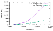
(a) Memory (dlp)

(b) Complexity (dlp)

(c) Memory (slp)

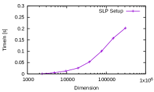
(d) Complexity (slp)

Figure 1: Memory and time per degree of freedom for the cube

To outline the results, Figure 1 shows the memory requirements per degree of freedom as function of $n$ for the single layer (c) and the double layer potential (a). In both cases from the beginning of our experiment the recompressed version needs less storage and the memory advantage improves with $n$.

The panels (b) and (d) in Figure 1 show the runtime per degree of freedom for the recompression of the $\mathcal{DH}^{2}$-matrix obtained by interpolation. Since we use a logarithmic scale for $n$ and a linear scale for the time divided by $n$, the experiment confirms our expectation of $\mathcal{O}(n\log n)$ complexity.

Even for higher wave numbers and other norms the algorithm keeps this behavior: Table LABEL:tab:slp_eucl shows results for doubled wave numbers on the unit sphere, where the error control strategy for the recompression uses the spectral norm instead of the Frobenius norm.

$$\begin{array}[]{r|r|r|r|r|r|r|r|r}&&\lx@intercol\hfil\text{original}\hfil\lx@intercol\vrule\lx@intercol&\lx@intercol\hfil\text{recomp.}\hfil\lx@intercol\vrule\lx@intercol&\\ n&\kappa&\text{basis}&\text{matrix}&\text{rank}&\text{basis}&\text{matrix}&\text{error}&\text{rel. error}\\ \hline\cr 2\,048&8&0.3&35.2&8&0.0&32.3&3.94_{-9\phantom{0}}&2.74_{-6}\\ \hline\cr 4\,608&12&1.3&82.9&9&0.1&71.3&3.22_{-9\phantom{0}}&6.65_{-6}\\ \hline\cr 8\,192&16&4.9&205.5&12&0.2&120.6&1.63_{-9\phantom{0}}&7.37_{-6}\\ \hline\cr 18\,432&24&10.1&821.9&15&0.6&223.0&1.26_{-9\phantom{0}}&1.66_{-5}\\ \hline\cr 32\,768&32&45.7&1\,450.8&15&1.7&312.3&6.15_{-10}&1.74_{-5}\\ \hline\cr 73\,728&48&72.7&3\,336.2&18&2.8&459.3&2.62_{-10}&2.16_{-5}\\ \hline\cr 131\,072&64&98.4&5\,114.2&21&3.9&586.7&1.49_{-10}&2.64_{-5}\\ \end{array}$$

Table 3: Single layer potential operator on the sphere (spectral norm)

Next we consider a more realistic geometry: a mesh of an airplane, more precisely a Boeing 747, comprised of $549\,836$ triangles and $274\,920$ vertices, provided by courtesy of Boris Dilba. We use the wave number $\kappa=3.15$, corresponding to a wavelength of approximately $2$. The maximal extent of the airplane is approximately $62$, i.e., approximately $31$ wavelengths. A picture of our object of study is shown in Figure 2.

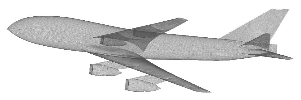
Figure 2: Mesh of a Boeing 747.

We have modified our recompression algorithm such that it can be applied during the set-up process to reduce intermediate storage requirements: the cluster basis is orthogonalized immediately, and the coupling matrices are constructed on the fly when needed during the recompression algorithm. With the modified algorithm we are able to set up the $\mathcal{DH}^{2}$-matrix with linear basis functions for the airplane mesh to obtain the results given in Table 4, where we have varied both the recompression tolerance $\epsilon$ and the interpolation order $m$. We also report run-times (in hours) measured on our shared-memory system.

$$\begin{array}[]{r|r|r|r|r|r|r|r}\epsilon&m&\text{time}&\text{rank}&\text{basis}&\text{matrix}&\text{error}&\text{rel. error}\\ \hline\cr 1.0_{-2}&4&0.5&28&1.7&83.6&1.0_{-3}&4.9_{-2}\\ \hline\cr 1.0_{-3}&5&1.3&38&2.9&105.9&1.8_{-4}&8.4_{-4}\\ \hline\cr 1.0_{-4}&6&3.2&46&4.7&138.4&3.1_{-5}&1.5_{-4}\\ \end{array}$$

Table 4: Boeing 747 with single layer potential (direct recompression)

We have measured the relative error between the dense, i.e., uncompressed, matrix and the recompressed approximation in the Frobenius norm. To put these results in perspective, the dense matrix takes about $4\,296$ KB per degree of freedom.

Compared to interpolation, our recompression algorithm reduces the storage requirements for the cluster basis from $194$ KB to $1.7$ KB for order $m=4$ and from $2\,137$ KB to $4.7$ KB for order $m=6$. For the coupling matrices, we save similar amounts of storage: we go from $2\,322$ KB to $83.6$ KB for order $m=4$ and from $25\,833$ KB to $138.4$ KB for order $m=6$. The measured relative Frobenius error is always well below the prescribed tolerance.

We can see that $\mathcal{DH}^{2}$-recompression is absolutely crucial in order to turn the initial approximation constructed by directional interpolation into a practically useful representation that saves approximately $96\%$ of storage at an accuracy of $3.1\times 10^{-5}$.

References

[1]
M. Bebendorf, C. Kuske, and R. Venn.
Wideband nested cross approximation for Helmholtz problems.
Num. Math., 130(1):1–34, 2015.
[2]
S. Börm.
Efficient Numerical Methods for Non-local Operators: -Matrix Compression, Algorithms and Analysis, volume 14 of EMS
Tracts in Mathematics.
EMS, 2010.
[3]
S. Börm.
Directional -matrix compression for high-frequency
problems.
Num. Lin. Alg. Appl., 24(6), 2017.
available online at http://dx.doi.org/10.1002/nla.2112.
[4]
S. Börm and J. M. Melenk.
Approximation of the high-frequency Helmholtz kernel by nested
directional interpolation: error analysis.
Num. Math., 137(1):1–34, 2017.
available at http://dx.doi.org/10.1007/s00211-017-0873-y.
[5]
A. Brandt.
Multilevel computations of integral transforms and particle
interactions with oscillatory kernels.
Comp. Phys. Comm., 65(1–3):24–38, 1991.
[6]
M. G. Duffy.
Quadrature over a pyramid or cube of integrands with a singularity at
a vertex.
SIAM J. Num. Anal., 19(6):1260–1262, 1982.
[7]
B. Engquist and L. Ying.
Fast directional multilevel algorithms for oscillatory kernels.
SIAM J. Sci. Comput., 29(4):1710–1737, 2007.
[8]
S. Erichsen and S. A. Sauter.
Efficient automatic quadrature in 3-d Galerkin BEM.
Comput. Meth. Appl. Mech. Eng., 157:215–224, 1998.
[9]
G. H. Golub and C. F. Van Loan.
Matrix Computations.
Johns Hopkins University Press, London, 1996.
[10]
L. Grasedyck and W. Hackbusch.
Construction and arithmetics of -matrices.
Computing, 70:295–334, 2003.
[11]
L. Greengard, J. Huang, V. Rokhlin, and S. Wandzura.
Accelerating fast multipole methods for the Helmholtz equation at
low frequencies.
IEEE Comp. Sci. Eng., 5(3):32–38, 1998.
[12]
L. Greengard and V. Rokhlin.
A fast algorithm for particle simulations.
J. Comp. Phys., 73:325–348, 1987.
[13]
W. Hackbusch.
A sparse matrix arithmetic based on -matrices. Part
I: Introduction to -matrices.
Computing, 62(2):89–108, 1999.
[14]
W. Hackbusch and B. N. Khoromskij.
A sparse matrix arithmetic based on -matrices. Part
II: Application to multi-dimensional problems.
Computing, 64:21–47, 2000.
[15]
W. Hackbusch and Z. P. Nowak.
On the fast matrix multiplication in the boundary element method by
panel clustering.
Numer. Math., 54(4):463–491, 1989.
[16]
M. Messner, M. Schanz, and E. Darve.
Fast directional multilevel summation for oscillatory kernels based
on Chebyshev interpolation.
J. Comp. Phys., 231(4):1175–1196, 2012.
[17]
E. Michielssen and A. Boag.
A multilevel matrix decomposition algorithm for analyzing scattering
from large structures.
IEEE Trans. Antennas and Propagation, AP-44:1086–1093, 1996.
[18]
V. Rokhlin.
Rapid solution of integral equations of classical potential theory.
J. Comp. Phys., 60:187–207, 1985.
[19]
V. Rokhlin.
Diagonal forms of translation operators for the Helmholtz equation
in three dimensions.
Appl. Comp. Harm. Anal., 1:82–93, 1993.
[20]
S. A. Sauter.
Variable order panel clustering.
Computing, 64:223–261, 2000.
[21]
S. A. Sauter and C. Schwab.
Boundary Element Methods.
Springer, 2011.