The PAU Survey: Early demonstration of photometric redshift performance in the COSMOS field

Abstract

The PAU Survey (PAUS) is an innovative photometric survey with 40 narrow bands at the William Herschel Telescope (WHT). The narrow bands are spaced at 100Å intervals covering the range 4500Å to 8500Å and, in combination with standard broad bands, enable excellent redshift precision. This paper describes the technique, galaxy templates and additional photometric calibration used to determine early photometric redshifts from PAUS. Using bcnz2, a new photometric redshift code developed for this purpose, we characterise the photometric redshift performance using PAUS data on the COSMOS field. Comparison to secure spectra from zCOSMOS DR3 shows that PAUS achieves $\sigma_{68}/(1+z)=0.0037$ to $i_{\mathrm{AB}}<22.5$ for the redshift range $0<z<1.2$, when selecting the best 50% of the sources based on a photometric redshift quality cut. Furthermore, a higher photo-z precision ($\sigma_{68}/(1+z)\sim 0.001$) is obtained for a bright and high quality selection, which is driven by the identification of emission lines. We conclude that PAUS meets its design goals, opening up a hitherto uncharted regime of deep, wide, and dense galaxy survey with precise redshifts that will provide unique insights into the formation, evolution and clustering of galaxies, as well as their intrinsic alignments.

1 Introduction

Wide-field galaxy surveys are critically important when studying the late-time universe. By mapping the positions, redshifts and shapes of galaxies, we are able to measure the statistical properties of the cosmological large-scale structure, which in turn allows us to make inferences on, for instance, the nature of dark energy and dark matter (Weinberg et al., 2013). In cosmology, these wide-field surveys are typically divided into two types: spectroscopic surveys and imaging surveys.

Deep spectroscopic redshift surveys typically cover relatively small areas, but with a high galaxy density (e.g. Davis et al., 2003; Lilly et al., 2007). Such observations have shown how the physical properties of galaxies depend on their environment and how these evolve over time (e.g. Tanaka et al., 2004). Such targeted studies, however, are limited to relatively small physical scales. In contrast, surveys probing large scales only sparsely sample the density field (e.g. Strauss et al., 2002). This allows them to infer cosmological parameters by mapping the spatial distribution of galaxies on large scales. Moreover, the targets are typically preselected, to efficiently get redshifts with minimum observation time (e.g. Jouvel et al., 2014).

Complete spectroscopic redshift coverage of a large area is difficult with current instrumentation. Multi-object fibre spectrographs on 4m class telescopes have surveyed large areas of sky, but fibre collisions limit the efficiency with which small scales can be probed. It is, however, possible to achieve a high spatial completeness as demonstrated by the Galaxy Mass Assembly (GAMA) survey (Driver et al., 2009). This project used the AAOmega spectrograph on the Anglo-Australian Telescope (AAT) to obtain $\sim 300,000$ spectroscopic redshifts down to $r<19.8$ mag over an area of almost 300 deg². Repeated observations allowed a 98% completeness down to the limiting magnitude. The bright limiting magnitude, however, limits the analysis to relatively low redshifts and relatively luminous galaxies. Large telescopes are needed to probe higher redshifts, but their field-of-view is typically too small to cover large areas.

As a consequence, the role of environment on intermediate to small scales (below 10-20 Mpc), i.e. the weakly non-linear regime, is not well studied. Interestingly this is where the statistical signal-to-noise is highest for large galaxy imaging surveys. To robustly separate cosmological and galaxy formation effects, we need to dramatically improve our understanding of these scales, where baryonic and environmental effects become relevant. This requires surveying large contiguous areas while simultaneously achieving a high density of galaxies with sub-percent photometric redshift accuracy. In this paper we present the first results of an alternative approach that enables us to survey large areas efficiently, whilst achieving excellent redshift precision for galaxies as faint as $i_{\mathrm{AB}}\sim 22.5$.

The Physics of the Accelerating Universe Survey (PAUS) at the William Herschel Telescope (WHT) uses the PAU Camera (PAUCam, Padilla et al., in prep.) to image the sky with 40 narrow bands (NB) that cover the wavelength range from 4500Å to 8500Å at 100Å intervals. These images are combined with existing deep broad band (BB) photometry. Based on simulations (Martí et al., 2014b), the expected photo-z precision is $\sigma_{68}/(1+z)=0.0035$ for $i<22.5$ for a 50% quality cut. The quality cut is based on the posterior distribution and does not use spectroscopic information. This precision corresponds to $\simeq 12$ Mpc/$h$ in comoving radial distance at $z=0.5$. The initial motivation to reach such precision was to be able to resolve the baryon acoustic oscillations (BAO) peak (Benítez et al., 2009; Gaztañaga, Cabré & Hui, 2009), but it also allows us to probe the start of the weakly non-linear regime for structure formation. Moreover, this precision is (nearly) optimal for many cosmological applications (Gaztañaga et al., 2012; Eriksen & Gaztañaga, 2015).

Cosmological redshifts are traditionally determined either from spectra or broad band photometry. The redshift precision that can be achieved using broad band photometry is typically $\sigma_{68}/(1+z)\simeq 0.05$ (e.g. Hildebrandt et al., 2012; Hoyle et al., 2018), while including infrared, ultra violet (UV) and intermediate bands can reduce the uncertainties by factors of a few (Laigle et al., 2016; Molino et al., 2014). The much higher wavelength resolution of spectrographs allows for a much improved determination of the locations of spectral features, resulting in high precision redshifts $\sigma_{68}/(1+z)\lesssim 0.001$. Many applications, however, do not require such precision and the predicted PAUS performance is more than adequate.

For instance, errors in photo-z estimates translate into errors in the luminosity or star formation rate (SFR). At $z=0.5$ the typical broad band photo-z uncertainty of $\sigma_{68}/(1+z)\simeq 0.05$ translates into a 40% error in the luminosity (or 355 Mpc/$h$ in luminosity distance), while the PAUS photo-z error corresponds to 2.5%, comparable to other sources of errors (such as flux calibration). For clustering measurements the improvement is even more important as the uncertainty in comoving radial distance is reduced by more than an order of magnitude from 171 Mpc to 12 Mpc, sufficient to trace the large-scale structure. The improvement provided by spectroscopic redshifts, which are typically ten times better, is therefore of limited use.

Even though PAUS will cover a modest area compared to large wide imaging surveys, PAUS will increase the number density of galaxies with sub-percent precision redshifts by nearly two orders of magnitude to tens of thousands of redshifts per square degree. Such redshift precision over a large area will allow a range of interesting studies. It enables the study of the clustering of galaxies in the transition from the linear to non-linear regime with high density sampling for several galaxy populations. This will also allow multiple tracer techniques over the same dark matter field (Eriksen & Gaztañaga, 2015; Alarcon, Eriksen & Gaztanaga, 2018).

An important application is the study of the intrinsic alignments of galaxies. These are an important tracer of the interactions between the cosmic large-scale structure and galaxy evolution processes (e.g. Catelan, Kamionkowski & Blandford, 2001; Heavens, Refregier & Heymans, 2000; Croft & Metzler, 2000; Hirata & Seljak, 2004; Joachimi et al., 2015; Troxel & Ishak, 2015). They are also a limiting astrophysical systematic in cosmic weak lensing surveys, especially for the next generation of dark energy missions, such as LSST (LSST Science Collaboration, 2009), Euclid (Laureijs et al., 2011) and WFIRST (Spergel et al., 2015). The depth of the PAUS data will push the measurements out to $z\sim 0.75$, allowing us to study the luminosity and redshift dependence of the signal, whilst at the same time probing a wide range of environments. By targeting fields for which high-quality shape measurements already exist (CFHTLS W1, W2, W3 and W4), PAUS is expected to achieve competitive intrinsic alignment measurements.

In this paper we present the first results for PAUS, demonstrating that we can indeed achieve the predicted redshift precision. The analysis in this paper is limited to PAUS observations of the COSMOS field. This is a well-studied area on the sky with a wide range of ancillary data, such as high-resolution HST imaging, and deep broad- and medium-band imaging data extending both towards UV and near infrared (NIR) wavelengths. Importantly for this study, extensive spectroscopy is available. This enables us to quantify the precision with which we can determine redshifts and compare the results to the predictions based on simulated data.

The structure of the paper is as follows. In §2 we give an overview of the PAUS data reduction and external data used. In §3 we present the PAUS data in the COSMOS fields and the PAUCam filters. We introduce the bcnz2 code in §4 and give additional details in Appendix A. Sections §5 and §6 details the photo-z results. Additional background material and results can be found in Appendices B and C.

2 Data

In §2.1 we briefly discuss the PAUS data reduction, while §2.2 presents the external broad band data. The spectroscopic redshift catalogue to validate the photo-z performance is described in §2.3.

2.1 Data reduction overview

To efficiently process the large amount of data from PAUS, a dedicated data management, reduction, and analysis pipeline has been developed (PAUdm). We refer the interested reader to the specific papers that describe the various steps in more detail, including the associated quality control.

Following the observations, the raw data are transferred and stored at Port d’Informació Científica (PIC) (Tonello et al., in prep.). The day after the data are taken, the images are processed there, using the nightly pipeline (Serrano et al., in prep.; Castander et al., in prep.). This pipeline performs basic instrumental de-trending processing, some specific scattered light correction and finally an astrometric and photometric calibration of the narrow band images.

The master bias is constructed from exposures, with a closed shutter and zero exposure time, using the median of at least five images. Images are then flattened using dome flats, obtained by imaging a uniformly illuminated screen. Cosmic rays are removed with Laplacian edge detection (van Dokkum, 2001). A final mask also removes the saturated pixels.

In order to properly align the multiple exposures an astrometric solution is added. We use the astromatic software (sextractor, scamp, psfex Bertin, 2011). An initial catalogue is created using sextractor (Bertin & Arnouts, 1996). The astrometric solution is then found using scamp by comparing to Gaia DR1(Gaia Collaboration, 2016). Furthermore, the point spread function (PSF) is modelled with psfex. Stars in the COSMOS field are identified through point-sources in the COSMOS-Advanced Camera for Surveys (ACS) (Koekemoer et al., 2007; Leauthaud et al., 2007), as available from Laigle et al. (2016) (hereafter COSMOS2015). For the wide fields, we have developed a new method, separating stars and galaxies with convolutional neural networks (CNN) using the the narrow band data (Cabayol et al., 2018).

PAUS is calibrated relative to the Sloan Digital Sky Survey (SDSS) (Castander et al., in prep.). Stars in the overlapping area with $i<21$ are fitted with the Pickles stellar templates (Pickles, 1998) using the SDSS u,g,r,i and z bands (Smith et al., 2002). The corresponding spectral energy distribution (SED) and best fit amplitude then provide a model flux in the narrow bands. To ensure a robust solution, we limit the calibration to stars with $\mathrm{SNR}>10$ in the narrow band and $i_{\mathrm{AB}}<21$. A single zero-point per image is determined by comparing the model and observed fluxes. The calibration step removes the Milky Way (MW) extinction. When fitting to SDSS, the model includes extinction. For the correction we use the corresponding model without extinction.

The galaxy fluxes are measured by the memba pipeline (Serrano et al., in prep.). Deeper broad band (BB) data exist for both COSMOS and the wide fields. Hence the galaxy positions are determined a priori using these data and the narrow-band (NB) fluxes are determined using forced photometry by placing a suitable aperture on the NB images, centred on these positions. To provide consistent colours, we match the aperture to the size of the galaxy of interest, using the r50 deconvolved measurement from COSMOS ACS. In the case of the COSMOS data the size and elliptical shape used comes from the COSMOS Zurich catalogue (Sargent et al., 2007). The elliptical aperture in memba is scaled using both the size and PSF FWHM to target 62.5% of the total flux. While the optimal SNR depends on the galaxy light profile and Sersic index, this fraction is close to optimal.

Fluxes are measured on individual exposures, where the background is determined using an annulus from 30 to 45 pixels around the galaxies. The galaxies falling into the background annulus are removed with a sigma-clipping. The fluxes are thus background subtracted, scaled with the image zero-points and then combined with a weighted mean into coadded fluxes.

2.2 External broad bands

We used the BB data from the COSMOS2015 catalogue. It includes $u^{*}$ band data from the Canada-France Hawaii Telescope (CHFT/MegaCam) and B, V, r, $i^{+}$, $z^{++}$ broad band data from Subaru, obtained as part of the COSMOS-20 survey (Taniguchi et al., 2015). Figure 14 shows the broad band transmission curves. We use the 3” diameter PSF homogenised flux measurements available in the catalogue release and apply several corrections as described and provided in COSMOS2015.

The Milky Way interstellar dust reddens the observed spectrum of background galaxies. As described in the previous subsection, PAUS data are corrected for dust extinction in the calibration. Therefore we need to do the same for COSMOS data. Each galaxy has an $E(B-V)$ value from a dust map (Schlegel, Finkbeiner & Davis, 1998), and Laigle et al. (2016) provide an effective factor $F_{x}$ for each filter $x$ according to Allen (1976). For each galaxy the corrected magnitudes are

$$\text{Mag corrected}_{x}=\text{Mag uncorrected}_{x}-E(B-V)*F_{x}.$$ (1)

Photometric offsets are added to acquire total fluxes as described in Laigle et al. (2016). This is not strictly needed since the photometric code estimates a zero-point shift between the broad and narrow band systems per galaxy (see §4.2).

2.3 Spectroscopic catalogue

To determine the accuracy of the photometric redshift estimation using PAUS, we compare to zCOSMOS DR3 bright spectroscopic data, which has a pure magnitude selection in the range $15<i_{\mathrm{AB}}<22.5$ (Lilly et al., 2007). This selection yields a sample mainly covering the redshift range $0.1\lesssim z\lesssim 1.2$ in 1.7 deg² of the COSMOS field ($149.47\degree\lesssim\alpha\lesssim 150.77\degree$, $1.62\degree\lesssim\delta\lesssim 2.83\degree$ Knobel et al., 2012).

This dataset contains 16885 objects of which 10801 remain after removing less reliable redshifts based on a provided confidence class ($3\leq\mathrm{CLASS}<5$ Lilly et al., 2009). This sample covers most of the redshift and magnitude range for PAUS, which makes it especially interesting for validating the photometric redshift precision. The spectroscopic completeness is shown in Figure 13.

3 PAUCam data in the COSMOS field

As the start of the survey suffered from adverse weather conditions, the data for the COSMOS field were collected over a longer period in the semesters 2015B, 2016A, 2016B and 2017B. As detailed in Madrid et al. (2010); Castander & et al. (2012); Padilla et al. (in prep.), the narrow-band filters are distributed through 5 interchangeable trays, each carrying a group of 8 NB filters consecutive in wavelength. Each position is imaged with exposure times of 70, 80, 90, 110 and 130 seconds, from the bluest to the reddest tray. The COSMOS field was divided into 390 pointings, each observed with between 3 and 5 dithers for each of the 5 narrow-band filter trays. The final data set, which lacks some pointings, comprises a total of 9715 exposures.

3.1 Filter transmission curves

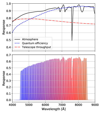
Figure 1: Top: The atmosphere, quantum efficiency and telescope throughput. Bottom: The throughput of the PAUS narrow bands when combining the filter transmission and the effects in the top panel.

The PAUCam (Padilla et al., in prep.) instrument at the William Herschel Telescope (WHT) has a novel set of 40 narrow band and 6 broad band filters. The total narrow band transmission includes filters, atmosphere, instrument and telescope effects. Figure 1 shows the filter transmission curves, where the top panel shows the effect of the atmospheric transmission. As a preliminary solution we used the Apache Point Observatory (APO) transmission and will update this in due course. Any residual differences are removed in the calibration step comparing with reference standard stars (see Castander et al., in prep.). The quantum efficiency (blue line) of the Hamamatsu CCDs has been measured at the IFAE laboratories (Casas et al., 2014), while for the telescope throughput (red line) we use the publicly available transmission for the WHT.

In the bottom panel of Figure 1, the narrow band throughput is shown, including the effects mentioned above combined with filter transmission. The optical filters, are 130Å (FWHM) wide and equally spaced (100Å) in the range between 4500Å and 8500Å. The transmission was measured in the CIEMAT optical laboratory and shifted to the PAUCam operating temperatures using a theoretical relation (Casas et al., 2016).

3.2 Signal to noise ratio

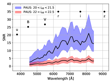
Figure 2: The SNR per exposure distribution on the COSMOS field. Two lines shows the median SNR in a bright and faint subsample. The surrounding shaded band shows the area between 16 and 84 percentiles. For the broad bands, we only show the median SNR of the faintest subsample.

The typical SNR (flux/error) per exposure of the narrow band flux measurements is low, in particular at bluer wavelengths. The redder NBs are sky limited, while the bluer bands are limited by the readout noise. For the wide fields the exposure times were adapted to adjust for this lack of SNR in the bluer bands. This is evident from Figure 2, which shows the SNR for the PAUCam data we use here. To illustrate the trends, the data are split into a bright ($20<i_{\mathrm{AB}}<21.5$) and faint ($22<i_{\mathrm{AB}}<22.5$) subsample. The lines indicate the median SNR, while the filled bands show the corresponding 16 and 84 percentiles.

In the bright subsample ($20<i_{\mathrm{AB}}<21.5$), the median SNR increases from 2.7 to 14.5 from the bluest (NB455) to the reddest (NB855) band. Each tray contains 8 filters, so it is not possible to optimise the exposure time for each filter. Moreover, most of the galaxies have red SEDs and thus are brighter in the reddest bands.

The faint subsample ($22<i_{\mathrm{AB}}<22.5$) has a much lower SNR. As a result, flux estimates can become negative due to noise. The median SNR in this plot ranges from 0.9 to 3.3, from the bluest to the reddest band. It is important that the photo-z codes properly handle the low SNR for individual NB measurements, as they still contain information.

The black points in Figure 2 indicate the median SNR measured in the COSMOS2015 BB data for the faint sample. We limit the precision of these measurement to 3% for all bands (see §4), i.e. limiting the SNR to 35. This ensures that the broad band data do not dominate the fits as the uncertainties for some of the BB data appear to be underestimated (Laigle et al., 2016). The SNR of the BB data is about 8 times higher than with the narrow bands, which can pose challenges for the photo-z determination. For instance, it requires a careful calibration between the bands (§4.2).

4 Photometric redshift estimation

Photometric redshift can be determined using a variety of approaches, and consequently different public photo-z codes are available. Examples of template-based codes include bpz (Benítez, 2000) and lephare (Arnouts & Ilbert, 2011). These compare the observations to predefined redshift dependent models. Using machine learning the skynet (Bonnett, 2015), annz2 (Sadeh, Abdalla & Lahav, 2016), and dnf (De Vicente, Sánchez & Sevilla-Noarbe, 2016) codes can learn the relation between flux and redshift.

While the public bpz code was used in Martí et al. (2014b), it does not include emission lines in a flexible way (§4.5). These lines are critical for achieving the required precision. This paper introduce bcnz2, a new code specifically developed for the challenges found using PAUS data.

4.1 Model flux estimation

The bcnz2 is a template based photometric redshift code, that compares the observed flux in multiple bands with redshift dependent models of the galaxy flux. The observed flux is a wavelength dependent convolution of the galaxy SED and the response of the detector. Let $f_{\lambda}(\lambda)$ be the galaxy SED, which is the flux a galaxy transmits at a wavelength $\lambda$. With the expansion of the Universe, a photon emitted at $\lambda_{e}$ is observed at $\lambda_{o}=(1+z)\lambda_{e}$. The observed photon flux ($f_{i}$) in a fixed band is (Hogg et al., 2002; Martí et al., 2014b)

$$f_{i}=\int_{0}^{\infty}\mathrm{d}\lambda\,\lambda f_{\lambda}(\lambda)R_{i}(\lambda),$$ (2)

where $R_{i}(\lambda)$ is the system response which is a multiplicative combination of atmospheric, telescope, CCD detector and filter transmission (§3.1). The galaxy SEDs $f_{\lambda}(\lambda)$ used are described in §4.4.

4.2 Photo-z formalism

The bcnz2 photo-z algorithm uses a linear combination of templates in order to fit the measured fluxes. For each galaxy, we estimate the redshift probability distribution $p(z)$ for a given galaxy defined as:

$$p(z)\propto\underset{{\bm{\alpha}}_{1}\geq 0}{\int\mathrm{d}{\bm{\alpha}}_{1}}\dots\underset{{\bm{\alpha}}_{n}\geq 0}{\int\mathrm{d}{\bm{\alpha}}_{n}}\exp\left(-0.5\chi^{2}[z,{\bm{\alpha}}]\right)p_{\mathrm{Prior}}(z,{\bm{\alpha}}),$$ (3)

where $p_{\mathrm{Prior}}(z,{\bm{\alpha}})$ are the general form of the priors and $n$ is the number of templates. Here, as described in §4.3.1, the integration is restricted to positive normalisation of the templates (${\bm{\alpha}}_{i}$). Further, we define

$$\chi^{2}[z,{\bm{\alpha}}]=\sum_{i,NB}\left(\frac{\tilde{f_{i}}-l_{i}kf^{\mathrm{Model}}_{i}}{\sigma_{i}}\right)^{2}+\sum_{i,BB}\left(\frac{\tilde{f_{i}}-l_{i}f^{\mathrm{Model}}_{i}}{\sigma_{i}}\right)^{2},$$ (4)

where $l_{i}$ and $k$ are calibration factors, which are explained later. Here $\tilde{f}_{i}$ is the observed flux in band $i$, $\sigma_{i}$ is the corresponding error. The model flux, $f^{\mathrm{Model}}_{i}$, is defined by

$$f^{\mathrm{Model}}_{i}[z,{\bm{\alpha}}]\equiv\sum_{j=1}^{n}f^{j}_{i}(z){\bm{\alpha}}_{j},$$ (5)

where $f_{i}^{j}$ is the model flux of template $j$ in band $i$, with amplitude ${\bm{\alpha}}_{j}$. The final template is therefore a linear combination of templates, which are defined in §4.4. This approach is similar to that of eazy (Brammer, van Dokkum & Coppi, 2008).

COSMOS photometry uses fixed apertures rescaled to total flux, while PAUS uses matched apertures (see §2.1). Furthermore, an uncertainty in the flux fraction introduces an uncertainty when scaling to total flux. To match the narrow and broad band systems, we consider the scaling $k$ (§4.3.3) as a free parameter per galaxy.

In addition, Eq. (4) contains a global zero-point $l_{i}$ for each band $i$. The PAU survey relies on external observations for the broad bands. This might mean different photometry, including different aperture sizes. As described §4.3.4, we therefore want to determine a zero-point correction ($l_{i}$) for each band. This will be the same for all galaxies.

4.3 Photo-z algorithm

4.3.1 P(z) approximation

Integrating over all amplitudes in Eq. (3) is numerically expensive and makes us sensitive to the priors. While a closed-form solution exists, this allows for negative amplitudes (${\bm{\alpha}}$). In practice allowing for negative amplitudes introduces too much freedom, which degrades the redshift precision. Allowing for negative amplitudes would e.g. lead to the OIII line template fitting to spurious low flux measurements caused by negative (inter-CCD) cross-talk. Some of the positive amplitude combinations should also be prevented, e.g. through a more physical modelling of the SEDs, in future work. We therefore approximate:

$$p(z) \propto\underset{{\bm{\alpha}}_{1}\geq 0}{\int\mathrm{d}{\bm{\alpha}}_{1}}\dots\underset{{\bm{\alpha}}_{n}\geq 0}{\int\mathrm{d}{\bm{\alpha}}_{n}}\exp\left(-0.5\chi^{2}[z,{\bm{\alpha}}]\right)p_{\mathrm{Prior}}(z,{\bm{\alpha}})$$ (6)

$$\approx\exp(-0.5\chi^{2}_{\mathrm{Min}}[z]),$$ (7)

where the integral at each redshift is approximated using the maximum likelihood conditional on $z$ (min $\chi^{2}$), with the proportionality constant being determined by requiring that $p(z)$ integrates to unity. While this approximation only uses the peak position, we find that this works sufficiently well.

4.3.2 P(z) estimation (per galaxy)

The minimum is determined using the algorithm of Sha et al. (2007). This algorithm ensures the amplitudes ${\bm{\alpha}}$ remain positive. It is also proven to converge towards the global minimum of $\chi^{2}[z,{\bm{\alpha}}]$ for a fixed redshift $z$. We therefore minimise the $\chi^{2}$ expression with respect to the amplitudes (${\bm{\alpha}}$) on a redshift grid in the redshift range $0.01<z<1.2$, using $\Delta z=0.001$ wide redshift bins. For further details see Appendix B.

4.3.3 COSMOS/PAU calibration (per galaxy)

The minimisation algorithm relies on the $\chi^{2}$ expression being on a quadratic form. Extending to also determining $k$ (Eq. 3), the galaxywise scaling between the narrow and broad band photometry is therefore not straightforward. Instead, using the derivative of the $\chi^{2}$ relation (Eq. 3) with respect to $k$, one can find the solution which minimises the $\chi^{2}$ value. This gives the solution

$$k=\frac{\sum_{i,\mathrm{NB}}\tilde{f}_{i}l_{i}f^{\mathrm{Model}}_{i}/\sigma_{i}^{2}}{\sum_{i,\mathrm{NB}}{(l_{i}f^{\mathrm{Model}}_{i})}^{2}/\sigma_{i}^{2}},$$ (8)

where the sum over filters only includes the narrow bands. Also, to lower the runtime, we only estimate the zero-point $k$ at every tenth step in the iterative minimisation (of ${\bm{\alpha}}$), as described in §4.3.2.

4.3.4 Zero point recalibration (per band)

To determine the zero-points per band ($l$), a common approach is to compare the photo-z code best fit model with the observed fluxes (Benítez, 2000). This ratio can be used to determine a zero-point offset per band. To estimate the bandwise zero-points, we only estimate the best fit model at the spectroscopic redshift. This reduces the runtime by three orders of magnitude, since one only has to evaluate the fit at one redshift per galaxy. After determining the best fit model ($f^{\mathrm{Model}}$) by running the photo-z code for a fixed spectroscopic redshift, one finds the zero-point in band $i$ by

$$l_{i}=\mathrm{Median}[f^{\mathrm{Model}}/f^{\mathrm{Obs}}],$$ (9)

where we use the median, instead of a weighted mean, because it reduces the impact of outliers. When using spectroscopic redshifts, one should in theory split into a training and validation sample. However, unlike e.g. machine learning redshifts, we train one number per band and not per galaxy. The zero-points are therefore less affected by overfitting. We have tested that this does not significantly affect the results and we therefore do not split the catalogue by default.

The photo-z code is first run 20 times at the spectroscopic redshift. At the start the offsets per band, $l_{i}$, are assumed unity and they are updated after each iteration using Eq. (9). In this process the scaling $k$ is kept free. Afterwards we run the photo-z using the final zero-points ($l_{i}$), also treating $k$ as a free parameter.

4.4 Combination of SEDs

The basic formalism of using a linear combination of templates has a problem when including intrinsic extinction (Appendix C). The dust extinction is not an additional template, but a wavelength dependent effect that multiplicatively changes the SEDs. The simplest solution is to generate new SEDs for different extinction laws and extinction values ($E(B-V)$). These can then directly be used in the photo-z code. While possible in theory, we find that this gives too much freedom, reducing the photo-z performance.

Instead, we add priors to restrict the possible SED combinations. The minimisation algorithm limits our choice of priors. We group together the SEDs in different sets, discussed later in this subsection. Within these sets the prior is unity, but zero outside. This can be used both to avoid combining different $E(B-V)$ values and unphysical template combinations. Using this prior, Eq. (3) reduces to

$$p(z) \propto\sum_{\mu}\int\mathrm{d}{\bm{\alpha}}^{\mu}_{1}\dots\int\mathrm{d}{\bm{\alpha}}^{\mu}_{n}\exp(-0.5\chi^{2}[z,{\bm{\alpha}}^{\mu}])$$ (10)

$$\approx\sum_{\mu}\exp\left(-0.5\chi^{2}_{\mathrm{Min\,{\bm{\alpha}}^{\mu}}}[z]\right),$$ (11)

where the sum is over different sets of SEDs (${\bm{\alpha}}^{\mu}$) (which we call runs), with the approximation being the same as in Eq. (7). In practice, this means one can separately run the photo-z code for many different SED combinations and then combine them later (Eq. 11).

Run #	Lines	Ext law	SED
1	False	None	Ell1, Ell2, Ell3, Ell4, Ell5, Ell6
2	False	None	Ell6, Ell7, S0, Sa, Sb, Sc
3	True	None	Sc, Sd, Sdm, SB0, SB1, SB2
4	True	None	SB2, SB3, SB4, SB5, SB6, SB7, SB8, SB9, SB10, SB11
5	False	None	BC03(0.008, 0.509), BC03(0.008, 8.0), BC03(0.02, 0.509), BC03(0.02, 2.1), BC03(0.02, 2.6), BC03(0.02, 3.75)
6-15	True	Calzetti	SB4, SB5, SB6, SB7, SB8, SB9, SB10, SB11
16-25	True	Calzetti+Bump 1	SB4, SB5, SB6, SB7, SB8, SB9, SB10, SB11
26-35	True	Calzetti+Bump 2	SB4, SB5, SB6, SB7, SB8, SB9, SB10, SB11

Table 1: The configurations used for the photo-z code. In the first column is the configuration number, while the second gives whether emission line templates are added. A third column gives the extinction law, which is used for $E(B-V)$ values between 0.05 and 0.5, with 0.05 spacing. The SB templates are from the BC03 library. In run #5 we use six additional BC03 templates, with their metallicity (Z) and age (Gyr) specified in parenthesis. When running with the Calzetti law (#6-35), we also include two variations with a 2175Å bump (see Appendix C).

Table 1 describes the SED and extinction combinations that are used when running the photo-z code. For the case of elliptical and red spiral galaxy templates (run #1-2), we neither include emission lines nor dust extinction. For starburst galaxies, as used in run #3-4, Ilbert et al. (2009) had problems reproducing the bluest colours in the spectroscopic sample. Following that paper, we use 12 starburst galaxies generated by the Bruzual & Charlot (2003) models. These have ages spanning from 3 Gyr to 0.03 Gyr. Combining run #1-2 and #3-4 slightly decreases the photo-z performance.

Following Ilbert et al. (2013) and Laigle et al. (2016), we include a new set of BC03 templates (run #5) assuming an exponentially declining SFR with a short timescale $\tau=0.3$ Gyr to account for a missing population of quiescent galaxies. In addition, starburst templates are run using the Calzetti extinction law (Calzetti et al., 2000) and the two modified versions (Appendix C) with $E(B-V)$ values between 0.05 and $0.5$ in 10 steps (run #6-35).

4.5 Emission lines

	$\lambda[\mathrm{\AA}]$	Template 1	Template 2
${\mathrm{H}}_{\alpha}$	6563	1.77	-
${\mathrm{H}}_{\beta}$	4861	0.61	-
${\mathrm{Ly}}_{\alpha}$	1216	2	-
${\mathrm{NII}}_{1}$	6548	0.19	-
${\mathrm{NII}}_{2}$	6583	0.62	-
OII	3727	1	-
${\mathrm{OIII}}_{1}$	4959	-	1
${\mathrm{OIII}}_{2}$	5007	-	3
${\mathrm{SII}}_{1}$	6716	0.35	-
${\mathrm{SII}}_{2}$	6731	0.35	-

Table 2: Emission line ratios. In the second column is the central wavelength. The third column contains the main emission line template, with flux ratios relative to $\mathrm{OII}$. In the last column is the OIII template, normalized relative to ${\mathrm{OIII}}_{1}$.

Table 2 contains the set of emission lines that are used in this paper. The emission lines are parameterised using a set of fixed amplitude flux-ratios. These are obtained from COSMOS2015 (Laigle et al., 2016) and references therein. When estimating the fluxes, we approximate the emission lines as a delta function. In this table, the fluxes are normalised to the OII values. Beck et al. (2016) found comparable ratios.

The inclusion of emission lines can be done in different ways. One approach is to add the emission lines as an additional separate SED. This can be thought of as having a contribution from a very young stellar population. We have added the emission lines using two templates, one that contains all emission lines in Table 2, except the OIII doublet, which is kept in a separate template. This is needed to take into account the large variability between OIII and $\text{H}_{\beta}$ lines. Running with a single emission line template led to a significant degradation in the photo-z performance. So far we have used common practice and not included BPT (Baldwin, Phillips & Terlevich, 1981) information. Better modelling of emission lines is expected in future developments.

5 Results

In this section we present the main photo-z results (§5.1) and the additional calibration (§5.2). The benefits of combining broad and narrow bands are discussed (§5.3), before describing priors (§5.4) and quality cuts (§5.5). We validate the Probability Density Function (pdf) in §5.6.

5.1 Photo-z scatter and outliers

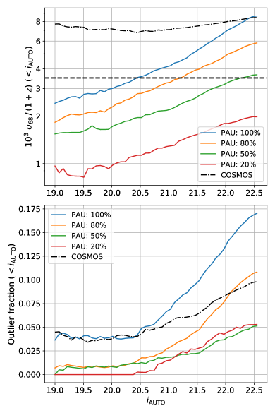
Figure 3: The $\sigma_{68}/(1+z)$ (top) and outlier fraction (bottom) for different quality cuts as a function of the cumulative magnitude bins. The solid lines show the results when 100, 80, 50 and 20 percent of the sample remain after a quality cut. The dashed line shows the COSMOS results without any quality cuts, using the public COSMOS2015 catalogue.

Figure 3 shows the main result of this paper: $\sigma_{68}$ and outlier fraction for PAUS and the COSMOS data. To quantify the photo-z precision, we use

$$\sigma_{68}\equiv 0.5\left(z^{84.1}_{\mathrm{quant}}-z^{15.9}_{\mathrm{quant}}\right)$$ (12)

which equals the dispersion for a Gaussian distribution, but is less affected by outliers. A galaxy is considered an outlier if

$$|z_{\mathrm{p}}-z_{\mathrm{s}}|\,/\,(1+z_{\mathrm{s}})>0.02,$$ (13)

where $z_{\mathrm{p}}$ and $z_{\mathrm{s}}$ are the photometric and spectroscopic redshifts, respectively.

The COSMOS result uses the redshift estimate (zp_gal) available in the COSMOS2015 catalogue. The PAUS results are given for different fractions that remain after a quality cut (Qz) (see §5.5) based on PAUS fluxes. Attempting to cut the COSMOS photo-z by the $p(z)$ quantiles ($z^{99}_{\mathrm{quant}}-z^{1}_{\mathrm{quant}}$) did not significantly change their photo-z precision. We therefore only show the COSMOS results for the full sample. The ALHAMBRA survey (Moles et al., 2008) result is not shown, since the public photo-z are worse than the COSMOS photo-z.

For $\sigma_{68}$ the horizontal lines marks the expected photo-z scatter of $\sigma_{68}/(1+z)=0.0035$ based on simulations at 50% cut (Martí et al., 2014b). The PAUS photo-z is close to reaching this value, achieving $\sigma_{68}/(1+z)\sim 0.0037$ for 50% of the galaxies with $i_{\mathrm{AB}}<22.5$ and the spectroscopic selection shown in Figure 13. Here the median $i_{\mathrm{AUTO}}$ is 20.6, 20.8, 21.2 and 21.4 for the 20, 50, 80 and 100 percent cuts, respectively. The corresponding figure in differential magnitude bins and photo-z scatter plot are included in Appendix B.

When applying a more stringent quality cut leaving less of the sample, the $\sigma_{68}$ is approaching $0.001(1+z)$ for a bright selection and increases to $0.002(1+z)$ for $i_{\mathrm{AB}}<22.5$. While the selection on the quality parameter results in selecting brighter galaxies, this population of galaxies with quasi-spectroscopic redshifts was never seen in simulations (Martí et al., 2014b). Even when running bpz on a noiseless catalogue, the $\sigma_{68}$ was never below $0.002(1+z)$. This mainly comes from emission lines not being properly included in the simulations.

The bottom panel of Figure 3 shows the corresponding outlier fraction. For the full sample, the PAUS photo-z has 18% outliers for $i_{\mathrm{AB}}<22.5$. This is higher than for COSMOS. Applying the quality cut lowers the outlier rate to a more reasonable level. One should keep in mind that the outlier rate is expected to reduce with better data reductions and improvements to the photo-z code.

5.2 Zero-points between systems

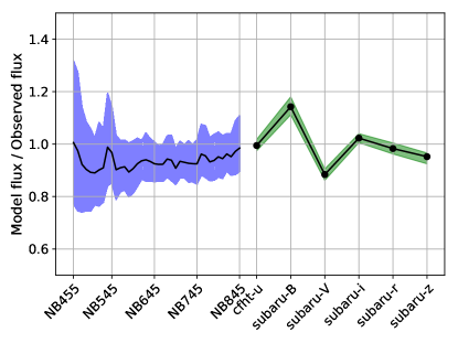
Figure 4: The bandwise calibrations for the narrow (hatched) and broad (solid) bands. On the x-axis is the band, while the y-axis shows the zero-points. The solid line shows the median zero-point, while the bands show the 16 to 86 percentile interval.

Figure 4 shows the recovered zero-points ($l_{i}$) from the photo-z code. PAUS is already calibrated relative to SDSS stars, which have a higher signal-to-noise ratio. One could restrict the additional zero-point calibration to determining the BB zero-point from a model fit to the NB. In practice we find better results from fitting to both NB and BB data, applying zero-points to both systems. Including the BB decreases the model fit uncertainty, but then includes bands which might require an offset. We handle this by repeatedly estimating the best fit model and applying the resulting offsets. By default this procedure is run with 20 iterations.

The x-axis shows the band, starting with the narrow band first and then the uBVriz bands. The coloured band shows the region between 16 and 84 percentiles of the offsets obtained from different galaxies in the last iteration step. Here and in the final zero-points, we have only included measurements with $\mathrm{SNR}>1$. While the spread for individual galaxies is quite large, the mean value of the sample is centred around unity. For the narrow bands there is a tilt at the blue end. When estimating the zero-points with only narrow bands (not shown), the BB zero-points only change slightly.

5.3 Combining broad and narrow bands

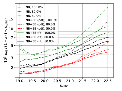
Figure 5: The impact on photo-z precision of different approaches to combine NB and BB information. The dotted lines show the narrow band performance alone, while dashed lines (pdf) combine the NB and BB pdfs. The solid lines (fit) simultaneously fit the narrow and broad bands.

While the narrow bands are important, the broad bands also contribute to photo-z precision. The broad bands have higher SNR (Fig. 2) and cover a larger wavelength range (Fig. 1). Qualitatively, these determine the best fit SED and a broad redshift distribution, which acts as a prior for the narrow bands. The narrow bands with good spectral resolution then determine the redshift more precisely. Without the broad bands, the photo-z code ended up confusing different emission lines. In particular, it confused OIII and $\mathrm{H_{\alpha}}$, which led to redshift outliers with $(z_{\mathrm{p}}-z_{\mathrm{s}})/(1+z_{\mathrm{s}})\approx\pm 0.15$, with more galaxies being scattered to lower redshift. Adding the broad bands effectively solves this problem.

Figure 5 compares different ways of including the broad band information in the photo-z code. The dotted lines show $\sigma_{68}/(1+z)$ when using narrow bands only. When running with NB alone, we combine the two emission line templates. Then the combination with broad bands is done in two different ways. First, we estimate the photo-z independently for the narrow and broad bands. These are then combined by multiplying the pdfs

$$p(z)=p_{\mathrm{NB}}(z)\times p_{\mathrm{BB}}(z),$$ (14)

which is only approximately correct, since we have marginalized over the SEDs independently for both runs. When adding the broad bands there is a significant improvement in photo-z performance for all selection fractions. The correct and more optimal approach is to estimate the photo-z, including both the broad and narrow bands. This jointly constrains both the redshift and SED combination from both systems, leading to a further decrease in the photo-z scatter. Fitting NB+BB is better than combining pdfs of separate NB and BB fits. In Figure 5 the 20% lines were removed, since they looked similar for all methods.

5.4 Photo-z priors

	No priors	SED priors	SED,z priors
Fraction
100%	8.5	8.5	8.3
80%	6.2	6.1	5.9
50%	3.9	3.9	3.7
20%	2.2	2.1	2.1

Table 3: The ${10}^{3}\ \sigma_{68}/(1+z)$ values for different priors. The first column gives the fraction of galaxies remaining after a quality cut (Qz), while the second is the result without priors. In the third column the priors are only applied to the SED combinations, while a fourth column adds priors (independently) on both the SED and redshift.

Template-based photometric redshift codes estimate the redshift by comparing the observations to model fluxes, estimated by redshifting templates. Estimating the redshift distribution requires, if using Bayesian methodology, the inclusion of priors. These can significantly improve the redshift estimation. When observing galaxies in a few colours or a restricted wavelength range, some low and high redshift models have similar colours. A prior based on luminosity functions effectively determines which solution is most probable (Benítez, 2000). In this paper we include priors on redshift and SEDs, but not on luminosity.

The PAU Survey observes galaxies with 40 narrow bands and combines these with traditional broad bands. In addition, the PAU Survey mostly observes galaxies in the redshift range $0<z<1.2$. Our redshift estimates should therefore be less sensitive to colour degeneracies. However, we attempt to further improve the redshifts by adding priors, constructed from the ensemble of galaxies.

The algorithm used when estimating the photometric redshift relies on the $\chi^{2}$ expression to be quadratic in the model amplitudes (see §4). This would make adding priors on the detailed SED combinations difficult. However, we can add priors on the different photo-z runs (Table 1). This effectively adds priors on the galaxy SED, the extinction law and the $E(B-V)$ value.

Table 3 compares the photo-z scatter for different priors (columns) and fractions remaining after a quality cut (first column). The priors for individual galaxies are constructed from the ensemble of galaxies. After running the photo-z code once, we construct the priors combining the probability for all galaxies. The second column gives $\sigma_{68}/(1+z)$ without priors, while the third column adds priors on each photo-z run. These are obtained by first running the photo-z without priors and then construct priors by the amount of galaxies having a minimum $\chi^{2}$ corresponding to each of the photo-z runs. This gives a minor improvement for 100 percent of the sample.

Similarly, the last column combines priors on SEDs and the redshift distribution. The optimal approach is to construct priors on both SEDs and redshifts combined, but this led to a too noisy distribution, for too few galaxies. Instead we combine the previous SED priors with a redshift prior as independent priors. The redshift priors are constructed from the redshift distribution obtained without a prior, convolved with a $\sigma_{\mathrm{z}}=0.003$ Gaussian filter to smooth the distribution. The final priors improve the photo-z for all selection fractions. This effectively also incorporates some clustering information from the field.

5.5 Quality cuts

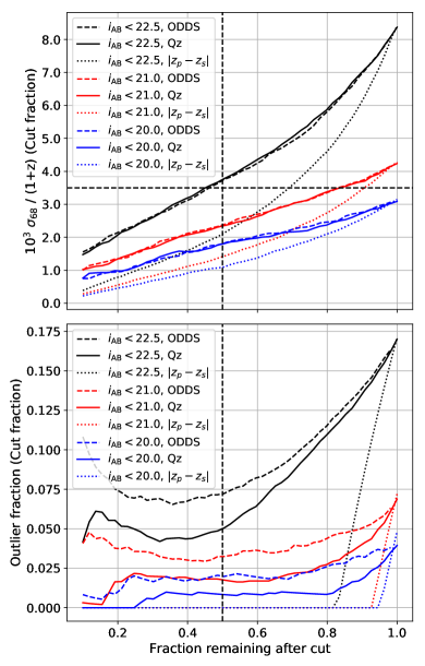
Figure 6: The $\sigma_{68}$ (top) and outlier fraction (bottom) for different magnitude limited samples and quality cuts as a function of the cut fraction. The results are shown for the three magnitude cuts: $i_{\mathrm{AB}}<20,21,22.5$ and two quality estimators: ODDS, Qz. Here $z_{p}-z_{s}$, which cuts on the absolute different between the photometric and spectroscopic redshift, is included as a reference. The horizontal dashed line (top panel) shows the nominal PAUS photo-z precision target for a 50% quality cut.

For different purposes, one might want to select a subsample with better photo-z precision (Elvin-Poole et al., 2018). A frequently used photo-z quality parameter is the ODDS parameter (Benítez, 2000) (bpz). The ODDS is defined as

$$\mathrm{ODDS}\equiv\int_{\mathrm{z_{b}-\Delta z}}^{\mathrm{z_{b}+\Delta z}}\mathrm{d}z\ p(z),$$ (15)

where $z_{b}$ is the posterior redshift mode (peak in $p(z)$) and $\mathrm{\Delta z}$ defines an interval around the peak, typically related to the photo-z scatter. This definition measures the fraction of the $p(z)$ located around the redshift peak, which e.g. can be used to remove galaxies with double peaked distributions. In this paper we use $\mathrm{\Delta z}=0.0035$, which is reduced from typical broad band values since the PAUS pdfs are narrower.

One should be aware that such a selection can introduce inhomogeneities. The photometric redshift quality flags depend on the data quality, the galaxy SED, the modelling and the photo-z method. A selection with a photo-z quality cut can indirectly cut on any or all of these quantities. As an example, Martí et al. (2014a) found that cutting on ODDS resulted in a spatial pattern corresponding to scanning stripes in SDSS data.

The ODDS quality parameter contains information on the redshift uncertainty, as described by the posterior $p(z)$. However it does not give the goodness of fit. An alternative approach is to directly cut on the $\chi^{2}$ from the fit (Eq. 7). Removing galaxies with a high $\chi^{2}$ improves the photo-z performance of the ensemble. However, cutting on ODDS directly is more effective. Applying first a $\chi^{2}$ cut and then an ODDS cut, always removing the same number of galaxies, showed a better result than cutting only based on the ODDS.

Another photo-z quality parameter is Qz (Brammer, van Dokkum & Coppi, 2008), which attempts to combine various quality parameters in a non-linear manner. It is defined by

$$\mathrm{Qz}\equiv\frac{\chi^{2}}{N_{\mathrm{f}}-3}\left(\frac{z^{99}_{\mathrm{quant}}-z^{1}_{\mathrm{quant}}}{\mathrm{ODDS}(\mathrm{\Delta z}=0.01)}\right),$$ (16)

where $N_{\mathrm{f}}$ is the number of filters and $\chi^{2}$ is from the template fit. The $z^{99}_{\mathrm{quant}}$ and $z^{1}_{\mathrm{quant}}$ are the 99 and 1 percentiles of the posterior distribution, respectively. The value $\Delta z=0.01$ in the ODDS, is adapted to match the narrower pdfs in PAUS.

Figure 6 shows the $\sigma_{68}/(1+z)$ (top) and the outlier fraction (bottom) for different magnitude cuts. Note, this interval is about an order of magnitude smaller than what is typically used for broad band photo-z estimates. Selecting the 50% of the galaxied based on ODDS or the Qz quality parameter both gives a $\sigma_{68}/(1+z)$ around $0.004(1+z)$ for $i_{\mathrm{AB}}<22.5$. As a reference, we have included the $|z_{\mathrm{p}}-z_{\mathrm{s}}|$ line, which is the result when directly cutting on the absolute difference to the spectroscopic redshift. Cutting on $|z_{\mathrm{p}}-z_{\mathrm{s}}|$ is the best quality cut possible. In that case, the photo-z scatter would be $0.0022(1+z)$ at 50% and $i_{\mathrm{AB}}<22.5$. The performance therefore has some further room for improvement.

For $i_{\mathrm{AB}}<22.5$ the outlier fraction (bottom panel) is 6.3% when cutting 50% of the galaxies with the Qz parameter. This is lower than when selecting on ODDS, which in comparison has 7.8% outliers. In addition, the Qz parameter performs better when selecting a lower fraction of galaxies and for a brighter sample. By default we therefore use the Qz quality parameter throughout the paper.

Lastly, the $|z_{\mathrm{s}}-z_{\mathrm{p}}|$ (dotted) lines contain information on the outlier fraction. The outlier fraction is 19.8, 9.3 and 5.9 percent at $i_{\mathrm{AB}}<22.5,\ 21\ \mathrm{and}\ 20$, respectively. Attempting to further reduce the outlier fraction will be an important part of future photo-z developments.

5.6 Validating the pdfs

The bcnz2 code produces a redshift probability distribution for each galaxy. Most results throughout this paper use the mode of the distribution. For some science cases, one might want to weight based on the redshift probability distribution (Asorey et al., 2016). A misestimation of the pdf can then end up biasing the final quantity (Nakajima et al., 2012).

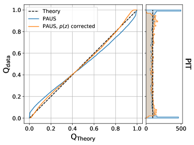
Figure 7: The Quantile-Quantile (QQ) plot, which tests the pdfs. This is plotted without and with a modified $p(z)$ that accounts for outliers. The right panel shows the distribution of cumulative pdf values (PIT), which should be uniform for an accurate pdf.

Several codes, including bpz, lephare, annz2 and skynet, produce pdfs. Depending on the code and data set, these can either be too broad or narrow (Tanaka et al., 2018). One approach to quantify the validity of the pdfs is to evaluate the cumulative of each $p(z)$ at the spectroscopic redshift. By convention in the photo-z community, we name this the probability integral transform (PIT Dawid, 1984). For a galaxy, this is defined as

$$\mathrm{PIT}\equiv\int_{0}^{z_{\mathrm{s}}}\mathrm{d}z\,p(z),$$ (17)

integrating the pdf from zero to the spectroscopic redshift ($z_{\mathrm{s}}$). If the pdfs are correctly estimated, then the PIT of a catalogue will form a uniform distribution. One way to present the PIT values is the Quantile-Quantile (QQ) plot. This shows for each quantile (x-axis) of the pdfs the fraction of the spectroscopic redshifts that is found there. Ideally the line would fall on the diagonal.

Figure 7 shows a Quantile-Quantile (QQ) plot for the PAUS photo-z. The line PAUS use the $p(z)$ directly from the photo-z code (no corrections). Here the line is lying below and above the diagonal at low and high quantiles, respectively. The distribution of PIT values (shown in the right panel) is quite uniform, but the very low and high quantiles have more galaxies than expected.

An assumption in the photo-z code is that the data are normally distributed (Eq. 4). Unfortunately, the PAUS data reduction has outliers, e.g. from scattered light and uncorrected cross-talk (Castander et al., in prep.; Serrano et al., in prep.). These translate into a different contribution to the $p(z)$ that is not accounted for in the pdf. The spikes are caused by photo-z outliers.

A simple model to correct the pdfs is by adding an additional uniformly distributed contribution, $p_{\mathrm{Outlier}}(z)$, to the distribution

$$p_{\mathrm{Corrected}}(z)=(1-\kappa)\,p(z)+\kappa\,p_{\mathrm{Outlier}}(z).$$ (18)

This represents the probability ($\kappa$) that a galaxy is found at a random location in the redshift fitting range. While there exist more complex ways of correcting the pdfs (Bordoloi, Lilly & Amara, 2010), this model is sufficient, since we only need to correct for catastrophic outliers.

Note that this correction will also depend on the photo-z quality cut. The ”PAUS, $p(z$) corrected” line in Figure 7 corresponds to setting $\kappa=0.13$ which achieves the smallest differences between the PIT distribution and the expected values for the 10 and 90 quantiles (peaks in Figure 7). This produces a pdf lying closer to the diagonal and corrects the PIT values on the edges.

6 Additional results

6.1 Redshift dependence

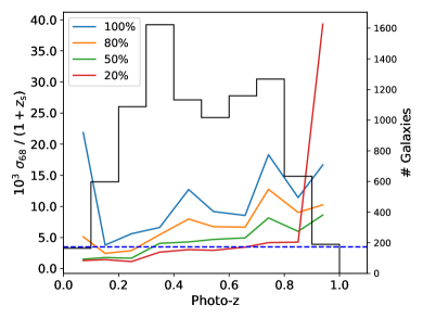
Figure 8: The redshift precision as a function of photometric redshift. The $i_{\mathrm{AB}}<22.5$ sample is split into 20 bins with equal number of galaxies, before being split again based on a quality cut (Qz). A horizontal line at $0.0035(1+z)$ shows the nominal PAUS target photo-z precision for a 50% quality cut. The black histogram shows the redshift distribution without quality cuts.

Figure 8 shows the photo-z scatter when splitting into redshift bins using the sample with $i_{\mathrm{AB}}<22.5$. Here the splitting is based on the photometric redshift, since this is how one will divide a sample without spectroscopic redshifts. There is a clear increase in the scatter, both with redshift and fraction of remaining galaxies. At redshift $\sim 0.28$ the $\text{H}_{\mathrm{\alpha}}$ line disappears from the PAUS wavelength range, leading to a photo-z degradation. A similar effect happens at $0.69\lesssim z\lesssim 0.73$, where OIII and $\text{H}_{\beta}$ leave. A horizontal line indicates the $0.0035(1+z)$ nominal target for 50% of the sample. While the photo-z performance degrades with redshift, the median redshift is low, so the sample average has a better redshift scatter than the figure might indicate. Furthermore, at high redshift the 20% line increases drastically. This is caused by outliers being scattered to high redshift, but having a narrow $p(z)$, leading to a good quality parameter.

6.2 Spatial variations

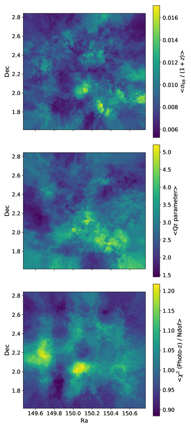
Figure 9: The spatial variations of photo-z precision, photo-z quality Qz and photo-z $\chi^{2}$ per degree of freedom (Ndof) within the COSMOS field. The images are generated by associating each pixel with the nearest 200 galaxies.

Figure 9 shows the spatial variations within the COSMOS field, with each subplot consisting of 100x100 pixels. There are too few galaxies ($\sim 10000$) in our sample to directly bin these based on position. Instead, we select the nearest 200 galaxies to each pixel using the tree-based algorithm in scipy. This roughly correspond to galaxies within 0.09 degrees. Based on this subsample we calculate different forms of statistics associated to the pixels.

The top panel (Fig. 9) shows the photo-z scatter. Note that the value of $\sigma_{68}/(1+z)$ is plotted without any quality cuts. Without quality cuts the absolute value is higher, but comparable to previous results for the full sample (Table 3). Some regions (see colourbar) have a higher scatter, which can be up to three times higher than in other regions. This can have implications for the science if not properly accounted for (Crocce et al., 2016).

In the middle panel the Qz parameter is shown. This form of diagnostics was previously used in (Martí et al., 2014b) using ODDS. The Qz parameter is the default parameter when applying a quality cut (see §5.5) and smaller values are better. As discussed (§5.5), cutting based on photo-z quality will introduce inhomogeneities. Last, the bottom panel shows the $\chi^{2}$ value when performing the photo-z fit. For each galaxy we use the minimum for all batches and redshifts. In this plot there is a clear pattern.

6.3 Emission line strength

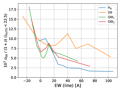
Figure 10: The photo-z precision as a function of the equivalent width (EW), for different emission lines. The x-axis shows the equivalent width for the narrow band where the emission line has the highest contribution.

Figure 10 shows $\sigma_{68}/(1+z)$ as a function of the equivalent width

$$\mathrm{EW}\equiv 100\mathrm{\AA}\,(f^{\text{Obs}}-f^{\text{Cont}})/f^{\text{Cont}},$$ (19)

where the narrow-bands are approximated with a 100Å wide top-hat filter and $f^{\text{Obs}}$ is the observed flux. The continuum ($f^{\text{Cont}}$) contribution is estimated by fitting the model used for the photo-z estimation at the true redshift. For higher emission line strengths, $\sigma_{68}/(1+z)$ decreases for all lines. This shows that emission lines are important for achieving high photo-z precision with PAUS. A negative emission line strength occurs when overestimating the continuum, e.g. by underestimating the extinction. It can also occur when the estimated flux in the emission line band is an outlier, e.g. from negative cross-talk. Statistically this yields high photo-z scatter. For the cases where this happens, we hope to solve this in future data reductions.

6.4 Galaxy subsamples

Luminous red galaxies (LRGs) constitute a useful sample for galaxy clustering studies. These galaxies are highly clustered, leading to a higher SNR in 2pt statistics (Eisenstein et al., 2001). They have proven to be an interesting component in the PAUS galaxy population at $z>0.4$ (Tortorelli et al., 2018). Furthermore, their pronounced 4000Å break leads to high photometric precision (Rozo et al., 2016) which makes them a useful sample for many studies, including BAO, galaxy-galaxy lensing, intrinsic alignments, to name a few (e.g. Tegmark et al., 2006; Joachimi et al., 2011; Mandelbaum et al., 2013; van Uitert et al., 2015; Elvin-Poole et al., 2018; Prat et al., 2018).

Figure 11 shows values of $\sigma_{68}/(1+z)$ for LRGs (solid), compared to the full sample (dashed). The x-axis shows the remaining fraction of galaxies selected by cutting on a quality parameter (Qz). The LRGs are selected by finding galaxies having a minimal $\chi^{2}$ for run #1 (Table 1). The LRG sample has a median $i_{\mathrm{AUTO}}$ of 21.5, which is brighter than the main sample, which has a median $i_{\mathrm{AUTO}}$ of 22.1. However, as these are intrinsically bright galaxies, this sample has a median photometric redshift of 0.69 and extends out to redshift 1.2. There are not enough spectra above $z>1$ to quantify the redshift precision, but we expect it to degrade significantly as the 4000Å break is not visible in PAUS beyond $z\sim 1.1$.

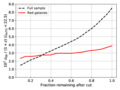
Figure 11: Photo-z precision ($\sigma_{68}/(1+z)$) for different fractions remaining on a quality cuts. One line shows the precision for the full sample (dashed), while the other for selected LRGs (solid). The LRGs are selected by having a minimal $\chi^{2}$ for ellipticl templates (run #1).

7 Conclusions

The PAUS survey is an extensive survey currently performed at the William Herschel Telescope. The novel aspect of the PAUCam instrument is the use of a 40 narrow-band filter set, spaced at 100Å intervals and covering 4500Å to 8500Å.

The goal is to combine the PAUS narrow bands with deeper broad bands over wide area weak lensing fields, such as the Canada-France Hawaii Telescope (CHFT/MegaCam) CFHTLenS Survey (Heymans et al., 2012), Kilo-Degree Survey (KiDS) (Kuijken et al., 2015) or Dark Energy Survey (DES) surveys (The Dark Energy Survey Collaboration, 2005).

In this paper we focus on COSMOS, which PAUS targeted for science verification, to quantify the performance of PAUS using actual data. In the case of the COSMOS field there are many existing measurements with different filters. Of particular interest are measurements presented in Laigle et al. (2016) with over 32 different broad and intermediate bands, that have been calibrated to measure the most accurate photo-z values to date.

As a test study, we combine the new PAUS images with only 6 of the COSMOS2015 broad bands representative of the CFHTLenS fields. These are: $u^{*}$ band data from the CFHTLenS and B, V, g, r, $i^{+}$ broad bands from Subaru, obtained in the COSMOS2015 Survey. Thus we have a total of 40+6 filters in PAUS, while COSMOS2015 used 32, but with wider wavelength coverage. The COSMOS2015 $i$-band catalogue is used to do forced photometry over the lower signal-to-noise (SNR) PAUS narrow band images.

One of the challenges for the PAUS photo-z code is the combination of a few (six) high SNR bands with many (40) narrow bands with low SNR. Another challenge is the relative calibration of these surveys, which is validated in §5.2. This paper presents the first PAUS photometric redshifts on the COSMOS field to magnitudes $i$-band $<22.5$. The photometric redshifts are estimated by a new photo-z code, bcnz2, presented in §4. This code is similar to eazy (Brammer, van Dokkum & Coppi, 2008), which computes a linear combination of SED templates. However, it has a different treatment of emission lines and extinction.

Figure 3 is the main result of this paper. The panels show the preliminary PAUS photo-z accuracy $\sigma_{68}$ and the outlier fraction as a function of cumulative $i$-band magnitude. These preliminary result already match the expected photo-z precision of $\sigma_{68}/(1+z)\simeq 0.0035$ for $i_{\mathrm{AB}}<22.5$ and a best 50% photometric redshift quality cut. The results are also significantly better, for the same objects, than the state-of-the-art. COSMOS2015 photo-z results are based on measurements with a much larger wavelength coverage and better signal-to-noise ratio, but not as good wavelength resolution as PAUS.

We also find better than expected photo-z accuracy (comparable to spectroscopy) for high SNR measurements, for emission line galaxies and for colour-selected subsamples. These results demonstrate the feasibility of the PAUS programme, but they are neither final nor optimal. When we split the sample in differential magnitude bins or look at the consistency of the cumulative redshift probabilities (pdf), we find evidence for an excess of outliers that require further optimisation and investigation. We are also working on several improvements to our processing and photo-z codes. We are therefore hopeful to achieve better performance and present new science applications in the near future.

Appendix A The bcnz photo-z code

A.1 Minimisation algorithm

The minimisation of the $\chi^{2}$ (Eq. 3) has a closed form solution. However, this includes solutions where some of the amplitudes (${\bm{\alpha}}$) are negative. These are undesirable because they lead to unphysical solutions. Applying a negative amplitude to some SEDs would cancel out features of the data, leading to worse redshift accuracy. We therefore require the amplitudes to be positive.

To minimize the $\chi^{2}$, we used a method for non-negative quadratic programming, given in Sha et al. (2007). The minimisation uses an iterative algorithm, which defines

$$A_{xy}\equiv\sum_{i}\frac{f_{i}^{x}f_{i}^{y}}{\sigma_{i}^{2}},\quad b_{x}\equiv\sum_{i}\frac{f_{i}^{x}\tilde{f}_{i}}{\sigma_{i}^{2}}$$ (20)

for templates $x,y$, where the summations are over the bands denoted by $i$. If ${\bm{\alpha}}$ is the set of amplitudes at a certain step, the updated amplitudes $\bar{\bm{\alpha}}$ at the next step are then

$$m_{x}=\frac{b_{x}}{\sum_{xy}A_{xy}{\bm{\alpha}}_{y}},\quad\bar{{\bm{\alpha}}}_{x}=m_{x}{\bm{\alpha}}_{x},$$ (21)

where the summation in the determination could use a matrix product. In the implementation the minimum is estimated at the same time for a set of galaxies, for all the different redshift bins.

A.2 Language

The bcnz2 code is mainly written in python (van Rossum, 1995), but with the core algorithm in julia (Bezanson et al., 2017). The python language is widely used in the astronomical community, partly because of being a high-level language, allowing to code up difficult problems in fewer lines. In particular, the bcnz2 code relies heavily on pandas (McKinney, 2010) and xarray (Hoyer & Hamman, 2017).

Python code written in the style of c and fortran, relying on loops, is slow. For numerical tasks, one should either use fast building blocks as matrix operations or call a library written in another language. Alternatively one can use numba (Lam, Pitrou & Seibert, 2015), a just-in-time compiler converting math intensive Python to machine instructions. Adding a single line numba decorator (@numba.jit) reduced the runtime to about 2/3 of the original value. Other alternatives include cython (Behnel et al., 2011), c++ (Stroustrup, 2000) or julia. In the end we decided on julia, since the code was readable and executed fast.

A.3 Infrastructure

Running the photo-z code can be time consuming. Having access to an environment with multiple CPUs allows us to calculate the photo-z faster, allowing for more iterations. The bcnz2 code is integrated within the Apache Spark cluster (Zaharia et al., 2010) running at Port d’Informació Científica (PIC). This platform is also used for CosmoHub (Carretero et al., 2017). Spark is suitable for programs where the calculations can be split into independent parts, with the result being combined at the end (map-reduce). For the photo-z we split into sets of galaxies. Users can either run bcnz2 locally or remotely run the code at PIC.

A.4 Convergence

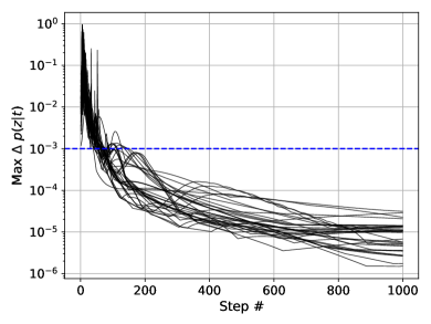
Figure 12: A convergence test, showing the maximum absolute change in p(z) for all redshifts for a set for 10 galaxies. On the x-axis is the number of steps in the iterative minimisation, while each line corresponds to a photo-z run (Table 1).

The basic minimisation algorithm is made to minimise the $\chi^{2}$ separately at each redshift, and is proven to reach convergence (Sha et al., 2007), but the question is how fast convergence is reached. That is important when running the photo-z, since the minimisation is the most time consuming part.

Figure 12 shows a benchmark for the convergence. On the x-axis is the iteration step, while the y-axis shows the maximum absolute change in $p(z)$. The maximum absolute change in $p(z)$ is estimated between two iteraction and selects the redshift with maximum change for any of the galaxies in the batch of 10 galaxies.

This quantity was chosen, since it relates more directly to the error we want to minimise. We first attempted to study the convergence looking at the model amplitude (${\bm{\alpha}}$) changes. This had the problem of some amplitudes being unconstrained, e.g. when an emission line does not enter into any of the bands. Further, focusing on the $\chi^{2}$ value is also problematic, since changes to high $\chi^{2}$ values are less important for the final result. Hence we ended up focusing on the $p(z)$ values.

In this plot each line corresponds to one of the 45 photo-z runs (Table 1). Here we selected 10 galaxies, which correspond to how many are usually being run together. For each step we estimated the $p(z)$ for that photo-z run. Note that most runs do not correspond to the optimal. The distribution will therefore be broader and the convergence slightly slower.

While the $\chi^{2}$ is proven to converge uniformly, this is not the case for the $p(z)$. During the minimisation, the $\chi^{2}$ at different redshift grid values will converge faster to the correct value. In practice, we find many cases where the $p(z)$ peak position changes from one redshift to another after some iterations. This explains why some of the lines increase within the first iterations ($<200$). A horizontal line marks a very stringent requirement on the convergence. By default we run all batches with 1000 iterations, although 500 should be sufficient.

Appendix B Miscellaneous

Spectroscopic completeness:

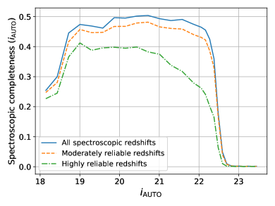
Figure 13: The completeness in the zCOSMOS DR3 bright sample. Here the completeness is the fraction of galaxies with spec-z compared to the full COSMOS sample for different magnitude bins. Three lines show the full sample (solid), when selecting moderately secure redshifts (dashed) [classes: 3.x, 4.x, 2.5, 2.4, 1.5, 9.5, 9.4, 9.3, 18.5, 18.3] and highly secure redshifts (dash-dotted) [classes: 3.x, 4.x].

Figure 13 shows the spectroscopic redshift completeness as a function of $i_{\mathrm{AUTO}}$, the SExtractor’s AUTO magnitude (MAG_AUTO) in the $i$-band. zCOSMOS DR3 bright data have a 44% completeness for $i_{\mathrm{{AUTO}}}\leq 22.5$, which reduces to 28% after imposing the spectra to be highly reliable. For this paper we use the highly reliable redshifts (3.x, 4.x), as suggested in zCOSMOS DR3. The spectroscopic completeness of our reference has to be kept in mind when presenting the result as a function of magnitude.

Broad band transmission curves:

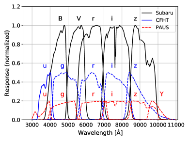
Figure 14: The Subaru, CFHT and PAUS broad band throughputs, which for improving the visualisation are each normalised to 1.0, 0.5 and 0.2, respectively. Solid lines mark filters which are used in the photo-z run, while dashed filters are only included as a reference.

Figure 14 shows the broad band transmission curves. PAUS science cases use external broad band datasets as reference catalogues, for which we produce precise photo-zs. Therefore PAUCam’s own broad bands are not used currently in PAUS, but are included for reference. The transmission for broad bands corresponding to Subaru and the Canadian-France Hawaii Telescope camera are shown.

Photo-z scatter

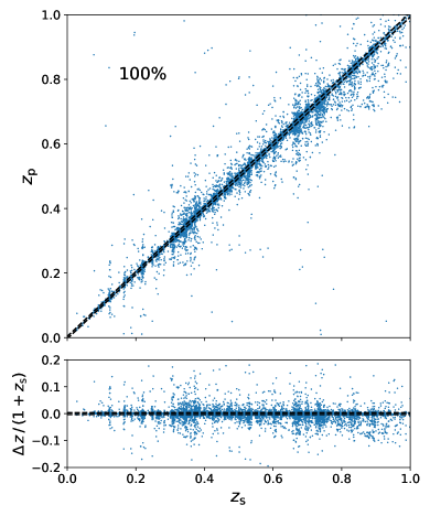
Figure 15: The photo-z performance without quality cuts as a function of spectroscopic redshift ($z_{\mathrm{s}}$). The y-axis top panel shows the photometric redshift ($z_{\mathrm{p}}$), while the bottom panel shows the scatter $(z_{\mathrm{p}}-z_{\mathrm{s}})/(1+z_{\mathrm{s}})$. The two lines mark the $1-\sigma$ limits for the 0.0035(1+z) target precision.

Figure 15 shows the photo-z scatter plot, corresponding to the data in Figure 3 and 16. Here the result is shown for the full sample (no quality cuts).

Differential magnitude bins:

Figure 16 shows the same results as Figure 3, but in differential, instead of cumulative magnitude bins. Here we can see more clearly the degradation of both accuracy and number of outliers at the faint end of the sample. There is an excess of outliers which arise from both the lower signal-to-noise ratio and the non-optimal treatment of data and photo-z code in this regime. These are preliminary results and we are implementing new methods to improve this performance.

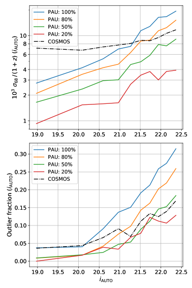
Figure 16: Same as Figure 3, but showing the differential performance as a function of magnitude.

Appendix C Galaxy internal extinction

There are multiple contributions to the extinction, both from the Milky Way and internally in the galaxies we observe. The Galactic extinction is corrected for by the calibration procedure described in Castander et al. (in prep.). Internal galaxy extinction varies from galaxy to galaxy and needs to be included in the modelling of each galaxy SED.

Galaxy internal extinction results from dust scattering light, reducing the light transmitted in the direction of the observer. Let $F_{i}(\lambda)$ be the intrinsic galaxy spectrum and $F_{o}(\lambda)$ be the observable spectrum after extinction. Then

$$F_{o}(\lambda)=F_{i}(\lambda){10}^{-0.4E(B-V)k(\lambda)}$$ (22)

relates the two. Here the $E(B-V)$ parameter measures the magnitude difference in the B and V bands. As follows, the $k(\lambda)$ wavelength dependent function is determined through observations.

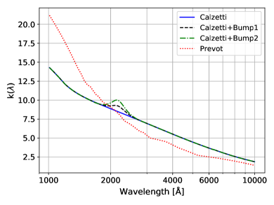
Figure 17: The internal extinction curves. The Calzetti extinction curve (solid) is applied to starburst galaxies. Two extinction laws (dashed and dot-dashed) add an additional contribution at 2175Å. The Prevot extinction (dotted) is applied to spiral galaxies.

Figure 17 shows the wavelength dependence of the extinction laws used. Multiple relations exist in the literature. One commonly used is the extinction law of Calzetti et al. (2000), which is fitted to observed starburst galaxies. The photo-z code uses the Calzetti et al. (2000) extinction law for starburst templates.

A characteristic feature in the extinction is the 2175Å bump (Stecher & Donn, 1965). Polycyclic aromatic hydrocarbon (PAH) molecular transitions have been suggested as an explanation, but the origin is still debated (Xiang, Li & Zhong, 2011). This feature is left out of the Calzetti relation, since their starburst galaxy spectra did not show a prominent feature around 2175Å (Calzetti, Kinney & Storchi-Bergmann, 1994).

In Fitzpatrick & Massa (1986, 2007) the authors parameterised the 2175Å bump with a Drude profile

$$D(x,x_{0},\gamma)=\frac{x^{2}}{{(x^{2}-x_{0}^{2})}^{2}+x^{2}\gamma^{2}},$$ (23)

which gives an analytical expression for the 2175Å bump. The COSMOS2015 paper used the Calzetti extinction law, including this additional contribution. This paper uses their tabulated values. Two different versions exist, one with double strengths of the 2175Å feature. When running with the Calzetti law, we also fit with these two modified versions. The Prevot extinction was measured in the Small Magellanic Cloud (SMC) (Prevot et al., 1984). This extinction law is commonly applied for spiral galaxies, including in COSMOS2015. By default we do not include the Prevot extinction, but have tested applying it to spiral templates. This significanly reduced the photo-z precision, hence we do not include the Prevot extinction.

References

- Alarcon, Eriksen & Gaztanaga (2018) Alarcon A., Eriksen M., Gaztanaga E., 2018, MNRAS, 473, 1444
- Allen (1976) Allen C. W., 1976, Astrophysical Quantities
- Arnouts & Ilbert (2011) Arnouts S., Ilbert O., 2011, LePHARE: Photometric Analysis for Redshift Estimate. Astrophysics Source Code Library
- Asorey et al. (2016) Asorey J., Carrasco Kind M., Sevilla-Noarbe I., Brunner R. J., Thaler J., 2016, MNRAS, 459, 1293
- Baldwin, Phillips & Terlevich (1981) Baldwin J. A., Phillips M. M., Terlevich R., 1981, PASP, 93, 5
- Beck et al. (2016) Beck R., Dobos L., Yip C.-W., Szalay A. S., Csabai I., 2016, MNRAS, 457, 362
- Behnel et al. (2011) Behnel S., Bradshaw R., Citro C., Dalcin L., Seljebotn D., Smith K., 2011, Computing in Science Engineering, 13, 31
- Benítez (2000) Benítez N., 2000, ApJ, 536, 571
- Benítez et al. (2009) Benítez N. et al., 2009, ApJ, 691, 241
- Bertin (2011) Bertin E., 2011, in Astronomical Society of the Pacific Conference Series, Vol. 442, Astronomical Data Analysis Software and Systems XX, Evans I. N., Accomazzi A., Mink D. J., Rots A. H., eds., p. 435
- Bertin & Arnouts (1996) Bertin E., Arnouts S., 1996, A&AS, 117, 393
- Bezanson et al. (2017) Bezanson J., Edelman A., Karpinski S., Shah V. B., 2017, SIAM Review, 59, 65
- Bonnett (2015) Bonnett C., 2015, MNRAS, 449, 1043
- Bordoloi, Lilly & Amara (2010) Bordoloi R., Lilly S. J., Amara A., 2010, MNRAS, 406, 881
- Brammer, van Dokkum & Coppi (2008) Brammer G. B., van Dokkum P. G., Coppi P., 2008, ApJ, 686, 1503
- Bruzual & Charlot (2003) Bruzual G., Charlot S., 2003, MNRAS, 344, 1000
- Cabayol et al. (2018) Cabayol L. et al., 2018, preprint(ArXiv:1806.08545)
- Calzetti et al. (2000) Calzetti D., Armus L., Bohlin R. C., Kinney A. L., Koornneef J., Storchi-Bergmann T., 2000, ApJ, 533, 682
- Calzetti, Kinney & Storchi-Bergmann (1994) Calzetti D., Kinney A. L., Storchi-Bergmann T., 1994, ApJ, 429, 582
- Carretero et al. (2017) Carretero J., et al., 2017, PoS, EPS-HEP2017, 488
- Casas et al. (2016) Casas R. et al., 2016, in Proc.SPIE, Vol. 9908, pp. 9908 – 9908 – 12
- Casas et al. (2014) Casas R., Cardiel-Sas L., Castander F., Jiménez J., de Vicente J., 2014, in Proc.SPIE, Vol. 9147, pp. 9147 – 9147 – 8
- Castander et al. (in prep.) Castander F., Eriksen M., Serrano S., et al., in prep.
- Castander & et al. (2012) Castander F., et al., 2012, in Proc.SPIE, Vol. 8446, pp. 8446 – 8446 – 9
- Catelan, Kamionkowski & Blandford (2001) Catelan P., Kamionkowski M., Blandford R. D., 2001, MNRAS, 320, L7
- Crocce et al. (2016) Crocce M. et al., 2016, MNRAS, 455, 4301
- Croft & Metzler (2000) Croft R. A. C., Metzler C. A., 2000, ApJ, 545, 561
- Davis et al. (2003) Davis M. et al., 2003, in Proc. SPIE, Vol. 4834, Discoveries and Research Prospects from 6- to 10-Meter-Class Telescopes II, Guhathakurta P., ed., pp. 161–172
- Dawid (1984) Dawid A. P., 1984, Journal of the Royal Statistical Society. Series A (General), 147, 278
- De Vicente, Sánchez & Sevilla-Noarbe (2016) De Vicente J., Sánchez E., Sevilla-Noarbe I., 2016, MNRAS, 459, 3078
- Driver et al. (2009) Driver S. P. et al., 2009, Astronomy and Geophysics, 50, 5.12
- Eisenstein et al. (2001) Eisenstein D. J. et al., 2001, AJ, 122, 2267
- Elvin-Poole et al. (2018) Elvin-Poole J. et al., 2018, Phys. Rev. D, 98, 042006
- Eriksen & Gaztañaga (2015) Eriksen M., Gaztañaga E., 2015, MNRAS, 452, 2168
- Fitzpatrick & Massa (1986) Fitzpatrick E. L., Massa D., 1986, ApJ, 307, 286
- Fitzpatrick & Massa (2007) Fitzpatrick E. L., Massa D., 2007, ApJ, 663, 320
- Gaia Collaboration (2016) Gaia Collaboration, 2016, A&A, 595, A2
- Gaztañaga, Cabré & Hui (2009) Gaztañaga E., Cabré A., Hui L., 2009, MNRAS, 399, 1663
- Gaztañaga et al. (2012) Gaztañaga E., Eriksen M., Crocce M., Castander F. J., Fosalba P., Marti P., Miquel R., Cabré A., 2012, MNRAS, 422, 2904
- Heavens, Refregier & Heymans (2000) Heavens A., Refregier A., Heymans C., 2000, MNRAS, 319, 649
- Heymans et al. (2012) Heymans C. et al., 2012, MNRAS, 427, 146
- Hildebrandt et al. (2012) Hildebrandt H. et al., 2012, MNRAS, 421, 2355
- Hirata & Seljak (2004) Hirata C. M., Seljak U., 2004, Phys. Rev. D, 70, 063526
- Hogg et al. (2002) Hogg D. W., Baldry I. K., Blanton M. R., Eisenstein D. J., 2002, preprint(arXiv:astro-ph/0210394)
- Hoyer & Hamman (2017) Hoyer S., Hamman J., 2017, Journal of Open Research Software, 5
- Hoyle et al. (2018) Hoyle B. et al., 2018, MNRAS, 478, 592
- Ilbert et al. (2009) Ilbert O. et al., 2009, ApJ, 690, 1236
- Ilbert et al. (2013) Ilbert O. et al., 2013, A&A, 556, A55
- Joachimi et al. (2015) Joachimi B. et al., 2015, Space Sci. Rev., 193, 1
- Joachimi et al. (2011) Joachimi B., Mandelbaum R., Abdalla F. B., Bridle S. L., 2011, A&A, 527, A26
- Jouvel et al. (2014) Jouvel S., Abdalla F. B., Kirk D., Lahav O., Lin H., Annis J., Kron R., Frieman J. A., 2014, MNRAS, 438, 2218
- Knobel et al. (2012) Knobel C. et al., 2012, ApJ, 753, 121
- Koekemoer et al. (2007) Koekemoer A. M. et al., 2007, ApJS, 172, 196
- Kuijken et al. (2015) Kuijken K. et al., 2015, MNRAS, 454, 3500
- Laigle et al. (2016) Laigle C. et al., 2016, ApJS, 224, 24
- Lam, Pitrou & Seibert (2015) Lam S. K., Pitrou A., Seibert S., 2015, in Proceedings of the Second Workshop on the LLVM Compiler Infrastructure in HPC, LLVM ’15, ACM, New York, NY, USA, pp. 7:1–7:6
- Laureijs et al. (2011) Laureijs R. et al., 2011, preprint(arXiv:1110.3193)
- Leauthaud et al. (2007) Leauthaud A. et al., 2007, ApJS, 172, 219
- Lilly et al. (2009) Lilly S. J. et al., 2009, ApJS, 184, 218
- Lilly et al. (2007) Lilly S. J. et al., 2007, ApJS, 172, 70
- LSST Science Collaboration (2009) LSST Science Collaboration, 2009, preprint(arXiv:0912.0201)
- Madrid et al. (2010) Madrid F. et al., 2010, in Proc.SPIE, Vol. 7735, pp. 7735 – 7735 – 7
- Mandelbaum et al. (2013) Mandelbaum R., Slosar A., Baldauf T., Seljak U., Hirata C. M., Nakajima R., Reyes R., Smith R. E., 2013, MNRAS, 432, 1544
- Martí et al. (2014a) Martí P., Miquel R., Bauer A., Gaztañaga E., 2014a, MNRAS, 437, 3490
- Martí et al. (2014b) Martí P., Miquel R., Castander F. J., Gaztañaga E., Eriksen M., Sánchez C., 2014b, MNRAS, 442, 92
- McKinney (2010) McKinney W., 2010, in Proceedings of the 9th Python in Science Conference, van der Walt S., Millman J., eds., pp. 51 – 56
- Moles et al. (2008) Moles M. et al., 2008, AJ, 136, 1325
- Molino et al. (2014) Molino A. et al., 2014, MNRAS, 441, 2891
- Nakajima et al. (2012) Nakajima R., Mandelbaum R., Seljak U., Cohn J. D., Reyes R., Cool R., 2012, MNRAS, 420, 3240
- Padilla et al. (in prep.) Padilla C., Castander F., Fernandez E., et al., in prep.
- Pickles (1998) Pickles A. J., 1998, PASP, 110, 863
- Planck Collaboration et al. (2016) Planck Collaboration et al., 2016, A&A, 594, A13
- Prat et al. (2018) Prat J. et al., 2018, Phys. Rev. D, 98, 042005
- Prevot et al. (1984) Prevot M. L., Lequeux J., Maurice E., Prevot L., Rocca-Volmerange B., 1984, A&A, 132, 389
- Rozo et al. (2016) Rozo E. et al., 2016, MNRAS, 461, 1431
- Sadeh, Abdalla & Lahav (2016) Sadeh I., Abdalla F. B., Lahav O., 2016, PASP, 128, 104502
- Sargent et al. (2007) Sargent M. T. et al., 2007, ApJS, 172, 434
- Schlegel, Finkbeiner & Davis (1998) Schlegel D. J., Finkbeiner D. P., Davis M., 1998, ApJ, 500, 525
- Serrano et al. (in prep.) Serrano S., Castander F., Fernandez E., et al., in prep.
- Serrano et al. (in prep.) Serrano S., Gaztañaga E., Eriksen M., Castander F., in prep.
- Sha et al. (2007) Sha F., Lin Y., Saul L. K., Lee D. D., 2007, Neural Comput., 19, 2004
- Smith et al. (2002) Smith J. A. et al., 2002, AJ, 123, 2121
- Spergel et al. (2015) Spergel D. et al., 2015, preprint(arXiv:1503.03757)
- Stecher & Donn (1965) Stecher T. P., Donn B., 1965, ApJ, 142, 1681
- Strauss et al. (2002) Strauss M. A. et al., 2002, AJ, 124, 1810
- Stroustrup (2000) Stroustrup B., 2000, The C++ Programming Language, 3rd edn. Addison-Wesley Longman Publishing Co., Inc., Boston, MA, USA
- Tanaka et al. (2018) Tanaka M. et al., 2018, PASJ, 70, S9
- Tanaka et al. (2004) Tanaka M., Goto T., Okamura S., Shimasaku K., Brinkmann J., 2004, The Astronomical Journal, 128, 2677
- Taniguchi et al. (2015) Taniguchi Y. et al., 2015, PASJ, 67, 104
- Tegmark et al. (2006) Tegmark M. et al., 2006, Phys. Rev. D, 74, 123507
- The Dark Energy Survey Collaboration (2005) The Dark Energy Survey Collaboration, 2005, preprint (ArXiv:astro-ph/0510346)
- Tonello et al. (in prep.) Tonello N., Tallada P., Serrano S., et al., in prep.
- Tortorelli et al. (2018) Tortorelli L. et al., 2018, preprint(ArXiv:1805.05340)
- Troxel & Ishak (2015) Troxel M. A., Ishak M., 2015, Phys. Rep., 558, 1
- van Dokkum (2001) van Dokkum P. G., 2001, PASP, 113, 1420
- van Rossum (1995) van Rossum G., 1995, Python tutorial, Technical Report CS-R9526. Tech. rep., Centrum voor Wiskunde en Informatica (CWI), Amsterdam
- van Uitert et al. (2015) van Uitert E., Cacciato M., Hoekstra H., Herbonnet R., 2015, A&A, 579, A26
- Weinberg et al. (2013) Weinberg D. H., Mortonson M. J., Eisenstein D. J., Hirata C., Riess A. G., Rozo E., 2013, Phys. Rep., 530, 87
- Xiang, Li & Zhong (2011) Xiang F. Y., Li A., Zhong J. X., 2011, ApJ, 733, 91
- Zaharia et al. (2010) Zaharia M., Chowdhury M., Franklin M. J., Shenker S., Stoica I., 2010, in Proceedings of the 2Nd USENIX Conference on Hot Topics in Cloud Computing, HotCloud’10, USENIX Association, Berkeley, CA, USA, pp. 10–10