Effects of rotation and magnetic field on the revival of a stalled shock in supernova explosions

Abstract

We investigate axisymmetric steady solutions of (magneto)hydrodynamics equations that describe approximately accretion flows through a standing shock wave and discuss the effects of rotation and magnetic field on the revival of the stalled shock wave in supernova explosions. We develop a new powerful numerical method to calculate the 2-dimensional (2D) steady accretion flows self-consistently. We first confirm the results of preceding papers that there is a critical luminosity of irradiating neutrinos, above which there exists no steady solution in spherical models. If a collapsing star has rotation and/or magnetic field, the accretion flows are no longer spherical owing to the centrifugal force and/or Lorentz force and the critical luminosity is modified. In fact we find that the critical luminosity is reduced by about $50\%$ – $70\%$ for rapid rotations and about $20\%$ – $50\%$ for strong toroidal magnetic fields, depending on the mass accretion rate. These results may be also interpreted as an existence of the critical specific angular momentum or critical magnetic field, above which there exists no steady solution and the standing shock wave will revive for a given combination of mass accretion rate and neutrino luminosity.

1 Introduction

Core-collapse supernovae (CCSNe) play important roles in various fields of astrophysics such as the star formation, galactic evolution and the acceleration of cosmic-ray through their nucleosynthesis, energetic shock waves and high luminosities. The large gravitational energy liberated in the collapse makes CCSNe promising sites for the emissions of neutrinos and gravitational waves as well as heavy elements. The understanding of the physical processes in and the mechanism of CCSNe is important for the development of multi-messenger astronomy.

CCSNe commence with the gravitational collapse of the core of massive stars at the ends of their lives. When the central density reaches the nuclear saturation density, core bounce occurs and a shock wave is generated. As it propagates outward, the shock loses energy via photo-dissociations of nuclei and neutrino cooling and is eventually stagnated inside the core by the ram pressure of accreting matter in addition to these energy losses. The stalled shock wave should be revived somehow to produce a successful explosion. It is widely expected that it will be re-energized by the irradiation of matter behind it by neutrinos diffusing out of a proto-neutron star (PNS) (Wilson, 1985). This neutrino heating scenario is currently the most favored mechanism of CCSNe (Janka et al., 2012; Kotake et al., 2012; Burrows, 2013; Foglizzo et al., 2015; Müller, 2016; Burrows et al., 2018 for recent reviews).

Intensive and extensive efforts in numerical simulations have revealed so far that no successful explosion obtains in spherical symmetry (e.g. Liebendörfer et al., 2001, 2005; Rampp & Janka, 2002; Sumiyoshi et al., 2005) and multi-dimensional effects are crucially important (Burrows et al. 2006; Marek & Janka 2009; Bruenn et al. 2009; Suwa et al. 2010; Müller et al. 2012; Takiwaki et al. 2012; Hanke et al. 2013; Murphy et al. 2013; Couch 2013; Couch & Ott 2013; Lentz et al. 2015; Nakamura et al. 2015; Melson et al. 2015; Roberts et al. 2016; Bruenn et al. 2016; O’Connor & Couch 2018). Important effects among them are rotation (Fryer & Heger 2000; Kotake et al. 2003; Thompson et al. 2005; Marek & Janka 2009; Iwakami et al. 2014a; Nakamura et al. 2014; Takiwaki et al. 2016; Summa et al. 2018), magnetic field (Akiyama et al. 2003; Yamada & Sawai 2004; Kotake et al. 2004; Sawai et al. 2005; Obergaulinger et al. 2006; Burrows et al. 2007; Takiwaki et al. 2009; Sawai & Yamada 2014; Obergaulinger et al. 2014; Mösta et al. 2015; Sawai & Yamada 2016; Obergaulinger et al. 2018), non-spherical structures of the progenitor (Couch & Ott 2013; Takahashi & Yamada 2014; Couch et al. 2015; Takahashi et al. 2016), turbulence (Murphy & Burrows 2008; Murphy & Meakin 2011; Murphy et al. 2013; Couch & Ott 2015; Mabanta & Murphy 2018), (magneto)hyrdodynamical instabilities (Blondin et al. 2003; Scheck et al. 2006; Blondin & Mezzacappa 2007; Iwakami et al. 2008; Guilet et al. 2010; Wongwathanarat et al. 2010; Takiwaki et al. 2014; Fernández et al. 2014; Fernández 2015), general relativistic gravity (Dimmelmeier et al. 2002; Shibata & Sekiguchi 2004, 2005, Müller et al. 2012; Ott et al. 2012; Kuroda et al. 2012, 2016) and neutrino transport (Nagakura et al. 2014; Dolence et al. 2015; Pan et al. 2016; Nagakura et al. 2017, 2018). It is true that large-scale dynamical simulations have played a crucial role in the recent progresses in our understanding of these ingredients, but we believe that a more phenomenological approach that employs toy models still plays an indispensable and complementary role to understand each effect more deeply.

Burrows & Goshy (1993) took such an approach and introduce the concept of the critical neutrino luminosity. They approximated the accretion flows after the shock wave is stagnated with spherical steady solutions with constant mass accretion rates of the hydrodynamics (HD) equations that incorporate neutrino heating of matter; they found then that for a given mass accretion rate, there is a critical neutrino luminosity, above which no steady solution exists; they surmised that the revival of the stalled shock wave should occur there. The existence of such a critical neutrino luminosity was confirmed both in similar phenomenological methods (Yamasaki & Yamada, 2005, 2007; Keshet & Balberg 2012; Murphy & Dolence 2017) and in numerical simulations (Janka & Mueller, 1996; Ohnishi et al. 2006; Iwakami et al. 2008; Murphy & Burrows 2008; Nordhaus et al. 2010; Iwakami et al. 2014b, a; Suwa et al. 2016).

For examples in the phenomenological models, Pejcha & Thompson (2012) contended that the ante-sonic condition for the ratio of the sound velocity to the escape velocity is an important diagnostic for explosion. (see also Raives et al. 2018). Nagakura et al. (2013) argued, on the other hand, that there is a critical fluctuation for a given accretion flow, above which the shock wave can sustain its outward propagation once launched. Gabay et al. (2015) applied a phase-space analysis to the shock acceleration in the shock radius and shock velocity plane. More recently Murphy & Dolence (2017) contended that five parameters (mass accretion rate, neutrino luminosity, neutrino temperature, PNS mass and radius) instead of two (mass accretion rate and neutrino luminosity alone) are more appropriate in considering the condition for explosion. They also derived a diagnostic dimensionless quantity $\Psi$ from the integrability condition, which roughly measures the balance between pressure and gravity. It should be stressed here that all these conditions are based on the analysis of spherical accretion flows and should be modified if the background flow is non-spherical.

In fact, it was shown that the critical luminosity is lowered by rotation both in the phenomenological method (Yamasaki & Yamada, 2005) and dynamical simulations (Murphy & Burrows, 2008; Nordhaus et al. 2010; Hanke et al. 2013; Couch 2013; Iwakami et al., 2014b, a). Yamasaki & Yamada (2005) extended their spherically-symmetric, steady accretion-flow to axisymmetric ones, taking rotation into account consistently. They showed that the accretion flows become non-radial in the presence of rotation and the critical luminosity is lowered. Iwakami et al. (2014a), on the other hand, performed 3-dimensional (3D) dynamical simulations of rotational accretions and obtained similar results: the critical luminosity is lowered by rapid rotation and there is a critical value of specific angular momentum, above which the shock wave is revived, for a given combination of mass accretion rate and neutrino luminosity. This implies that an explosion may be triggered by rapid rotation even if the neutrino luminosity is sub-critical without rotation.

It is emphasized here that Yamasaki & Yamada (2005) is the only one that has so far taken the phenomenological approach to the non-spherical accretion flows. This is in sharp contrast to the fact that there have been many numerical simulations that are meant to address the issue (Janka & Mueller, 1996; Ohnishi et al. 2006; Iwakami et al. 2008; Murphy & Burrows 2008; Nordhaus et al. 2010; Hanke et al. 2013; Iwakami et al. 2014b, a; Suwa et al. 2016). The reason for this is probably the difficulty to obtain numerically non-spherical steady solutions of the HD equations. Even in Yamasaki & Yamada (2005), the number of solutions was not large. Not to mentions, there has been no attempt to incorporate magnetic field in such approaches.

In this paper, we develop a new numerical scheme to numerically obtain axisymmetric steady solutions of HD and magnetohydrodynamics (MHD) equations that describe self-consistently non-spherical post-shock accretion flows in the presence of rotation and/or magnetic field. Based on these solutions we study the effects of rotation and magnetic field on the critical neutrino luminosity systematically. This paper is organized as follows. In Sec. 2 we formulate the problem and give the basic equations to be solved. We then explain our new numerical method. In Sec. 3 we present numerical solutions and the critical luminosities obtained from them. Finally we give some discussions and summarize this paper in Sec. 4.

2 Formulations

2.1 Assumptions and basic equations

After the shock stalls, the mass accretion rate and neutrino luminosity change slowly and the post-shock accretion flows may be approximated as steady states with constant mass accretion rates and neutrino luminosities (Burrows & Goshy 1993; Yamasaki & Yamada 2005). We make the following assumptions to construct idealized models in this paper.

1. The equatorial symmetry is assumed in addition to the stationary ($\partial/\partial t=0$) and axisymmetry ($\partial/\partial\varphi=0$).

2. We ignore both viscosity and magnetic resistivity and consider only ideal HD or MHD equations.

3. We consider the accretion flows only in the domain between the stalled shock wave and the neutrino sphere and impose the outer and inner boundary conditions there.

4. The PNS is treated as a point mass with $1.3~{}\mathrm{M_{\odot}}$. Only its Newtonian gravitational forces are considered and the self-gravity of accreting matter is ignored for simplicity.

5. We neglect the neutrino transfer again for simplicity and the luminosity and energy spectrum of neutrinos are assumed to be constant in radius (see Equations 4 and 5).

6. A simplified equation of state (EOS) that neglects the photo-dissociations of nuclei is adopted and the convection is not taken into account.

Under these assumptions, the basic equations are given as

$$\frac{1}{r^{2}} \frac{\partial}{\partial r}\left(r^{2}\rho u_{r}\right)+\frac{1}{r\sin\theta}\frac{\partial}{\partial\theta}\left(\sin\theta\rho u_{\theta}\right)=0,$$ (1a)

$$u_{r} \frac{\partial u_{r}}{\partial r}+\frac{u_{\theta}}{r}\frac{\partial u_{r}}{\partial\theta}-\frac{u_{\theta}^{2}+u_{\varphi}^{2}}{r}=-\frac{1}{\rho}\frac{\partial p}{\partial r}-\frac{GM}{r^{2}}$$

$$-\frac{1}{4\pi\rho}\Bigg{[}B_{\theta}\frac{\partial B_{\theta}}{\partial r}+B_{\varphi}\frac{\partial B_{\varphi}}{\partial r}+\frac{B_{\theta}^{2}+B_{\varphi}^{2}}{r}\Bigg{]},$$ (1b)

$$u_{r} \frac{\partial u_{\theta}}{\partial r}+\frac{u_{\theta}}{r}\frac{\partial u_{\theta}}{\partial\theta}+\frac{u_{r}u_{\theta}}{r}-\frac{u_{\varphi}^{2}\cot\theta}{r}=-\frac{1}{\rho r}\frac{\partial p}{\partial\theta}$$

$$+\frac{1}{4\pi\rho}\Bigg{[}B_{r}\frac{\partial B_{\theta}}{\partial r}-\frac{B_{r}}{r}\frac{\partial B_{r}}{\partial\theta}$$

$$-\frac{B_{\varphi}}{r}\frac{\partial B_{\varphi}}{\partial\theta}+\frac{B_{r}B_{\theta}-B_{\varphi}^{2}\cot\theta}{r}\Bigg{]},$$ (1c)

$$u_{r} \frac{\partial u_{\varphi}}{\partial r}+\frac{u_{\theta}}{r}\frac{\partial u_{\varphi}}{\partial\theta}+\frac{u_{\varphi}u_{r}}{r}+\frac{u_{\theta}u_{\varphi}\cot\theta}{r}$$

$$=\frac{1}{4\pi\rho}\left[B_{r}\frac{\partial B_{\varphi}}{\partial r}+\frac{B_{\theta}}{r}\frac{\partial B_{\varphi}}{\partial\theta}+\frac{B_{r}B_{\varphi}-B_{\theta}B_{\varphi}\cot\theta}{r}\right],$$ (1d)

$$u_{r} \left(\frac{\partial\varepsilon}{\partial r}-\frac{p}{\rho^{2}}\frac{\partial\rho}{\partial r}\right)+\frac{u_{\theta}}{r}\left(\frac{\partial\varepsilon}{\partial\theta}-\frac{p}{\rho^{2}}\frac{\partial\rho}{\partial\theta}\right)=\dot{q},$$ (1e)

where $\rho,u_{i},B_{i},p,\varepsilon$ and $\dot{q}$ denote, respectively, the density, velocity, magnetic field, pressure, specific internal energy and neutrino-heating rate; $G$ and $M$ are the gravitational constant and the mass of PNS. In the absence of the magnetic field, $B$ is simply set to zero. In its presence, on the other hand, we also solve the Maxwell equations under the conditions of stationary and ideal MHD (i.e. $\bm{\nabla}\cdot\bm{B}=0,\quad\bm{\nabla}\times\bm{E}=0,\quad\bm{E}=-\bm{u}\times\bm{B}$) as follows:

$$\frac{1}{r^{2}} \frac{\partial}{\partial r}\left(r^{2}B_{r}\right)+\frac{1}{r\sin\theta}\frac{\partial}{\partial\theta}\left(\sin\theta B_{\theta}\right)=0,$$ (2a)

$$- u_{\theta}\frac{\partial B_{r}}{\partial\theta}+u_{r}\frac{\partial B_{\theta}}{\partial\theta}-B_{r}\frac{\partial u_{\theta}}{\partial\theta}$$

$$+B_{\theta}\frac{\partial u_{r}}{\partial\theta}+u_{r}B_{\theta}\cot\theta-u_{\theta}B_{r}\cot\theta=0,$$ (2b)

$$r u_{\theta}\frac{\partial B_{r}}{\partial r}-ru_{r}\frac{\partial B_{\theta}}{\partial r}-rB_{\theta}\frac{\partial u_{r}}{\partial r}$$

$$+rB_{r}\frac{\partial u_{\theta}}{\partial r}+B_{r}u_{\theta}-B_{\theta}u_{r}=0,$$ (2c)

$$r B_{r}\frac{\partial u_{\varphi}}{\partial r}-rB_{\varphi}\frac{\partial u_{r}}{\partial r}+ru_{\varphi}\frac{\partial B_{r}}{\partial r}-ru_{r}\frac{\partial B_{\varphi}}{\partial r}$$

$$+B_{\theta}\frac{\partial u_{\varphi}}{\partial\theta}-B_{\varphi}\frac{\partial u_{\theta}}{\partial\theta}+u_{\varphi}\frac{\partial B_{\theta}}{\partial\theta}$$

$$-u_{\theta}\frac{\partial B_{\varphi}}{\partial\theta}+B_{r}u_{\varphi}-B_{\varphi}u_{r}=0,$$ (2d)

where $E_{i}$ is the electric field. Following Yamasaki & Yamada (2005), we employ a simplified EOS given as follows:

$$p=\frac{11\pi^{2}}{180}\frac{k^{4}}{c^{3}\hbar^{3}}T^{4}+\frac{\rho kT}{m_{N}},$$ (3a)

$$\varepsilon=\frac{11\pi^{2}}{60}\frac{k^{4}}{c^{3}\hbar^{3}}\frac{T^{4}}{\rho}+\frac{3}{2}\frac{kT}{m_{N}},$$ (3b)

where $k,c,\hbar$, $m_{N}$ and $T$ are the Boltzmann constant, speed of light, reduced Planck constant, nucleon mass and matter temperature, respectively. Note that this EOS neglects photo-dissociations of nuclei and, as a consequence, the critical luminosity tends to be overestimated. Since we are interested in the qualitative effects of rotation and/or magnetic field on the critical luminosity in this paper, the simplification is justified. The net neutrino-heating rate is also simplified as in Herant et al. (1992)

$$\dot{q} = 4.8\times 10^{32}\left[1-\sqrt{1-\frac{r_{\nu}^{2}}{r^{2}}}\right]\frac{L_{\nu}}{2\pi r^{2}_{\nu}}T_{\nu}^{2}$$ (4)

$$- 2.0\times 10^{18}T^{6}\ \mathrm{\left[\mathrm{ergs}\ \mathrm{s}^{-1}\ \mathrm{g}^{-1}\right]},$$

where the neutrino luminosity $L_{\nu}$ and temperature $T_{\nu}$ are model parameters, which are constant both in time and space, and common to $\nu_{e}$ and $\bar{\nu}_{e}$; we assume further that they are related with the radius of neutrino sphere $r_{\nu}$, which is coincident with the inner boundary in our models, as

$$L_{\nu}=\frac{7}{4}\pi r_{\nu}^{2}\sigma_{S}T^{4}_{\nu},$$ (5)

where $\sigma_{S}$ denotes the Stefan-Boltzmann constant. The neutrino temperature, which is supposed to characterize the neutrino energy spectrum, is set to $T_{\nu}=4.5~{}{\mathrm{MeV}}$ in the following (Yamasaki & Yamada 2005).

2.2 Boundary conditions

The region of our interest is the one between the neutrino sphere and the stalled shock wave, and the inner and outer boundary conditions are imposed there, respectively. Following Yamasaki & Yamada (2005), we impose $\rho=10^{11}\,\mathrm{g~{}cm^{-3}}$ on the inner boundary, which approximately corresponds to the condition that the optical depth to the neutrino sphere from infinity is equal to $2/3$. The latter condition was adopted by Burrows & Goshy (1993) and Murphy & Burrows (2008) (see Keshet & Balberg 2012 for a comparison of these two conditions). The radius of the neutrino sphere is obtained from the neutrino luminosity and temperature in Equation (5).

The main difficulty in obtaining steady accretion flows through the stalled shock wave in multi-dimensions stems from the simple fact that the shock surface is non-spherical. In this paper, we assume that the shape of shock surface expressed as $r=r_{s}(\theta)$ in the polar coordinates is given with the Legendre function $\mathcal{P}_{2}$ as

$$r_{s}(\theta)= r_{\mathrm{sph}}\left\{1-\epsilon\mathcal{P}_{2}(\cos\theta)\right\},$$ (6a)

$$\mathcal{P}_{2}(\cos\theta)= \frac{1}{2}\left(3\cos^{2}\theta-1\right),$$ (6b)

where $r_{\mathrm{sph}}$ and $\epsilon$ are the equatorial radius and deformation amplitude of the shock surface, respectively. Instead of attempting to obtain the shock surface directly, we employ these two degrees of freedom alone, which turn out to be sufficient. (see Sec. 2.4). Once the shock shape is determined, the post-shock quantities are obtained from the pre-shock quantities via the Rankine-Hugoniot relations, which are given in Appendix A. We assume that the pre-shock flows are spherically symmetric free falls from infinity with different mass accretion rates. We do not attempt in this paper to elaborate on the outer flow so that rotation and/or magnetic field would be taken into account consistently.

Other boundary conditions are administered at $\theta=0$ and $\theta=\pi/2$. As in Yamasaki & Yamada (2005), we impose Neumann conditions for $\rho,u_{r},T,B_{r}$ at $\theta=0,\pi/2$, and for $u_{\varphi},B_{\varphi}$ at $\theta=\pi/2$ while we set Dirichlet conditions for $u_{\theta}$, $B_{\theta}$, $u_{\varphi}$, $B_{\varphi}$ at $\theta=0$ and for $u_{\theta}$ and $B_{\theta}$ also at $\theta=\pi/2$ as follows:

$$u_{\theta}=B_{\theta}=u_{\varphi}=B_{\varphi}=0$$ (7a)

$$\frac{\partial\rho}{\partial\theta}=\frac{\partial u_{r}}{\partial\theta}=\frac{\partial T}{\partial\theta}=\frac{\partial B_{r}}{\partial\theta}=0$$ (7b)

at $\theta=0$ and

$$u_{\theta}=B_{\theta}=0$$ (8a)

$$\frac{\partial\rho}{\partial\theta}=\frac{\partial u_{r}}{\partial\theta}=\frac{\partial T}{\partial\theta}=\frac{\partial B_{r}}{\partial\theta}=\frac{\partial u_{\varphi}}{\partial\theta}=\frac{\partial B_{\varphi}}{\partial\theta}=0$$ (8b)

at $\theta=\pi/2$ respectively.

2.3 Rotation law and magnetic field profiles

In the presence of magnetic field, the rotation law and the magnetic field profile should be given consistently with each other, since there are some conserved quantities along the streamline, which constrain the variations of rotation and magnetic field, for the axisymmetric and steady ideal MHD flows (see Lovelace et al. 1986; Fujisawa et al. 2013). The details of their derivations are described in Appendix B.

If a magnetic field is purely toroidal ($B_{r}=B_{\theta}=0$), the specific angular momentum $\ell$ and a quantity related with magnetic torque $\sigma$ are conserved along the streamline:

$$\ell(\psi)=r\sin\theta u_{\varphi},$$ (9a)

$$\sigma(\psi)=\frac{B_{\varphi}}{r\sin\theta\rho},$$ (9b)

where $\psi$ is a stream function defined as

$$u_{r}\equiv\frac{1}{4\pi\rho r^{2}\sin\theta}\frac{\partial\psi}{\partial\theta},\ u_{\theta}\equiv-\frac{1}{4\pi\rho r\sin\theta}\frac{\partial\psi}{\partial r}.$$ (10)

Instead of fixing the functional forms of $\ell$ and $\sigma$ explicitly, we give the rotational velocity and magnetic field strength at the outer boundary to satisfy Equations (7) and (8). Following Yamasaki & Yamada (2005), we assume that a spherical shell is rotating rigidly at a radius of $\mathrm{1000km}$ as

$$u_{\varphi}(r_{\mathrm{1000km}},\theta)=2\pi r_{1000\mathrm{km}}\sin\theta f_{1000\mathrm{km}}.$$ (11)

Since the specific angular momentum $\ell$ is conserved along an individual streamline, the rotational velocity just above the shock surface is given as

$$u_{\varphi}(r,\theta)=2\pi\frac{r_{1000\mathrm{km}}^{2}}{r}\sin\theta f_{1000\mathrm{km}},$$ (12)

if the streamlines are assumed to be radial. Yamasaki & Yamada (2005) obtained steady solutions only for $f_{1000\mathrm{km}}=0.03\,\mathrm{s^{-1}}$ (slow rotation) and $f_{1000\mathrm{km}}=0.1\,\mathrm{s^{-1}}$ (fast rotation). We consider a larger variety than Yamasaki & Yamada (2005) in this paper.

As for the toroidal magnetic field, we assume the following profile at the same radius of $\mathrm{1000km}$ as

$$B_{\varphi}(r_{\mathrm{1000km}},\theta) =B_{1000\mathrm{km}}\sin\theta,$$ (13)

where $B_{1000\mathrm{km}}$ givens the strength of the toroidal magnetic field there. Since the $\sigma$ in Equation (9) is a conserved quantity, the toroidal magnetic field just outside the shock surface is determined as

$$B_{\varphi}(r,\theta) =B_{1000\mathrm{km}}\sqrt{\dfrac{r_{1000\mathrm{km}}}{r}}\sin\theta,$$ (14)

if we again assume a radial infall upstream the shock wave (see Appendix B). Note that these functional forms in Equations (11) and (13) satisfy the boundary conditions in Equations (7) and (8).

If the magnetic field has both poloidal and toroidal components, both of them should be fixed at the outer boundary. If we again assume a radial free fall outside the shock, the poloidal magnetic field lines should be also radial. Then the continuity equation of the magnetic field gives the poloidal magnetic field just outside the shock surface as

$$B_{r}(r,\theta)=\frac{r^{2}_{\mathrm{1000km}}}{r^{2}}B_{0},\,\,\,B_{\theta}(r,\theta)=0,$$ (15)

where $B_{0}$ is a constant giving the strength of the poloidal magnetic field at the radius of $\mathrm{1000km}$. When the poloidal magnetic field is non-zero, the specific angular momentum and the toroidal magnetic field are no longer independent of each other (Fujisawa et al. 2013) and

Equations (12) and (14) are not valid. The values of $u_{\varphi}(r_{s},\theta)$ and $B_{\varphi}(r_{s},\theta)$ just ahead of the shock surface are then obtained by solving Equations (B13a) and (B15a) numerically in Appendix B.

2.4 Numerical scheme and parameter settings

We summarize our new numerical scheme to obtain steady solutions briefly here. More details are given in Appendix C. Each steady solution is characterized by five parameters, $\dot{M}$, $L_{\nu}$, $f_{1000\mathrm{km}}$, $B_{1000\mathrm{km}}$ and $B_{0}$. We discretize Equations (1) and (2) and obtain non-linear systems of equations. Setting the above five parameters and assuming the values of $r_{s}$ and $\epsilon$ in Equation (6), we solve these equations numerically from the shock surface to down the neutrino sphere. If the density $\rho$ at the neutrino sphere so obtained does not satisfy the requirement $\rho=10^{11}~{}\mathrm{g~{}cm^{-3}}$, we modify the values of $r_{\mathrm{s}}$ and $\epsilon$ and repeat the procedure. $r_{s}$ and $\epsilon$ are hence regarded as the eigenvalues in the boundary-value problem for this system. In order to obtain the value of the critical neutrino luminosity, we calculate a sequence of solutions for fixed values of four parameters ($\dot{M}$, $f_{1000\mathrm{km}}$, $B_{1000\mathrm{km}}$ and $B_{0}$), changing the value of $L_{\nu}$ until a steady state solution is no longer obtained. We develop a new numerical method dubbed the W4 method (Okawa et al. 2018), which is meant to solve the non-linear systems of equations. The details of the W4 method are described in Appendix D (see also our recent paper Okawa et al. 2018).

Information on the rotation and magnetic field deep inside the progenitor is scarce. In general, massive stars, such as B and O type stars, tend to have rapid rotation (e.g. Hunter et al. 2008). Approximately 10 per cent of them have surface rotational velocities larger than 300 $\mathrm{km~{}s^{-1}}$ (Ramírez-Agudelo et al. 2013). On the other hand, recent surveys for massive stars indicate that some Galactic O and B type stars have magnetic fields of 100 – 1000$~{}\mathrm{G}$ at their surfaces (Wade & MiMeS Collaboration, 2015). Their total magnetic fluxes roughly coincidence with those of a typical magnetar whose magnetic field is about $10^{14-15}~{}\mathrm{G}$ on their surfaces. According to the stellar evolution models, the toroidal magnetic field is likely to be larger by orders of magnitude than the poloidal one due to the differential winding inside the massive stars (Heger et al. 2005). Some progenitors may hence have a rapidly rotating and/or strongly magnetized core.

On the other hand, the stellar evolution models also indicate that the transport of angular momentum during the quasi-static phase of the progenitor reduces the angular momentum of the core, particularly if the magnetic torque is taken into account (e.g. Heger et al., 2005; Potter et al., 2012). The rotation might not be so rapid after all then. If this is really the case, rotation does not play an important role in the dynamics of core collapse. One should bear in mind, however, that almost all stellar evolution calculations are based on spherically averaged one-dimensional models and have uncertainties in the mechanism and formulation of angular momentum transport and magnetic field.

The aim of this paper is to systematically study the effects of rotation and magnetic field on the critical neutrino luminosity in CCSNe using the new numerical scheme. We consider rapid rotation and/or strong toroidal magnetic field, setting the parameters as $f_{1000\mathrm{km}}\sim 0-0.45~{}\mathrm{s^{-1}}$, $B_{1000\mathrm{km}}\sim 0-3.0\times 10^{12}~{}\mathrm{G}$ and $B_{0}\sim 0-10^{11}~{}\mathrm{G}$. These values roughly correspond to $f\sim 0-5~{}\mathrm{ms^{-1}}$ and $B\sim 0-5\times 10^{14}~{}\mathrm{G}$ on the PNS surface, which are the typical rotation frequency of a milisecond pulsar and the canonical strength of the surface magnetic field of a magnetar respectively. The PNS neutrino temperature and the mass are fixed to $T_{\nu}=4.5~{}{\mathrm{MeV}}$ and $M=1.3~{}\mathrm{M_{\odot}}$, respectively in this paper.

3 Numerical results

3.1 Streamlines of steady accretion flow

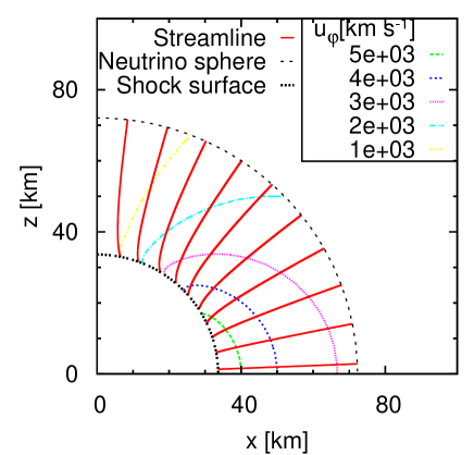
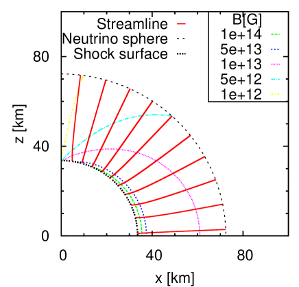
Figure 1: Streamlines in the meridian section (solid red lines) for the models rotation (left) and toroidal magnetic field (right). The mass accretion rate and neutrino luminosity are set to $\dot{M}=0.5~{}\mathrm{M_{\odot}~{}s^{-1}}$ and $L_{\nu}=26\times 10^{51}~{}\mathrm{erg~{}s^{-1}}$, respectively. The innermost black-dotted curve is the neutrino sphere and the outermost black-dashed curve indicates the shock surface in each panel. In the left panel the dash-dotted lines denote the profile of the rotational velocity $u_{\varphi}$; the rotational frequency is $f_{1000\mathrm{km}}=0.2~{}\mathrm{s^{-1}}$ and the value of $\epsilon$ for shock deformation is $\epsilon=2.0\times 10^{-3}$. In the right panel the dash-dotted lines show the profile of the toroidal magnetic field $B_{\varphi}$; the strength of the toroidal magnetic field at the outer boundary is $B_{1000\mathrm{km}}=2\times 10^{12}~{}\mathrm{G}$ and $\epsilon=1.8\times 10^{-3}$.

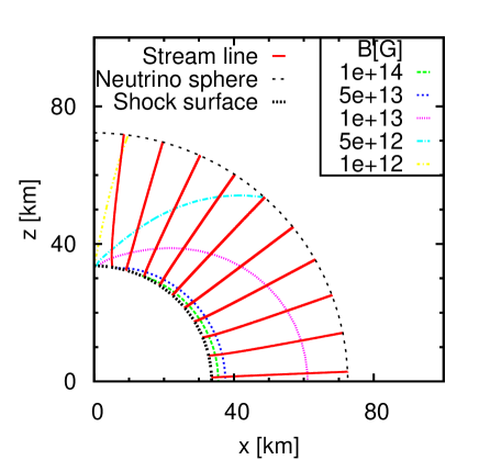
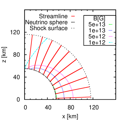
Figure 2: Same as in Figure 1 but for a model with different rotation and toroidal magnetic field (left) and for a model with poloidal magnetic field in addition (right). In the left panel the mass accretion rate and neutrino luminosity are set to $\dot{M}=0.5~{}\mathrm{M_{\odot}~{}s^{-1}}$ and $L_{\nu}=26\times 10^{51}~{}\mathrm{erg~{}s^{-1}}$, respectively. The rotational frequency is $f_{1000\mathrm{km}}=0.1~{}\mathrm{s^{-1}}$ and the strength of the toroidal magnetic field at the outer boundary is $B_{1000\mathrm{km}}=2\times 10^{12}~{}\mathrm{G}$. The value of $\epsilon$ for shock deformation is found to be $\epsilon=2.3\times 10^{-3}$. In the right panel the mass accretion rate and neutrino luminosity are set to $\dot{M}=2.0~{}\mathrm{M_{\odot}~{}s^{-1}}$ and $L_{\nu}=70\times 10^{51}~{}\mathrm{erg~{}s^{-1}}$. The rotational frequency is $f_{1000\mathrm{km}}=0.2~{}\mathrm{s^{-1}}$ and the strengths of the toroidal and poloidal magnetic fields are given as $B_{1000\mathrm{km}}=10^{12}~{}\mathrm{G}$ and $B_{0}=10^{11}~{}\mathrm{G}$ at the outer boundary. We find again that the value of $\epsilon$ for shock deformation is $\epsilon=2.3\times 10^{-3}$. The poloidal magnetic field lines are coincident with the streamlines because of the ideal MHD condition.

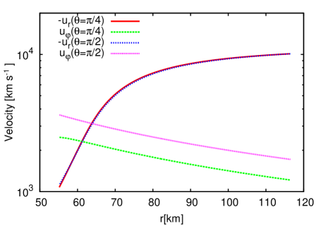
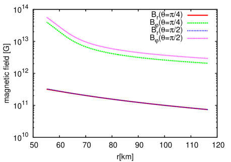
Figure 3: Radial profiles at $\theta=\pi/4$ and $\pi/2$ of the radial and azimuthal components of velocity (left) and magnetic field (right) of the model shown in the right panel of Figure 2. Both the poloidal and toroidal magnetic fields are taken into account.

Figure 1 displays streamlines in a meridian plane for a model either with rotation (left panel) or with toroidal magnetic field (right panel). In these models the neutrino luminosity and accretion rate are set as $L_{\nu}=26\times 10^{51}~{}\mathrm{erg}~{}\mathrm{s}^{-1}$ and $\dot{M}=0.5~{}\mathrm{M}_{\odot}\,\mathrm{s^{-1}}$. The innermost black-dotted curve indicates the neutrino sphere whereas the outermost black-dashed one corresponds to the stalled shock surface. We also draw the contour lines for the azimuthal components of velocity and magnetic field in the left and right panels, respectively. The values of $r_{s}$ and $\epsilon$ (see Equation 6) are $r_{s}\sim 70$ km and $\epsilon\sim 10^{-3}$ respectively, in both models. Interestingly, although the shapes of the shock surfaces are almost the same, being oblate, the flow pattern are different from each other. In fact in the left panel of Figure 1, the flow is pushed toward the equatorial plane as it approaches the PNS. This is due to centrifugal force and was previously seen in Figure 6 in Yamasaki & Yamada (2005). In the right panel, on the other hand, the flow is bent toward the symmetry axis. This is due to Lorentz force exerted by the toroidal magnetic field, which indeed behaves as a negative centrifugal force (e.g. Fujisawa 2015). Noted that the flow patterns of both models are similar near the rotation axis because of the boundary condition for $u_{\theta}$ at the axis (Equation 7).

The left panel in Figure 2 shows the result for a model with both rotation and toroidal magnetic field. The mass accretion rate, neutrino luminosity and strength of toroidal magnetic field are set to the same as values in Figure 1, but the rotation frequency is somewhat smaller. We find $\epsilon=2.3\times 10^{-3}$, slightly larger than in the previous cases in Figure 1. The centrifugal force and the Lorentz force almost cancel each other in this solution. The streamlines are nearly radial in this model except for the inner region where the Lorentz force is dominant over the centrifugal force and the streamlines look similar to those for purely toroidal magnetic field. This is understood from the conserved quantities $\ell$ and $\sigma$ along the streamline. As a matter of fact, $\ell$ does not depend on the density while $\sigma$ does as is clear in Equation (9). Since the density is low near the shock surface $\rho\sim 10^{9}~{}\mathrm{g~{}cm^{-3}}$ and gets higher toward the neutrino sphere, where $\rho\sim 10^{11}~{}\mathrm{g~{}cm^{-3}}$. The Lorentz force tends to be dominant in the inner region and vice versa.

The right panel in Figure 2 shows streamlines for a model that incorporates poloidal magnetic fields in addition to toroidal ones. The neutrino luminosity and accretion rate are set as $L_{\nu}=70\times 10^{51}~{}\mathrm{erg~{}s^{-1}}$ and $\dot{M}=2.0~{}\mathrm{M_{\odot}}~{}\mathrm{s}^{-1}$, respectively. The rotational frequency and the strength of magnetic fields are $f_{1000\mathrm{km}}=0.2~{}\mathrm{s^{-1}}$, $B_{1000\mathrm{km}}=10^{12}~{}\mathrm{G}$ and $B_{0}=10^{11}~{}\mathrm{G}$, respectively. Since the value of $B_{0}$ is smaller by an order than that of $B_{\mathrm{1000km}}$, the poloidal magnetic field in this model is much weaker than the toroidal magnetic field. We find that the value of $\epsilon$ is $\epsilon=2.3\times 10^{-3}$ again. Note that the poloidal magnetic field lines are aligned with the streamlines in ideal MHD. They are slightly curved near the neutrino sphere similarly to the left panel in Figure 1 because of Lorentz force mainly exerted by the toroidal magnetic field.

Figure 3 displays the radial and the azimuthal components of velocity (left) and magnetic field (right) at $\theta=\pi/4$ and $\theta=\pi/2$. The radial components of the flow velocities $u_{r}$ and of the poloidal magnetic field $B_{r}$ are almost identical at these zenith angles. This is mainly because of our assumption that the flow and the poloidal magnetic field outside the shock surface are radial and independent of $\theta$. If we had assumed a $\theta$-dependent functional form in Equation (15), for example, we would have found $\theta$-dependent radial profiles of $B_{r}$. In contrast, both $u_{\varphi}$ and $B_{\varphi}$ depend on $\theta$, being larger on equator ($\theta=\pi/2$) than at $\theta=\pi/4$. This $\theta$ dependence again ($\propto\sin\theta$), however, simply reflects of the functional forms for $u_{\varphi}$ and $B_{\varphi}$ in Equations (11) and (13).

The rotational velocity and toroidal magnetic field both increase inwards from the shock surface to the neutrino sphere. It is apparent, however, that the toroidal magnetic field rises more steeply than the rotational velocity. This trend is almost independent of the functional forms for $u_{\varphi}$ and $B_{\varphi}$. In fact, it is dictated by the conservation of $\ell$ and $\sigma$, the latter of which depends on the density profile as is explicit in Equation (B11) in Appendix B. One may hence roughly say that the $\theta$ dependence of the flow velocities and magnetic fields is mainly determined by their dependence just ahead of the shock wave, while their radial profiles are largely constrained by the conservation laws (Equation B11), being almost independent of the outer boundary conditions.

3.2 Effects of rotation and magnetic field on the critical luminosity

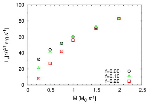
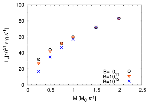
Figure 4: The critical luminosity as a function of the mass accretion rate for the models with rotation alone (left) and with purely toroidal magnetic field alone (right). The black circles represent the spherical models without rotation and magnetic field. In the left panel green triangle and red squares correspond to rotation rates $f_{1000\mathrm{km}}=0.1~{}\mathrm{s^{-1}}$ and $f_{1000\mathrm{km}}=0.2~{}\mathrm{s^{-1}}$, respectively. In the right panel field strength of $B_{1000\mathrm{km}}=10^{11}~{}\mathrm{G}$ and $B_{1000\mathrm{km}}=10^{12}~{}\mathrm{G}$, respectively.

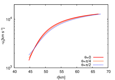
Figure 5: Radial profiles at $\theta=0$ (red solid lines), $\pi/4$ (red dotted lines) and $\pi/2$ (blue dotted lines) of the radial velocity for ones of the typical solutions at the critical neutrino luminosities for the models with rotation alone (left) and for the models with purely toroidal magnetic field alone (right panel). In the both panels the mass accretion rate and neutrino luminosity are set to $\dot{M}=2.0~{}\mathrm{M_{\odot}~{}s^{-1}}$ and $L_{\nu}=46\times 10^{51}~{}\mathrm{erg~{}s^{-1}}$, respectively. The rotational frequency is $f_{\mathrm{1000km}}=0.5~{}\mathrm{s^{-1}}$ (left) and the strength of the toroidal magnetic field is given as $B_{1000\mathrm{km}}=9\times 10^{12}~{}\mathrm{G}$ (right).

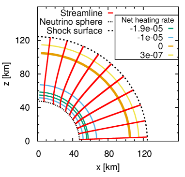
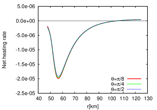
Figure 6: Streamlines (left) and net heating rates along some radial ray (right) in the meridian section for one of the purely rotational models at its critical luminosity. The mass accretion rate and neutrino luminosity are set to $\dot{M}=1.0~{}\mathrm{M_{\odot}~{}s^{-1}}$, $L_{\nu}=52\times 10^{51}~{}\mathrm{erg~{}s^{-1}}$, respectively. The rotational parameter is $f=0.2~{}\mathrm{s^{-1}}$ and the neutrino-heating rate is normalized by $c^{3}$. In the left panel the thick curve indicates the boundary between the heating region and the cooling region. In the right panel the three lines correspond to different zenith angles: $\theta=\pi/8$ (red solid line), $\theta=\pi/4$ (green dashed line) and $\theta=\pi/2$ (blue dotted line).

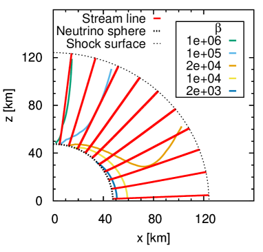
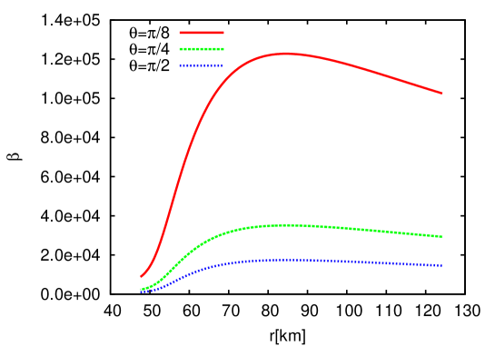
Figure 7: Streamlines (left) and radial profiles of plasma $\beta$ along some radial rays (right) for one of the purely toroidally-magnetized models close to its critical luminosity. The mass accretion rate and neutrino luminosity are set to $\dot{M}=1.0~{}\mathrm{M_{\odot}~{}s^{-1}}$, $L_{\nu}=52\times 10^{51}~{}\mathrm{erg~{}s^{-1}}$ and $B_{1000\mathrm{km}}=10^{12}~{}\mathrm{G}$, respectively. In the right panel the three lines correspond to different zenith angles: $\theta=\pi/8$ (red solid line), $\theta=\pi/4$ (green dashed line) and $\theta=\pi/8$ (blue dotted line).

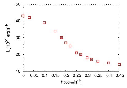
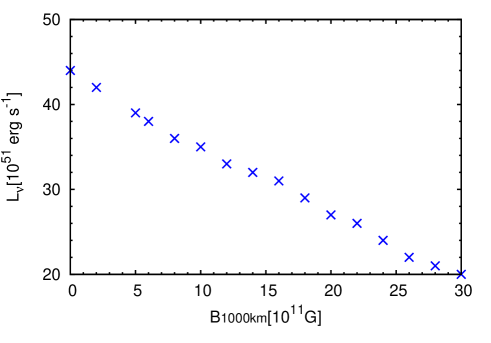
Figure 8: The critical luminosity as a function of the rotational rate $f_{1000\mathrm{km}}$ (left) and the strength of the toroidal magnetic field (right). The mass accretion rate is fixed to $\dot{M}=0.5\mathrm{M_{\odot}~{}s^{-1}}$.

Now we look into the changes in the critical luminosity that rotation and/or magnetic field produce. In this subsection we neglect poloidal magnetic fields ($B_{0}=0$) because the toroidal magnetic field is supposed to be dominant. Figure 4 displays the critical luminosities either for models with rotation alone (left panel) or for models with toroidal magnetic field alone with no rotation (right panel), which are plotted as a function of the mass accretion rate. As a reference, we also plot the critical luminosity of the spherical symmetric models without rotation and toroidal magnetic field as black circles.

It is evident among other things that the critical luminosity for all these models with either rotation or toroidal magnetic field are lower than those for the spherical models. Non-spherical forces, i.e., centrifugal forces and hoop stresses, tend to reduce the critical luminosity although the reduction rate depends on the mass accretion rate. As a matter of fact, for a given rotation velocity or magnetic field strength at the outer boundary, the critical luminosity gets lowered more strongly as the mass accretion rate becomes smaller: the reduction rate is as high as about $50\%$ – $70\%$ for the rapid rotation with $f_{\mathrm{1000km}}=0.2$ and $20\%$ – $50\%$ for the strong toroidal magnetic field with $B_{\mathrm{1000km}}=10^{12}~{}\mathrm{G}$ at the mass accretion rates lower than $1.0~{}\mathrm{M_{\odot}}$.

Figure 5 displays the radial profiles of the radial velocity $u_{r}$ along three radial rays with $\theta=0$ (red solid line), $\pi/4$ (orange dotted line) and $\pi/2$ (blue dashed line) for representative models on the critical curve either with a rotation alone (left panel) or with a toroidal magnetic field alone (right panel). The three profiles are almost the same at large radii in both panels whereas they are different from each other in the inner region. In the left panel for pure rotation, the radial infall velocity decreases more rapidly near the neutrino sphere along the rotation axis ($\theta=0$) than on the equator ($\theta=\pi/2$). This tendency was already observed in the previous work (Yamasaki & Yamada 2005). The radial profile of $u_{r}$ on the equator is convex at large radii but turns concave near the neutrino sphere whereas it remains convex along the polar axis as in the spherically symmetric case. Considering the fact that in the spherical symmetry the profile of the radial velocity is still convex near the inner boundary at the critical luminosity (see Figure 1 in Yamasaki & Yamada 2005), one may say that only the polar flow reaches the critical state locally and shock revival will commence there.

Interestingly, the situation is other way around in the right panel for the purely toroidal magnetic field. This is because such fields exert hoop stress, which behaves like a negative centrifugal force. As a result, the radial inflow velocity is smaller on the equator than on the axis near the neutrino sphere. According to the same argument, this may imply that only the equatorial flow becomes critical state locally and shock revival will be initiated on the equator. It is intriguing that the existence/non-existence of steady solutions that satisfy a certain boundary condition is itself a global issue while the critical state is realized locally as a result. Although some recent studies strongly deduce the presence of global conditions under critical state in spherical symmetry (e.g. Murphy & Dolence 2017), one may hence claim that the critical neutrino luminosity is determined both globally and locally.

Figure 6 displays the streamlines (left panel) and the radial profiles of the net heating rates along some radial rays (right panel) in the meridian section for one of the purely rotational models at its critical luminosity. The thick orange curve in the left panel indicates the boundary between the cooling and heating regions, or the 2D analog of the gain radius. One finds in the right panel that the cooling region near the pole (see the green line) is wider and deeper than that on the equator although the difference is not very large. Noted that for simplicity we assume in this paper that the neutrino sphere is spherical (see also Equation 4), which is certainly not true and tends to reduce the difference. We emphasize, however, that this slightly deformed cooling region results in the reduction of the critical neutrino luminosity as observed earlier.

Figure 7 shows distribution of the plasma $\beta$ defined as

$$\beta=\frac{8\pi p}{|B_{\varphi}|^{2}}.$$ (16)

in the meridian section for one of the non-rotating but purely toroidally-magnetized models close to its critical luminosity. The value of $\beta$ is very high, $>10^{3}$, almost everywhere in the computational domain, meaning that the magnetic pressure is much smaller than the matter pressure except near the equatorial area on the neutrino sphere where the value of $\beta$ is much smaller. This locally strong magnetic pressure (or locally low $\beta$) modifies the accretion flow there and gives rise to the critical state locally, leading to the reduction of the critical luminosity, as shown in the right panel of Figure 5.

Finally we show in Figure 8 the critical luminosity as a function of the rotational rate $f_{\mathrm{1000km}}$ (left) and the strength of the toroidal magnetic field $B_{\mathrm{1000km}}$ (right). We fix the mass accretion rate as $\dot{M}=0.5\mathrm{M_{\odot}}\,\mathrm{s^{-1}}$. The critical luminosities of solutions with $f_{1000\mathrm{km}}=0.25~{}\mathrm{s^{-1}}$ or $B_{\mathrm{1000km}}=3.0\times 10^{12}~{}\mathrm{G}$ are less than $20\times 10^{51}\mathrm{erg~{}s^{-1}}$. The critical luminosity is reduced by $\sim 70\%$ for the most rapid rotation and by $\sim 50\%$ for the strongest toroidal magnetic field, respectively. It is interesting that we cannot find a steady state solution for the rotation parameter $f_{1000\mathrm{km}}>0.45~{}\mathrm{s^{-1}}$ or the toroidal magnetic field strength $B_{1000\mathrm{km}}>3.0\times 10^{12}~{}\mathrm{G}$ because the shock surface comes too close to the neutrino sphere. These numerical results may imply that the existence of the critical specific angular momentum and the critical strength of the toroidal magnetic field, above which there actually exist no steady solutions.

4 Discussion and summary

We have derived numerically steady, non-spherical accretion flows through the standing shock wave onto the PNS solutions of stalled shock wave in the CCSNe core and effects of rotation and magnetic field on the shock revival in this paper. In order to obtain these steady solutions, we have developed a new numerical scheme to solve a system of nonlinear equations numerically, which we named the W4 method for non-linear equations, and we have indeed succeeded in generating various accretion flows with both rotation and magnetic field incorporated self-consistently in axisymmetric 2D. It should be noted that our new method can handle both poloidal and toroidal magnetic fields simultaneously.

Our main findings are summarized as follows.

1. The shock surface and the flow pattern become non-spherical by rotation and/or magnetic field in general. The shock surface is always oblate ($\epsilon>0$) whereas the stream lines are bent either toward the equatorial plane by rotation and poloidal magnetic field or toward the pole plane by toroidal magnetic field (Figures 1 and 2).

2. The toroidal magnetic field is dominant in the inner region (Figure 7) while the rotation is dominant in the outer region (Figures 2 and 3) because of the conserved quantities $\sigma$ and $\ell$ in Equations (9) and (B11).

3. The critical luminosity is lowered by rotation and/or magnetic field in general although the degree of reduction depends on the mass accretion rate (Figure 4).

4. In the presence of rotation and/or magnetic field the critical state is realized locally: either on the symmetry axis for rotation or on the equatorial plane for toroidal magnetic field (Figure 5) despite the solution itself is determined globally according to the boundary conditions.

5. The gain region in the accretion flow is also deformed. The cooling region is widened near the pole by the rotation (Figure 6) whereas it is affected mostly near the equator by the toroidal magnetic field (Figure 7). Although the deviation from the spherical symmetry is small, it results in the substantial reduction of the critical neutrino luminosity.

6. It is suggested the existence of the non-vanishing critical specific angular momentum, above which no steady solution exists irrespective of the neutrino luminosity (left panel in Figure 8). Our results are roughly consistent with the dynamical simulations in Iwakami et al. (2014a). We found that there also exists the critical strength of the toroidal magnetic field, above which no steady solution exists (right panel in Figure 8).

We ignore other non-spherical physical processes such as the turbulence in progenitors in this paper. Turbulence in the accretion flow enables explosion by changing the flow property. Murphy & Burrows (2008) performed 1D and 2D dynamical simulations and suggested that the reduction of critical luminosity is caused by turbulence. Murphy & Meakin (2011) examined many turbulent models using Reynolds decomposition and proposed a global turbulent model that reproduces the profiles and evolution of the simulations (see also 2D and 3D dynamical simulations by Murphy et al., 2013). Recently, Mabanta & Murphy (2018) considered 1D spherical steady models with the turbulence and contended that the turbulent dissipation rather than the ram pressure from the turbulence reduces the critical luminosity. The turbulent dissipation is a significant contributor to successful supernova explosion. Note that these works ignored the effect of magnetic fields. Masada et al. (2015), on the other hand, performed high resolution local simulations with magnetic field in a 3D thin layer to calculate the magneto-rotational-instability near the neutrino sphere accurately and found that the convectively stable layer around the neutrino sphere becomes fully turbulent due to the MRI. Magnetic field plays an important role on the turbulence.

The steady state problems concerning these physical processes, however, are considered in only 1D spherical models (e.g. Mabanta & Murphy 2018) and nobody has succeeded in obtaining the 2D steady accretion models with them. We will study the steady flows with them in 2D self-consistently using our numerical procedure and analyze the effect from them on the critical neutrino luminosity in the future.

Appendix A Rankine-Hugoniot relation on the deformed shock wave

\psfrag{er}{$\vec{e}_{r}$}\psfrag{vpa}{$\vec{u}_{\parallel}$}\psfrag{vpe}{$\vec{u}_{\perp}$}\psfrag{chi}{$\chi$}\psfrag{rs0}{$r=r_{sph}$}\psfrag{rs}{$r=r_{s}(\theta)$}\includegraphics[width=184.9429pt]{img/ShockShape2.eps}

\psfrag{x0}{$q=0$}\psfrag{x1}{$q=1$}\includegraphics[width=227.62204pt,clip]{img/surfacefitting.eps}

Figure 9: Schematic pictures of the oblique shock surface (left) and the surface-fitted coordinates (right). In the left picture the solid curve denotes the shock surface while dashed curve represents a sphere with the radius of $r=r_{\mathrm{sph.}}$. The angle between them is defined as $\chi$. In the right picture $q=0$ corresponds to the neutrino sphere surface whereas $q=1$ is the shock surface.

We need to impose the junction condition on the shock surface for each variable. We first define two unit vectors, $u_{\perp}$ and $u_{\parallel}$, each normal and tangential, respectively, to the shock surface given as $r=r_{s}(\theta)$. Then $\chi$ is defined to be the angle between the radial unit vector $e_{r}$ and $u_{\parallel}$ as shown in the left panel of Figure 9. The value of $\chi$ is obtained as follows:

$$\vec{u}_{\parallel}\cdot\vec{e}_{r}= |\vec{u}_{\parallel}|\cos\chi,$$ (A1a)

$$\cos\chi= \frac{{\rm d}r_{s}}{{\rm d}\theta}\left\{r_{s}^{2}+\left(\frac{{\rm d}r_{s}}{{\rm d}\theta}\right)^{2}\right\}^{-\frac{1}{2}}.$$ (A1b)

It is also useful to adopt the so-called surface-fitted coordinates $(q,\theta^{\prime})$ defined from the spherical coordinates ($r,\theta$) as

$$\displaystyle q\equiv\frac{r-r_{\nu}}{r_{s}(\theta)-r_{\nu}},$$ (A2)

$$\theta^{\prime}=\theta.$$ (A3)

This transformation maps the region between the neutrino sphere and the deformed shock surface into a domain given simply as

$$q\in[0,1],\ \theta^{\prime}\in[0,\pi].$$ (A4)

See the right panel of Figure 9. Noted that this is the domain of our main concern in this paper. The derivatives are also transformed as follows:

$$\frac{\partial Q}{\partial r}= \frac{1}{r_{s}-r_{\nu}}\frac{\partial Q}{\partial q},$$ (A5a)

$$\frac{\partial Q}{\partial\theta}= \frac{\partial Q}{\partial\theta^{\prime}}-\frac{q}{r_{s}-r_{\nu}}\frac{{\rm d}r_{s}}{{\rm d}\theta}\frac{\partial Q}{\partial q},$$ (A5b)

where $Q$ is a physical variable such as density or velocity. Henceforth, we will employ these surface-fitted coordinates alone and use the same notation $\theta$ instead of $\theta^{\prime}$ to denote the new angle coordinate.

The MHD Rankine-Hugoniot relation (e.g. Winterhalter et al. 1984; Takahashi & Yamada 2013) is written as follows:

$$\left[\rho\bm{u}\cdot\bm{n}\right]=0,$$ (A6a)

$$\left[\rho\left(\bm{u}\cdot\bm{n}\right)\bm{u}+\left(p+\frac{B^{2}}{8\pi}\right)\bm{n}-\frac{1}{4\pi}\left(\bm{B}\cdot\bm{n}\right)\bm{B}\right]=0,$$ (A6b)

$$\bigg{[}\bm{u}\cdot\bm{n}\left(\rho\varepsilon+p+\frac{1}{2}\rho u^{2}+\frac{B^{2}}{4\pi}\right)$$

$$-\frac{1}{4\pi}\left(\bm{B}\cdot\bm{n}\right)\left(\bm{B}\cdot\bm{u}\right)\bigg{]}=0,$$ (A6c)

$$\left[\bm{B}\cdot\bm{n}\right]=0,$$ (A6d)

$$\left[\bm{n}\times\left(\bm{u}\times\bm{B}\right)\right]=0,$$ (A6e)

where the background denotes as usual the difference between the upstream and downstream values of the quantity given inside the bracket and we use the ordinary notation $\bm{n}$ for the normal vector to the shock surface. One can also express these relations as

$$\rho u_{\perp}=\hat{\rho}\hat{u}_{\perp},$$ (A7a)

$$\rho u_{\perp}\bm{u}+\left(p+\frac{B^{2}}{8\pi}\right)\bm{n}-\frac{1}{4\pi}B_{\perp}\bm{B}$$

$$=\hat{\rho}\hat{u}_{\perp}\hat{\bm{u}}+\left(\hat{p}+\frac{\hat{B}^{2}}{8\pi}\right)\bm{n}-\frac{1}{4\pi}\hat{B}_{\perp}\hat{\bm{B}},$$ (A7b)

$$u_{\perp}\left(\rho\epsilon+p+\frac{1}{2}\rho u^{2}+\frac{B^{2}}{4\pi}\right)-\frac{1}{4\pi}B_{\perp}\left(\bm{B}\cdot\bm{u}\right)$$

$$=\hat{u}_{\perp}\left(\hat{\rho}\hat{\epsilon}+\hat{p}+\frac{1}{2}\hat{\rho}\hat{u}^{2}+\frac{\hat{B}^{2}}{4\pi}\right)-\frac{1}{4\pi}\hat{B}_{\perp}\left(\hat{\bm{B}}\cdot\hat{\bm{u}}\right),$$ (A7c)

$$B_{\perp}=\hat{B}_{\perp},$$ (A7d)

$$B_{\perp}\bm{u}-u_{\perp}\bm{B}=\hat{B}_{\perp}\hat{\bm{u}}-\hat{u}_{\perp}\hat{\bm{B}},$$ (A7e)

where the hat $\,\hat{}\,$ means the upstream value and the subscript _⟂ denotes the normal component to the shock surface. We use these relations to obtain the downstream values of physical quantities. The rotation and magnetic field upstream the shock are given in Section 2.3 (see also Appendix B).

Since we have assumed a free-falling cold, spherical flow outside the shock surface, the radial velocity $u_{f}$, density $\rho_{f}$ and pressure $p_{f}$ just ahead of the shock surface are given as follows:

$$u_{f}(r)= -\sqrt{\frac{2GM}{r}},$$ (A8a)

$$\rho_{f}(r)= -\frac{\dot{M}}{4\pi r^{2}u_{f}}=\frac{\dot{M}}{\sqrt{32\pi^{2}GM}}r^{-\frac{3}{2}},$$ (A8b)

$$p_{f}(r)= 0.$$ (A8c)

Note that the mass accretion rate is positive ($\dot{M}>0$) in this paper.

Appendix B The rotation law and magnetic-field profile outside the shock wave

Here we explain in detail the ideas behind the setting of the outer boundary conditions for rotation and magnetic field. If the magnetic field is purely toroidal ($B_{r}=B_{\theta}=0$), there are two conserved quantities: specific angular momentum $\ell$ and a quantity related with the magnetic torque $\sigma$. The former comes from the $\varphi$ component of the Euler equation (Equation 1) and the latter results from the $\varphi$ component of the ideal MHD condition. They are constant along each streamline. It should be noted that the specific entropy is not conserved, since heating and cooling are taken into account in our formulation unlike the previous works that assumed the barotropic (adiabatic) condition (e.g. Lovelace et al. 1986; Fujisawa et al. 2013). The conservations of $\ell$ and $\sigma$ are expressed as

$$\ell(\psi)=r\sin\theta u_{\varphi},$$ (B1a)

$$\sigma(\psi)=\frac{B_{\varphi}}{r\sin\theta\rho},$$ (B1b)

where $\ell(\psi)$ and $\sigma(\psi)$ are arbitrary functions of $\psi$, which is a so-called stream function defined in the following relations:

$$u_{r}\equiv\frac{1}{4\pi\rho r^{2}\sin\theta}\frac{\partial\psi}{\partial\theta},\ u_{\theta}\equiv-\frac{1}{4\pi\rho r\sin\theta}\frac{\partial\psi}{\partial r}.$$ (B2)

Since we have assumed that the flow is spherical outside the shock surface, the stream function there is given explicitly as

$$\psi=\dot{M}\cos\theta.$$ (B3)

We need to specify the functional forms of $\ell$ and $\sigma$ to fix the rotation law and the profile of toroidal magnetic field. In this paper following Yamasaki & Yamada (2005) we specify the angular distributions of $u_{\varphi}$ and $B_{\varphi}$ at $r=1000~{}\mathrm{km}$. Since the stream function depends only on $\theta$ alone (see Equation B3), $\ell$ and $\sigma$ are also the functions of $\theta$ alone and the $u_{\varphi}$ and $B_{\varphi}$ at $r=1000~{}\mathrm{km}~{}(\equiv r_{\mathrm{1000km}})$ are expressed as follows:

$$u_{\varphi}(r_{1000\mathrm{km}},\theta) =\frac{\ell(\theta)}{r_{1000\mathrm{km}}\sin\theta},$$ (B4a)

$$B_{\varphi}(r_{1000\mathrm{km}},\theta) =r_{1000\mathrm{km}}\sin\theta\rho_{1000\mathrm{km}}\sigma(\theta)$$

$$=\frac{\dot{M}}{\sqrt{32\pi^{2}GMr_{1000\mathrm{km}}}}\sin\theta\sigma(\theta),$$ (B4b)

where $\rho_{1000\mathrm{km}}$ is the density at $r_{\mathrm{1000km}}$. Just as in Yamasaki & Yamada (2005) we assume uniform rotation at $r_{\mathrm{1000km}}$ with a rotational frequency $f_{1000\mathrm{km}}$. The $\ell(\theta)$ is given as

$$\ell(\theta)=2\pi r^{2}_{1000\mathrm{km}}f_{1000\mathrm{km}}\sin^{2}\theta.$$ (B5)

The azimuthal component of velocity is also obtained as follows:

$$u_{\varphi}(r,\theta)=2\pi\frac{r_{1000\mathrm{km}}^{2}}{r}\sin\theta f_{1000\mathrm{km}}.$$ (B6)

As for $\sigma$, we simply assume that it is independent of $\theta$ at $r_{\mathrm{1000km}}$:

$$\sigma(\theta)=-\frac{\sqrt{32\pi^{2}GM}}{\dot{M}}B_{1000\mathrm{km}}\sqrt{r_{1000\mathrm{km}}}.$$ (B7)

Then the profile of the toroidal magnetic field is given as follows:

$$B_{\varphi}(r,\theta)=B_{1000\mathrm{km}}\sqrt{\frac{r_{1000\mathrm{km}}}{r}}\sin\theta,$$ (B8)

where the $B_{1000\mathrm{km}}$ is the strength of toroidal magnetic field at $r_{\mathrm{1000km}}$. Note that the profiles of $u_{\varphi}$ and $B_{\varphi}$ thus obtained apparently satisfy the boundary conditions on the symmetry axis and the equator in Equation (7).

Next we consider the case, in which the magnetic field has both poloidal and toroidal components. Then the situation is more complicated with $\ell$ and $\sigma$ being no longer independent of each other (Fujisawa et al. 2013). From the continuity equation of magnetic field ($\nabla\cdot\bm{B}=0$), the magnetic flux function $\Psi$ is defined to give the poloidal magnetic-field components as

$$B_{r}=\frac{1}{r^{2}\sin\theta}\frac{\partial\Psi}{\partial\theta},\,\,\,\,B_{\theta}=-\frac{1}{r\sin\theta}\frac{\partial\Psi}{\partial r}.$$ (B9)

Since the poloidal magnetic-field lines are coincide with the streamlines in ideal MHD, the magnetic flux function is also constant along each streamline,

$$\Psi\equiv\Psi(\psi).$$ (B10)

Then $\ell$ and $\sigma$ are expressed in terms of the magnetic flux function, which is in turn a function of the stream function alone (see Fujisawa et al. 2013) as

$$\ell(\psi) =r\sin\theta u_{\varphi}-r\sin\theta\frac{d\Psi(\psi)}{d\psi}B_{\varphi},$$ (B11a)

$$\sigma(\psi) =\frac{B_{\varphi}}{r\sin\theta\rho}-\frac{4\pi}{r\sin\theta}u_{\varphi}\frac{d\Psi(\psi)}{d\psi}.$$ (B11b)

Note that the specific angular momentum ($r\sin\theta u_{\varphi}$) is no longer conserved along a streamline but the $\ell$ is sill and $\sigma$ too remains a conserved quantity although it also contains a term that depends on $\Psi$.

Just as in the previous case, in which the purely toroidal magnetic field is considered, we set the functional form of $\Psi$ outside the shock surface from the condition that the streamlines and hence the poloidal magnetic-field line are spherical as follows:

$$\Psi =-r_{\mathrm{1000km}}^{2}B_{0}\cos\theta,$$ (B12a)

$$B_{r}(r,\theta) =\frac{r^{2}_{\mathrm{1000km}}}{r^{2}}B_{0},$$ (B12b)

$$\frac{d\Psi}{d\psi} =-r_{\mathrm{1000km}}^{2}\frac{B_{0}}{\dot{M}}={\mathrm{constant}},$$ (B12c)

where $B_{0}$ is a constant corresponding to the strength of poloidal magnetic field at $r_{\mathrm{1000km}}$. It is apparent from Equation (B12b) that the radial magnetic field does not depend on $\theta$ outside the shock surface. Since the $\theta$ component of magnetic field vanishes $B_{\theta}=0$ outside the shock surface, the $\varphi$ component of the ideal MHD condition given in Equation (2) becomes

$$\frac{\partial}{\partial r}\left(rB_{r}u_{\varphi}-rB_{\varphi}u_{r}\right)=0$$ (B13a)

$$\Rightarrow\left(rB_{r}u_{\varphi}-rB_{\varphi}u_{r}\right)=C_{1}(\theta),$$ (B13b)

$$\Rightarrow\frac{u_{\varphi}}{r\sin\theta}\frac{d\Psi}{d\psi}\frac{\partial\psi}{\partial\theta}-\frac{B_{\varphi}}{4\pi\rho r\sin\theta}\frac{\partial\psi}{\partial\theta}=C_{1}(\theta).$$ (B13c)

In the above equations, $C_{1}$ is a function of $\theta$ alone and is related with $\sigma$ as follows (see Equation B11b):

$$\sigma(\theta)=-4\pi\left(\frac{\partial\psi}{\partial\theta}\right)^{-1}C_{1}(\theta).$$ (B14)

The $\varphi$ component of the equations of motion (Equation 1) can be recast in a similar way as

$$u_{r}\frac{\partial u_{\varphi}}{\partial r}+u_{r}\frac{u_{\varphi}}{r}-\frac{B_{r}}{4\pi\rho}\left(\frac{\partial B_{\varphi}}{\partial r}+\frac{B_{\varphi}}{r}\right)=0$$ (B15a)

$$\Rightarrow\frac{\partial}{\partial r}(ru_{\varphi})-\frac{B_{r}}{4\pi\rho u_{r}}\frac{\partial}{\partial r}\left(rB_{\varphi}\right)=0$$ (B15b)

$$\Rightarrow ru_{\varphi}-\frac{B_{r}}{4\pi\rho u_{r}}\left(rB_{\varphi}\right)=C_{2}(\theta),$$ (B15c)

$$\Rightarrow ru_{\varphi}-r\frac{d\Psi}{d\psi}B_{\varphi}=C_{2}(\theta),$$ (B15d)

where we use the fact that $B_{r}/(\rho u_{r})$ is constant in the current case. $C_{2}$ is again related with $\ell$ (see Equation B11a) as

$$\ell(\theta)=\sin\theta C_{2}(\theta).$$ (B16)

Using $C_{1}$ and $C_{2}$ instead of $\ell$ and $\sigma$, we express $B_{\varphi}$ and $u_{\varphi}$ as

$$B_{\varphi} =\left(r\frac{u_{r}}{B_{r}}-\frac{r^{3}B_{r}}{\dot{M}}\right)^{-1}\left(C_{2}-\frac{C_{1}}{B_{r}}\right),$$ (B17a)

$$u_{\varphi} =\left(r-\frac{r^{3}B_{r}^{2}}{\dot{M}u_{r}}\right)^{-1}\left(C_{2}-\frac{r^{2}B_{r}}{u_{r}\dot{M}}C_{1}\right).$$ (B17b)

It is apparent from these expressions that there may exist a singularity on a surface, where the radial velocity becomes equal to the Alfvén velocity $u_{A}^{2}=B_{r}^{2}/(4\pi\rho)$. In this paper, we do not deal with this problem but simply avoid it by choosing the value of $B_{0}$ so that no such singular surface would not be encountered.

In actual computations, we set the values of $f_{\mathrm{1000km}}$ and $B_{\mathrm{1000km}}$ and obtain those of $u_{\varphi}$ and $B_{\varphi}$ at $r_{\mathrm{1000km}}$ as

$$u_{\varphi}(r_{\mathrm{1000km}},\theta) =2\pi r_{1000\mathrm{km}}\sin\theta f_{1000\mathrm{km}},$$ (B18a)

$$B_{\varphi}(r_{\mathrm{1000km}},\theta) =B_{1000\mathrm{km}}\sin\theta,$$ (B18b)

and then we derive the values of $u_{\varphi}(r_{s},\theta)$ and $B_{\varphi}(r_{s},\theta)$ just ahead of the shock wave by solving Equations (B13a) and (B15a) numerically.

Appendix C Numerical procedure

Here we outline the procedure to solve the non-linear differential equations that describe the steady, shocked, non-spherical accretion flows. The system of equations given in Section 2 is formally written as

$$\mathcal{A}\left(\bm{Q}\right)\frac{\partial\bm{Q}}{\partial q}+\mathcal{B}\left(\bm{Q}\right)\frac{\partial\bm{Q}}{\partial\theta}+\mathcal{C}\left(\bm{Q}\right)=0,$$ (C1)

where we introduce the variable vector $\bm{Q}\equiv\left[\rho\ u_{r}\ u_{\theta}\ u_{\varphi}\ T\ B_{r}\ B_{\theta}\ B_{\varphi}\right]^{T}$ for brevity; $\mathcal{A}\left(\bm{Q}\right),\mathcal{B}\left(\bm{Q}\right)$ and $\mathcal{C}\left(\bm{Q}\right)$ are matrix-valued nonlinear function of $\bm{Q}$. Note that the shock surface corresponds to $q=1$ on the surface-fitted coordinates. Equations (C1) are discretized at the cell-center in the $q$-mesh while at the grid point in the $\theta$-mesh as follows:

$$\bm{F}_{j-1,k}\equiv\mathcal{A}\left(\bm{Q}_{j-\frac{1}{2},k}\right)\frac{\bm{Q}_{j,k}-\bm{Q}_{j-1,k}}{q_{j}-q_{j-1}}+\mathcal{B}\left(\bm{Q}_{j-\frac{1}{2},k}\right)\frac{\bm{Q}_{j-\frac{1}{2},k+1}-\bm{Q}_{j-\frac{1}{2},k-1}}{2\Delta\theta}+\mathcal{C}\left(\bm{Q}_{j-\frac{1}{2},k}\right)=0,$$ (C2)

where $\bm{Q}_{j-\frac{1}{2},k}$ is defined as

$$\bm{Q}_{j-\frac{1}{2},k}=\frac{1}{2}\left(\bm{Q}_{j-1,k}+\bm{Q}_{j,k}\right).$$ (C3)

The set of algebraic nonlinear Equations (C2) is solved numerically with the W4 method in Appendix D.

We take the following steps to obtain a solution:

1. We first fix the five model parameters $\dot{M}$, $L_{\nu}$, $f_{1000\mathrm{km}}$, $B_{1000\mathrm{km}}$ and $B_{0}$. Then the inner boundary $r_{\nu}$ is determined from Equation (5). We give an initial guess to the shape of shock surface $r_{s}(\theta)$, which determines the angle $\chi$ in Equation (A1b).

2. The density, velocity and pressure outside the shock are given in Equation (A8) and other variables such as $u_{\varphi}$, $B_{\varphi}$ and $B_{r}$ are determined as explained in Appendix B.

3. Given the upstream quantities, the corresponding downstream quantities are obtained as mentioned by solving the Rankine-Hugoniot relation given in Equation (A7). In particular, the radial and $\theta$ components of the velocity and magnetic field just behind the shock front are given in terms of the parallel ($u_{\parallel},B_{\parallel}$) and perpendicular ($u_{\perp},B_{\perp}$) components of velocity and magnetic field as

   $$u_{r}= u_{\parallel}\cos\chi+u_{\perp}\sin\chi,$$ (C4a)

   $$u_{\theta}= u_{\parallel}\sin\chi-u_{\perp}\cos\chi,$$ (C4b)

   $$B_{r}= B_{\parallel}\cos\chi+B_{\perp}\sin\chi,$$ (C4c)

   $$B_{\theta}= B_{\parallel}\sin\chi-B_{\perp}\cos\chi.$$ (C4d)

4. We integrate the basic equations (Equations 1 and  2) inward from the outer boundary $q=1$ to the inner boundary $q=0$. If the density $\rho$ obtained at the inner boundary differs from the specified value $\rho=10^{11}~{}\mathrm{g~{}cm^{-3}}$, we modify the shock surface, changing $r_{\mathrm{sph}}$ and/or $\epsilon$ and repeat the iteration steps 3 and 4 until the correct value of $\rho$ is obtained at the inner boundary.

We change the value of neutrino luminosity $L_{\nu}$ and repeat the above procedures until we obtain a series of solutions up to the critical point.

Appendix D Details of the W4 method

The Newton-Raphson method is one of the simplest and the most commonly used methods to solve systems of nonlinear equations numerically. It is very efficient, converging to a root quadratically, if it really converges, which happens normally when the initial guess is sufficiently close to the root (Press et al. 1992). The W4 method of our own devising is an iterative relaxation method just like the Newton-Raphson method and some of its extensions, quasi-Newton method (e.g. Broyden’s method, Broyden 1965). Unlike these Newton-type methods, the W4 method uses acceleration and damping terms in addition to the velocity term for convergence. In fact, thanks to these terms, the W4 method shows better global convergence: we obtain the solutions that Newton-type cannot. We explain the W4 method in detail, staring with a brief of introducing its new extension.

D.1 Newton-Raphson method

In this paper we solve a system of nonlinear equations numerically to obtain steady accretion flows through a standing shock wave onto a PNS. Such a problem can be written generically as

$$F_{i}(x_{1},x_{2},\cdots,x_{N})=0\hskip 10.0pti=1,2,\cdots,N,$$ (D1)

for $N$ variables $x_{i},i=1,2,\cdots,N$. For notational convenience we let $\bm{x}$ and $\bm{F}$. In solving this type of equations, the Newton-Raphson method is probably the first choice. In the Newton-Raphson method, each function $F_{i}$ is Taylor-expanded to the first order at a certain $x$ (Press et al. 1992) as

$$F_{i}(\bm{x}+\delta\bm{x})=F_{i}(\bm{x})+\sum_{j=1}^{N}\frac{\partial F_{i}}{\partial x_{j}}\delta x_{j}+{\cal O}(\delta\bm{x}^{2}).$$ (D2)

The Jacobian matrix is then introduced

$$J_{ij}\equiv\frac{\partial F_{i}}{\partial x_{j}}.$$ (D3)

We solve the linearized equations

$$F_{i}(\bm{x}+\delta\bm{x})=F_{i}(\bm{x})+\sum_{j=1}^{N}J_{ij}\delta x_{j}=0,$$ (D4)

for $\delta x_{j}$ as

$$\delta x_{i}=-\sum_{j=1}^{N}J^{-1}_{ij}F_{j},$$ (D5)

where $J^{-1}_{ij}$ is the inverse of the Jacobian matrix. The value of $x$ is then incremented by $\delta x$ and Equation (D1) is solved for this new $x$. The procedure is repeated until the sequence $x_{n}$ determined from

$$\bm{x}^{n+1}=\bm{x}^{n}+\delta\bm{x},$$ (D6)

is converged. Whereas in the Newton-Raphson method the correction terms $\delta\bm{x}$ is calculated with the inverse of the Jacobian matrix as in Equation (D5), it is obtained in different ways (e.g. good and bad Broyden’s method, Broyden 1965) in the secant methods or other Newton-type methods. Regardless, it is important that all these methods employ Equation (D6) for a single step evolution. We modify this in the W4 method.

D.2 W4 method

Equation (D6), which is used for the single-step evolution commonly in the Newton-type methods, may be recast in to the following suggestive form: If we introduce a time step width $d\tau$, Equation (D6) becomes as

$$\frac{\bm{x}^{n+1}-\bm{x}^{n}}{\Delta\tau}=\bm{f}(\bm{x}),\hskip 10.0pt\bm{f}(\bm{x})\equiv\frac{\delta\bm{x}}{\Delta\tau}=-\frac{\mathbf{J}^{-1}\bm{F}}{\Delta\tau}.$$ (D7)

where $\Delta\tau$ is a fictitious time step, which is arbitrary for the moment.

Then the resultant equation may be interpreted as an approximation to the following first-order differential equations:

$$\frac{d\bm{x}}{d\tau}=\bm{f}(\bm{x}).$$ (D8)

It is probably not surprising then to consider differential equations of second order instead of first order given as follows:

$$\frac{d^{2}\bm{x}}{d\tau^{2}}+\mathbf{M}_{1}\frac{d\bm{x}}{d\tau}+\mathbf{M}_{2}\bm{F}=0,$$ (D9)

where $\mathbf{M}_{1}$ and $\mathbf{M}_{2}$ are matrices somehow related with the Jacobian matrix. Note that these equations remind us of the forced oscillation of connected springs with damping. This analogy is important and useful in considering the behaviour of solutions. Introducing ”momentum” $\bm{p}$, we can decompose these second order differential equations into two sets of first order differential equations as follows:

$$\frac{d\bm{x}}{d\tau}=\mathbf{X}\bm{p},\hskip 10.0pt\frac{d\bm{p}}{d\tau}=-2\bm{p}-\mathbf{Y}\bm{F},$$ (D10)

where $\mathbf{X}$ and $\mathbf{Y}$ are matrices related with $\bm{F}$ and the Jacobian matrix. Finite-differencing these first-order differential equations, we obtain a new recurrence formula for the single-step evolution as

$$\bm{x}^{n+1}=\bm{x}^{n}+\Delta\tau\mathbf{X}\bm{p}^{n},\hskip 10.0pt\bm{p}^{n+1}=(1-2\Delta\tau)\bm{p}^{n}-\Delta\tau\mathbf{Y}\bm{F}.$$ (D11)

These are the single-step evolution equations adopted in the W4 method. It should be apparent that this is an extension of Equation (D6). It should be emphasized, however, that there is a greater degree of freedom in choosing $\mathbf{X}$ and $\mathbf{Y}$. Indeed we have studied various choices and found that UL decomposition of the Jacobian matrix show a nice performance in finding roots. In this decomposition $\mathbf{J}\equiv\mathbf{U}\mathbf{L}$, $\mathbf{U}$ and $\mathbf{L}$ are upper and lower triangular matrices given, respectively, as follows:

$$\mathbf{U}=\left(\begin{array}[]{cccc}u_{11}&u_{12}&u_{13}\\ 0&u_{22}&u_{23}\\ 0&0&u_{33}\\ \end{array}\right),\hskip 10.0pt\mathbf{L}=\left(\begin{array}[]{cccc}1&0&0\\ \ell_{21}&1&0\\ \ell_{31}&\ell_{32}&1\\ \end{array}\right),$$ (D18)

where $u_{ij}$ and $\ell_{ij}$ are elements of these matrices for the case of a $3\times 3$ matrix. Setting $\mathbf{X}=\mathbf{L}^{-1}$ and $\mathbf{Y}=\mathbf{D}^{-1}$ as well as $\Delta\tau=0.5$, we obtain in the version we refer to as the UL-W4 method (Okawa et al. 2018)

$$\bm{x}^{n+1}=\bm{x}^{n}+\frac{1}{2}\mathbf{L}^{-1}_{n}\bm{p}^{n},\hskip 10.0pt\bm{p}^{n+1}=-\frac{1}{2}\mathbf{U}^{-1}_{n}\bm{F}(\bm{x}^{n}),\hskip 10.0pt$$ (D19)

where $\mathbf{L}_{n}^{-1}$ and $\mathbf{U}_{n}^{-1}$ denote $\mathbf{L}^{-1}$ and $\mathbf{U}^{-1}$ at $n$-th time step, respectively. Note that combined Equations (D19)

$$\bm{x}^{n+1}=\bm{x}^{n}-\frac{1}{4}\mathbf{L}^{-1}_{n}\mathbf{U}^{-1}_{n-1}\bm{F}(\bm{x}^{n-1}),$$ (D20)

differ from the single-step evolution equation in the Newton-Raphson method because $\mathbf{L}^{-1}_{n}\mathbf{U}^{-1}_{n-1}\neq\mathbf{J}^{-1}_{n}$ and $\mathbf{L}^{-1}_{n}\mathbf{U}^{-1}_{n-1}\neq\mathbf{J}^{-1}_{n-1}$ in general. It should be also stressed that the product tends to the inverse of the Jacobian matrix $\mathbf{L}^{-1}_{n}\mathbf{U}^{-1}_{n-1}\simeq\mathbf{J}^{-1}_{n-1}\simeq\mathbf{J}^{-1}_{n}$ as the sequence approaches the root. These properties turn out to be crucial for both global and local convergences (Okawa et al. 2018).

Another useful choice of $\mathbf{X}$ and $\mathbf{Y}$ is derived from the LH decomposition of the Jacobian matrix, which is in turn based on QR decomposition of the transposed Jacobian matrix $(\mathbf{J}^{T}\equiv\mathbf{Q}\mathbf{R})$, where $\mathbf{H}$ is a Householder matrix, $\mathbf{Q}$ is an orthogonal matrix and $\mathbf{R}$ is an upper triangular matrix. Let us describe the procedure of these decompositions for a $3\times 3$ Jacobian matrix, which is expressed as

$$\mathbf{J}^{T}=\mathbf{A}_{(0)}\equiv\left(\begin{array}[]{ccc}a_{11}^{(0)}&a_{12}^{(0)}&a_{13}^{(0)}\\ a_{21}^{(0)}&a_{22}^{(0)}&a_{23}^{(0)}\\ a_{31}^{(0)}&a_{32}^{(0)}&a_{33}^{(0)}\end{array}\right).$$ (D24)

First, we extract the first column of this matrix as a column vector $\bm{a}_{(0)}\equiv\left[a_{11}^{(0)}\ a_{21}^{(0)}\ a_{31}^{(0)}\right]^{T}$, and make another vector $\bm{b}_{(0)}$ with the norm $|\bm{a}_{(0)}|$ as

$$\bm{b}_{(0)}\equiv\left[-{\rm sign}\left(a_{11}^{(0)}\right)|\bm{a}_{(0)}|\ 0\ 0\right]^{T},$$ (D25)

where we use the sign function. The Householder matrix $\mathbf{H}_{(0)}\equiv\mathbf{E}-2\bm{c}_{(0)}\bm{c}_{(0)}^{T}$, where $\mathbf{E}$ denotes the identity matrix,

$$\bm{c}_{(0)}\equiv\frac{\bm{a}_{(0)}-\bm{b}_{(0)}}{|\bm{a}_{(0)}-\bm{b}_{(0)}|},$$ (D26)

and transforms the vector $\bm{a}_{(0)}$ into $\bm{b}_{(0)}$ or vice versa: $\mathbf{H}_{(0)}\bm{a}_{(0)}=\bm{b}_{(0)}$ and $\mathbf{H}_{(0)}\bm{b}_{(0)}=\bm{a}_{(0)}$. Multiplying this Householder matrix with $\mathbf{A}_{(0)}$, we obtain

$$\mathbf{H}_{(0)}\mathbf{A}_{(0)}\equiv\mathbf{A}_{(1)}=\left(\begin{array}[]{ccc}r_{11}&r_{12}&r_{13}\\ 0&a_{22}^{(1)}&a_{23}^{(1)}\\ 0&a_{32}^{(1)}&a_{33}^{(1)}\end{array}\right),$$ (D30)

where $r_{1j}$ and $a_{ij}^{(1)}$ are the components of the matrix $\mathbf{A}_{(1)}$ thus obtained, which are non-vanishing in general.

We repeat the same process to the lower right $2\times 2$ submatrix. We again extract the column vector $\bm{a}_{(1)}\equiv\left[a_{22}^{(1)}\ a_{32}^{(1)}\right]^{T}$ and make a new vector $\bm{b}_{(1)}\equiv\left[-{\rm sign}\left(a_{22}^{(1)}\right)|\bm{a}_{(1)}|\ 0\right]^{T}$ and construct another Householder matrix

$$\mathbf{H}_{(1)}\equiv\left(\begin{array}[]{cc}1&\bm{0}\\ \bm{0}&\quad\mathbf{E}-2\bm{c}_{(1)}\bm{c}_{(1)}^{T}\end{array}\right),$$ (D33)

where $\mathbf{E}$ and $\bm{c}_{(1)}\equiv(\bm{a}_{(1)}-\bm{b}_{(1)})/|\bm{a}_{(1)}-\bm{b}_{(1)}|$ are now $2\times 2$ matrices. We multiply it with $\mathbf{A}_{(1)}$ and obtain the following:

$$\mathbf{H}_{(1)}\mathbf{A}_{(1)}\equiv\mathbf{A}_{(2)}=\mathbf{H}_{(1)}\mathbf{H}_{(0)}\mathbf{J}^{T}=\left(\begin{array}[]{ccc}r_{11}&r_{12}&r_{13}\\ 0&r_{22}&r_{23}\\ 0&0&r_{33}\end{array}\right)=\mathbf{R}.$$ (D37)

It is clear from these equations that the product of the two Householder matrices make the transposed Jacobian matrix to the upper triangular matrix $\mathbf{R}$. Since the Householder matrix $\mathbf{H}$ is orthogonal and symmetric ($\mathbf{H}^{T}=\mathbf{H}^{-1}=\mathbf{H}$) by construction, the Jacobian matrix is decomposed as follows:

$$\mathbf{J}^{T}=\mathbf{H}_{(0)}\mathbf{H}_{(1)}\mathbf{R}\ \Rightarrow\ \mathbf{J}=(\mathbf{H}_{(0)}\mathbf{H}_{(1)}\mathbf{R})^{T}=\mathbf{L}\mathbf{H}_{(1)}\mathbf{H}_{(0)},$$ (D38)

where $\mathbf{L}$ is the transpose of $\mathbf{R}$ and a lower triangular matrix.

Finally, we set $\mathbf{X}$ and $\mathbf{Y}$ as $\mathbf{X}=\mathbf{H}_{(1)}\mathbf{L}^{-1}$ and $\mathbf{Y}=\mathbf{H}_{(0)}$. Then, Equations (D11) become

$$\bm{x}^{n+1}=\bm{x}+\frac{1}{2}\mathbf{H}_{(0)}\bm{p}^{n},\hskip 10.0pt\bm{p}^{n+1}=-\frac{1}{2}\mathbf{H}_{(1)}\mathbf{L}^{-1}\bm{F}(\bm{x}).\hskip 10.0pt$$ (D39)

Although we explain the procedure for the $3\times 3$ Jacobian matrix, the generalization to other dimensions should be obvious: if the dimension is larger than 4, we set $\mathbf{X}=\mathbf{H}_{(0)}$ and $\mathbf{Y}=\cdots\mathbf{H}_{(3)}\mathbf{H}_{(2)}\mathbf{H}_{(1)}\mathbf{L}^{-1}$.

We have applied the W4 method to various problems and found more often not that it can find a root even initial guesses are not close to the root and other Newton-type methods such as the original Newton-Raphson method and Broyden method fail to reach it. This is also the case for the problem of our interest in this paper, that is, solving the (M)HD equations numerically to obtain the steady accretion flows through a stalled shock wave onto the PNS. These facts indicate that the W4 method of our own devising has a better global convergence property than those other methods. We stress that the UL or LH decomposition introduced above are just two useful possibilities and the W4 method has much greater possibilities. We refer readers to Okawa et al. (2018) for more mathematical aspects of the method and numerical tests.

Appendix E Convergence test

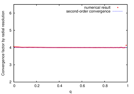
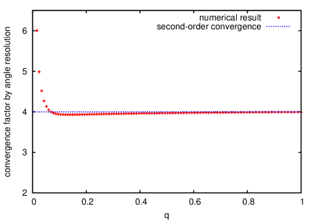
Figure 10: Convergence factors $Q_{q}$ (left) and $Q_{\theta}$ (right) as functions of the $q$ with $N_{q}=200$ and $N_{\theta}=20$. The mass accretion rate and neutrino luminosity are set to $\dot{M}=\mathrm{2.0~{}M_{\odot}~{}s^{-1}}$ and $L_{\nu}=4.5\times 10^{52}~{}\mathrm{ergs~{}s^{-1}}$, respectively. The rotational frequency is $f_{\mathrm{1000km}}=0.03~{}\mathrm{s^{-1}}$ and the strengths of the toroidal and poloidal magnetic fields are given as $B_{\mathrm{0}}=10^{6}~{}\mathrm{G}$ and $B_{\mathrm{1000km}}=10^{6}~{}\mathrm{G}$ at the outer boundary. The dotted blue line denotes the second-order convergence ($Q=4$).

We check the convergence of the numerical solutions we obtain in this paper by changing the number of grid points. We use the results with three different numbers of grid points and check the convergence factors $Q_{q}$ and $Q_{\theta}$ (e.g. Okawa et al. 2014) as follows:

$$Q_{q}\equiv\left|\frac{\phi_{2N_{q}}-\phi_{N_{q}}}{\phi_{N_{q}}-\phi_{N_{q}/2}}\right|,$$ (E1a)

$$Q_{\theta}\equiv\left|\frac{\phi_{2N_{\theta}}-\phi_{N_{\theta}}}{\phi_{N_{\theta}}-\phi_{N_{\theta}/2}}\right|,$$ (E1b)

where $N_{q}$ and $N_{\theta}$ denote the numbers of grid in the $q$-direction and $\theta$-direction and $\phi_{N_{q}}$ and $\phi_{N_{\theta}}$ are physical quantities calculated with $N_{r}$-grids and $N_{\theta}$-grids. We here use the $\theta$-averaged tangential component of velocity

$$\phi(q)=\frac{1}{N_{\theta}}\sum_{k=1}^{N_{\theta}}u_{\theta}(q,\theta_{k}),$$ (E2)

because it is easily influenced by the numerical errors at boundaries. Since we use the cell-centered second-order discretization in both directions as in Equations (C2 and C3), the convergence factors must be $Q\sim 4$ if the numerical results are converged well. In the convergence test the mass accretion rate and neutrino luminosity are set to $\dot{M}=\mathrm{2.0~{}M_{\odot}~{}s^{-1}}$ and $L_{\nu}=4.5\times 10^{52}~{}\mathrm{ergs~{}s^{-1}}$, respectively. The rotational frequency is $f_{\mathrm{1000km}}=0.03~{}\mathrm{s^{-1}}$ and the strengths of the toroidal and poloidal magnetic fields are given as $B_{\mathrm{0}}=10^{6}~{}\mathrm{G}$ and $B_{\mathrm{1000km}}=10^{6}~{}\mathrm{G}$ at the outer boundary.

Figure 10 displays the convergence factor $Q_{q}$ (left) and $Q_{\theta}$ (right) as functions of $q$ with $N_{q}=200$ and $N_{\theta}=20$. It is obvious that our code actually has the second-order convergence with respect to both $N_{q}$ and $N_{\theta}$ with these grid numbers. Note that the solutions are almost unchanged with $N_{\theta}\sim 20$, especially near the neutrino sphere. The actual number $N_{q}$, on the other hand, depends on the mass accretion rate $\dot{M}$ and the numerical scheme employed but the typical value is $N_{q}\sim 100$ for high mass accretion rates and $N_{q}\sim 1000$ for models with low mass accretion rates. The LH-W4 method requires smaller values of $N_{q}$ than the UL-W4 method. We hence set $N_{\theta}\sim 20$ and $N_{q}\sim 100$ for models with high mass accretion rates and $N_{q}\sim 1000$ for models with low mass accretion rates for the numerical computations in this paper.

References

- Akiyama et al. (2003) Akiyama, S., Wheeler, J. C., Meier, D. L., & Lichtenstadt, I. 2003, ApJ, 584, 954
- Blondin & Mezzacappa (2007) Blondin, J. M., & Mezzacappa, A. 2007, Nature, 445, 58
- Blondin et al. (2003) Blondin, J. M., Mezzacappa, A., & DeMarino, C. 2003, ApJ, 584, 971
- Broyden (1965) Broyden, C. 1965, Mathematics of Computation, 19, 577
- Bruenn et al. (2009) Bruenn, S. W., Mezzacappa, A., Hix, W. R., et al. 2009, in Journal of Physics Conference Series, Vol. 180, Journal of Physics Conference Series, 012018
- Bruenn et al. (2016) Bruenn, S. W., Lentz, E. J., Hix, W. R., et al. 2016, ApJ, 818, 123
- Burrows (2013) Burrows, A. 2013, Reviews of Modern Physics, 85, 245
- Burrows et al. (2007) Burrows, A., Dessart, L., Livne, E., Ott, C. D., & Murphy, J. 2007, ApJ, 664, 416
- Burrows & Goshy (1993) Burrows, A., & Goshy, J. 1993, ApJ, 416, L75
- Burrows et al. (2006) Burrows, A., Livne, E., Dessart, L., Ott, C. D., & Murphy, J. 2006, ApJ, 640, 878
- Burrows et al. (2018) Burrows, A., Vartanyan, D., Dolence, J. C., Skinner, M. A., & Radice, D. 2018, Space Sci. Rev., 214, 33
- Couch (2013) Couch, S. M. 2013, ApJ, 775, 35
- Couch et al. (2015) Couch, S. M., Chatzopoulos, E., Arnett, W. D., & Timmes, F. X. 2015, ApJ, 808, L21
- Couch & Ott (2013) Couch, S. M., & Ott, C. D. 2013, ApJ, 778, L7
- Couch & Ott (2015) —. 2015, ApJ, 799, 5
- Dimmelmeier et al. (2002) Dimmelmeier, H., Font, J. A., & Müller, E. 2002, A&A, 388, 917
- Dolence et al. (2015) Dolence, J. C., Burrows, A., & Zhang, W. 2015, ApJ, 800, 10
- Fernández (2015) Fernández, R. 2015, MNRAS, 452, 2071
- Fernández et al. (2014) Fernández, R., Müller, B., Foglizzo, T., & Janka, H.-T. 2014, MNRAS, 440, 2763
- Foglizzo et al. (2015) Foglizzo, T., Kazeroni, R., Guilet, J., et al. 2015, PASA, 32, e009
- Fryer & Heger (2000) Fryer, C. L., & Heger, A. 2000, ApJ, 541, 1033
- Fujisawa (2015) Fujisawa, K. 2015, MNRAS, 450, 4016
- Fujisawa et al. (2013) Fujisawa, K., Takahashi, R., Yoshida, S., & Eriguchi, Y. 2013, MNRAS, 431, 1453
- Gabay et al. (2015) Gabay, D., Balberg, S., & Keshet, U. 2015, ApJ, 815, 37
- Guilet et al. (2010) Guilet, J., Sato, J., & Foglizzo, T. 2010, ApJ, 713, 1350
- Hanke et al. (2013) Hanke, F., Müller, B., Wongwathanarat, A., Marek, A., & Janka, H.-T. 2013, ApJ, 770, 66
- Heger et al. (2005) Heger, A., Woosley, S. E., & Spruit, H. C. 2005, ApJ, 626, 350
- Herant et al. (1992) Herant, M., Benz, W., & Colgate, S. 1992, ApJ, 395, 642
- Hunter et al. (2008) Hunter, I., Lennon, D. J., Dufton, P. L., et al. 2008, A&A, 479, 541
- Iwakami et al. (2008) Iwakami, W., Kotake, K., Ohnishi, N., Yamada, S., & Sawada, K. 2008, ApJ, 678, 1207
- Iwakami et al. (2014a) Iwakami, W., Nagakura, H., & Yamada, S. 2014a, ApJ, 793, 5
- Iwakami et al. (2014b) —. 2014b, ApJ, 786, 118
- Janka et al. (2012) Janka, H.-T., Hanke, F., Hüdepohl, L., et al. 2012, Progress of Theoretical and Experimental Physics, 2012, 01A309
- Janka & Mueller (1996) Janka, H.-T., & Mueller, E. 1996, A&A, 306, 167
- Keshet & Balberg (2012) Keshet, U., & Balberg, S. 2012, Physical Review Letters, 108, 251101
- Kotake et al. (2004) Kotake, K., Sawai, H., Yamada, S., & Sato, K. 2004, ApJ, 608, 391
- Kotake et al. (2012) Kotake, K., Sumiyoshi, K., Yamada, S., et al. 2012, Progress of Theoretical and Experimental Physics, 2012, 01A301
- Kotake et al. (2003) Kotake, K., Yamada, S., & Sato, K. 2003, ApJ, 595, 304
- Kuroda et al. (2012) Kuroda, T., Kotake, K., & Takiwaki, T. 2012, ApJ, 755, 11
- Kuroda et al. (2016) Kuroda, T., Takiwaki, T., & Kotake, K. 2016, ApJS, 222, 20
- Lentz et al. (2015) Lentz, E. J., Bruenn, S. W., Hix, W. R., et al. 2015, ApJ, 807, L31
- Liebendörfer et al. (2001) Liebendörfer, M., Mezzacappa, A., Thielemann, F.-K., et al. 2001, Phys. Rev. D, 63, 103004
- Liebendörfer et al. (2005) Liebendörfer, M., Rampp, M., Janka, H.-T., & Mezzacappa, A. 2005, ApJ, 620, 840
- Lovelace et al. (1986) Lovelace, R. V. E., Mehanian, C., Mobarry, C. M., & Sulkanen, M. E. 1986, ApJS, 62, 1
- Mabanta & Murphy (2018) Mabanta, Q. A., & Murphy, J. W. 2018, ApJ, 856, 22
- Marek & Janka (2009) Marek, A., & Janka, H.-T. 2009, ApJ, 694, 664
- Masada et al. (2015) Masada, Y., Takiwaki, T., & Kotake, K. 2015, ApJ, 798, L22
- Melson et al. (2015) Melson, T., Janka, H.-T., & Marek, A. 2015, ApJ, 801, L24
- Mösta et al. (2015) Mösta, P., Ott, C. D., Radice, D., et al. 2015, Nature, 528, 376
- Müller (2016) Müller, B. 2016, PASA, 33, e048
- Müller et al. (2012) Müller, B., Janka, H.-T., & Marek, A. 2012, ApJ, 756, 84
- Murphy & Burrows (2008) Murphy, J. W., & Burrows, A. 2008, ApJ, 688, 1159
- Murphy & Dolence (2017) Murphy, J. W., & Dolence, J. C. 2017, ApJ, 834, 183
- Murphy et al. (2013) Murphy, J. W., Dolence, J. C., & Burrows, A. 2013, ApJ, 771, 52
- Murphy & Meakin (2011) Murphy, J. W., & Meakin, C. 2011, ApJ, 742, 74
- Nagakura et al. (2017) Nagakura, H., Iwakami, W., Furusawa, S., et al. 2017, ApJS, 229, 42
- Nagakura et al. (2014) Nagakura, H., Sumiyoshi, K., & Yamada, S. 2014, ApJS, 214, 16
- Nagakura et al. (2013) Nagakura, H., Yamamoto, Y., & Yamada, S. 2013, ApJ, 765, 123
- Nagakura et al. (2018) Nagakura, H., Iwakami, W., Furusawa, S., et al. 2018, ApJ, 854, 136
- Nakamura et al. (2014) Nakamura, K., Kuroda, T., Takiwaki, T., & Kotake, K. 2014, ApJ, 793, 45
- Nakamura et al. (2015) Nakamura, K., Takiwaki, T., Kuroda, T., & Kotake, K. 2015, PASJ, 67, 107
- Nordhaus et al. (2010) Nordhaus, J., Burrows, A., Almgren, A., & Bell, J. 2010, ApJ, 720, 694
- Obergaulinger et al. (2006) Obergaulinger, M., Aloy, M. A., & Müller, E. 2006, A&A, 450, 1107
- Obergaulinger et al. (2014) Obergaulinger, M., Janka, H.-T., & Aloy, M. A. 2014, MNRAS, 445, 3169
- Obergaulinger et al. (2018) Obergaulinger, M., Just, O., & Aloy, M. A. 2018, Journal of Physics G Nuclear Physics, 45, 084001
- O’Connor & Couch (2018) O’Connor, E. P., & Couch, S. M. 2018, ApJ, 854, 63
- Ohnishi et al. (2006) Ohnishi, N., Kotake, K., & Yamada, S. 2006, ApJ, 641, 1018
- Okawa et al. (2014) Okawa, H., Cardoso, V., & Pani, P. 2014, Phys. Rev. D, 90, 104032
- Okawa et al. (2018) Okawa, H., Fujisawa, K., Yamamoto, Y., et al. 2018, arXiv
- Ott et al. (2012) Ott, C. D., Abdikamalov, E., O’Connor, E., et al. 2012, Phys. Rev. D, 86, 024026
- Pan et al. (2016) Pan, K.-C., Liebendörfer, M., Hempel, M., & Thielemann, F.-K. 2016, ApJ, 817, 72
- Pejcha & Thompson (2012) Pejcha, O., & Thompson, T. A. 2012, ApJ, 746, 106
- Potter et al. (2012) Potter, A. T., Chitre, S. M., & Tout, C. A. 2012, MNRAS, 424, 2358
- Press et al. (1992) Press, W. H., Teukolsky, S. A., Vetterling, W. T., & Flannery, B. P. 1992, Numerical recipes in FORTRAN. The art of scientific computing
- Raives et al. (2018) Raives, M. J., Couch, S. M., Greco, J. P., Pejcha, O., & Thompson, T. A. 2018, ArXiv e-prints, arXiv:1801.02626
- Ramírez-Agudelo et al. (2013) Ramírez-Agudelo, O. H., Simón-Díaz, S., Sana, H., et al. 2013, A&A, 560, A29
- Rampp & Janka (2002) Rampp, M., & Janka, H.-T. 2002, A&A, 396, 361
- Roberts et al. (2016) Roberts, L. F., Ott, C. D., Haas, R., et al. 2016, ApJ, 831, 98
- Sawai et al. (2005) Sawai, H., Kotake, K., & Yamada, S. 2005, ApJ, 631, 446
- Sawai & Yamada (2014) Sawai, H., & Yamada, S. 2014, ApJ, 784, L10
- Sawai & Yamada (2016) —. 2016, ApJ, 817, 153
- Scheck et al. (2006) Scheck, L., Kifonidis, K., Janka, H.-T., & Müller, E. 2006, A&A, 457, 963
- Shibata & Sekiguchi (2004) Shibata, M., & Sekiguchi, Y.-I. 2004, Phys. Rev. D, 69, 084024
- Shibata & Sekiguchi (2005) —. 2005, Phys. Rev. D, 71, 024014
- Sumiyoshi et al. (2005) Sumiyoshi, K., Yamada, S., Suzuki, H., et al. 2005, ApJ, 629, 922
- Summa et al. (2018) Summa, A., Janka, H.-T., Melson, T., & Marek, A. 2018, ApJ, 852, 28
- Suwa et al. (2010) Suwa, Y., Kotake, K., Takiwaki, T., et al. 2010, PASJ, 62, L49
- Suwa et al. (2016) Suwa, Y., Yamada, S., Takiwaki, T., & Kotake, K. 2016, ApJ, 816, 43
- Takahashi et al. (2016) Takahashi, K., Iwakami, W., Yamamoto, Y., & Yamada, S. 2016, ApJ, 831, 75
- Takahashi & Yamada (2013) Takahashi, K., & Yamada, S. 2013, Journal of Plasma Physics, 79, 335
- Takahashi & Yamada (2014) —. 2014, ApJ, 794, 162
- Takiwaki et al. (2009) Takiwaki, T., Kotake, K., & Sato, K. 2009, ApJ, 691, 1360
- Takiwaki et al. (2012) Takiwaki, T., Kotake, K., & Suwa, Y. 2012, ApJ, 749, 98
- Takiwaki et al. (2014) —. 2014, ApJ, 786, 83
- Takiwaki et al. (2016) —. 2016, MNRAS, 461, L112
- Thompson et al. (2005) Thompson, T. A., Quataert, E., & Burrows, A. 2005, ApJ, 620, 861
- Wade & MiMeS Collaboration (2015) Wade, G. A., & MiMeS Collaboration. 2015, in Astronomical Society of the Pacific Conference Series, Vol. 494, Physics and Evolution of Magnetic and Related Stars, ed. Y. Y. Balega, I. I. Romanyuk, & D. O. Kudryavtsev, 30
- Wilson (1985) Wilson, J. R. 1985, in Numerical Astrophysics, ed. J. M. Centrella, J. M. Leblanc, & R. L. Bowers, 422
- Winterhalter et al. (1984) Winterhalter, D., Kivelson, M. G., Walker, R. J., & Russell, C. T. 1984, Advances in Space Research, 4, 287
- Wongwathanarat et al. (2010) Wongwathanarat, A., Janka, H.-T., & Müller, E. 2010, ApJ, 725, L106
- Yamada & Sawai (2004) Yamada, S., & Sawai, H. 2004, ApJ, 608, 907
- Yamasaki & Yamada (2005) Yamasaki, T., & Yamada, S. 2005, ApJ, 623, 1000
- Yamasaki & Yamada (2007) —. 2007, ApJ, 656, 1019