Divide-and-Conquer Strategy for Large-Scale Eulerian Solvent Excluded Surface

Abstract

Motivation: Surface generation and visualization are some of the most important tasks in biomolecular modeling and computation. Eulerian solvent excluded surface (ESES) software provides analytical solvent excluded surface (SES) in the Cartesian grid, which is necessary for simulating many biomolecular electrostatic and ion channel models. However, large biomolecules and/or fine grid resolutions give rise to excessively large memory requirements in ESES construction. We introduce an out-of-core and parallel algorithm to improve the ESES software.
Results: The present approach drastically improves the spatial and temporal efficiency of ESES. The memory footprint and time complexity are analyzed and empirically verified through extensive tests with a large collection of biomolecule examples. Our results show that our algorithm can successfully reduce memory footprint through a straightforward divide-and-conquer strategy to perform the calculation of arbitrarily large proteins on a typical commodity personal computer. On multi-core computers or clusters, our algorithm can reduce the execution time by parallelizing most of the calculation as disjoint subproblems. Various comparisons with the state-of-the-art Cartesian grid based SES calculation were done to validate the present method and show the improved efficiency. This approach makes ESES a robust software for the construction of analytical solvent excluded surfaces.
Availability and implementation: http://weilab.math.msu.edu/ESES.

1 Introduction

As a principal tool to study the biomolecular world, molecular modeling and analysis have an increasing impact in computational biology. The accuracy and efficiency of molecular modeling and analysis are often crucial in enabling more sophisticated downstream research. Researchers have made persistent efforts in reconstructing and visualizing the details of biomolecules through various simplifications, including the ball-and-stick model by von Hofmann, dated back to 1865, and the ribbon diagram by Richardson for illustrating protein structures. However, in order to simulate physical phenomena like the electrostatic distribution of macromolecules in a cellular environment, a much more elaborate model is needed to describe the interface between solvent and solute regions. The van der Waals surface (i.e., “atom and bond” model by Corey and Pauling in 1953) was introduced to describe such interfaces, where each type of atoms was described by a sphere with the corresponding van der Waals radius. For various simulations and geometric smoothness, concepts of solvent accessible surface (SAS) [7, 18] and solvent excluded surface (SES) [12, 17] were built on top of the van der Waals radii. SAS captures the trajectory of the center of a probe atom rolling on the van der Waals surface as the interface delineating the boundary of regions accessible by the center of any solvent molecule. SES is defined by the boundary of the union of all possible outside probe balls, and thus consists of three types of patches. Specifically, convex patches, where the probe touches one of the atoms of the molecule, saddle patches, where the probe touches two atoms, and concave patches, where the probe touches three or more atoms, are parts of an SES for a biomolecule.

All of these models still fail to guarantee the interface smoothness, as singularities and sharp edges cannot be completely avoided for the aforementioned geometry models for biomolecules. Minimal molecular surface (MMS) based on the mean curvature flow was introduced to resolve this issue [3, 2]. Various Gaussian surfaces [4, 9, 25, 23, 5, 8], skinning surface [6] and flexibility-rigidity index (FRI) surface [22, 16] have been proposed to achieve a similar goal. Another limitation for these models is that they only reflect the static or instantaneous shape in vacuum. In practice, solvent and solute interactions, making a static interface inaccurate for certain biophysical analysis. Thus, various solvent-solute interactive boundaries were proposed [10, 21]. However, despite its weaknesses, SES remains the most favorable model among biophysicists, due to its simplicity and effectiveness in capturing the interface of solvent and solute through its definition, with which various physical phenomena can be described with a reasonable accuracy.

Many software packages were developed to calculate SES [19]. Among them, MSMS is of considerable influence [20]. Built on top of MSMS, there are various software packages for different purposes. For the Lagrangian representation, a triangle mesh can be directly constructed for the three different types of patches followed by a concatenation. Nevertheless, MSMS is known for its efficiency and robustness issues, which often occur when large protein molecules and fine resolutions are required [14]. Moreover, many biophysical phenomena are happening not only on the surface, but inside the encapsulated volume of the molecules. To address these issues and meet the requirements of volumetric output, Liu et al. [14] introduced an Eulerian solvent excluded surface (ESES) approach as an alternative for surfaces represented as intersections and normals with a regular Cartesian grid. The ESES algorithm starts with a list of atoms describing the molecule enclosed by a regular Cartesian grid. Based on the three different types of patches for SES, all grid points are classified as either inside or outside with respect to SES. Finally, intersection points are computed on each mesh line with two ends on opposite side of the interface. It is also straightforward to be converted into the Lagrangian representation, i.e., a triangle mesh, through the marching cubes algorithm. Although high accuracy and robustness are well addressed with this method, it often suffers from the lack of efficiency as well as overly large memory requirements, as a full regular grid has to be maintained. The ESES algorithm is sequential, which results in long execution time especially when the grid resolution increases due to a fine grid spacing or large protein complexes with many atoms [13].

In this work, we propose an out-of-core parallelizable version of ESES, in which we divide the bounding box of the molecule into tiled sub-blocks based on the localized nature of the problem. By performing the computation based on local information, one can avoid keeping the whole grid and all the atoms in memory, and at the same time, distribute the computation to multiple processors. Thus, for large molecules or fine grids, both space and time efficiency can be substantially improved. By restricting the active subdomains that are being executed, the whole procedure can always be done on a personal computer (PC) with a fixed memory, e.g., 2GB. Testing and comparison are done on the 2016 core set of PDBbind database (http://www.pdbbind.org.cn/), with additional validation by users worldwide through the authors’ website for the project.

The rest of the paper is organized as follows. Section 2 discusses design of the improved algorithm with locality. Section 3 is devoted to the space and time complexity analysis of the proposed algorithm. The validation and comparison of our results are carried out in Section 4. Section 5 concludes the paper with a comment on future work.

2 Algorithm

2.1 Recap of ESES

As we aim at improving the efficiency of ESES [14], we assume the same input, a list $\mathcal{A}$ of atoms, represented by the center location $\bm{c}_{i}$ and the corresponding van der Waals radius $r_{i}$ for each atom,

$$\mathcal{A}=\{(\bm{c}_{i},r_{i})\}_{i=1\dots N},$$ (1)

where $N$ is the number of atoms.

We also assume the same output: first, a 3D array of Boolean indicating whether each grid point is inside the molecule surface,

$$\rm{Inside}\left[i,j,k\right]=\left\{\begin{array}[]{ll}1,&\hbox{$(ih,jh,kh)\in M$}\\ 0,&\hbox{otherwise,}\end{array}\right.$$ (2)

where $h$ is the grid spacing, and $M$ is the volume enclosed by SES; and second, a set of intersection points between grid edges and the SES

$$\mathcal{I}=\{\bm{s},\bm{t},\lambda_{st}\}_{\bm{st}\in\mathcal{E}},$$ (3)

where $\bm{s}$ and $\bm{t}$ are grid points with $\bm{st}$ representing the corresponding edge, and $\mathcal{E}$ is the grid edge set with two grid points adjacent to each other and ${\rm{Inside}}[\bm{s}]\neq{\rm{Inside}}[\bm{t}]$. The location of the intersection point can be computed through

$$\bm{p}=\lambda_{st}\bm{s}+(1-\lambda_{st})\bm{t}.$$ (4)

Note that, using the connectivity construction procedure in the standard marching cubes algorithm, we can also output a triangle mesh based on the Eulerian output.

2.2 Overview

The main idea for reducing the main memory requirement is through a simple domain decomposition without the need to explicitly handle the boundary matching problem. Owing to the locality of the ESES algorithm, we can straightforwardly decompose the computational domain into many non-overlapping subdomains. With each subdomain retaining only a small number of atoms that are less than the largest van der Waals radius away from the subdomain boundary, we have all the information necessary to determine the inside and the outside information, as well as the intersections of the SES surface and the grid edges within the subdomain. Thus, we can successfully reduce the memory footprint by controlling the size of each subdomain so as to fit within the main memory limit of a typical PC. The memory storage for the list of atoms relevant for the subdomain is negligible compared to the storage requirement for the subgrid, since the grid spacing in practical applications would typically be smaller than the van der Waals radius of the smallest atom.

As shown in Figure 1, patches rendered with different color belong to different subdomains, and they can be independently constructed by intersection detection locally within the corresponding subdomain, followed by using the marching cubes algorithm. With a direct concatenation of all the output, we can construct the whole molecular surface. It is also possible for the downstream applications to choose only the subdomains relevant for the calculation that they perform.

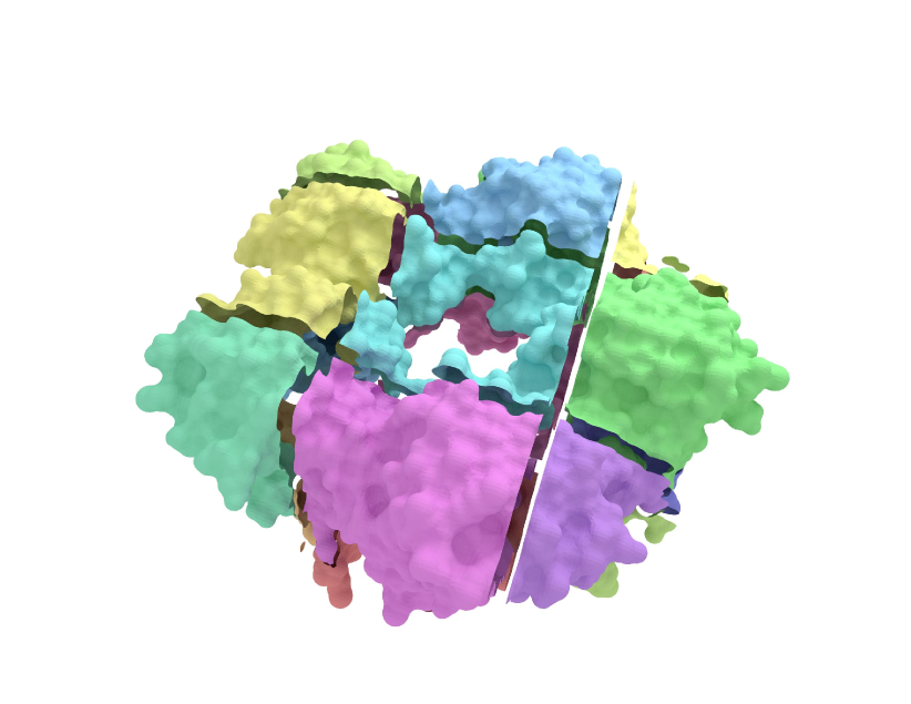
Figure 1: Illustration of subdomain based algorithm. The bounding box of the whole molecular surface is divided into several non-overlapping subdomains, which can be computed independently with a small memory footprint. Finally, patches of the SES from each subdomain can be assembled into a watertight surface identical to the one constructed with ESES. Note that the patches form a watertight surface, the gaps between the adjacent patches from different subdomains are added for visualization only.

When designing a parallelizable out-of-core algorithm, the first and foremost problem to deal with is to analyze the dependence among different steps of the procedure or different parts of the data. In this section, we examine the four main stages of the ESES algorithm [14]:

• construction of the grid and the analytical expression for patches of the SES,

• classification of the grid points to the inside points or the outside points of the SES,

• calculation of the intersection between grid edges and the SES,

• and assembly of the output.

When performed in a subdomain of the entire domain, the first three steps need to performed in the given order, but they do not have data dependence to the calculation done on any other subdomain. For instance, the classification of any grid point can be locally determined by the nearby atoms, more precisely, atoms at a distance less than the sum of the probe radius and the largest van der Waals radius. Similarly, where the intersection is on a grid edge depends only on the SES analytical patch expressions determined by nearby atoms. Thus we can set up one thread per subdomain, without any possibility of race conditions, i.e., our output is independent on the timing of each thread.

If file I/O exchanges are done through sequential devices such as a hard drive, the final output step would have to be done after finishing the previous three steps. On the other hand, if the final output is to reside in a random access memory, once the size of output for each subdomain is determined, it is possible to assemble the output in sublinear time. If the file system allows for concatenation without moving data blocks, it is also possible for each thread to write to a different file, and concatenate them in a time linear manner with respect to the number of subdomains.

As in ESES, for the robustness of the calculation, there are some grid points left undetermined as inside or outside in the second step, and only finalized in the third step after the intersections of nearby grid edges are determined [14]. Nevertheless, this procedure will only have a local data dependence. Thus, partitioning the whole grid into several subdomains does not change the final classification of such points. As confirmed by our large set of test results, the uncertain grids are rare as indicated by [14], and when they indeed exist, their classification in the subdomain based approach is identical to that in the original ESES.

In sum, we can safely assume that there is no communication of information between intermediate results from different subdomains. This implies that we can do out-of-core calculation by loading only one subdomain, and/or parallelizing the calculation by simultaneously initiating one thread per subdomain.

2.3 Decomposition to subdomains

The entire calculation domain in ESES is a regular Cartesian grid inside a cuboid. Typically, it is constructed as a tight bounding box of the list of the atoms, padded with a few additional layers of grid cells to provide some margin for easy handling of the boundary cells.

Therefore, it is a natural choice to design the subdomain as non-overlapping cubes with the same number of grid cells in each of the three dimensions. The domain can be extended slightly if the size of the original entire domain in any direction is not a multiple of the size of the subdomain. We will call a cubic subdomain as a block, following the similar term used in CUDA parallel thread mapping design.

By focusing on the local computation within each block, the memory footprint is mainly determined by the size of the block, since we only need to keep one block in the main memory at a time. Some memory storage is required to store the list of atoms relevant for the analytical SES patch construction. If we store the entire list of atoms, for large molecules, it can still require a large block of memory, and may require more time to perform the nearest neighbor search. Fortunately, due to the localized nature of the calculation, it is possible to determine whether an atom is inside or within a small distance from a block. The rest of the atoms do not need to reside in the memory, and one can treat the calculation inside the block as if it were for a smaller molecule, without any unfavorable effect on the final output.

2.4 Index mapping

After the computation is done for each individual block, we need to map the result within that block to the original domain. The index mapping is similar to the CUDA parallel thread mapping design for 3D. We illustrate the basic idea in 2D through Figure 2. Each block has coordinates $(b_{x},b_{y},b_{z})$ indicating the position of its top left back corner. Assuming that the grid cell count along one edge of each block is $(b_{s})$, for a grid point with local coordinates $(i,j,k)$ in the block, its corresponding global coordinates are found through the following function

$$\mathrm{LocalToGlobal}(i,j,k;b_{x},b_{y},b_{z})=(b_{s}b_{x}+i,b_{s}b_{y}+j,b_{s}b_{z}+k).$$ (5)

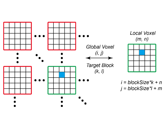
Figure 2: 2D Index mapping Example. All the indices are 0-based. Given a cell with global coordinates $(i,j)$ in block $(k,l)$ (green) and its local coordinates $(m,n)$ within the block, the one-to-one mapping is straightforward as illustrated. Note that $(m,n)$ would require fewer bits to store than $(i,j)$. This is typical in parallel processing such as CUDA threads.

2.5 Subdomain boundary treatment

While the subdomains are not overlapping with the outer boundary of the total computational domain, they may intersect at a zero-measure set, such as a common rectangle, a common line segment, or a common point. Thus, during the final assembly of the output from all the blocks, the boundary grid points and boundary grid edges are to be carefully handled. Otherwise, redundant information for grid point classification and intersection points on subdomain boundaries may appear in the output. For instance, whether a grid point is inside may be duplicated up to 8 times, if it is at the corner point shared by 8 subdomains. Similarly, the intersection information may also be duplicated up to 4 times, if a grid edge is shared by 4 subdomains.

One way to eliminate the redundancy is to add a post-processing step. However, using ideas commonly used for eliminating such redundancies, we can directly avoid the generation of redundant data. This more efficient approach is based on the partitioning of the domain into truly disjoint subdomains, each of which has the form of a half-open half-closed box, in other words, the Cartesian product of three half-open half-closed intervals:

$$[b_{s}b_{x},b_{s}b_{x}+b_{s})\times[b_{s}b_{y},b_{s}b_{y}+b_{s})\times[b_{s}b_{z},b_{s}b_{z}+b_{s}).$$

Thus, only the grid points and grid edges that lie on the left, top and back faces of the subdomain are considered for the output, while the front, right and bottom faces are ignored as shown in Figure 3. When taking the union of the output from the blocks, we eventually omit all the grid points and grid edges that are on the front, right and bottom boundary faces of the entire domain. Fortunately, by leaving the sufficient margin as mentioned earlier, the whole domain is a bounding box of the molecule, and no inside points or intersection points exist on those faces.

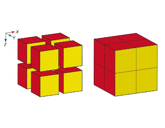
Figure 3: Redundancy elimination. For each subdomain, we only keep the information on faces with a normal along negative axis directions (red), the other faces (yellow) are omitted because they have already been accounted for by adjacent subdomains. After concatenation (dashed line), only the output for faces of the entire grid with normals along the positive axis directions is missing. However, with the margin padded to the molecule when constructing the domain, they do not contain any intersection information to begin with.

2.6 Pipeline

Algorithm 1 provides the pseudocode of the main procedures for the parallelized version of ESES. The function ESES is identical to the original procedure introduced in [14]. Each block (subdomain) uses a unified data structure to store all the necessary information for the part of ESES computation within that block, including the subgrid, the list of relevant atoms, and the output—inside/outside information for grid points and intersection locations on grid edges.

Algorithm 1 ParaESES Algorithm

1:function ParaESES($data,probeRadius,gridSize,margin$)

2:     CreateBlocks($data,blocks$)

3:     for all $b\in blocks$ do in parallel

4:         AssembleRelevantAtoms($b$)

5:         GlobalToLocalIndexMapping($b,bLocal$)

6:         ESES($bLocal,probeRadius,gridSize,margin$)

7:         RemoveDuplicates($bLocal$)

8:         LocalToGlobalIndexMapping($b,bLocal$)

9:         critical

10:              OutputInfo($b$)

11:         end critical

12:     end for

3 Spatial and temporal complexity analysis

Our treatment does reduce the total memory requirement but not the total amount of computation. The number of grid point classification operations to perform, and the number of edge and SES intersection tests are not reduced. Nevertheless, as we divide these task into subdomains of the entire domain, we can either handle the previously intractable problem on a commodity PC with few gigabytes of memory, or greatly reduce the amount of time on a computer cluster or a multi-core computer.

As the number of atoms grows larger or as the resolution becomes finer, the number of grid cells increases asymptotically at $O(whd/h^{3})$, where $h$ is the grid spacing, and $w$, $h$, and $d$ are the width, height, and depth of the bounding box of the molecule respectively. When dealing with large proteins in the original ESES [14] on fine grids, the memory storage is essentially cubic to the number of cells along an edge of the box domain. For instance, a grid with the size of $1000\!\times\!1000\!\times\!1000$ would require roughly $n$ Giga-Byte if each grid point or grid cell requires $n$ Byte storage. As ESES requires the data to reside in the main memory for the grid point classification and grid edge intersection, it cannot fit in the memory of a regular PC, even with virtual memory.

Our straightforward domain decomposition into blocks can effectively shrink the memory footprint, i.e., the maximum memory requirement at any point of the calculation, since all the information required for the localized calculation is associated with the block (or subdomain). No matter how large the original grid size is, we can treat the problem as if it is for the subgrid of size $b_{s}^{3}$, as long as we choose each block to be of size $b_{s}\!\times\!b_{s}\!\times\!b_{s}$. Specifically, there will be $b_{s}^{3}$ grid points to classify, and $3(b_{s}-1)b_{s}^{2}$ grid edges to check for intersections when processing one block. The overhead introduced to handle the boundary of the blocks is negligible, since for each block, there will be $3b_{s}^{2}$ duplicate grid points and $6(b_{s}-1)b_{s}$ duplicate grid edges to check. So in terms of each grid block, there will be an approximate ratio of $O(1/b_{s})$ overhead. As mentioned in the previous section, we introduced a procedure to determine which atoms can influence a particular block, which brings an overhead that is also negligible to the dominating time and space requirement for the grid. This part of the overhead can be further reduced by any spatial data-structure such as a kd-tree, since the construction of the list of atoms within a block is just a query for spatial database entries within a certain spatial range. However, an overly small block size can increase the proportion of the memory the overhead requires, so we do not recommend to aggressively reduce the block size. Fortunately, in practice, even the memory of any modern smart phone can easily accommodate the block size with $b_{s}=32$.

If multi-core machines or clusters with multiple computers are available, one can use our block-based design to achieve essentially a speedup factor controlled by the number of available cores, assuming each core has access to a memory space that can store one block. In an ideal case with infinitely available cores, the time complexity is dropped to $O(b_{s}^{3})$, which is entirely determined by a single block size.

4 Validation and application

We performed our tests on a PC with Intel(R) Xeon(R) CPU E5-1630 v3 @ 3.70GHz and 8GB memory. For parallel computing, we used OpenMP (https://computing.llnl.gov/tutorials/openMP/). We first tested our algorithm on an extremely large multiprotein complex to verify the capability of our algorithm. Then, we analyze the impact of using different block sizes and numbers of threads in terms of the execution time and memory footprint at various grid spacings. Based on the resulting statistics with varying parameter settings, we have confirmed empirically that the memory footprint and execution time indeed behaved as predicted in our analysis above.

All molecular structures used in our validation were downloaded from Protein Data Bank (PDB, https://www.rcsb.org/). The protein-ligand complexes used in our application were obtained from PDBbing (http://www.pdbbind.org.cn/). All structures were processed with pdb-to-xyzr (https://github.com/Pymol-Scripts/Pymol-script-repo/blob/master/modules/MSMS/i64Linux2/pdb_to_xyzr) to assume appropriate van der Waals radii in addition to atomic coordinates.

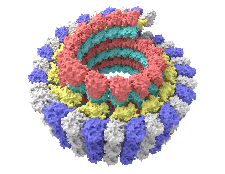
Figure 4: Illustration of the SES generation of multiprotein complex. Here we show the assembly of 3j2u proteins with different chains being marked by different colors. Inner ring: microtubule; intermediate ring: kinesin-13 head domain; and outer ring: curved tubulin protofilament.

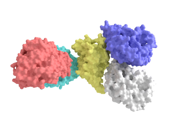
Figure 5: Illustration of the building block protein 3j2u. It shows Drosophila melanogaster kinesin-13 head domain (yellow) binding to tubulin protofilament (silver and blue) and microtubule (red and green).

4.1 Validation on multiprotein complex

In our tests, the algorithm was able to produce the SES successfully for multiprotein complexes with an arbitrary list of atoms at a very high resolution. For instance, Figure 4 shows a multiprotein complex consisting of tubulin, Drosophila melanogaster kinesin-13 KLP10A and microtubule [1] constructed by protein 3j2u with 15575 atoms shown in Figure 5 as the building block. There are 42 such blocks plotted in this multiprotein complex. This typical protein assembly is crucial for investigating the recognition and deformation of tubulins in a microtubule. Due to its excessively large size, such a complex is always an obstacle to handle in theoretical modeling. However, with our software, by only assigning 8 threads to perform the block-based tasks in parallel, the combined memory footprint is controlled to the reasonable amount of 2GB. The whole procedure took about 10 minutes to generate the SES output, including the grid point classification and the intersection information. We were also able to mark different chains in the large protein assembly in the process, with auxiliary information provided by our algorithm, which is the nearby atoms of intersections points. This demonstrates the versatility of our algorithm when used in downstream applications, such as solving the Poisson-Boltzmann equation for electrostatic analysis [13].

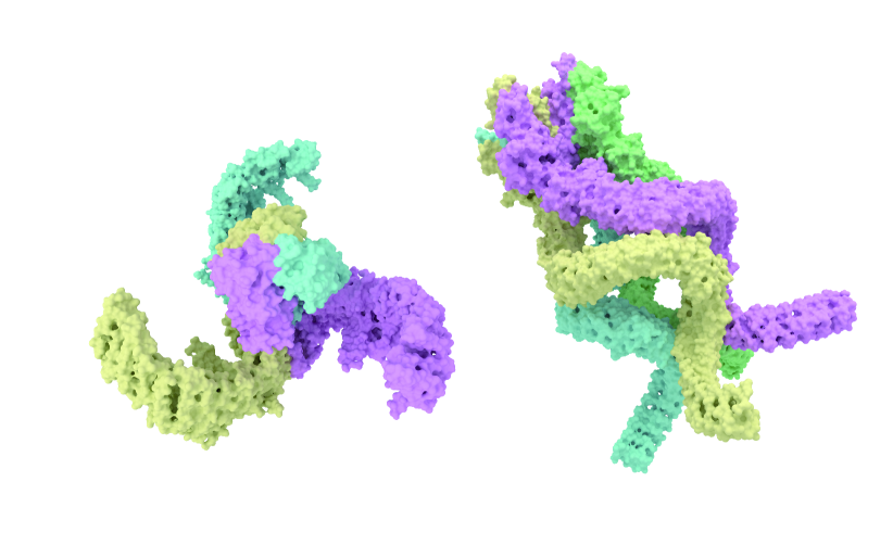
Figure 6: Two models, proteins 5z10 (left) and 5vkq (right), on which tests and statistics of the present algorithm are performed.

4.2 Single-thread analysis

Protein 5z10, shown in Fig. 6 left, reported by [24] is tested as an example for single-thread performance. This protein is a typical mechanosensitive ion channel constructed by three identical blade-like subunits. It is found that by probing the state of surrounding membrane, the channel opens with the distortion of these three blades.

We provide some memory footprint statistics in Figure 7 with only a single thread launched. As the plot indicates, if we do not incorporate the block design and use the original method with the entire grid residing in the memory at all time, the memory footprint increases for fine grids, shown by the curve with circular nodes. If we use blocks with size $b_{s}=128$, the memory footprint drops significantly, simply because only a single block needs to reside in the memory for the single thread, in addition to other auxiliary information, as shown by the curve with square nodes. For the block size $b_{s}=64$, the curve with diamond nodes shows that the memory footprint is further reduced. By assigning blocks, the memory footprint is dominated and restricted by the information stored within a single block, which is controlled only by the block size and is independent of the grid sizes. Therefore, memory footprint of our approach is well-controlled.

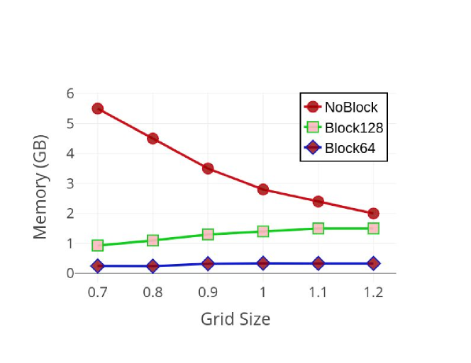
Figure 7: Memory footprint comparison at various grid spacings (Å) for protein 5z10 (single-thread). Curves with circular, square and diamond nodes are corresponding to no block assigned, block size 128 assignment, and block size 64 assignment, respectively.

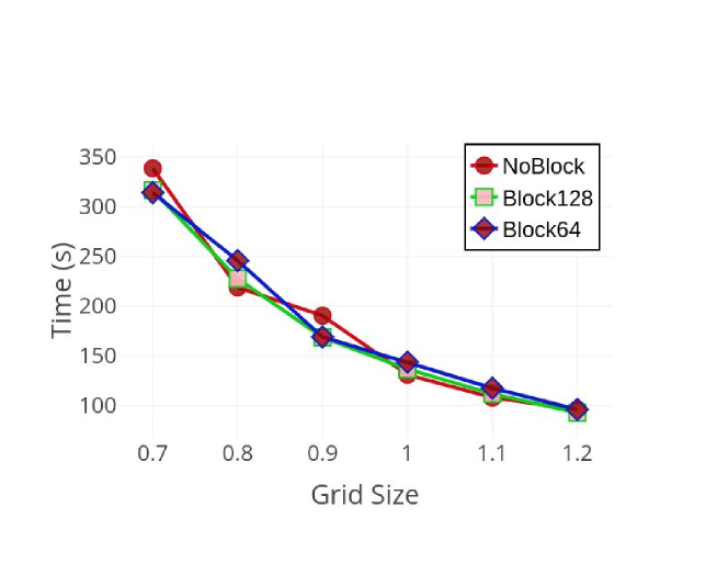
Figure 8: Execution time comparison at various grid spacings (Å) for protein 5z10 (single-thread). Curves with circular, square and diamond nodes are corresponding to no block assigned, block size 128 assignment, and block size 64 assignment, respectively.

The statistics of execution time is provided in Figure 8 for molecule 5z10 with only a single thread. The execution time for different block sizes did not vary significantly. This behavior is expected, since we did not change the total amount of the calculation, for the single-thread version, only the memory footprint is reduced. Note that change was made to the grid point classification or grid edge intersection detection parts. Stated differently, there is no change in analytical nature of the original ESES algorithm.

4.3 Multi-thread analysis

Protein 5vkq, shown in Fig. 6 right, reported by [11] is used as an example to test multi-thread performance. This protein is a typical mechanosensitive ion channel in bacteria. Its long and spring shaped domains are tethered with microtubules, which will open when it senses the motion of the cytoskeleton environment.

If we initiate $N$ threads in parallel, we expect that the memory footprint is roughly $N$ times the numbers when the number of $N$ is large. In practice, we observed that it is actually smaller due to that some of the overhead is shared by the threads, especially when $N$ is small. In Figure 9, we present the statistics of memory footprint for protein 5vkq with 8 threads launched in parallel. The curve with circular nodes serves as a baseline when we stick to the original ESES algorithm, which shows an excessive memory requirement. When launching 8 threads, obviously the memory footprint shifted higher compared to launching a single thread simply because we need to load the execution context for all 8 blocks. Nevertheless the memory footprint is still significantly reduced compared to the baseline, unless the number of threads matches the number of blocks. In addition, we still control the memory footprint by the number of threads launched. The curve with square nodes shows the memory usage with block size $b_{s}=128$, and the curve with diamond nodes shows the case with block size $b_{s}=64$.

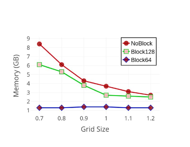
Figure 9: Memory footprint comparison at various grid spacings (Å) for protein 5vkq (8-threads). Curves with circular, square and diamond nodes are corresponding to no block assigned, block size 128 assignment, and block size 64 assignment, respectively.

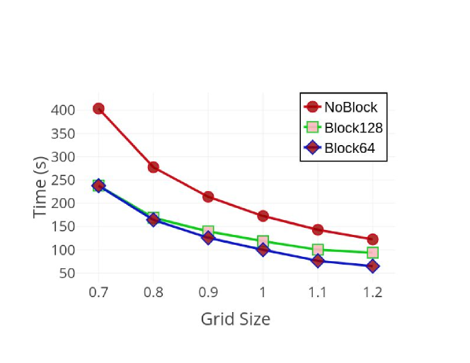
Figure 10: Execution time comparison at various grid spacings (Å) for protein 5vkq (8-threads). Curves with circular, square and diamond nodes are corresponding to no block assigned, block size 128 assignment, and block size 64 assignment, respectively.

The execution time statistics for the same 8-thread experiment for protein 5vkq are shown in Figure 10. The curve with circular nodes gives us a baseline when we stick to the original ESES algorithm. In this example, the execution time was reduced significantly simply by launching several threads at the same time. It is not a perfect 8-times improvement, as predicted by Amdahl’s Law [15], because there are always critical sections that need serial execution such as file I/O. We also found that a smaller block size (curve with diamond nodes) also brings some additional improvements as in the single-thread mode. It is most likely due to the same reason that the memory allocation is easier for smaller blocks. Taking into account both the spatial and temporal statistics, we observed that by reducing the block size, we can significantly reduce the memory footprint without any negative impact on the time performance and algorithm accuracy.

Finally, we apply the present approach to a large set of protein-ligand complexes. We consider the PDBbing v2016 core set of 290 protein-ligand complexes. Our results in terms of grid dimension, block dimension, surface area, and surface enclosed volume are given for each protein in Appendix LABEL:apdx:list. These results can be used by independent researchers to validate their own surface generations. The computational parameters are set to probe size 1.4Å, grid spacing 0.4Å, grid extension 0.8Å  and block size 64. Note that the proposed method has no effect on the ESES generation quality. The proposed method can thus be used as an efficient replacement to ESES, and be applied to any solvent excluded surface based molecular modeling and analysis.

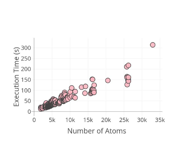
Figure 11: Execution time analysis. The scatter plot of execution time vs the number of atoms is given for 290 proteins when 8 threads are used.

5 Conclusion

We present a divide-and-conquer approach to solve the memory explosion issue when dealing with large macromolecules at high grid resolutions. The approach is based on the localized nature of the computations involved in Eulerian solute-excluded surfaces (ESESs) [14]. In the present approach, we partition the entire computational domain into subdomains (blocks) that can fit into a given size of memory space. The memory requirement is determined by the data in the block(s) used in the current calculation. In this manner, we can control the upper bound of the memory footprint, and allow the user to run our software on a typical commodity personal computer (PC). Taking the advantage of the locality, we also incorporate the power of parallel computing to further enhance the performance. With such a practical implementation, we can significantly extend the applicability of the earlier ESES algorithm by lifting its constraints of memory requirements and running on a single CPU. The present improvement does not change the analytical nature of the original ESES algorithm. The proposed method is validated on the ESES generation of an excessively large protein complex and a couple of large proteins. Application is considered to 290 protein-ligand complexes.

There is still a room for further improvements. In the potential analytical patch construction, especially for the saddle and concave patches, we simply consider all possible pairs of atoms which are at a distance below a threshold determined by the van der Waals radii. Apparently, there is a redundancy in such an approach, since some patches are buried inside the molecular surface and may be pre-culled to save computation. As future work, we wish to explore fast calculations that can eliminate such patches before classifying grid points. Another direction to explore is to consider GPU computing, since a similar parallelized design can be applied when mapping them to GPU threads and blocks instead of CPU cores. A central issue in carrying out a GPU implementation is how the analytical SES patch construction and the associated high order polynomial root finding at grid edge and surface intersection can be efficiently adapted to the less powerful ALU units on GPUs. Further simplifications may be desirable to harness the power of GPU for this problem.

Appendix A Surface generation test

Table 1: Surface generation results of the PDBbing v2016 core set sorted by the number of atoms.

Protein ID	#Atoms	Grid Dim	Block Dim	Area(Å2)	Volume(Å3)	time($s$)
3dxg	1856	105x101x117	2x2x2	5777.88	16569.2	13.0162
3d6q	1856	105x102x117	2x2x2	5793.47	16601.3	19.8521
1w4o	1856	105x99x116	2x2x2	5776.42	16575.4	14.2584
1o0h	1856	104x108x117	2x2x2	5753.33	16456.4	14.2019
1u1b	1856	103x129x94	2x3x2	5790.07	16722.8	12.3264
4lzs	2121	95x132x127	2x3x2	6585.37	18644.5	19.2717
3u5j	2121	95x135x127	2x3x2	6686.26	18677.5	17.7138
4wiv	2121	138x85x125	3x2x2	6749.24	18694.1	16.3995
4ogj	2121	129x110x110	3x2x2	6710.66	18851.7	16.8964
3p5o	2121	96x135x125	2x3x2	6718.7	18764.6	17.1206
3lka	2408	110x112x101	2x2x2	7040.19	21685.7	16.9318
3ehy	2408	110x112x100	2x2x2	7039.49	21574.7	15.2638
3nx7	2408	112x112x101	2x2x2	6960.15	21681.9	14.4231
3tsk	2425	109x100x119	2x2x2	7057.27	22082.1	14.6475
4gr0	2425	109x101x115	2x2x2	6962.62	21868.1	15.4103
3nq9	2584	120x120x112	2x2x2	7368.2	23464	22.7301
5aba	3025	111x126x136	2x2x3	8747.75	27568.7	25.6786
4agq	3025	113x126x138	2x2x3	8885.8	27571.7	19.5389
5a7b	3047	111x130x136	2x3x3	8943.39	27637.8	27.9725
4agp	3047	114x126x138	2x2x3	8877.19	27718.7	27.5211
4agn	3069	112x126x137	2x2x3	8966.61	27884.4	29.8699
2qnq	3128	104x139x143	2x3x3	8577.43	27855.4	20.697
3cyx	3128	106x134x142	2x3x3	8566.31	27591.5	21.0516
1eby	3134	107x136x147	2x3x3	8604.66	28389.9	21.5876
3o9i	3134	152x103x111	3x2x2	8526.46	27838	19.3083
1a30	3138	107x136x140	2x3x3	8459.42	27734.2	32.6073
4abg	3204	109x118x135	2x2x3	8104.51	29113.2	27.3888
1uto	3220	123x99x132	2x2x3	8037.53	29010	17.8095
3gy4	3220	123x107x133	2x2x3	7993.9	29061.3	20.5542
1k1i	3220	124x108x131	2x2x3	8127.1	29250	20.144
1o3f	3220	121x132x111	2x3x2	8059.72	29193.8	19.3656
3kr8	3248	140x132x106	3x3x2	9356.53	29196.6	20.4359
2yki	3259	122x124x126	2x2x2	9171.29	29287.1	19.6484
4kzq	3278	137x130x103	3x3x2	9356.27	29733.6	19.8373
4kzu	3278	139x131x108	3x3x2	9308.97	29802.4	20.4075
4j21	3292	149x125x107	3x2x2	9533.27	30100.4	20.4142
4j3l	3292	125x150x106	2x3x2	9398.54	29849.4	19.9642
1yc1	3313	119x110x129	2x2x3	9072.47	29432.3	20.9225
3ozt	3357	200x148x114	4x3x2	10015	30240.5	40.6189
3ozs	3357	196x150x114	4x3x2	9996.25	30152.6	26.3215
3oe5	3357	193x149x113	4x3x2	9925.33	30107	27.2306
3oe4	3357	193x149x114	4x3x2	9980.64	30163	27.2095
3nw9	3365	107x115x144	2x2x3	8131.95	30170.6	19.38
3b27	3388	128x126x159	3x2x3	9731.4	30503.3	24.2988
2fxs	3409	151x128x132	3x3x3	9203.98	30434.6	23.9637
2yge	3420	151x130x134	3x3x3	9285.46	30724.4	27.1157
2iwx	3426	155x129x133	3x3x3	9345.14	30760.3	27.0977
2vw5	3426	157x129x134	3x3x3	9341.02	30901.6	28.3237
3rlr	3449	121x121x156	2x2x3	9914.87	30865.4	23.8025
1lpg	3665	125x136x114	2x3x2	9706.24	32892.4	20.5021
4crc	3711	127x120x141	2x2x3	9907.48	33608.9	22.8678
4x6p	3715	140x116x126	3x2x2	10131.4	33827.4	20.8315
4cra	3724	145x128x115	3x3x2	9972.72	33624	22.1204
4ty7	3727	133x138x144	3x3x3	10136.1	33908.5	24.43
3kgp	3737	144x112x123	3x2x2	9519.34	33612.6	23.194
1o5b	3810	146x127x120	3x2x2	9445.63	34582.3	22.1093
1c5z	3811	146x129x120	3x3x2	9531.12	34644.1	33.7694
1sqa	3818	128x157x125	3x3x2	10141.1	35162.1	23.7716
1owh	3820	127x156x125	2x3x2	10149.2	35375.6	23.6066
4qd6	3849	134x147x211	3x3x4	12029.2	35089.4	33.5549
3qgy	3896	133x135x159	3x3x3	10853.7	35113.4	28.1767
4de2	3900	138x109x147	3x2x3	9295.39	34595.6	35.9985
4de3	3900	138x111x144	3x2x3	9241.18	34660.7	23.651
1z95	3917	141x120x156	3x2x3	10169.7	35038.8	27.3216
4de1	3923	139x108x152	3x2x3	9427.62	34862.4	23.8837
3g2z	3925	140x109x152	3x2x3	9285.38	34891.5	22.2739
3g31	3925	140x110x147	3x2x3	9326.88	34989	26.6228
4rfm	3942	138x128x154	3x3x3	10899.5	35830	25.4256
3kwa	4032	127x125x150	2x2x3	10003.9	36326.8	35.8207
4jsz	4048	127x124x149	2x2x3	10121.1	36590	22.4405
3ryj	4054	129x123x148	3x2x3	10333.2	36435.3	23.7567
3b68	4068	149x120x158	3x2x3	10827.6	36233.7	29.5425
3b5r	4068	149x120x159	3x2x3	10866.6	36325.1	28.6952
3b65	4068	149x120x158	3x2x3	10801	36251.7	28.1824
2weg	4071	128x121x147	3x2x3	10146	36513.5	24.3336
3dd0	4071	130x123x149	3x2x3	10322.6	36951.8	23.7389
3gbb	4086	123x149x157	2x3x3	11431.4	36652.7	27.8599
3g0w	4099	153x124x150	3x2x3	10647.3	36712.6	27.9932
3fv2	4101	145x134x121	3x3x2	11330.7	36688	24.859
3fv1	4101	145x140x122	3x3x2	11270.2	36526.1	24.8372
3fur	4161	133x110x172	3x2x3	11796.3	37539	25.4867
3myg	4169	156x145x126	3x3x2	11063	37469.2	27.555
4m0y	4177	131x152x148	3x3x3	11990.4	38728.9	29.0143
3u9q	4179	124x131x154	2x3x3	11740	37330.8	33.5672
3jvs	4186	139x118x183	3x2x3	11445	37468.2	27.3559
4m0z	4199	128x148x149	3x3x3	11655.2	38361.3	30.2577
3ao4	4210	137x133x144	3x3x3	10992	38287.1	26.372
3jvr	4218	138x116x181	3x2x3	11495.1	37840.2	24.8808
3b1m	4229	116x129x169	2x3x3	11722.6	37809.4	27.7153
3mss	4263	131x118x172	3x2x3	12047.8	38810.3	38.2454
2c3i	4274	154x144x123	3x3x2	11301.2	38876.8	26.4624
2yfe	4281	139x156x153	3x3x3	11923.7	38510.9	31.6776
3pyy	4289	111x128x166	2x3x3	11972.6	38784.4	25.2828
1nvq	4291	139x124x181	3x2x3	11909.9	38394.9	28.3015
2xbv	4291	149x135x131	3x3x3	11794.8	39406.4	27.6058
4twp	4292	165x147x113	3x3x2	11511.7	38978.3	27.6603
3bgz	4318	158x141x121	3x3x2	11265.8	39021.6	28.2811
2wtv	4337	118x161x160	2x3x3	11713	38572.4	27.7694
2v7a	4340	129x136x166	3x3x3	12063.1	39932	28.3806
1mq6	4372	167x139x112	3x3x2	11625.3	39651.5	26.7912
3uo4	4392	157x142x139	3x3x3	11569.5	39341.1	32.1715
3up2	4392	158x145x139	3x3x3	11612.7	39524.3	31.3933
5dwr	4397	135x151x134	3x3x3	11467.8	40084.1	27.2752
3jya	4408	134x155x133	3x3x3	11571	40232.4	27.4488
1z6e	4413	164x142x109	3x3x2	11656.5	39643.9	25.5687
2brb	4425	141x133x182	3x3x3	12414	40414.9	31.3865
2br1	4425	138x135x183	3x3x3	12257.1	39755.9	32.0098
3utu	4434	128x130x139	3x3x3	11221.5	39829.2	24.9517
2y5h	4440	140x168x116	3x3x2	12126	40601.4	26.7111
1bcu	4446	128x129x140	3x3x3	11130.7	40337.1	37.4077
4k18	4453	161x141x132	3x3x3	11652.3	40461.1	28.9929
1oyt	4479	129x132x140	3x3x3	11485.2	40270.1	26.678
2zda	4513	131x131x143	3x3x3	11344.7	40606	27.9352
4k77	4549	146x142x150	3x3x3	12696.8	41470.2	30.1223
4cig	4564	144x125x152	3x2x3	12304.1	41078.4	40.9304
3k5v	4588	143x184x124	3x3x2	13284.3	41730.7	29.958
3bv9	4621	138x138x136	3x3x3	11636.2	41530.9	27.8745
3zt2	4642	142x131x155	3x3x3	12440.7	41627.9	32.2067
3zsx	4642	144x130x153	3x3x3	12556.8	41830	45.4165
2zy1	4646	149x144x159	3x3x3	12283.4	41678.4	31.8607
3uri	4650	147x152x134	3x3x3	11386.5	42463.2	29.2076
2fvd	4653	140x114x170	3x2x3	12820	41544.9	30.1102
2v00	4669	139x127x166	3x2x3	11462.2	42410.6	42.6454
3wz8	4669	140x127x167	3x2x3	11460.9	42536.5	27.7162
3pww	4669	138x126x166	3x2x3	11500.2	42377.7	30.2387
3prs	4669	139x125x166	3x2x3	11499.9	42426.3	28.767
3zso	4670	143x132x153	3x3x3	12690	41991.9	31.6446
4ea2	4670	148x144x161	3x3x3	12343.4	42173	32.4862
2zcr	4670	149x147x160	3x3x3	12337	41938.9	33.0923
4hge	4674	161x156x143	3x3x3	13043.1	42660	33.0706
4ivd	4698	214x143x158	4x3x3	13788.6	42619.9	40.4818
3fcq	4700	173x131x132	3x3x3	10956.1	42376.4	34.77
1z9g	4700	175x132x133	3x3x3	11019.2	42836.4	29.4944
1qf1	4700	173x132x132	3x3x3	10908.5	42623.9	28.7241
4ivb	4713	215x143x158	4x3x3	13772.8	42947.1	41.5465
4ivc	4713	213x142x158	4x3x3	13712.4	42361	40.4934
3acw	4714	150x146x161	3x3x3	12637.4	42325.7	48.4493
2zcq	4714	145x143x157	3x3x3	12308.2	42281.4	31.2949
4f09	4739	143x159x169	3x3x3	13163	42812.4	35.2086
4gfm	4762	145x148x129	3x3x3	12925.4	43402.4	28.8006
1pxn	4788	142x114x170	3x2x3	13001.5	42799.9	30.9308
2hb1	4811	170x145x117	3x3x2	11635.3	43180.8	45.4613
1bzc	4811	173x142x115	3x3x2	11505.4	43489.1	30.1936
2qbq	4811	170x145x118	3x3x2	11678.6	43351.1	31.5649
2qbp	4811	169x145x117	3x3x2	11655.4	43424.7	31.878
2xnb	4819	141x111x171	3x2x3	12885.2	43258.1	29.5643
2qbr	4830	177x145x120	3x3x2	11737.8	43724.4	30.8117
3e5a	4850	152x161x145	3x3x3	13072.8	43625.6	32.6783
4e6q	4869	168x138x181	3x3x3	13820.9	43831.2	37.587
4jia	4878	142x183x165	3x3x3	14222.9	44267.3	37.1466
3pxf	4908	157x110x180	3x2x3	13841.6	43820.6	43.9436
3uuo	4922	145x150x157	3x3x3	12998.8	45572.7	31.3175
3ueu	4966	123x130x203	2x3x4	13255.2	44763.8	32.4677
3uew	5000	123x128x213	2x3x4	13666.4	45435.3	33.8787
3twp	5009	164x127x133	3x2x3	12462.3	45286.2	45.8088
3qqs	5009	134x166x147	3x3x3	12412.7	45349.6	31.8109
3uev	5068	125x128x201	2x3x4	13640.4	45616.3	31.0619
3ui7	5091	142x151x157	3x3x3	13135.4	46772.9	32.3145
3uex	5096	124x129x209	2x3x4	13975.3	46266	32.1042
5c2h	5191	151x147x149	3x3x3	13072.6	47126.9	35.0963
5c1w	5235	147x156x157	3x3x3	13216.2	47644.6	36.0221
5c28	5235	148x154x154	3x3x3	13159.3	47569.4	32.2369
3ag9	5267	137x174x143	3x3x3	13473.3	47423.8	36.549
4w9h	5271	174x143x199	3x3x4	14645.7	47401.8	41.345
4msc	5280	147x158x158	3x3x3	13787.5	48439.7	34.8642
4w9c	5282	175x145x200	3x3x4	14685.8	47924.2	58.7774
4w9l	5282	174x145x197	3x3x4	14812.9	47975.6	41.5329
4w9i	5282	177x143x199	3x3x4	14614.3	47854.5	40.2372
4bkt	5296	141x179x201	3x3x4	14714.9	48335	57.7965
4llx	5299	150x159x157	3x3x3	13540.6	48052.3	38.9411
4mrw	5299	150x159x157	3x3x3	13525.4	48193.6	50.8482
4mrz	5299	149x160x156	3x3x3	13504.9	47956.9	52.8705
4msn	5299	150x159x155	3x3x3	13688.1	48625.8	51.905
4dli	5411	185x140x133	3x3x3	15130.5	49108.4	36.0334
4f9w	5433	185x140x129	3x3x3	14761.8	48989.7	33.0079
2zb1	5575	155x149x155	3x3x3	15142.3	50414.7	37.3719
3gv9	5581	153x144x145	3x3x3	12928.2	50191.6	33.2439
3gr2	5581	153x140x144	3x3x3	12961.9	50214	35.9617
4kz6	5581	151x156x133	3x3x3	12812.9	49828.8	48.0046
4jxs	5581	151x157x134	3x3x3	13053.9	50220.6	47.9802
2r9w	5581	154x141x143	3x3x3	13174	49905.5	34.4525
3e93	5584	156x156x159	3x3x3	15401.5	50252.8	39.2194
1r5y	5595	146x134x181	3x3x3	13256.5	50372	36.9078
3e92	5609	156x152x158	3x3x3	15307	50559.2	38.9401
1s38	5650	146x132x179	3x3x3	13268	50828.2	36.4457
1ydr	5813	136x178x129	3x3x3	14353.4	52608.3	34.2593
1ydt	5813	136x177x129	3x3x3	14423	52672.4	33.32
3rsx	5833	154x178x132	3x3x3	14770.9	54165.6	54.6174
1q8t	5875	141x186x138	3x3x3	15349.5	54420.4	53.2045
1q8u	5928	141x187x134	3x3x3	15888.7	55111.5	36.2449
4gid	5997	160x173x150	3x3x3	14746.3	54907.2	41.5304
2vkm	6019	160x175x149	3x3x3	14775.8	54738.4	41.6591
4djv	6034	166x149x174	3x3x3	14975.7	55246.1	42.4239
3udh	6111	166x182x131	3x3x3	15607.2	55890.3	42.4351
3wtj	6504	197x116x177	4x2x3	18210.3	58882.8	39.4775
2xdl	6560	131x191x125	3x4x2	17346.2	59278	48.6823
2qe4	6651	172x149x145	3x3x3	16615.2	59904.7	39.4594
2wer	6846	129x223x147	3x4x3	17262.1	61418.2	42.2958
4f3c	6854	200x136x128	4x3x3	14854	62181.4	40.3111
1nc3	6896	167x108x189	3x2x3	15249.6	61913	39.4786
1nc1	6905	168x106x190	3x2x3	15224.4	62500	37.7971
1y6r	6905	169x107x191	3x2x4	15335.1	62804.4	37.6239
4f2w	6979	109x145x201	2x3x4	15692.2	63726.8	37.0809
2cet	7025	156x147x148	3x3x3	14613.8	63522.8	41.3852
4jfs	7054	157x181x185	3x3x3	16911.8	63804.5	48.7066
4j28	7054	157x184x184	3x3x3	17110.9	64082	46.2038
2xii	7054	160x148x195	3x3x4	16914	64003.5	44.4223
2j7h	7066	155x149x149	3x3x3	14854.5	64039.6	42.2341
4pcs	7076	188x174x177	3x3x3	17301.3	64169.7	49.6077
2cbv	7141	162x161x150	3x3x3	14978.2	64682.5	46.0519
2j78	7142	163x153x156	3x3x3	15058.2	64684	47.1593
2pog	7210	161x174x166	3x3x3	18032.6	64766.2	46.4577
4cr9	7448	213x142x171	4x3x3	19486.5	67552.5	67.7259
2p4y	7688	192x177x185	4x3x3	20497.6	69126.1	55.2999
4mgd	7695	167x173x185	3x3x3	19584.2	69673.7	75.4981
1vso	7794	173x213x149	3x4x3	20774.4	69624.7	71.1788
2p15	7849	172x166x189	3x3x3	19652.8	71004.1	50.9455
1qkt	8026	184x199x165	3x4x3	21676	72259.2	56.2978
4mme	8118	157x182x161	3x3x3	17939	73566.5	52.593
1p1q	8134	188x174x146	3x3x3	20746	72655.6	52.0299
1p1n	8134	191x188x149	4x3x3	21060.8	72683.9	55.3808
4dld	8158	172x162x182	3x3x3	21683.9	73727	50.1094
4u4s	8162	194x214x155	4x4x3	21407.1	73234.4	68.8114
1syi	8170	159x151x182	3x3x3	21317.4	73091.7	47.9248
2al5	8186	148x199x191	3x4x4	21975.7	73709.8	54.9643
1h23	8286	174x168x164	3x3x3	18128.9	75779.4	49.7802
1h22	8296	174x168x159	3x3x3	17949.9	76064.8	50.8137
1gpk	8301	170x171x166	3x3x3	18075.1	75389.9	52.4765
1gpn	8303	171x171x161	3x3x3	18205.4	75497	51.2762
3coy	8382	171x162x236	3x3x4	21615.4	75471.6	56.5176
3ivg	8393	171x164x225	3x3x4	21473.8	75420.7	77.236
3coz	8472	171x163x236	3x3x4	21908.6	76264.1	55.5484
3aru	8474	258x145x182	5x3x3	19817.1	77814.7	90.0987
4ddh	8495	168x163x226	3x3x4	21761.8	76872.6	83.0679
4ddk	8519	169x164x236	3x3x4	21986.4	76989.4	54.1794
3arp	8549	249x158x177	4x3x3	20026.1	78534	58.3026
3arv	8563	249x158x178	4x3x3	20188.7	78669.3	56.6699
3ary	8563	249x159x176	4x3x3	20110.6	78665.2	58.0375
3arq	8563	249x158x177	4x3x3	20159.2	78685.2	59.7228
4eo8	8692	161x174x194	3x3x4	21052	78285.7	55.5408
4ih7	8701	164x173x198	3x3x4	20699.9	79327.2	53.9337
4ih5	8703	168x173x196	3x3x4	20942.1	79392	77.9905
3cj4	8720	174x168x193	3x3x4	21129.3	78945.2	56.0903
3gnw	8738	162x166x201	3x3x4	20977.2	78570.2	53.2703
4eor	8949	165x203x190	3x4x3	21622.7	82242.2	57.4209
4e5w	9243	234x238x156	4x4x3	25469.5	84609.8	69.0594
2wca	9295	232x207x176	4x4x3	21978.8	84461.4	67.2198
2w4x	9306	230x207x177	4x4x3	21814.6	83862	64.4236
5tmn	9400	213x184x178	4x3x3	21020.7	86484.7	58.6322
4tmn	9400	213x184x178	4x3x3	21224.8	85989	58.9291
3r88	9948	203x241x214	4x4x4	23584.2	90457.6	81.9614
4gkm	10018	234x134x241	4x3x4	23776.8	90996.8	65.9909
4owm	10046	217x157x239	4x3x4	23757.2	90913.7	92.6124
2w66	10441	198x259x184	4x5x3	24986.9	93973	111.381
2vvn	10458	199x259x185	4x5x3	24967.8	94680.3	72.0086
3ge7	11112	212x130x232	4x3x4	24214.1	100795	68.4804
3gc5	11402	210x131x233	4x3x4	24774	102959	65.0512
3rr4	11416	210x132x231	4x3x4	24687.2	102504	94.0242
3g2n	13194	212x195x213	4x4x4	29288.2	122132	114.925
2wvt	14130	181x167x298	3x3x5	32575.7	128126	86.4621
2wbg	14288	253x208x176	4x4x3	28560.6	129288	118.505
3zdg	15709	206x200x214	4x4x4	38866	144437	85.0419
3u8n	15960	189x211x224	3x4x4	40327.3	147464	88.1512
3u8k	16004	178x208x212	3x4x4	41707.7	149056	87.3808
2xys	16045	233x229x215	4x4x4	40437	146928	100.344
1ps3	16157	205x213x246	4x4x4	33802.4	148038	94.0591
3dx1	16185	204x212x251	4x4x4	33359.3	147934	152.277
3d4z	16185	205x211x248	4x4x4	33016.8	147051	100.968
3dx2	16185	206x215x246	4x4x4	33246.5	147399	106.006
3ejr	16185	205x213x248	4x4x4	33829.1	148567	106.539
3f3a	16252	232x181x258	4x3x5	34144.4	144819	151.338
3f3c	16364	233x194x252	4x4x4	34288.8	147783	104.871
3f3d	16364	235x194x254	4x4x5	34513.1	149136	104.439
3f3e	16364	233x193x253	4x4x4	34231.4	147296	102.979
2wn9	16453	209x212x199	4x4x4	42401.8	150607	92.4032
4qac	16464	197x215x214	4x4x4	41359.3	151072	90.1083
2wnc	16628	231x210x223	4x4x4	42586.5	153057	99.1218
2x00	16661	212x214x201	4x4x4	43256.1	154206	90.0651
1e66	16692	288x256x222	5x5x4	36312.4	153168	124.091
2xj7	20502	207x307x309	4x5x5	48182.4	186415	146.431
3n7a	25763	233x248x260	4x4x5	54932.7	236584	211.186
4ciw	25848	266x266x266	5x5x5	55675.4	236737	164.345
2xb8	25848	263x263x263	5x5x5	56332.5	236229	160.274
3n86	25889	233x239x237	4x4x4	54431	236562	126.98
3syr	26110	217x217x311	4x4x5	56471.3	243244	146.197
3l7b	26188	218x218x312	4x4x5	56457.9	244430	149.303
4eky	26216	217x217x311	4x4x5	56276.4	244775	217.654
3ebp	26216	216x216x311	4x4x5	55922.4	243389	143.218
3n76	26220	264x264x264	5x5x5	54813.3	237610	161.143
2ymd	32988	357x324x204	6x6x4	79086.5	303394	314.233

References

- [1] Ana B Asenjo, Chandrima Chatterjee, Dongyan Tan, Vania DePaoli, William J Rice, Ruben Diaz-Avalos, Mariena Silvestry, and Hernando Sosa. Structural model for tubulin recognition and deformation by kinesin-13 microtubule depolymerases. Cell reports, 3(3):759–768, 2013.
- [2] P. W. Bates, Z. Chen, Y. H. Sun, G. W. Wei, and S. Zhao. Geometric and potential driving formation and evolution of biomolecular surfaces. J. Math. Biol., 59:193–231, 2009.
- [3] PW Bates, Guo-Wei Wei, and Shan Zhao. Minimal molecular surfaces and their applications. Journal of Computational Chemistry, 29(3):380–391, 2008.
- [4] J. Blinn. A generalization of algebraic surface drawing. ACM Transactions on Graphics, 1(3):235–256, 1982.
- [5] Minxin Chen and Benzhuo Lu. Tmsmesh: A robust method for molecular surface mesh generation using a trace technique. J Chem. Theory and Comput., 7:203–212, 2011.
- [6] Ho-Lun Cheng and Xinwei Shi. Quality mesh generation for molecular skin surfaces using restricted union of balls. Computational Geometry, 42:196–206, 2009.
- [7] Michael L Connolly. Solvent-accessible surfaces of proteins and nucleic acids. Science, 221(4612):709–713, 1983.
- [8] S. Decherchi and W. Rocchia. A general and Robust Ray-Casting-Based Algorithm for Triangulating Surfaces at the Nanoscale. PLoS ONE, 8:e59744, 2013.
- [9] B. S. Duncan and A. J. Olson. Shape analysis of molecular surfaces. Biopolymers, 33:231–238, 1993.
- [10] J Dzubiella, Jessica MJ Swanson, and JA McCammon. Coupling hydrophobicity, dispersion, and electrostatics in continuum solvent models. Physical review letters, 96(8):087802, 2006.
- [11] Peng Jin, David Bulkley, Yanmeng Guo, Wei Zhang, Zhenhao Guo, Walter Huynh, Shenping Wu, Shan Meltzer, Tong Cheng, Lily Yeh Jan, et al. Electron cryo-microscopy structure of the mechanotransduction channel nompc. Nature, 547(7661):118, 2017.
- [12] Byungkook Lee and Frederic M Richards. The interpretation of protein structures: estimation of static accessibility. Journal of molecular biology, 55(3):379–IN4, 1971.
- [13] Lin Li, Joshua Alper, and Emil Alexov. Multiscale method for modeling binding phenomena involving large objects: application to kinesin motor domains motion along microtubules. Scientific reports, 6:23249, 2016.
- [14] Beibei Liu, Bao Wang, Rundong Zhao, Yiying Tong, and Guo-Wei Wei. ESES: Software for Eulerian solvent excluded surface. Journal of Computational Chemistry, 38(7):446–466, 2017.
- [15] Michael D McCool, Arch D Robison, and James Reinders. Structured parallel programming: patterns for efficient computation. Elsevier, 2012.
- [16] K. Opron, K. L. Xia, and G. W. Wei. Fast and anisotropic flexibility-rigidity index for protein flexibility and fluctuation analysis. Journal of Chemical Physics, 140:234105, 2014.
- [17] Frederic M Richards. Areas, volumes, packing, and protein structure. Annual review of biophysics and bioengineering, 6(1):151–176, 1977.
- [18] Timothy J Richmond. Solvent accessible surface area and excluded volume in proteins: Analytical equations for overlapping spheres and implications for the hydrophobic effect. Journal of molecular biology, 178(1):63–89, 1984.
- [19] W. Rocchia, S. Sridharan, A. Nicholls, E Alexov, A Chiabrera, and B. Honig. Rapid grid-based construction of the molecular surface and the use of induced surface charge to calculate reaction field energies: Applications to the molecular systems and geometric objects. Journal of Computational Chemistry, 23:128 – 137, 2002.
- [20] Michel F Sanner, Arthur J Olson, and Jean-Claude Spehner. Reduced surface: an efficient way to compute molecular surfaces. Biopolymers, 38(3):305–320, 1996.
- [21] Guo-Wei Wei. Differential geometry based multiscale models. Bulletin of mathematical biology, 72(6):1562–1622, 2010.
- [22] K. L. Xia, K. Opron, and G. W. Wei. Multiscale multiphysics and multidomain models — Flexibility and rigidity. Journal of Chemical Physics, 139:194109, 2013.
- [23] Z. Y. Yu, M. Holst, Y. Cheng, and J. A. McCammon. Feature-preserving adaptive mesh generation for molecular shape modeling and simulation. Journal of Molecular Graphics and Modeling, 26:1370–1380, 2008.
- [24] Qiancheng Zhao, Heng Zhou, Shaopeng Chi, Yanfeng Wang, Jianhua Wang, Jie Geng, Kun Wu, Wenhao Liu, Tingxin Zhang, Meng-Qiu Dong, et al. Structure and mechanogating mechanism of the piezo1 channel. Nature, 554(7693):487, 2018.
- [25] Q. Zheng, S. Y. Yang, and G. W. Wei. Molecular surface generation using PDE transform. International Journal for Numerical Methods in Biomedical Engineering, 28:291–316, 2012.