Concurrent Robin Hood Hashing

Abstract.

In this paper we examine the issues involved in adding concurrency to the Robin Hood hash table algorithm. We present a non-blocking obstruction-free K-CAS Robin Hood algorithm which requires only a single word compare-and-swap primitive, thus making it highly portable. The implementation maintains the attractive properties of the original Robin Hood structure, such as a low expected probe length, capability to operate effectively under a high load factor and good cache locality, all of which are essential for high performance on modern computer architectures. We compare our data-structures to various other lock-free and concurrent algorithms, as well as a simple hardware transactional variant, and show that our implementation performs better across a number of contexts.

1. Introduction

Concurrent data-structures allow multiple threads to operate on them without risk of data corruption, as well as providing guarantees of correctness for concurrent operations. Lock-free data-structures are a class of concurrent data-structures that have specific properties relating to system or thread progress guarantees. The programming of portable and practical lock-free data-structures is becoming ever more practical, with the addition of mainstream language support for atomic variables, and a well defined thread memory model (see [5], [28]).

Concurrent algorithms can be separated into two major classes, namely blocking and non-blocking, with both featuring further partitions based on the specific progress guarantees within those classes [20]. Blocking algorithms have well documented issues when it comes to their use. They are susceptible to deadlock, priority inversion, convoying, and a lack of composability with respect to multiple operations on data-structures. A lock-free, or non-blocking, algorithm has none of these problems. Such algorithms suffer, however, from their own set of challenges relating to memory management ([1], [2], [26], [14], [9]), correctness ([22], [24], [3]) and potentially lackluster performance as the system is flooded with contention under heavy write load. As hardware manufacturers resort to expanding processor core counts for enhanced performance [34], non-blocking data-structures are coming to the fore, providing more robust progress guarantees and tolerance to the suspension of threads. For end consumers to realise the full performance of their system, algorithms must efficiently exploit as many cores as possible.

Hash tables are one of the major building blocks in software applications, providing efficient implementations for the abstract data types of maps and sets. These data-structures are highly versatile, making them an active area of research in concurrency (e.g. [25], [20], [21], [8], [27], [30], [32]). Hash tables are associative data-structures that contain a pool of keys and associated values [10], lending themselves to efficient implementations. In general, they feature the methods Add, Remove, and Contains, each of which is bound by $\mathcal{O}(1)$ computational complexity while requiring $\mathcal{O}(n)$ space [10]. Hash table algorithms achieve this performance by calculating an index, called a hash, from each key, and use this to efficiently find the relevant entry in the pool of keys, normally an array. Unlike comparative structures, which store keys in a sorted order and binary search through the space, hash tables rely on the hash function to distribute the keys across the space. Ideally, the hash function generates a unique index for each key. In reality, however, the keys often have the same hash, creating what is known as a collision. A primary focus of research in hash tables is how to efficiently deal with these collisions.

Hash tables can be divided into two major design variants, namely open-addressing and closed-addressing (i.e. separate-chaining). Open addressing stores the key and value pairings in different buckets in the table, either through a pointer or directly in the internal array itself, with a single item allowed per bucket. When a hash collision takes place (when another entry has taken the desired bucket), a new bucket is selected via some collision resolution algorithm. Separate chaining, on the other hand, stores a pointer to a list of values at that bucket, containing all the key and value pairings that collided on that bucket.

Robin Hood Hashing [7] is an open-addressing hash table method in which entries in the table are moved around so that the variance of the distances to their original bucket is minimised. Insertion is a multi-stage process, potentially moving multiple items throughout the table. The general goal is to find an empty bucket, or another entry that is less ‘deserving’ of its bucket than the current item being inserted or moved. If an empty bucket is found, it is taken. If another less deserving entry has been identified, then it’s swapped with the current entry and ‘kicked’ further down the line, with this process repeating until an empty bucket is found. The serial version of Robin Hood is well suited to modern computer architecture. As CPU utilisation effectively becomes a function of the memory bottleneck [11], algorithms that use the CPU cache more efficiently can enhance performance for memory bounded tasks. For instance, Robin Hood Hashing has a very low expected probe count, allowing reads to be culled early even though the algorithm uses linear probing. Low probe counts mean fewer cache misses, performing very well on modern architectures. As it stands, these attractive properties have been maintained in our concurrent versions. Our concurrent solution manages to achieve non-blocking progress with physical deletion and all of the aforementioned benefits of the serial algorithm. We use an algorithmically optimised K-CAS [4] implementation along with a timestamp mechanism to handle bulk relocations while maintaining correctness.

In Section 2 we review the current landscape of concurrent and lock-free hash tables, and the original Robin Hood algorithm. Section 3 outlines the structure of our algorithms and the various challenges encountered in adding concurrency, while Section 4 discusses the performance of these algorithms relative to competitors.

2. Background

2.1. Prior Work

A number of concurrent open-addressing hash table algorithms have been proposed. Purcell and Harris [30] presented a lock-free open-addressing hash table where per-bucket upper bounds are stored in conjunction with the keys, thus allowing searches to be culled early. Nielson and Karlsson [27] built upon the work of Purcell and Harris with a Lock-Free Linear Probing hash table, simplifying the earlier algorithm, reducing the number of bucket states required, and removing the word normally required. Herlihy, Shavit, and Tzafrir [21] presented Hopscotch Hashing, a concurrent hash table algorithm with outstanding performance. This algorithm allows searches, insertions, and removals to skip over irrelevant items, and is also cache aware in its reordering of entries present in the table. While Hopscotch’s insertions and deletions are blocking, the mutating operations are sharded over multiple locks.

Like open-addressing, separate-chaining can be implemented in many different forms. Michael [25] presented a lock-free hash table, with each bucket containing a slightly modified Harris linked list [16]. Shalev and Shavit [32] presented a particularly succinct implementation of using a linked list as a hash table, indexing into it from an array of node pointers. In this case, the list can grow forever, so long as pointers to new entry points are added to prevent the probe length from growing out of control. The table can be automatically resized, as only the entry point array of pointers need be extended. Laborder, Feldman, and Dechev [13] presented their Wait-Free Hash Table, whereby a key collision at a bucket leads the bucket to be expanded into another sub-table until a point is reached such that all collisions are resolved.

2.2. Original Robin Hood

Robin Hood Hashing was first proposed by Celis [7] in 1986. Though remaining relatively obscure, it has recently gained recognition via the new programming language Rust [35], which has adopted Robin Hood as its standard hash table algorithm. Robin Hood is an open-addressing hash table algorithm that employs linear probing for finding items and for finding spaces for new entries. Robin Hood does exactly what it says on the tin: it steals from the rich and gives to the poor. Here, “rich” refers to items that got lucky during the hashing process, by finding a free bucket close to their original bucket. In other words, these “rich” items have a low Distance From their expected Bucket (this distance is referred to as DFB for short) and a low expected probe count before being found. In contrast, being “poor” means hashing to a bucket that has been heavily saturated beforehand, and thus has a high number of items to step over before finding a free bucket. “Poor” items thus have a higher DFB, and a high expected probe count before being found.

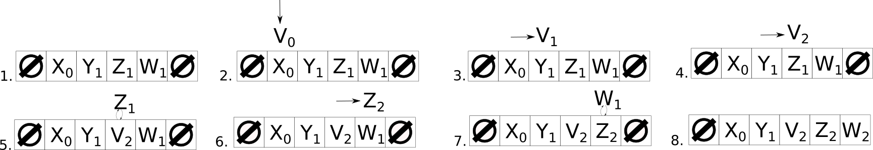
Figure 1. An example Robin Hood insertion where V is inserted into X’s bucket. Each step of the insertion is numbered.

Robin Hood solves this inequality during insertion by moving existing entries around the table. In other words, when the item being relocated has a larger DFB than the item currently being examined, these items are swapped, and the search continues for an empty bucket. Once an empty bucket is found, the relocated item is inserted, and the process terminates. Figure 1 shows an example Robin Hood insertion. In all examples the subscripts represent the DFB of each entry. Step 1 shows the table initially containing X, Y, Z, and W, each with a DFB of 0, 1, 1, and 1 respectively. Step 2 shows that V is to be inserted where X currently resides. Step 3 shows how V doesn’t kick out X, as they’re equal in DFB; the same is true for Y in step 4. Step 5 shows the swap between V and Z, as V is now further away than Z (DFB of 2, compared to 1). Z linear probes further down the table in step 6, and in step 7 swaps with W. Finally, in step 8 W lands in the empty bucket at the end, and the insertion process finishes. In summary, V is swapped with Z, Z is swapped with W, and, finally, W is placed in the empty bucket at the end. Figure 2 shows a comparison of the Robin Hood insertion and the same insertion using the Linear Probing collision resolution. As can be seen, the entry V ends up far further away using Linear Probing than using Robin Hood.

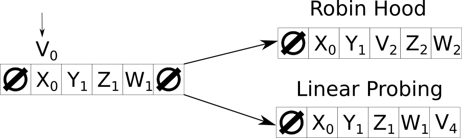
Figure 2. Comparison of Robin Hood to Linear Probing for insertion of V.

The outcome of this shuffling is a reduced average variance in DFB (i.e. reduced probe lengths). Not only does reduced variance make for more predictable and uniform performance, it also allows searches to be culled early, without having to find an empty bucket, which is typically the requirement for calling off a linear probing search. As soon as the item being examined during the search has a lower DFB than the current probing DFB the search can be called off, with the knowledge that it will be unsuccessful: the item being searched for cannot possibly be present in the table, as it would already have kicked out any items with a lower DFB than itself. Figure 3 shows an example Robin Hood search operation. The key U is being queried, probing the table as far as the bucket containing Z before terminating. The linear probing is shown in steps 1 to 3, while termination happens at step 4. Termination is possible as U is 3 buckets away from its original bucket, whereas Z is only 2, meaning U can’t possibly be in the table. The reasoning is that if U was being inserted it would have displaced Z for having a higher DFB than itself; therefore, it cannot possibly be in the table. A similar search taking place using linear probing would have to keep searching until an empty bucket is found, resulting in far more probes at higher load factors, and higher amounts of cache misses too. We refer to this search mechanism as the Robin Hood invariant. Violating this invariant leads to a corrupted table, potentially losing items in the table. These factors enable Robin Hood to support a higher load factor, given that the expected search is only 2.6 probe counts on average for successful searches, and $\mathcal{O}(ln(n))$ for unsuccessful searches [7].

Figure 3. Example Robin Hood search, querying the table for the entry U.

Deletion in Robin Hood is more complicated than in linear probing. In linear probing one can simply tombstone a bucket, as it does not matter what entry was there before. However, in Robin Hood the DFB of the entry matters, as subsequent searches employ this metric to determine if the entry being queried is contained in the table. The solution to this is to either logically mark the entry as deleted, or shift back every entry in front of it until some criterion is met. Logical deletion is unacceptable, as it causes the table to fill up and lose its efficiency, resulting in unnecessary resizes. Backward shifting effectively undoes the insertion of the entry we wish to delete from the table. An example of this is given in Figure 4. Since the removing thread cannot tell which entries the item to be deleted originally displaced to get there (assuming they aren’t at their ideal bucket), we must shift back all items. The shifting is continued until we find an empty bucket or an item in its ideal bucket. Step 1 shows the initial table, step 2 shows the “nulling” of Y. Steps 3, 4, and 5 show a backward shifting of entries within the table. Step 6 shows the termination of the shifting, as an empty bucket is ahead of W.

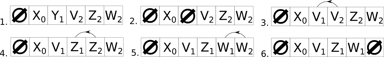
Figure 4. Example Robin Hood deletion. Entry in question is Y.

2.3. K-CAS

K-CAS or, multi-word-compare-and-swap, is an extended version of CAS, supporting multiple compare-and-swap operations on many distinct memory locations, all of which either succeed or else fail together. Our algorithm employs a modified version of the K-CAS originally proposed by Harris, Kaiser and Pratt [17]. The K-CAS algorithm does come at a small cost, reserving an additional 0-2 bits for each word being manipulated by the algorithm. These reserved bits are needed to store run-time type information that allows descriptors to be distinguished from normal values. The standard K-CAS interface provides two functions for basic reading and writing, K_CAS_READ(loc: T*) -> T and K_CAS_WRITE(loc: T*, T val) -> void, and a mechanism for adding addresses and their values to a descriptor. The rationale for needing dedicated read and write functions is that the values being operated on have specific bits reserved to indicate an ongoing K-CAS operation. Both the read and write functions help any pending K-CAS operation installed at that particular memory location.

Traditional K-CAS implementations require a memory reclaimer system, as each descriptor must be fresh to avoid the ABA problem [29] . However, the specific K-CAS implementation we use, developed by Arbel-Raviv and Brown [4], employs descriptor reuse, thereby eliminating the need for a freshly allocated descriptor for each operation. Given that this implementation does not require a memory allocation per K-CAS operation, or a reclaimer, its performance is substantially improved. This enhancement makes K-CAS a feasible concurrency primitive and, as we show, allows it to outperform the best lock-based hash table algorithms.

3. Algorithm

3.1. Challenges For Concurrent Robin Hood

The primary challenge in making Robin Hood concurrent is, unsurprisingly, the modifying operations on the table. Both Add and Remove can modify large parts of the table, with Add potentially performing a global table reorganisation, and Remove potentially shifting back many entries. These problems defeat naive solutions such as sharded locks, as Add could potentially grab all of them, leading to no concurrency. Another issue is that of deadlock; insertions at two different points in the table might grab the locks in a cyclic manner, leading to deadlock. For example, the table could have 8 locks with 8 ongoing insertions in 8 different locations. Initially, each insertion will grab one lock corresponding to the original location. If all insertions relocate an entry to another lock section, deadlock occurs. To achieve a truly concurrent implementation of Robin Hood we need an efficient mechanism to update large disparate parts of the underlying table. For this there are two options. The first is K-CAS, which became feasible from a performance standpoint thanks to the work of Arbel-Raviv and Brown [4]. The second choice is hardware transactional memory, which we use to provide efficient speculative lock-elision [31].

3.2. Overview

K-CAS is a natural choice for relocation-based hash table algorithms. It prohibits a number of issues that typical concurrent algorithms run into, for example, examining whether invariants hold during some intermediate operation or state. K-CAS behaves like an expressively weaker transactional memory [19], but unlike hardware transactional memory [37], it has well defined progress guarantees. Another reason for using K-CAS is that keys can be stored directly in the table, thus improving cache locality. The entry relocations initiated by modifications are summarised into a K-CAS descriptor instead of relying on in-place modifications of the table featuring entry relocation information. Threads cannot see a K-CAS operation partially completed. Nevertheless, special considerations need to be made for operations when reading the table, as they can experience inconsistent views if applied naively.

Since entries can be moved around during concurrent reads, they could inadvertently miss a key due to some ongoing relocation operation. For example, when Contains uses the Robin Hood invariant to terminate a search early, there is a race with a concurrent Remove which could have shifted that particular entry in question back through the table, behind the reader, leading to an incorrect result. This happens when Remove is called on an unrelated entry located in the vicinity of the entry being queried. An example of this phenomenon is illustrated in Figure 5. Here the entry V is being queried while at the same time entry Y is being removed. When the reader gets to the bucket containing V, the remover executes its K-CAS operation, shifting a number of entries, including V, backwards. The searcher then checks the bucket after the shift and sees Z, terminates the search, and falsely declares V as not present in the table.

Figure 5. The problem of concurrent searches and removals. The searcher is trying to find V while entry Y is being removed

Our solution to avoiding this race is to associate each part of the table with a timestamp, updated upon every relocation. Figure 6 shows the correspondence of timestamps to physical buckets in the table. A timestamp can be mapped onto several buckets in the table. The mapping of the timestamps is identical to how locks are sharded in blocking hash tables like Hopscotch Hashing [21]. When a reader is checking for the presence of a particular key, the reader remembers the timestamps encountered during its search. If the key is found and read atomically, then the search can finish. However, if they key isn’t found the reader must check the values of those timestamps after the search has completed. If a discrepancy is found, the search is restarted, otherwise we know for certain the key isn’t in the table. When Remove is executing, it increments the timestamp every time it shifts an entry, and similarly for the Add method.

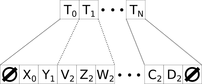
Figure 6. An illustration of how the timestamps are sharded across multiple entries.

3.3. Algorithm Methods

We now outline our algorithm with annotations of code presented in Figures 7, 8, and 9, which highlight and explain important parts and what they do. The algorithmic code has been simplified in two areas. The first simplification involves timestamps: the code provided doesn’t check if a timestamp has already been added to the list, nor does it check the number of entries per timestamp. The second simplification involves Remove when shuffling elements back. In both cases the code is long but simple, so we have excluded it for the sake of clarity.

• 
  fn Contains(key: K) -> bool {
    start_bucket: u64 = hash(key) % size;
  retry:
    timestamps: List<u64> = [];
    for(i = start_bucket, cur_dist = 0;; cur_dist++, i++) {
      i %= size;
      // Add the timestamp for that specific index.
      timestamps.append(read_timestamp(i));
      cur_key: K = K_CAS_load(&table[i]);
      if(cur_key == Nil) { goto timestamp_check; }
      if(cur_key == key) { return true; }
      distance: u64 = calc_dist(cur_key, i); // Robin Hood Invariant
      if (distance < cur_dist) { goto timestamp_check; }
    }
  timestamp_check:
    // Compare every timestamp.
    for(i = start_bucket, idx = 0; idx < timestamps.size(); i++, idx++) {
      i %= size;
      if(list[idx] != read_timestamp(i)) { goto retry; }
    }
    return false; // No key
  }
  

Figure 7. Pseudo-code for Contains

A - Contains

All line numbers refer to Figure 7. At the beginning of the Contains method, a timestamp list is created. Line 8 adds the timestamp for that bucket to the list of timestamps. Line 9 loads a candidate key from the table; if it’s a Nil key, then the search is culled and the timestamps are checked. Line 11 handles a matching key, returning true. Lines 12 - 13 handle the case where the distance of the key is too far away from its original bucket to be present in the table. Lines 17 - 19 check if the timestamp for the particular key has changed since the beginning of the operation, requiring the entire Contains method to be retried, as a key could have been missed.

• 
  fn Add(key: K) -> bool {
    start_bucket: u64 =  hash(key) % size;
  retry:
    active_key: K = key;
    descriptor: K_CAS_Desc = create_descriptor();
    for(i = start_bucket, active_dist = 0;; i++, active_dist++) {
      i %= size;
      cur_timestamp = read_timestamp(i);
      cur_key: K = K_CAS_load(&table[i]);
      if(cur_key == Nil) {
        descriptor.add(&table[i], Nil, active_key);
        res: bool = K_CAS(descriptor); // Attempt to K-CAS operations
        if(!res) { goto retry; }
        return true;
      }
      if(cur_key == key) { return false; }
      distance: u64 = calc_dist(cur_key, i); // Robin Hood Invariant
      if (distance < active_dist) {
        descriptor.add(&table[i], cur_key, active_key); // Swap keys
        // Increment the timestamp within the descriptor.
        add_timestamp_increment(i, cur_timestamp);
        // Swap active key and kick this key down the table
        active_key = cur_key;
        active_dist = distance;
      }
    }
  }
  

Figure 8. Pseudo-code for Add

B - Add

All line numbers refer to Figure 8. Add is quite similar to the serial version. Lines 4 - 5 keep track of the entry currently being relocated via the active key, initially setting the variable to the key being inserted. Add also keeps track of the last timestamp bucket it has incremented. This is hidden behind a helper function called add_timestamp_increment. Timestamps are incremented to prevent a concurrently running Add or Remove from interfering with the correctness of the method. Lines 10 - 14 attempt to insert the key currently being relocated into a Nil bucket, retrying the whole Add operation on failure. Line 16 returns false upon a key match, as the entry is already in the set. Lines 17 - 24 check if an entry needs to be relocated, replacing it with the entry currently being relocated in the thread’s K-CAS descriptor.

• 
  fn Remove(key: K) -> bool {
    start_bucket: u64 = hash(key) % size;
  retry:
    timestamps: List<u64> = [];
    descriptor: K_CAS_Desc = create_descriptor();
    for(i = start_bucket, cur_dist = 0;; cur_dist++, i++) {
      i %= size;
      // Add the timestamp for that specific index.
      timestamps.append(read_timestamp(i));
      cur_key: K = K_CAS_load(&table[i]);
      if(cur_key == Nil) { goto timestamp_check; }
      if(cur_key == key) {
        // Shuffle items down until a Nil key or dist(key) == 0
        shuffle_items(i, cur_key);
        res: bool = K_CAS(descriptor);
        if(!res) { goto retry; }
        return true;
      }
      distance: u64 = calc_dist(cur_key, i); // Robin Hood Invariant
      if (distance < cur_dist) { goto timestamp_check; }
    }
  timestamp_check:
    // Compare every timestamp.
    for(i = start_bucket, idx = 0; idx < timestamps.size(); i++, idx++) {
      i %= size;
      if(list[idx] != read_timestamp(i)) { goto retry; }
    }
    return false;
  }
  

Figure 9. Pseudo-code for Remove

C - Remove

All line numbers refer to Figure 9. Remove is a combination of Contains and Add. First, Remove tries to find the key. If the key isn’t found then, as per Contains, timestamps are checked in case a concurrent Remove or Add has relocated the key during its search. If a key is found, then the process of deletion begins. Lines 12 - 17 constitute the deletion process. The function shuffle_items linearly shuffles items back until a Nil key is found, or else an entry with a DFB of 0 is found. As mentioned earlier, the function is simple, though expansive, so we exclude it. Each linear shuffle is put into the K-CAS descriptor, with line 15 performing the K-CAS operation. The ultimate outcome of this operation is the physical deletion of the entry. Lines 19 - 20 check for the Robin Hood invariant, terminating the search and checking timestamps if the criterion is met. Like Contains, Remove will restart if there is a discrepancy in the timestamps. Lines 24 - 26 check the timestamps of each bucket read.

3.4. Proof Of Correctness

The proof of correctness is relatively simple and informal. K-CAS [17] is itself linearisable [22], and K-CAS encodes all relocations and timestamp increments to the data structure in its descriptors. An invocation of K-CAS essentially turns each modification operation on the table into a transaction. Every Add or Remove call that results in relocations increments a timestamp via the K-CAS operation; if any reading thread was to examine the table’s contents during a relocation, the reader could compare before and after timestamps so as to ensure that no entry was moved during the search. Furthermore, because each reader also helps the K-CAS operation, reading the timestamp will result in one of three outcomes. Either the reader will read a new timestamp value, the same timestamp, or else help the operation complete an ongoing K-CAS operation by reading the new timestamp if the operation succeeds or the old one if it fails. Readers need only ensure that the timestamps haven’t changed since their initial reading. Since Remove can exit in two ways, it has two different linearisation points. The linearisation point of Add, and the first code path of Remove are at line 12 in Figure 8 and line 15 in Figure 9, where the K-CAS is successfully called. Contains and the second exit point of Remove linearise at the point of reading their last timestamp from their search on lines 8 and 9 respectively.

3.5. Progress

The progress of each operation is parameterised by the progress of the K-CAS operation. If the K-CAS operation is blocking, then all method calls on the hash table are blocking. However if we have a lock-free implementation of K-CAS, then the following classifications for each method occur. Calls to Contains are obstruction-free [18], as other concurrent operations can cause a relevant timestamp to change, thus forcing the method to restart. Threads calling Contains can starve but they are not blocked if another thread dies. Add has the same progress guarantees as Contains and for the same reasons, other modifying operations can modify relevant timestamps forcing the method to fail and restart. Timestamps are not guaranteed to correspond to the entries the method wants to examine, they are coarse and each timestamp corresponds to a number of entries. Remove must first find the entry it wishes to remove, effectively running the same code as Contains and thus having the same classification. Afterwards, once found, the deletion and subsequent shuffling of that entry is also obstruction-free since other irrelevant operations with the same timestamp can interfere with its progress. In summary, lock-free K-CAS calls to Contains, Add, and Remove are obstruction-free.

4. Performance, Results, and Discussion

In this section we detail the performance and implementation of our algorithms. All of our code is made freely available online [23]. This includes K-CAS Robin Hood, the hardware transactional [19] variant of Robin Hood Hashing with lock-elision [31], the implementation of alternative competing algorithms (either coded by us or obtained via online sources), and benchmarking code which allows readers to replicate our results.

4.1. Experimental Setup

For our experiments we opted to use a set of microbenchmarks which stressed the hash table under various capacities and workloads. Our benchmarks were run on a 4 CPU machine, with each CPU (Intel® Xeon® CPU E7-8890 v3) featuring 18 cores with 36 hardware threads and 512 GiB RAM. The machine was running Ubuntu 14.04 with kernel version 3.13.0-141. Each thread was pinned to a specific core during testing. When scaling the number of threads, care was taken to pin the thread to a new core, avoiding HyperThreading™ until necessary. Once all non HyperThreading™ cores on each CPU were exhausted, HyperThreading™ was employed thereafter. The rational for this scheduling choice is that algorithms which employ hardware transactional memory are disproportionately penalised by HyperThreading™ and some mainstream operating systems, such as OpenBSD, disable HyperThreading™. As a result we shed light on how our algorithms would scale on those systems. NUMA memory effects were controlled by specifying where each thread could allocate using the numactl command, allocating on the RAM banks closest to the running CPUs as they came into use.

The algorithms used in the experiments are as follows: K-CAS Robin Hood, Transactional Lock-Elision Robin Hood Hashing, Hopscotch Hashing [21], a Lock-Free Linear Probing hash table described by Nielsen and Karlsson [27], and Michael’s lock-free hash table [25].

A number of workload configurations were used in graphing the results. Four load factors of 20%, 40%, 60%, and 80% were chosen, along with two update workload configurations, namely 10% and 20%, referred to herein as “light” and “heavy”. Both of the workload configurations were tried at the specified load factors, and both were used for comparing the different Robin Hood Hashing algorithms against each other, and against competitors. We sized the tables at $2^{23}$ to ensure that they wouldn’t fit into the cache, thereby exposing each algorithm’s effective cache use. The key space was equal to the size of the table, and was filled to the specified load factors. The scalable JeMalloc [12] allocator was used in the experiments and no memory reclamation system was used in algorithms that traditionally require one.

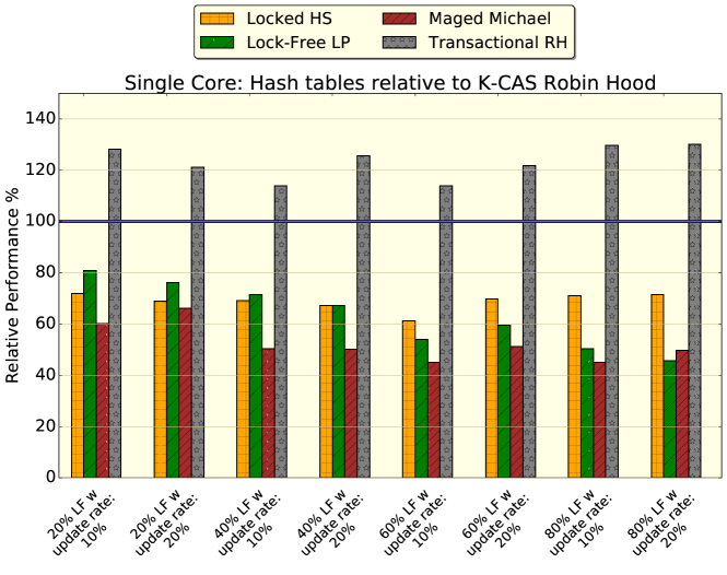
Figure 10. Single-core performance of the hash tables relative to K-CAS Robin Hood.

The testing process was carried out as follows: Each thread calls a random method with a random argument from some predefined method and key distribution. All threads are synchronised before execution on the data structure, and for a specified amount of time rather than a specific number of iterations. Each thread counts the number of operations it performed on the structure during the benchmark. The total amount of operations per microsecond for all threads is then graphed. Each experiment was run five times for 10 seconds each, and the average of each result was computed and plotted. All of our algorithms were written in C++11, and compiled with g++ 4.8.4 with O3 level of optimisation. Cache misses were collected via PAPI [36].

4.2. Discussion and results

In order to gain an understanding of general operation overhead, we measured single-core performance. The performance is measured against K-CAS Robin Hood. In Figure 10 we see that Hopscotch Hashing, Maged Michael’s Separate Chaining, and Lock-Free Linear Probing are significantly slower than the other algorithms. The reason for this is two-fold. First, the issue of cache efficiency arises: Lock-Free Linear Probing and separate chaining use dynamic memory allocation, meaning that a pointer dereference is needed for every bucket access. While Hopscotch Hashing does not use dynamically allocated memory, it does put more pressure on the cache by storing the original hash of a key inside the table. However it should be noted that it doesn’t put as much pressure on the cache as K-CAS Robin Hood, as per Table 1. The second issue is the amount of work carried out for every operation: Hopscotch Hashing is the most complicated, executing more code and performing more operations. Transactional Robin Hood has higher performance than K-CAS Robin Hood as it does not require to consult the K-CAS descriptor and timestamps.

	Configurations (Load factor w/ Updates)
Hash Tables	20% w/ 10%	20% w/ 20%	40% w/ 10%	40% w/ 20%	60% w/ 10%	60% w/ 20%	80% w/ 10%	80% w/ 20%
Hopscotch Hashing	88%	82%	70%	71%	64%	68%	59%	65%
Lock-Free LP	185%	207%	227%	240%	294%	305%	430%	453%
Maged Michael	109%	105%	95%	95%	89%	93%	85%	91%
Transactional RH	86%	85%	82%	78%	89%	86%	93%	90%

Table 1. Cache misses relative to K-CAS Robin Hood single-core.

The cache results can be seen in Table 1 as a percentage relative to K-CAS Robin Hood for a single-core. These cache statistics were measured over the course of the entire execution of the benchmark for each table and for each configuration. Hopscotch Hashing fairs very well as it is able to skip over irrelevant entries. Lock-Free Linear Probing uses dynamic memory and thus puts enormous pressure on the cache. Another downside is as the table fills up over time with tombstones, it forces operations to take roughly the same amount of time regardless of load factor. This phenomenon is called contamination [15]. Maged Michael [25] fairs reasonably well even though it uses dynamic memory. Very few buckets have more than a single node meaning few extra nodes are needed. Transactional Lock-Elision Robin Hood performs better as it does not need to consult an extra timestamp array or any extra K-CAS descriptor, which would require an extra level of indirection.

As is clear from the multi-core results in Figure 11, 12 the K-CAS Robin Hood Hashing algorithm either scales better than or is competitive with its opposition. Across all graphs there are two significant dips in performance. The first is at 18 threads, where threads are pinned to a different CPU socket. The use of another socket requires inter-socket communication and NUMA effects, reducing overall performance. The second is when increasing from 72 to 81 threads, which is the point where HyperThreading™ kicks in. This kink is particularly pronounced for the transactional Robin Hood variant, which never recovers after that point. Both of these effects become most pronounced when a significant write load is placed on the tables.

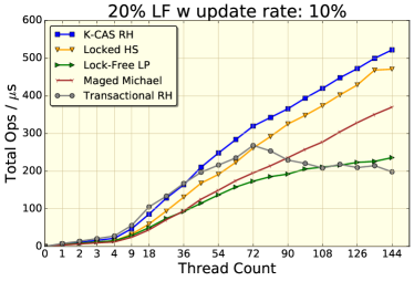
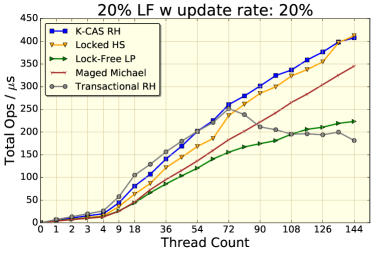
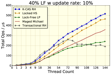
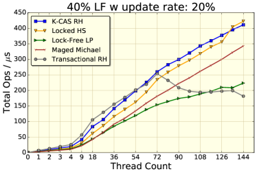
Figure 11. Cumulative operations per microsecond for the hash tables at 20% and 40% load factors at two update rates. (Higher is better)

Each of the workloads highlights the particular performance characteristics of each hash table. The update-light (10% writes) workload shows K-CAS Robin Hood dominating the competition across all thread counts and load factors. The update-heavy (20% writes) workload has two distinct outcomes predicated on the table load factor. The lower load factor shows K-CAS Robin Hood is slightly beaten out by the Transactional Robin Hood variant until the 72 thread mark, wherein it drops off entirely. K-CAS Robin Hood also edges out Hopscotch Hashing throughout most of the update-heavy workload until the very upper end of the thread count, where it is slightly outclassed. However, at higher load factors K-CAS Robin Hood demonstrates similar relative performance to the lower load factor benchmarks but maintains its lead over Hopscotch Hashing. All workloads show the gap between K-CAS Robin Hood and Hopscotch begins to narrow once HyperThreading™ kicks in. As mentioned earlier, in every configuration the transactional variant of Robin Hood scales very well until 72 threads, after which HyperThreading™ causes a huge kink in performance, and the algorithm never recovers. Maged Michael scales well in the tested workloads, however the gradient of the line isn’t steep enough to challenge K-CAS Robin Hood or Hopscotch Hashing. Lock-Free Linear Probing does the worst of all, ending up at the same end point as Transactional Robin Hood.

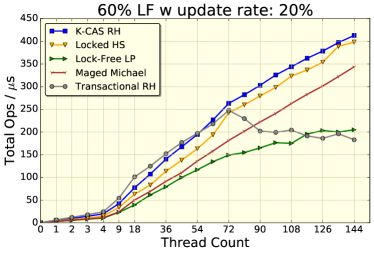
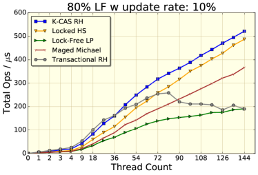
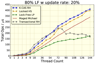
Figure 12. Cumulative operations per microsecond the hash tables at 60% and 80% load factors at two update rates. (Higher is better)

4.3. Future Work

An issue we don’t deal with is resize, specifically, when to resize the table and how to do it. Lock-free resize methods have been discussed in the literature ([8], [32]). To the best of our knowledge there has not yet been a formally published generic hash table resize method. Another item for future work is a combination of lock-free K-CAS and transactional [19] memory, such as the algorithm presented by Trevor Brown [6] for lock-free trees. A similar exploration for Robin Hood and other the hash tables benchmarked would be of interest. Work done by Siakavaras et el. [33] shows that naive application of hardware transactional systems to data-structures typically perform poorly and require algorithm modifications to operate efficiently. Future work aimed at determining the optimal modifications for Robin Hood might elevate its performance for hardware transactional memory.

5. Conclusion

We have presented an obstruction-free Robin Hood Hashing algorithm which achieves superior performance relative to other concurrent algorithms with similar capabilities, and a hardware transaction variant which demonstrates best in class performance. These results establish that the Robin Hood algorithm is algorithmically suited to concurrency. Our experiments have shown that it scales strongly at all thread counts. Unlike linear probing, the algorithm can scale effectively to significantly higher load factors. It is very simple in nature, relying primarily on an efficient K-CAS, as well as being highly portable, using only single word compare-and-swap instructions, with no memory reclaimer required. Our results improve upon the state of the art in the field which is more than 10 years old.

References

- [1] D. Alistarh, W. Leiserson, A. Matveev, and N. Shavit. Threadscan: Automatic and scalable memory reclamation. In SPAA, 2015.
- [2] D. Alistarh, W. Leiserson, A. Matveev, and N. Shavit. Forkscan: Conservative memory reclamation for modern operating systems. In EuroSys, 2017.
- [3] A. Amighi, S. Blom, and M. Huisman. Vercors: A layered approach to practical verification of concurrent software. In 24th Euromicro International Conference on Parallel, Distributed, and Network-Based Processing, PDP, 2016.
- [4] M. Arbel-Raviv and T. Brown. Reuse, don’t recycle: Transforming lock-free algorithms that throw away descriptors. In DISC, 2017.
- [5] M. Batty. The c11 and c++11 concurrency model. http://www.cl.cam.ac.uk/~mjb220/thesis/thesis.pdf. Accessed: 2017-05-04.
- [6] T. Brown. A template for implementing fast lock-free trees using htm. In PODC, 2017.
- [7] P. Celis. Robin Hood Hashing. PhD thesis, University of Waterloo, Waterloo, Ont., Canada, Canada, 1986.
- [8] C. Click. Lock-free/wait-free hash table. http://web.stanford.edu/class/ee380/Abstracts/070221_LockFreeHash.pdf. Accessed: 2017-05-04.
- [9] N. Cohen and E. Petrank. Efficient memory management for lock-free data structures with optimistic access. In Proceedings of the 27th ACM symposium on Parallelism in Algorithms and Architectures, pages 254–263. ACM, 2015.
- [10] T. Cormen, C. Stein, R. Rivest, and C. Leiserson. Introduction to Algorithms. McGraw-Hill Higher Education, 2nd edition, 2001.
- [11] U. Drepper. What Every Programmer Should Know About Memory, 2007.
- [12] J. Evans. Jemalloc, Retrieved 2018-08-06. Available at https://github.com/jemalloc/jemalloc.
- [13] S. Feldman, P. LaBorde, and D. Dechev. A wait-free multi-word compare-and-swap operation. International Journal of Parallel Programming, 43(4):572–596, Aug 2015.
- [14] K. Fraser. Practical lock-freedom. Technical report, University of Cambridge, Computer Laboratory, 2004.
- [15] G. Gonnet and R. Baeza-Yates. Handbook of Algorithms and Data Structures: In Pascal and C (2Nd Ed.). Addison-Wesley Longman Publishing Co., Inc., Boston, MA, USA, 1991.
- [16] T. Harris. A pragmatic implementation of non-blocking linked-lists. In Proceedings of the 15th International Conference on Distributed Computing, DISC, 2001.
- [17] T. Harris, K. Fraser, and I. Pratt. A practical multi-word compare-and-swap operation. In Proceedings of the 16th International Conference on Distributed Computing, DISC ’02, pages 265–279, London, UK, UK, 2002. Springer-Verlag.
- [18] M. Herlihy, V. Luchangco, and M. Moir. Obstruction-free synchronization: Double-ended queues as an example. In Proceedings of the 23rd International Conference on Distributed Computing Systems, ICDCS ’03. IEEE Computer Society, 2003.
- [19] M. Herlihy and J. Moss. Transactional memory: Architectural support for lock-free data structures. In Proceedings of the 20th Annual International Symposium on Computer Architecture, ISCA ’93. ACM, 1993.
- [20] M. Herlihy and N. Shavit. The Art of Multiprocessor Programming. Morgan Kaufmann, 1 edition, March 2008.
- [21] M. Herlihy, N. Shavit, and M. Tzafrir. Hopscotch Hashing. In DISC ’08: Proceedings of the 22nd international symposium on Distributed Computing, pages 350–364, Berlin, Heidelberg, 2008. Springer-Verlag. doi:10.1007/978-3-540-87779-0\_24.
- [22] M. Herlihy and J. Wing. Linearizability: A correctness condition for concurrent objects. ACM Trans. Program. Lang. Syst., 12(3):463–492, July 1990.
- [23] R. Kelly. Source code for lock-free robin hood benchmark. https://github.com/DaKellyFella/concurrent-robin-hood-hashing. Accessed: 2018-11-14.
- [24] K. Rustan M. Leino and Peter Müller. A Basis for Verifying Multi-threaded Programs, pages 378–393. Springer Berlin Heidelberg, Berlin, Heidelberg, 2009.
- [25] M. Michael. High performance dynamic lock-free hash tables and list-based sets. In Proceedings of the fourteenth annual ACM symposium on Parallel algorithms and architectures, SPAA. ACM, 2002.
- [26] M. Michael. Hazard pointers: Safe memory reclamation for lock-free objects. IEEE Trans. Parallel Distrib. Syst., 15(6):491–504, June 2004.
- [27] J. Nielsen and S. Karlsson. A scalable lock-free hash table with open addressing. SIGPLAN Not., 51(8):33:1–33:2, February 2016.
- [28] D. Lea P. William, S. Adve. Jsr 133: Javatm memory model and thread specification revision. https://www.jcp.org/en/jsr/detail?id=133. Accessed: 2017-05-04.
- [29] A. Padegs. System/370 extended architecture: Design considerations. IBM Journal of Research and Development, 27(3):198–205, 1983.
- [30] C. Purcell and T. Harris. Non-blocking Hashtables with Open Addressing, pages 108–121. Springer Berlin Heidelberg, Berlin, Heidelberg, 2005.
- [31] R. Rajwar and J. Goodman. Speculative lock elision: Enabling highly concurrent multithreaded execution. In Proceedings of the 34th annual ACM/IEEE international symposium on Microarchitecture, pages 294–305. IEEE Computer Society, 2001.
- [32] O. Shalev and N. Shavit. Split-Ordered Lists: Lock-Free Extensible Hash Tables. In Proceedings of the 22nd Annual ACM Symposium on Principles of Distributed Computing (PODC), 2003.
- [33] D. Siakavaras, K. Nikas, G. Goumas, and N. Koziris. Massively concurrent red-black trees with hardware transactional memory. In 2016 24th Euromicro International Conference on Parallel, Distributed, and Network-Based Processing (PDP), 2016.
- [34] H. Sutter. The Free Lunch Is Over: A Fundamental Turn Toward Concurrency in Software. Dr. Dobb’s Journal, 30(3), 2005.
- [35] Rust Core Team. Rust collections hash table. https://doc.rust-lang.org/std/collections/struct.HashMap.html. Accessed: 2017-05-07.
- [36] D. Terpstra, H. Jagode, H. You, and J. Dongarra. Collecting performance data with papi-c. In Tools for High Performance Computing 2009, pages 157–173, Berlin, Heidelberg, 2010. Springer Berlin Heidelberg.
- [37] R. Yoo, C. Hughes, K. Lai, and R. Rajwar. Performance evaluation of intel; transactional synchronization extensions for high-performance computing. In Proceedings of the International Conference on High Performance Computing, Networking, Storage and Analysis, SC. ACM, 2013.