Blind prediction of protein B-factor and flexibility

Abstract

Debye-Waller factor, a measure of X-ray attenuation, can be experimentally observed in protein X-ray crystallography. Previous theoretical models have made strong inroads in the analysis of B-factors by linearly fitting protein B-factors from experimental data. However, the blind prediction of B-factors for unknown proteins is an unsolved problem. This work integrates machine learning and advanced graph theory, namely, multiscale weighted colored graphs (MWCGs), to blindly predict B-factors of unknown proteins. MWCGs are local features that measure the intrinsic flexibility due to a protein structure. Global features that connect the B-factors of different proteins, e.g., the resolution of X-ray crystallography, are introduced to enable the cross-protein B-factor predictions. Several machine learning approaches, including ensemble methods and deep learning, are considered in the present work. The proposed method is validated with hundreds of thousands of experimental B-factors. Extensive numerical results indicate that the blind B-factor predictions obtained from the present method are more accurate than the least squares fittings using traditional methods.

Keywords: Weighted colored graph, Protein flexibility, Gradient boosted trees, Random forest, Convolutional neural network.

1 Introduction

Protein beta factor (B-factor) or temperature factor (Debye-Waller factor) is a measure of atomic mean squared displacement or uncertainty in the X-ray scattering or neutron scattering structure determination. For a given protein at a given temperature, a large B-factor is caused by the atomic thermal fluctuation and low attenuation rate. The latter depends also on the experimental modality. For example, the hydrogen atom has a low attenuation rate in X-ray scattering because of its small number of electrons but has a normal attenuation rate for neutron scattering. For a given element type under the same experimental condition, the B-factor of an atom is determined by its intrinsic flexibility and possible crystal packing effects. It has been previously shown that intrinsic flexibility correlates to important protein conformational variations [1]. That is, protein structural fluctuation provides an important link between structure, and function of a protein. As such, accurate prediction of protein B-factors is an important and meaningful metric in understanding protein structure, flexibility and function [2].

One successful class of methods in protein B-factor prediction was those that used elastic mass-and-spring networks derived from Hooke’s Law. These models represent the alpha carbons of biological macromolecules as a mass and spring network to predict B-factors based on a harmonic potential. Each alpha carbon in a protein is regarded as a node in the network, and edges are weighted based on a potential function. In these models, a pair of nodes is connected by an edge if they fall within a predefined Euclidean cutoff distance. This approach captures the local non-covalent interactions between an individual alpha carbon atom and nearby alpha carbon atoms.

Normal mode analysis (NMA) was one of the first mass-and-spring methods used for protein B-factor prediction. This method is independent of time and makes use of a Hamiltonian matrix for atomic interactions. Here the modes of the system correspond to motion where all parts of the molecule are moving sinusoidally with the same frequency and phase. Moreover, eigenvalues of the system correspond to characteristic frequencies that correlate with protein B-factors. Low-frequency modes correlate with operative motions which can be useful for hinge detection. NMA has also been found to be useful in characterizing coarse grain deformation of supramolecular complexes. [1, 3, 4, 5]

The elastic network model (ENM) was introduced to reduce the computational cost of NMA by using a simplified spring network [6]. One successful ENM model is the anisotropic network model (ANM). This model uses a simplified spring potential between each residue, then determines the modes of the system via matrix diagonalization. ANM still retains many of the insightful features of NMA but with a much lower computation cost.[7, 8, 9]

The Gaussian network model (GNM) was introduced as a simplified method for B-factor prediction [8]. Similar to previous models, a graph network is constructed using alpha carbon as nodes and edges based on a prescribed cutoff distance. GNM uses a distance-based Kirchhoff (or connectivity) matrix to represent the interaction between each two alpha carbon atoms (nodes). The expectation values of residue fluctuations or mean-square fluctuations are found in the diagonal terms of a covariance matrix. GNM provides good-coarse grained results with relatively low computational cost. [10]

More recently, the flexibility and rigidity index (FRI) methods have provided improved results. These methods construct graph centrality based on radial basis functions which scale distance non-linearly [11]. Fast FRI (fFRI) provides a version of FRI with a very low computation cost while still maintaining satisfactory results [12]. Anisotropic FRI (aFRI) offers a matrix version of FRI to compute protein anisotropic motions. Moreover, the multiscale flexibility rigidity index (mFRI) is able to capture protein multiscale interactions using several radial basis functions with different parameterizations [13, 14].

Previously the authors introduced a multiscale weighted colored graph (MWCG) model for protein flexibility analysis [15]. The MWCG is a geometric graph model that offers the most accurate and reliable protein flexibility analysis and B-factor prediction to date. It is about 40% more accurate than GNM [15]. The basic idea of MWCG is to color (label) a protein graph based on element interaction types. Each atom of given an element type selection represents a graph vertex and subgraphs are defined according to specific heavy element types. A generalized centrality is defined for each subgraph vertex. Using various parameterizations of radial basis functions, this method is able to capture multiscale element specific interactions. The MWCG method can be combined with various earlier FRI approaches, such as fFRI, mFRI and aFRI, to further strengthen its power in the analysis of intrinsic protein flexibility. Additionally, MWCG works well not only for C_α carbons but also for all the atoms in a protein, i.e., non-C_α carbon, nitrogen, oxygen, and sulfur atoms. Hydrogen atoms can be treated similarly if they are available in the dataset [15].

All of the aforementioned methods are designed for the analysis of intrinsic protein flexibility due to protein structure and packing crystal packing. However, none was designed to predict the B-factors of an unknown protein. Indeed, all of these methods fit experimental B-factors of given protein by the least squares algorithm. They generally do a poor job in predicting flexibility across proteins. Stated differently, the fitting coefficients obtained from one protein are not applicable to a different protein in general. This is largely due to the fact that protein B-factor depends also on a large number of effects, including X-ray crystal quality, crystal symmetry (i.e., space group), data collecting method, data collecting environment, equipment condition, etc. Consequently, the blind prediction of protein flexibility and B-factors remains a major challenge.

Recently, advances in graphics processing unit (GPU) computing and optimization have led to impressive biophysical predictions for various problems using machine learning, particularly, deep learning techniques. In this work, we propose machine-learning based methods for blind protein B-factor predictions. We introduce two sets of features, the global ones, and local ones. Global features are designed to represent crystal and experimental conditions across different proteins, while local features are devoted to describing structural and atomic properties within a protein structure. We compile and engineer local and global features from a large set of known protein data as a training set, then apply machine learning techniques to establish regression models which are used for the blind prediction of B-factors of unknown protein structures. In terms of machine learning procedures, we use a variety of local and global protein features of a labeled training set to construct regression models that can blindly predict the B-factors of a test set, consisting of entirely new proteins. In this work, we explore the random forest, boosted gradient decision trees, and deep learning methods for blind protein B-factor predictions. Using a large and diverse set of proteins from the protein data bank ensures technical robustness. In addition to previously explored features such as MWCG kernels and element type, we also include secondary structural information and local packing density features to further improve our results.

2 Methods and algorithms

The success of blind protein B-factor predictions depends crucially on the representation of biomolecular structures. We employ MWCGs as local features to describe protein structures. A brief review of MWCGs is given below.

2.1 Multiscale weighted colored graphs

Graph theory concerns the relationship of a set of vertices, denoted as $V$, in terms of pairwise connectivity, i.e., edges $E$. We use a graph to describe the non-covalent interactions in proteins. To improve our graph theory representation, we consider colored graphs in which different types of elements are labeled. We classify labeled protein atoms into subgraphs where colored edges correspond to element specific interactions. Specifically, we label the $i$th atom by its element type $\alpha_{j}$ and position ${\bf r}_{j}$. As such, vertices are labeled as

$$V=\{(\mathbf{r}_{j},\alpha_{j})|\mathbf{r}_{j}\in{\rm I\!R}^{3};\alpha_{j}\in{\cal C};j=1,2,\ldots,N\}$$

, where ${\cal C}=${C, N, O, S } are the set of elements whose pairwise interactions will be considered. Hydrogen is omitted from this list due to its absence from most PDB data and can be added without affecting the present description. The set of edges in the colored protein graph are element specific pairs ${\cal P}=${CC,CN,CO,CS,NC,NN,NO,NS,OC,ON,OO,OS,SC,SN,SO,SS}. For example, the subset ${\cal P}_{3}=${CO} contains all directed CO pairs in the protein such that the first atom is a carbon and the second one is a nitrogen. The direction is maintained because the edge, $E$, is a set of weighted and directed interaction kernels of various pairs of atoms,

$$E=\{\Phi^{k}(||\mathbf{r}_{i}-\mathbf{r}_{j}||;\eta_{ij})|(\alpha_{i}\alpha_{j})\in{\cal P}_{k};k=1,2,\ldots,10;i,j=1,2,\ldots,N\},$$ (1)

where $||\mathbf{r}_{i}-\mathbf{r}_{j}||$ is the Euclidean distance between the $i^{th}$ and $j^{th}$ atoms, $\eta_{ij}$ is a characteristic distance between the atoms and $(\alpha_{i}\alpha_{j})$ is a directed pair of element types. Here $\Phi^{k}$ is a correlation function and is chosen to have the following properties [12]

$$\Phi^{k}(||\mathbf{r}_{i}-\mathbf{r}_{j}||;\eta_{ij})=1,\mbox{ as }||\mathbf{r}_{i}-\mathbf{r}_{j}||\rightarrow 0\quad\quad(\alpha_{i}\alpha_{j})\in{\cal P}_{k},$$ (2)

$$\Phi^{k}(||\mathbf{r}_{i}-\mathbf{r}_{j}||;\eta_{ij})=0\mbox{ as }||\mathbf{r}_{i}-\mathbf{r}_{j}||\rightarrow\infty,\quad\quad(\alpha_{i}\alpha_{j})\in{\cal P}_{k}.$$ (3)

Our previous work [12] has shown that generalized exponential functions,

$$\Phi^{k}(||\mathbf{r}_{i}-\mathbf{r}_{j}||;\eta_{ij})=e^{-(||\mathbf{r}_{i}-\mathbf{r}_{j}||/\eta_{ij})^{\kappa}},\quad(\alpha_{i}\alpha_{j})\in{\cal P}_{k};\quad\kappa>0,$$ (4)

and generalized Lorentz functions,

$$\Phi^{k}(||\mathbf{r}_{i}-\mathbf{r}_{j}||;\eta_{ij})=\dfrac{1}{1+(||\mathbf{r}_{i}-\mathbf{r}_{j}||/\eta_{ij})^{\nu}},\quad(\alpha_{i}\alpha_{j})\in{\cal P}_{k};\quad\nu>0,$$ (5)

are good choices which satisfy the assumptions.

The centrality metric used in this work is an extension of harmonic centrality to subgraphs with weighted edges defined by the generalized correlation functions

$$\mu^{k}_{i}=\sum_{j=1}^{N}w_{ij}\Phi^{k}(||\mathbf{r}_{i}-\mathbf{r}_{j}||;\eta_{ij}),\quad(\alpha_{i}\alpha_{j})\in{\cal P}_{k},\quad\forall i=1,2,\ldots,N,$$ (6)

where $w_{ij}$ is a weight function related to the element type. The WCG centrality in Eq. (6) describes the atomic specific rigidity which measures the stiffness at the $i^{th}$ atom due to the $k$th set of contact atoms.

To characterize protein multiscale interactions, we use the atomic specific rigidity index from multiscale weighted colored graphs (MWCGs) introduced in our previous work [15]. The atomic rigidity of $i^{th}$ atom at $n^{th}$ scale due to the $k^{th}$ set of interaction atoms is defined as

$$\mu^{k,n}_{i}={\sum_{j=1}^{N}w_{ij}^{n}\Phi^{k}(||\mathbf{r}_{i}-\mathbf{r}_{j}||;\eta_{ij}^{n})},\quad(\alpha_{i}\alpha_{j})\in{\cal P}_{k},$$ (7)

where $\Phi^{k}(||\mathbf{r}_{i}-\mathbf{r}_{j}||;\eta_{ij}^{n})$ is a correlation kernel, $\eta_{ij}^{n}$ a scale parameter, and $w^{n}_{ij}$ is an atomic type dependent parameter. We set $w^{n}_{ij}=1$ in the present work.

While sulfur atoms play an important role in proteins they are so sparse that their kernels have a negligible effect on the current model. Therefore, it is convenient to consider a subset of ${\cal P}$ in practical computations

$${\cal\hat{P}}=\mbox{\big{\{}CC, CN, CO, NC, NN, NO, OC, ON, OO \big{\}}}.$$ (8)

We chose only C, N, and O element types due to their high occurrence frequency and important biological relevance.

2.2 Machine learning features

2.2.1 Global features

Protein Databank (PDB) ⁢.pdb files provide the spatial atomic coordinates and the B-factor of each atom in a protein as well as a variety of other types of observed data that can be used as features. In addition to the use of PDB spatial coordinates, this work makes use of global features provided in PDB files such as R-value, resolution, and number of heavy atoms. R-value and resolution are global measures of the quality of the atomic model obtained from crystallographic data. Another global feature we consider is the overall protein size. To allow the models to distinguish proteins of different sizes we use one hot encoding with the 10 size ranges

$$[500,750,1000,1500,2000,2500,3000,4000,5000,30000],$$

where a protein element feature size will take on 1 if the number of heavy atoms (carbon, nitrogen, or oxygen) in that protein is less than or equal to the corresponding size and zero for the remaining sizes. For example, a protein with 1700 heavy elements would have the feature size vector for all of its atoms given by

$$[0,0,0,0,1,0,0,0,0,0],$$

.

A frequency distribution of the size categories is provided in Figure 1. There are a total of 12 global protein size features.

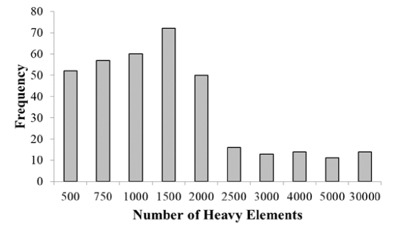
Figure 1: Frequency of the number of heavy elements within the proteins from the 364 protein dataset.

2.2.2 Local features

PDB files also contain amino acid information for each element. Using one hot encoding we include amino acid information for each heavy element which results in 20 amino acid features. Similarly we one hot code the 4 different heavy element types carbon, nitrogen, oxygen, and sulfur for each element resulting in 4 additional features.

We use MWCG rigidity index described in Section 2.1 to create feature vectors for carbon, nitrogen, and oxygen interactions with each element. Moreover, to capture multiscale interactions we use 3 different kernel choices for each interaction type. This results in a total of 9 MWCG feature vectors. The parametrization of the kernels is chosen based on our previous work and is provided in Table 1.[15]

Kernel Type	$\kappa$	$\eta^{n}$	$\nu$
Lorentz ($n=1$)	-	16	3
Lorentz ($n=2$)	-	2	1
Exponential ($n=3$)	1	31	-

Table 1: Parameters used for correlation kernels in a parameter-free MWCG based on previous results.[15]

The MWCG rigidity kernels do not entirely capture the density of nearby atoms. In this work, we define short, medium and long packing density features for each heavy atom. The packing density of the $i^{th}$ atom is defined as

$$p_{i}^{d}=\dfrac{N_{d}}{N},$$

where $d$ is the given cutoff in angstroms, $N_{d}$ is the number of atoms within the Euclidean distance of the cutoff to the $i^{th}$ atom, and $N$ the total number of heavy atoms of the protein. The packing density cutoffs used in this work are provided in Table 2.

Short	Medium	Long
$d<3$	$3\leq d<5$	$5\leq d$

Table 2: Packing density parameters in distance ($d$ Å).

We include secondary structural information generated using the STRIDE software. The STRIDE software provides secondary structural information about a protein given its atomic coordinates as a PDB file. STRIDE designates each atom as belonging to a helix (alpha helix, 3-10 helix, PI-helix), extended conformation, isolated bridge, turn, or coil. Additionally, STRIDE provides $\phi$ and $\psi$ angles and residue solvent accessible area [16]. Taken together this provides 12 secondary features.

2.2.3 MWCG inputs

Using the MWCG method, we apply Lorentz and exponential radial basis functions to construct multi-scale images for each element of a protein. To capture a large variety of scales we construct multiscale kernels for each heavy atom of a protein using various values of $\kappa$, $\nu$, and $\eta$. In particular we use

$$\eta=\{1,2,3,4,5,10,15,20\}$$

and

$$\kappa,\ \nu=\{2,2.5,3,3.5,4,4.5,5,5.5,6,6.5,7,8,9,10,11\}.$$

This results in 2D MWCG images of dimension $(8,30)$. We create images for all carbon, nitrogen, and oxygen interactions for each heavy atom giving each image three channels.

The image matrix is given by $F_{i}^{k}$ in equation 9, where each atom $f_{i}^{k}(l,m,n)$ represents the flexibility index of the $i^{th}$ atom, and $k^{th}$ atom interaction (C, N, or O), $l=\eta$, $m=\{\kappa,\ \nu\}$, and $n$ the type of radial basis function. Values of $n=1$ and $n=2$ correspond to exponential and Lorentz radial basis functions respectively.

$$\left.F_{i}^{k}=\begin{bmatrix}f_{i}^{k}(1,2,1)&f_{i}^{k}(1,2.5,1)&\ldots&f_{i}^{k}(1,11,1)&f_{i}^{k}(1,2,2)&f_{i}^{k}(1,2.5,2)&\ldots&f_{i}^{k}(1,11,2)\\ f_{i}^{k}(2,2,1)&f_{i}^{k}(2,2.5,1)&\ldots&f_{i}^{k}(2,11,1)&f_{i}^{k}(2,2,2)&f_{i}^{k}(2,2.5,2)&\ldots&f_{i}^{k}(2,11,2)\\ \vdots&&&&&&\vdots\\ f_{i}^{k}(15,2,1)&f_{i}^{k}(15,2.5,1)&\ldots&f_{i}^{k}(15,11,1)&f_{i}^{k}(15,2,2)&f_{i}^{k}(15,2.5,2)&\ldots&f_{i}^{k}(15,11,2)\\ \makebox[0.0pt][l]{$\smash{\underbrace{\phantom{\begin{matrix}f_{i}^{k}(20,2,1)&f_{i}^{k}(20,2.5,1)&\ldots&f_{i}^{k}(20,11,1)\end{matrix}}}_{\text{$\kappa$}}}$}f_{i}^{k}(20,2,1)&f_{i}^{k}(20,2.5,1)&\ldots&f_{i}^{k}(20,11,1)&\makebox[0.0pt][l]{$\smash{\underbrace{\phantom{\begin{matrix}f_{i}^{k}(20,2,2)&f_{i}^{k}(20,2.5,2)&\ldots&f_{i}^{k}(20,11,2)\end{matrix}}}_{\text{$\nu$}}}$}f_{i}^{k}(20,2,2)&f_{i}^{k}(20,2.5,2)&\ldots&f_{i}^{k}(20,11,2)\\ \end{bmatrix}\right\}\eta$$ (9)

2.3 Machine learning algorithms

A grid search was implemented for each method to determine the hyperparameters provided in Sections 2.3.1, 2.3.2 and 2.3.3.

2.3.1 Random forest

Random forests are ensemble methods that can be used for either classification or regression tasks. Since protein B-factor is a continuous measurement, B-factor prediction is a regression task. Random forests use a forest of $n$ decision trees, and in the regression task, the prediction output is the mean prediction of all the trees. Random forests have the added benefit of avoiding overfitting. Random forests are also invariant to scaling and can rank the importance of features used in the model. Random forests are very robust to use for small- and medium-sized data sets.

The number of $n$ trees used generally improves the predictive power of a random forest model but if $n$ is too large the model is susceptible overfitting the data set. In this work, we tested a variety of values for $n$ to find a balance between performance and cost.

2.3.2 Gradient boosted trees

Gradient boosting is another ensemble method that assembles a number of so called weak “learners” into a prediction model iteratively. Gradient boosting tree is a gradient descent method that optimizes an arbitrary differentiable loss function to minimize the residuals from each step. Gradient boosted trees incorporate decision trees at each step of the gradient boosting to improve the predictive power of gradient boosting. Gradient boosted trees are advantageous because they can handle heterogeneous features, have strong predictive power, and are generally robust to outliers.

The gradient boosted tree method has several hyper parameters that can be tuned. In this work we optimize the hyper parameters using the standard practice of a grid search. The parameters used for testing are provided in Table 3. Any hyper parameters not listed below were taken to be the default values provided by the python scikit-learn package.

Table 3: Boosted gradient tree parameters used for testing. Parameters were determined using a grid search. Any hyper parameters not listed below were taken to be the default values provided by the python scikit-learn package.

Parameter	Setting
Loss Function	Quantile
Alpha	0.95
Estimators	1000
Learning Rate	0.001
Max Depth	4
Min Samples Leaf	9
Min Samples Split	9

2.3.3 Deep learning

Neural networks initially intend to model the way neurons function in the brain. In a neural network, a batch of signals or feature inputs is passed through activation functions called perceptrons which are the functional units of the network. The weights of the networks are then trained using a loss function over several epochs. Each epoch passes the training data set through the network updating the weights according to the loss function. A neural network is considered deep when it has several “hidden” layers of perceptrons.

Convolutional neural networks (CNNs) have recently succeeded in classifying images. CNN’s can extract features from images using convolutions with a pre-defined filter size. CNNs are advantageous because they can provide similar results without training the network on the full data set. In practice, one can extract high-level features by using several convolutions. In this work, we explore using a heat map of rigidity indices generated by three channel MWCG image features. We then merge the CNN output into a neural network that contains additional global and local protein features. A diagram of the CNN architecture is given in Figure 2.

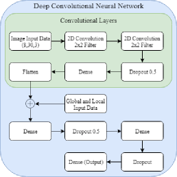
Figure 2: The deep learning architecture using a convolutional neural network combined with a deep neural network. The plus symbol represents the concatenation of data sets.

The input of the CNN is a three-channel MWCG image of dimension (8,30,3). The model then applies two convolutional layers with 2x2 filters followed by a dropout layer at 0.5. This is followed by a dense layer which is flattened then joined with the other global and local features into a dense layer of 59 neurons followed by a dropout layer of 0.5, another dense layer of 100 neurons, a dropout layer of 0.25, a dense layer of 10 neurons, and finishes with a dense layer of 1 neuron. This results in a total of 21,584 trainable parameters for our network.

The convolutional neural network (CNN)has several hyper parameters that can be tuned. In this work we optimize the hyper parameters using the standard practice of a grid search. The parameters used for testing are provided in Table 4. Any hyper parameters not listed below were taken to be the default values provided by the python Keras package.

Table 4: Convolutional Neural Network (CNN) parameters used for testing. Parameters were determined using a grid search. Any hyper parameters not listed below were taken to be the default values provided by python with the Keras package.

Parameter	Setting
Learning Rate	0.001
Epoch	100
Batch Size	100
Loss	Mean Absolute Error
Optimizer	Adam

2.3.4 Training set and test set

The RF, GBT, and CNN were all trained and tested in the same manner. For each protein, a machine learning model is built using the entire dataset but excluding data from the protein whose B-factors are to be predicted. Overall, there are more than 620,000 atoms in our dataset. For each protein, this provides a training set of roughly 600,000 data points (i.e., atoms). For each heavy atom, there is a set of features as described in Section 2.2 and a B-factor value (label). The features and the labels in the training set are used to train each machine learning model. Since we perform leave-one-out predictions, data from each protein is taken as a test set when its B-factors are to be blindly predicted.

We implement random forest and boosted gradient models using the scikit-learn python package. For the CNN model, we also use the python package Keras with tensorflow as a backend.

2.4 Datasets

Our study uses two datasets, one from Park, Jernigan, and Wu [17] and the other from Refs. [12, 13]. The first contains 3 subsets of small, medium, and large proteins [17] and the latter contains 364 proteins [12, 13]. The latter dataset is an extended version of the first. In these proteins, all sequences have a resolution of 3 Å or higher and an average resolution of 1.3 Å and the sets include proteins that range from 4 to 3912 residues [17].

For the CNN the feature datasets were standardized with mean 0 and variance of 1. Proteins 1OB4, 1OB7, 2OLX, and 3MD5 are excluded from the data set because the STRIDE software is unable to provide features for these proteins. We exclude protein 1AGN due to known problems with this protein data. Proteins 1NKO, 2OCT, and 3FVA are also excluded because these proteins have residues with B-factors reported as zero, which is unphysical.

3 Results and discussions

3.1 Evaluation metric

We successfully executed a leave-one-(protein)-out method to blindly predict the B-factors of all carbon, nitrogen, and oxygen atoms present in a given protein. For a comparison with other existing method, we also list results for predicted C_α B-factors, which are predicted in the same way as other heavy atoms. Machine learning was used to train a B-factor prediction model using the structural and B-factor data from a training data set as described in Sections 2.3.4 and 2.4. The model was then used to predict the B-factors of all heavy atoms in a given protein using only its structural data.

To quantitatively assess our method for B-factor prediction we used the Pearson correlation coefficient given by

$${\rm PCC}=\dfrac{\displaystyle\sum_{i=1}^{N}(B_{i}^{e}-\bar{B}^{e})(B_{i}^{t}-\bar{B}^{t})}{\bigg{[}\displaystyle\sum_{i=1}^{N}(B_{i}^{e}-\bar{B}^{e})^{2}\displaystyle\sum_{i=1}^{N}(B_{i}^{t}-\bar{B}^{t})^{2}\bigg{]}^{1/2}},$$ (10)

where $B^{t}_{i},i=1,2,\ldots,N$ are predicted B-factors using the proposed method and $B^{e}_{i},i=1,2,\ldots,N$ experimental B-factors from the PDB file. The terms $B^{t}_{i}$ and $B^{e}_{i}$ represent the $i^{th}$ theoretical and experimental B-factors respectively. Here $\bar{B}^{e}$ and $\bar{B}^{t}$ are averaged B-factors.

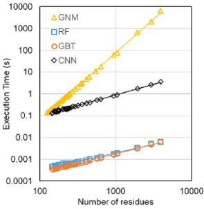
Figure 3: CPU Efficiency comparison between GNM [12], RF, GBT, and CNN algorithms. Execution times in seconds (s) versus number of residues. A set of 34 proteins, listed in Table 5, were used to evaluate the computational complexity.

3.2 Efficiency comparison

Computational efficiency in B-factor predictions is an important consideration for large proteins. Table 5 lists the running times of GNM, RF, GBT, and CNN in our python implementations. These results are depicted in Figure 3. The proteins used to evaluate the computational complexity were the same as those used by Opron et all [12]. For this comparison we only predict B-factors for C_α atoms. Several proteins were excluded as GNM takes significantly too much CPU time to run. Tests excluded the time it took to load PDB files and feature data. The machine learning algorithm times exclude the training of the model, which, once trained, can be used for the prediction of all proteins. The results show that GNM has computational complexity of roughly $\mathcal{O}(N^{3})$ due to the matrix decomposition while the ML algorithms are close to $\mathcal{O}(N)$, with $N$ being the number of atoms. The lines of best fit for CPU time ($t$) are $t\approx(4\times 10^{-8})*N^{3.09}$ for GNM, $t\approx(9\times 10^{-6})*N^{0.78}$ for RF, $t\approx(4\times 10^{-6})*N^{0.87}$ for GBT, and $t\approx(1.1\times 10^{-3})*N^{0.97}$ for CNN.

PDB	N	GNM[12]	RF	GBT	CNN
3P6J	125	0.141	0.000455	0.000358	0.130
3R87	132	0.156	0.000464	0.000339	0.138
3KBE	140	0.187	0.000505	0.000384	0.149
1TZV	141	0.203	0.000473	0.000365	0.163
2VY8	149	0.219	0.000486	0.000359	0.156
3ZIT	152	0.234	0.000519	0.000365	0.148
2FG1	157	0.265	0.000518	0.000403	0.174
2X3M	166	0.312	0.000526	0.000382	0.182
3LAA	169	0.327	0.000514	0.000405	0.155
3M8J	178	0.375	0.000548	0.000412	0.178
2GZQ	191	0.468	0.000647	0.000454	0.195
4G7X	194	0.499	0.000631	0.000445	0.209
2J9W	200	0.546	0.000554	0.000424	0.208
3TUA	210	0.655	0.000602	0.000472	0.217
1U9C	221	0.733	0.000592	0.000486	0.198
3ZRX	221	0.718	0.000654	0.000515	0.216
3K6Y	227	0.765	0.000619	0.000490	0.189
3OQY	234	0.873	0.000619	0.000502	0.211
2J32	244	0.967	0.000625	0.000556	0.225
3M3P	249	1.029	0.000621	0.000525	0.220
1U7I	267	1.263	0.000647	0.000551	0.237
4B9G	292	1.669	0.000693	0.000574	0.256
4ERY	318	2.122	0.000775	0.000619	0.289
3MGN	348	2.902	0.000655	0.000552	0.267
2ZU1	360	3.136	0.000816	0.000675	0.337
2Q52	412	4.696	0.000900	0.000750	0.369
4F01	448	6.178	0.001016	0.000878	0.401
3DRF	547	11.154	0.001131	0.001033	0.512
3UR8	637	17.409	0.001307	0.001136	0.583
2AH1	939	61.012	0.001716	0.001605	0.800
1GCO	1044	75.801	0.001936	0.001814	0.905
1F8R	1932	654.127	0.003343	0.003163	1.745
1H6V	2927	2085.842	0.005205	0.004739	2.543
1QKI	3912	6365.668	0.006261	0.006198	3.560

Table 5: CPU execution times, in seconds, from efficiency comparison between GNM [12], RF, GBT, and CNN.

3.3 Machine learning performance

The results in Table 6 show that for the blind prediction of all heavy atoms the convolutional neural network method performs best with an overall average Pearson correlation coefficient of 0.69. The gradient boosted and random forest ensemble methods performed similarly with Pearson correlation coefficients of 0.63 and 0.59 respectively. For comparison, Table 6 lists only the average Pearson correlation coefficients for C_α B-factor predictions, which are obtained in the same manner as other heavy atoms. These results can be compared with those of the parameter-free flexibility-rigidity index (pfFRI), Gaussian network model (GNM) and normal mode analysis (NMA) which, however, were obtained via the least squares fitting of each protein.

Results for all heavy atom B-factor predictions for small-, medium-, and large-sized protein data subsets [17] are given in Tables 7, 8, and 9. Table LABEL:tab:all shows the results for all heavy atom B-factor predictions of each protein in the Superset. The average Pearson correlation coefficient for the data subsets is provided in Table 6. All methods perform similarly for the different protein data subsets with the convolutional neural network method performing the best on the Superset for both all heavy atom and C_α only B-factor predictions.

Prediction Of Only Cα
Protein Set	RF	GBT	CNN	pfFRI [12]	GNM [12]	NMA [12]
Small	0.25	0.39	0.53	0.60	0.54	0.48
Medium	0.47	0.59	0.55	0.61	0.55	0.48
Large	0.50	0.57	0.62	0.59	0.53	0.49
Superset	0.49	0.57	0.66	0.63	0.57	NA
Prediction Of All Heavy Atom
Protein Set	RF	GBT	CNN	pfFRI [12]	GNM [12]	NMA [12]
Small	0.44	0.49	0.56	NA	NA	NA
Medium	0.59	0.64	0.62	NA	NA	NA
Large	0.62	0.65	0.68	NA	NA	NA
Superset	0.59	0.63	0.69	NA	NA	NA

Table 6: Average Pearson correlation coefficients (PCC) both of all heavy atom and C_α only B-factor predictions for small-, medium-, and large-sized protein sets along with the entire superset of the 364 protein dataset. Predictions of random forest (RF), gradient boosted tree (GBT), and convolutional neural network (CNN) are obtained by leave-one-protein-out (blind), while predictions of parameter-free flexibility-rigidity index (pfFRI), Gaussian network model (GNM) and normal mode analysis (NMA) were obtained via the least squares fitting of individual proteins. All machine learning models use all heavy atom information for training.

Our blind prediction result using the convolutional neural network is notable because it improves upon the best result in the previous work for single protein parameters-free FRI (pfFRI) linear fitting of 0.63 [12]. It is noted that blind predictions are much more difficult than linear fittings. The result for single protein GNM linear fittings of the same data set is 0.57 [12]. As reported in Table LABEL:tab:all, for each protein, no method outperforms any other method over the entire data set. In terms of the average Pearson correlation coefficient for all heavy atom B-factor prediction, the convolutional neural network method outperforms the boosted gradient and random forest by 10% and 17% respectively.

PDB ID	N	RF	GBT	CNN
1AIE	235	0.62	0.53	0.60
1AKG	108	0.41	0.51	0.70
1BX7	345	0.55	0.67	0.63
1ETL	76	0.27	0.03	0.48
1ETM	80	0.46	0.13	0.48
1ETN	77	0.33	0.25	0.20
1FF4	477	0.55	0.59	0.76
1GK7	321	0.53	0.73	0.72
1GVD	401	0.66	0.69	0.71
1HJE	73	-0.07	0.46	0.37
1KYC	138	0.43	0.30	0.32
1NOT	96	-0.18	0.81	0.63
1O06	142	0.51	0.64	0.65
1P9I	203	0.73	0.77	0.77
1PEF	153	0.60	0.64	0.76
1PEN	109	0.34	0.24	0.21
1Q9B	303	0.41	0.67	0.75
1RJU	257	0.71	0.75	0.73
1U06	432	0.55	0.68	0.61
1UOY	452	0.55	0.56	0.55
1USE	290	0.25	0.50	0.68
1VRZ	66	0.38	-0.17	0.09
1XY2	62	0.16	0.27	0.55
1YJO	55	0.36	0.12	0.02
1YZM	361	0.51	0.60	0.56
2DSX	386	0.36	0.44	0.56
2JKU	229	0.57	0.63	0.35
2NLS	269	0.45	0.49	0.70
2OL9	51	0.65	0.51	0.84
6RXN	345	0.56	0.71	0.82

Table 7: Pearson correlation coefficients for cross protein heavy atom blind B-factor prediction obtained by random forest (RF), boosted gradient (GBT), and convolutional neural network (CNN) for the small-sized protein set. Results reported use heavy atoms in both training and prediction.

PDB ID	N	RF	GBT	CNN
1ABA	728	0.74	0.77	0.73
1CYO	697	0.66	0.68	0.76
1FK5	626	0.62	0.71	0.63
1GXU	694	0.65	0.67	0.66
1I71	683	0.57	0.62	0.66
1LR7	522	0.53	0.70	0.71
1N7E	700	0.62	0.65	0.71
1NNX	674	0.69	0.73	0.53
1NOA	778	0.52	0.57	0.57
1OPD	642	0.55	0.60	0.62
1QAU	812	0.57	0.58	0.57
1R7J	729	0.71	0.70	0.65
1UHA	623	0.74	0.80	0.75
1ULR	677	0.69	0.71	0.68
1USM	631	0.59	0.78	0.67
1V05	17	-0.20	0.02	0.60
1W2L	746	0.62	0.68	0.69
1X3O	622	0.53	0.52	0.63
1Z21	771	0.63	0.66	0.63
1ZVA	551	0.59	0.56	0.58
2BF9	287	0.39	0.52	0.70
2BRF	735	0.76	0.78	0.86
2CE0	714	0.62	0.65	0.90
2E3H	589	0.70	0.73	0.38
2EAQ	705	0.63	0.61	0.58
2EHS	590	0.55	0.71	0.38
2FQ3	721	0.67	0.75	0.76
2IP6	702	0.62	0.67	0.64
2MCM	735	0.71	0.73	0.60
2NUH	806	0.64	0.72	0.19
2PKT	666	0.06	0.17	0.76
2PLT	719	0.62	0.67	0.70
2QJL	734	0.61	0.60	0.42
2RB8	723	0.61	0.64	0.42
3BZQ	742	0.60	0.61	0.43
5CYT	800	0.68	0.70	0.74

Table 8: Pearson correlation coefficients for cross protein heavy atom blind B-factor prediction obtained by random forest (RF), boosted gradient (GBT), and convolutional neural network (CNN) for the medium-sized protein set. Results reported use heavy atoms in both training and prediction.

Table 9: Pearson correlation coefficients for cross protein heavy atom blind B-factor prediction obtained by random forest (RF), boosted gradient (GBT), and convolutional neural network (CNN) for the large-sized protein set. Results reported use heavy atoms in both training and prediction.

PDB ID	N	RF	GBT	CNN
1AHO	482	0.62	0.71	0.76
1ATG	1689	0.61	0.66	0.63
1BYI	1540	0.59	0.63	0.59
1CCR	837	0.70	0.67	0.66
1E5K	1423	0.70	0.73	0.74
1EW4	863	0.70	0.71	0.61
1IFR	878	0.72	0.74	0.73
1NLS	1746	0.61	0.64	0.56
1O08	1722	0.51	0.58	0.55
1PMY	937	0.64	0.65	0.67
1PZ4	874	0.73	0.73	0.74
1QTO	934	0.61	0.55	0.63
1RRO	846	0.56	0.52	0.54
1UKU	873	0.74	0.75	0.70
1V70	784	0.70	0.67	0.62
1WBE	1542	0.59	0.61	0.63
1WHI	937	0.74	0.77	0.71
1WPA	906	0.64	0.66	0.74
2AGK	1867	0.61	0.68	0.44
2C71	1446	0.59	0.61	0.83
2CG7	536	0.47	0.54	0.79
2CWS	1624	0.63	0.60	0.78
2HQK	1582	0.76	0.76	0.90
2HYK	1832	0.60	0.65	0.85
2I24	872	0.52	0.52	0.91
2IMF	1564	0.62	0.62	0.47
2PPN	701	0.50	0.68	0.83
2R16	1262	0.52	0.53	0.50
2V9V	986	0.64	0.61	0.63
2VIM	781	0.62	0.61	0.75
2VPA	1524	0.63	0.68	0.61
2VYO	1589	0.53	0.65	0.61
3SEB	1948	0.61	0.71	0.57
3VUB	787	0.64	0.70	0.78

Table 10: Pearson correlation coefficients for cross protein heavy atom blind B-factor prediction obtained by random forest (RF), boosted gradient (GBT), and convolutional neural network (CNN) for the Superset. Results reported use heavy atoms in both training and prediction.

PDB	N	RF	GBT	CNN	PDB	N	RF	GBT	CNN
1ABA	728	0.74	0.77	0.73	2X5Y	1352	0.75	0.79	0.72
1AHO	482	0.62	0.71	0.76	2X9Z	1956	0.71	0.72	0.76
1AIE	235	0.62	0.53	0.60	2XHF	2432	0.65	0.71	0.70
1AKG	108	0.41	0.51	0.70	2Y0T	757	0.59	0.75	0.73
1ATG	1689	0.61	0.66	0.63	2Y72	1171	0.73	0.80	0.75
1BGF	1018	0.58	0.63	0.63	2Y7L	2398	0.81	0.82	0.62
1BX7	345	0.55	0.67	0.63	2Y9F	1212	0.72	0.77	0.64
1BYI	1540	0.59	0.63	0.59	2YLB	3065	0.60	0.69	0.63
1CCR	837	0.70	0.67	0.66	2YNY	2364	0.67	0.71	0.68
1CYO	697	0.66	0.68	0.76	2ZCM	2959	0.41	0.45	0.44
1DF4	463	0.79	0.75	0.64	2ZU1	2794	0.59	0.73	0.17
1E5K	1423	0.70	0.73	0.74	3A0M	823	0.65	0.47	0.74
1ES5	1912	0.63	0.68	0.66	3A7L	963	0.66	0.75	0.81
1ETL	76	0.27	0.03	0.48	3AMC	5174	0.72	0.75	0.62
1ETM	80	0.46	0.13	0.48	3AUB	782	0.63	0.62	0.74
1ETN	77	0.33	0.25	0.20	3B5O	1510	0.53	0.55	0.65
1EW4	863	0.70	0.71	0.61	3BA1	2391	0.65	0.64	0.44
1F8R	15291	0.64	0.64	0.83	3BED	1570	0.73	0.73	0.70
1FF4	477	0.55	0.59	0.76	3BQX	1028	0.52	0.59	0.85
1FK5	626	0.62	0.71	0.63	3BZQ	742	0.60	0.61	0.43
1GCO	7888	0.64	0.61	0.71	3BZZ	773	0.45	0.45	0.77
1GK7	321	0.53	0.73	0.72	3DRF	4101	0.67	0.66	0.81
1GVD	401	0.66	0.69	0.71	3DWV	2363	0.60	0.67	0.87
1GXU	694	0.65	0.67	0.66	3E5T	1543	0.71	0.72	0.75
1H6V	22514	0.39	0.40	0.58	3E7R	295	0.60	0.60	0.81
1HJE	73	-0.07	0.46	0.37	3EUR	1059	0.47	0.50	0.82
1I71	683	0.57	0.62	0.66	3F2Z	1160	0.78	0.78	0.88
1IDP	3661	0.69	0.74	0.83	3F7E	1912	0.61	0.67	0.69
1IFR	878	0.72	0.74	0.73	3FCN	1039	0.68	0.71	0.73
1K8U	686	0.65	0.68	0.74	3FE7	710	0.62	0.71	0.83
1KMM	11632	0.65	0.70	0.87	3FKE	1938	0.57	0.56	0.76
1KNG	1016	0.61	0.56	0.55	3FMY	470	0.73	0.75	0.84
1KR4	906	0.73	0.76	0.72	3FOD	328	0.30	0.45	0.78
1KYC	138	0.43	0.30	0.32	3FSO	197	0.71	0.73	0.85
1LR7	522	0.53	0.70	0.71	3FTD	1795	0.75	0.75	0.69
1MF7	1551	0.68	0.68	0.70	3G1S	3196	0.74	0.76	0.72
1N7E	700	0.62	0.65	0.71	3GBW	1275	0.75	0.76	0.68
1NKD	426	0.56	0.59	0.63	3GHJ	808	0.66	0.71	0.44
1NLS	1746	0.61	0.64	0.56	3HFO	1432	0.65	0.72	0.70
1NNX	674	0.69	0.73	0.53	3HHP	8495	0.71	0.74	0.62
1NOA	778	0.52	0.57	0.57	3HNY	1351	0.73	0.73	0.58
1NOT	96	-0.18	0.81	0.63	3HP4	1322	0.61	0.63	0.65
1O06	142	0.51	0.64	0.65	3HWU	934	0.51	0.69	0.51
1O08	1722	0.51	0.58	0.55	3HYD	52	-0.05	0.28	0.60
1OPD	642	0.55	0.60	0.62	3HZ8	1459	0.51	0.54	0.76
1P9I	203	0.73	0.77	0.77	3I2V	929	0.50	0.54	0.81
1PEF	153	0.60	0.64	0.76	3I2Z	1039	0.63	0.64	0.75
1PEN	109	0.34	0.24	0.21	3I4O	969	0.66	0.64	0.87
1PMY	937	0.64	0.65	0.67	3I7M	928	0.56	0.60	0.87
1PZ4	874	0.73	0.73	0.74	3IHS	1120	0.66	0.65	0.81
1Q9B	303	0.41	0.67	0.75	3IVV	1097	0.72	0.81	0.85
1QAU	812	0.57	0.58	0.57	3K6Y	1617	0.62	0.65	0.90
1QKI	31154	0.44	0.27	0.84	3KBE	829	0.75	0.76	0.86
1QTO	934	0.61	0.55	0.63	3KGK	1492	0.75	0.78	0.87
1R29	971	0.61	0.73	0.72	3KZD	605	0.64	0.70	0.74
1R7J	729	0.71	0.70	0.65	3L41	1735	0.73	0.76	0.88
1RJU	257	0.71	0.75	0.73	3LAA	1112	0.54	0.46	0.89
1RRO	846	0.56	0.52	0.54	3LAX	753	0.69	0.71	0.89
1SAU	830	0.62	0.68	0.60	3LG3	6061	0.57	0.59	0.91
1TGR	749	0.61	0.65	0.67	3LJI	1946	0.46	0.54	0.50
1TZV	1051	0.75	0.77	0.75	3M3P	1858	0.57	0.62	0.68
1U06	432	0.55	0.68	0.61	3M8J	1396	0.78	0.77	0.68
1U7I	1988	0.73	0.75	0.77	3M9J	1329	0.66	0.74	0.50
1U9C	1712	0.61	0.64	0.58	3M9Q	1359	0.52	0.53	0.48
1UHA	623	0.74	0.80	0.75	3MAB	1311	0.63	0.65	0.59
1UKU	873	0.74	0.75	0.70	3MD4	81	0.36	0.61	0.79
1ULR	677	0.69	0.71	0.68	3MEA	1236	0.58	0.64	0.93
1UOY	452	0.55	0.56	0.55	3MGN	2236	0.15	0.03	0.82
1USE	290	0.25	0.50	0.68	3MRE	2598	0.57	0.56	0.84
1USM	631	0.59	0.78	0.67	3N11	2501	0.52	0.57	0.85
1UTG	548	0.58	0.55	0.62	3NE0	1551	0.68	0.69	0.85
1V05	17	-0.20	0.02	0.60	3NGG	702	0.63	0.75	0.83
1V70	784	0.70	0.67	0.62	3NPV	3655	0.70	0.75	0.84
1VRZ	66	0.38	-0.17	0.09	3NVG	50	-0.08	0.08	0.88
1W2L	746	0.62	0.68	0.69	3NZL	567	0.59	0.65	0.63
1WBE	1542	0.59	0.61	0.63	3O0P	1452	0.55	0.65	0.63
1WHI	937	0.74	0.77	0.71	3O5P	819	0.53	0.63	0.70
1WLY	2430	0.65	0.71	0.68	3OBQ	1195	0.61	0.61	0.84
1WPA	906	0.64	0.66	0.74	3OQY	1772	0.57	0.62	0.76
1X3O	622	0.53	0.52	0.63	3P6J	857	0.57	0.70	0.88
1XY1	124	0.58	0.19	0.47	3PD7	1354	0.70	0.72	0.85
1XY2	62	0.16	0.27	0.55	3PES	1240	0.72	0.73	0.84
1Y6X	669	0.44	0.53	0.46	3PID	3078	0.49	0.56	0.86
1YJO	55	0.36	0.12	0.02	3PIW	1223	0.72	0.75	0.87
1YZM	361	0.51	0.60	0.56	3PKV	1688	0.66	0.68	0.81
1Z21	771	0.63	0.66	0.63	3PSM	729	0.62	0.68	0.80
1ZCE	1100	0.77	0.81	0.73	3PTL	2101	0.61	0.62	0.72
1ZVA	551	0.59	0.56	0.58	3PVE	2656	0.56	0.61	0.46
2A50	3493	0.64	0.48	0.68	3PZ9	2913	0.63	0.76	0.60
2AGK	1867	0.61	0.68	0.44	3PZZ	76	0.47	0.25	0.85
2AH1	7215	0.65	0.57	0.67	3Q2X	43	0.29	0.59	0.76
2B0A	1454	0.66	0.68	0.72	3Q6L	1022	0.71	0.67	0.75
2BCM	3002	0.51	0.62	0.85	3QDS	2234	0.71	0.72	0.71
2BF9	287	0.39	0.52	0.70	3QPA	1348	0.43	0.44	0.71
2BRF	735	0.76	0.78	0.86	3R6D	1550	0.31	0.69	0.59
2C71	1446	0.59	0.61	0.83	3R87	1007	0.39	0.51	0.53
2CE0	714	0.62	0.65	0.90	3RQ9	1174	0.32	0.47	0.66
2CG7	536	0.47	0.54	0.79	3RY0	964	0.66	0.65	0.53
2COV	4366	0.76	0.83	0.78	3RZY	985	0.69	0.69	0.64
2CWS	1624	0.63	0.60	0.78	3S0A	884	0.55	0.61	0.61
2D5W	9772	0.71	0.75	0.75	3SD2	527	0.38	0.52	0.71
2DKO	1933	0.71	0.72	0.72	3SEB	1948	0.61	0.71	0.57
2DPL	4454	0.49	0.53	0.73	3SED	933	0.70	0.71	0.72
2DSX	386	0.36	0.44	0.56	3SO6	1119	0.69	0.75	0.01
2E10	3416	0.50	0.64	0.61	3SR3	4891	0.69	0.69	0.45
2E3H	589	0.70	0.73	0.38	3SUK	1761	0.62	0.65	0.59
2EAQ	705	0.63	0.61	0.58	3SZH	5074	0.74	0.80	0.44
2EHP	1875	0.75	0.74	0.74	3T0H	1627	0.78	0.81	0.65
2EHS	590	0.55	0.71	0.38	3T3K	922	0.56	0.68	0.62
2ERW	385	0.47	0.50	0.32	3T47	1116	0.54	0.62	0.74
2ETX	3018	0.56	0.61	0.58	3TDN	2703	0.55	0.55	0.58
2FB6	766	0.63	0.65	0.52	3TOW	1193	0.53	0.66	0.66
2FG1	1021	0.55	0.65	0.68	3TUA	1510	0.63	0.66	0.70
2FN9	4362	0.37	0.60	0.61	3TYS	556	0.67	0.68	0.71
2FQ3	721	0.67	0.75	0.76	3U6G	1658	0.52	0.51	0.60
2G69	744	0.60	0.61	0.87	3U97	524	0.57	0.66	0.27
2G7O	537	0.52	0.63	0.89	3UCI	536	0.44	0.51	0.56
2G7S	1258	0.60	0.60	0.81	3UR8	5033	0.63	0.66	0.83
2GKG	706	0.63	0.60	0.70	3US6	1156	0.62	0.64	0.01
2GOM	987	0.61	0.70	0.92	3V1A	319	0.36	0.36	0.76
2GXG	1132	0.67	0.75	0.86	3V75	1974	0.63	0.65	0.83
2GZQ	1402	0.59	0.60	0.90	3VN0	1469	0.69	0.76	0.76
2HQK	1582	0.76	0.76	0.90	3VOR	1077	0.41	0.50	0.81
2HYK	1832	0.60	0.65	0.85	3VUB	787	0.64	0.70	0.78
2I24	872	0.52	0.52	0.91	3VVV	869	0.62	0.69	0.84
2I49	3109	0.78	0.77	0.90	3VZ9	1366	0.70	0.72	0.66
2IBL	815	0.46	0.53	0.88	3W4Q	5406	0.66	0.73	0.65
2IGD	431	0.58	0.68	0.82	3ZBD	1718	0.54	0.54	0.78
2IMF	1564	0.62	0.62	0.47	3ZIT	1192	0.51	0.54	0.71
2IP6	702	0.62	0.67	0.64	3ZRX	1654	0.38	0.67	0.60
2IVY	727	0.47	0.59	0.62	3ZSL	925	0.61	0.64	0.69
2J32	1935	0.79	0.78	0.70	3ZZP	585	0.40	0.46	0.56
2J9W	1626	0.66	0.68	0.73	3ZZY	1741	0.64	0.69	0.69
2JKU	229	0.57	0.63	0.35	4A02	1281	0.62	0.65	0.75
2JLI	708	0.58	0.54	0.73	4ACJ	1210	0.64	0.67	0.75
2JLJ	889	0.66	0.70	0.68	4AE7	1458	0.64	0.74	0.61
2MCM	735	0.71	0.73	0.60	4AM1	2605	0.64	0.67	0.56
2NLS	269	0.45	0.49	0.70	4ANN	1180	0.53	0.60	0.72
2NR7	1556	0.71	0.70	0.66	4AVR	1437	0.62	0.61	0.64
2NUH	806	0.64	0.72	0.19	4AXY	317	0.45	0.64	0.75
2O6X	2415	0.76	0.82	0.63	4B6G	4504	0.78	0.76	0.84
2OA2	970	0.54	0.53	0.92	4B9G	2226	0.79	0.81	0.83
2OHW	2074	0.55	0.62	0.81	4DD5	2618	0.63	0.66	0.87
2OKT	2587	0.56	0.59	0.89	4DKN	3356	0.76	0.77	0.88
2OL9	51	0.65	0.51	0.84	4DND	755	0.66	0.73	0.85
2PKT	666	0.06	0.17	0.76	4DPZ	865	0.65	0.66	0.83
2PLT	719	0.62	0.67	0.70	4DQ7	2526	0.58	0.69	0.78
2PMR	590	0.63	0.66	0.63	4DT4	1163	0.71	0.73	0.73
2POF	3418	0.58	0.66	0.85	4EK3	2147	0.70	0.72	0.73
2PPN	701	0.50	0.68	0.83	4ERY	2357	0.70	0.74	0.83
2PSF	4983	0.54	0.55	0.79	4ES1	737	0.63	0.64	0.81
2PTH	1437	0.68	0.72	0.79	4EUG	1789	0.59	0.66	0.79
2Q4N	9496	0.45	0.39	0.85	4F01	3374	0.55	0.54	0.77
2Q52	26784	0.63	0.62	0.77	4F3J	1116	0.58	0.62	0.53
2QJL	734	0.61	0.60	0.42	4FR9	956	0.61	0.64	0.62
2R16	1262	0.52	0.53	0.50	4G14	39	0.28	0.50	0.55
2R6Q	903	0.59	0.53	0.57	4G2E	1178	0.73	0.73	0.76
2RB8	723	0.61	0.64	0.42	4G5X	4002	0.74	0.75	0.65
2RE2	1559	0.66	0.66	0.54	4G6C	4814	0.47	0.60	0.61
2RFR	1019	0.54	0.58	0.66	4G7X	1315	0.49	0.56	0.80
2V9V	986	0.64	0.61	0.63	4GA2	873	0.51	0.55	0.55
2VE8	3967	0.65	0.59	0.66	4GMQ	678	0.56	0.72	0.54
2VH7	749	0.74	0.70	0.82	4GS3	737	0.56	0.60	0.56
2VIM	781	0.62	0.61	0.75	4H4J	1470	0.69	0.80	0.70
2VPA	1524	0.63	0.68	0.61	4H89	1127	0.55	0.61	0.62
2VQ4	800	0.72	0.76	0.78	4HDE	1288	0.73	0.79	0.70
2VY8	1058	0.71	0.74	0.63	4HJP	2112	0.65	0.70	0.76
2VYO	1589	0.53	0.65	0.61	4HWM	799	0.50	0.57	0.81
2W1V	4223	0.68	0.72	0.72	4IL7	527	0.35	0.43	0.74
2W2A	2918	0.56	0.62	0.63	4J11	2658	0.47	0.58	0.94
2W6A	826	0.66	0.76	0.69	4J5O	1406	0.64	0.63	0.91
2WJ5	630	0.49	0.53	0.77	4J5Q	1062	0.73	0.75	0.87
2WUJ	828	0.55	0.55	0.55	4J78	2443	0.71	0.75	0.86
2WW7	915	0.35	0.43	0.61	4JG2	1294	0.70	0.73	0.88
2WWE	54	0.23	0.22	0.12	4JVU	1615	0.69	0.68	0.89
2X1Q	1852	0.58	0.53	0.77	4JYP	4063	0.70	0.78	0.93
2X25	1289	0.65	0.68	0.80	4KEF	1002	0.65	0.62	0.68
2X3M	1267	0.66	0.70	0.75	5CYT	800	0.68	0.70	0.74
					6RXN	345	0.56	0.71	0.82

Some low Pearson correlation coefficients results show a poor model prediction. However, in almost every protein where one model performs poorly, another model performs satisfactorily. When the maximum correlation coefficient for each protein is considered among the three methods the average all heavy atom correlation coefficient is increased to 0.73 and the average C_α only correlation coefficient is increased to 0.72. This result is similar to that of the parameter-optimized FRI (opFRI) reported in our earlier work [12].

3.4 Relative feature importance

Both random forest and boosted gradient methods have the ability to rank relative feature importance helping us understand significant features in the model. Figure 4 shows the individual feature importance for the random forest averaged over the dataset.

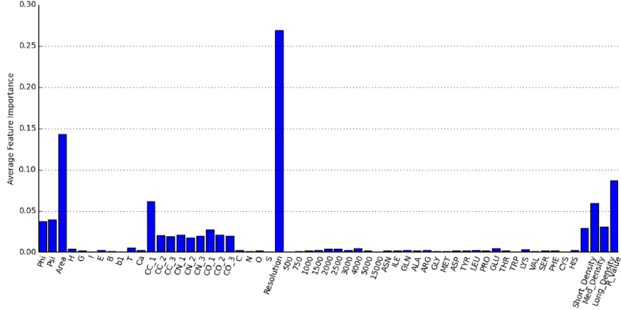
Figure 4: Individual feature importance for the random forest model averaged over the data set. Reported feature selection includes the use heavy atoms in the model.

We also include aggregated feature importance in Figure 5. In this figure, we sum the importance of the individual angle, secondary, MWCG, atom type, protein size, amino acid, and packing density features.

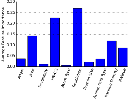
Figure 5: Average feature importance for the random forest model with the angle, secondary, MWCG, atom type, protein size, amino acid, and packing density features aggregated. Reported feature selection includes the use heavy atoms in the model.

Figure 4 shows the most important MWCG feature is the carbon-carbon interaction. This MWCG feature uses a Lorentz radial basis function as with $\eta=16$ and $\nu=3$ as detailed in Section 2.2. The remaining eight MWCG features all rank similarly with the carbon-oxygen interaction ranked as the second most significant MWCG feature. This result validates that the model benefits from the multi-scale property of the MWCG feature, which uses three different kernels to capture interactions at various length scales. Since all MWCG have significance in the feature ranking it follows that the element specific property of the MWCG method is also a meaningful model feature.

Figure 4 shows that that the individual MWCG, amino acid type, and packing density feature have low relative importance, however, considering their aggregate importance as seen in Figure 5, we see that they contribute to the model. Figure 5 shows that the medium density protein packing density feature was twice as important to the model as the short and long density features. The medium packing density may be capturing semi-local side chain interactions which are important in protein flexibility. The short packing density likely captures only adjacent backbone information while the long packing density is only adding weak atomic interaction information to the model. Protein resolution is the most significant relative feature followed by MWCG features and the STRIDE generated residue solvent accessible area feature. This also highlights the importance of the quality of X-ray crystal structures and difficulty in cross-protein B-factor prediction. Protein angles, secondary structures, and size play a less significant role in the model compared to the other features. Atom type has the lowest significance relative to the other features implemented in the model. Not surprisingly, we see that global features such as resolution and R-value are important components in the ensemble model. The global feature of protein size has a small role in the model.

Care must be taken to use feature ranking to understand feature importance. The feature ranking provided by these models is a relative ordering of features that the models find most important. So features with high correlation may be redundant giving one of them a lower rank even though they may have significant prediction power. For example, R-value highly correlates with resolution so it is likely a meaningful feature. However, the use of resolution reduces the relative importance ranking of R-value in the model.

3.5 Machine learning methods

Among the three methods considered in this work, the convolutional neural network method outperforms the boosted gradient tree and random forest by 10% and 17%, respectively. As reported in Table LABEL:tab:all, no machine learning method outperforms any other method for each of all proteins. Results for all machine learning methods could undoubtedly be improved by refining features, exploring new features, and further tuning hyperparameters.

In general, ensemble methods do not require as much parameter tuning as the CNN does. The random forest is the simplest and most robust method. To balance cost, time, and quality only 500 trees were used for the random forest and 1000 trees were used for the boosted gradient method in this work. This may account for the increased performance of the boosted gradient tree method compared to the random forest. Ensemble methods are quite robust against overfitting so adding more features would likely improve their results [18]. The boosted gradient trees use several hyperparameters so these methods could benefit by further tuning these hyperparameters.

The additional data in the form of MWCG images used in the convolutional neural network likely explains the improved performance as compared to the ensemble methods. More refined images and other novel image types could further improve results.

Using the dropout strategy, CNNs are also robust against overfitting. Since there are a few hyperparameters in the CNN method, it would likely benefit from more detailed parameter tuning. Additionally, a large dataset and more features would also improve the CNN performance. For example, including persistent homology [19] and differential geometry features might lead to a better CNN prediction.

4 Conclusion

Protein flexibility is known to strongly correlate with protein function and its prediction is important for our understanding of protein dynamics and transport. Our quantitative understanding of protein flexibility and function is greatly impeded by their complexity and a large number of degrees of freedom. Many time-independent methods, such as NMA [4, 20, 5, 3], ENM [6], GNM [8, 9, 21], and FRI [11, 12, 13, 22], exist that dramatically simplify the protein structural complexity and are able to analyze protein B-factors, which reflect protein flexibility among other things. Based on the hypothesis that intrinsic physics lies in a low-dimensional space embedded in a high-dimensional data space, we introduced multiscale weighted colored graphs (MWCGs) to effectively reduce protein structural complexity and efficiently describe protein flexibility. However, none of the aforementioned methods is able to blindly predict the protein B-factors of an unknown protein. This work integrates advanced machine learning algorithms and two sets of features, i.e., global and local ones, to blindly predict protein flexibility and B-factors.

A few standard datasets involving more than 300 proteins (or more than 600,000 of B-factors) have been utilized to test the proposed method. We use the leave-one-protein-out scheme to blindly predict protein B-factors of both all heavy atoms and only C_α atoms. Extensive numerical experiments demonstrate that the present blind prediction is more accurate than the least squares fitting using GNM or NMA in terms of Pearson’s correlation coefficients for the prediction of C_α B-factor. Further, we demonstrate the ability to effectively blindly predict B-factors of any heavy atoms in a given protein.

Three standard machine learning algorithms, namely, the random forest, graduate boosted trees, and convolutional neural networks are employed in the present study. Among them, convolutional neural networks do a better job in B-factor predictions. A variety of different features were considered for these models including local, semi-local, and global features. Local features, such as MWCGs, are designed to capture structural properties associated with the intrinsic flexibility while global features, such as X-ray crystal resolution, are used to enable the cross-protein comparison and analysis. The proposed method is very efficient. However, there is still much room for novel and interesting features that can be implemented in future work. For example, many algebraic topology tools have been found very useful for protein analysis [23, 18, 19] and will likely pair well with machine learning approaches for protein flexibility predictions.

This work is a first step using the recent advances in machine learning techniques to blindly predict protein B-factors. To the authors’ knowledge, this is the first work demonstrating this as a feasible and robust prediction method. This work provides a clear evidence that machine algorithms are useful in protein flexibility analysis. Results for all methods could undoubtedly be improved by a better mathematical description of intrinsic flexibility, larger datasets, and more advanced machine learning algorithms.

The proposed methods could be implemented in a variety of interesting applications related to protein flexibility and function. These include topics such as hinge detection, hot spot identification, allosteric site detection, pose prediction, protein folding, and computer-aided drug design.

References

- [1] J. P. Ma, “Usefulness and limitations of normal mode analysis in modeling dynamics of biomolecular complexes.,” Structure, vol. 13, pp. 373 – 180, 2005.
- [2] H. Frauenfelder, S. G. Slihar, and P. G. Wolynes, “ The energy landsapes and motion of proteins ,” Science, vol. 254, pp. 1598–1603, DEC 13 1991.
- [3] M. Tasumi, H. Takenchi, S. Ataka, A. M. Dwidedi, and S. Krimm, “Normal vibrations of proteins: Glucagon,” Biopolymers, vol. 21, pp. 711 – 714, 1982.
- [4] B. R. Brooks, R. E. Bruccoleri, B. D. Olafson, D. States, S. Swaminathan, and M. Karplus, “Charmm: A program for macromolecular energy, minimization, and dynamics calculations,” J. Comput. Chem., vol. 4, pp. 187–217, 1983.
- [5] M. Levitt, C. Sander, and P. S. Stern, “Protein normal-mode dynamics: Trypsin inhibitor, crambin, ribonuclease and lysozyme.,” J. Mol. Biol., vol. 181, no. 3, pp. 423 – 447, 1985.
- [6] M. M. Tirion, “Large amplitude elastic motions in proteins from a single-parameter, atomic analysis.,” Phys. Rev. Lett., vol. 77, pp. 1905 – 1908, 1996.
- [7] A. R. Atilgan, S. R. Durrell, R. L. Jernigan, M. C. Demirel, O. Keskin, and I. Bahar, “Anisotropy of fluctuation dynamics of proteins with an elastic network model.,” Biophys. J., vol. 80, pp. 505 – 515, 2001.
- [8] I. Bahar, A. R. Atilgan, and B. Erman, “Direct evaluation of thermal fluctuations in proteins using a single-parameter harmonic potential.,” Folding and Design, vol. 2, pp. 173 – 181, 1997.
- [9] I. Bahar, A. R. Atilgan, M. C. Demirel, and B. Erman, “Vibrational dynamics of proteins: Significance of slow and fast modes in relation to function and stability.,” Phys. Rev. Lett, vol. 80, pp. 2733 – 2736, 1998.
- [10] T. Haliloglu, I. Bahar, and B. Erman, “Gaussian dynamics of folded proteins,” Physical review letters, vol. 79, no. 16, p. 3090, 1997.
- [11] K. L. Xia and G. W. Wei, “A stochastic model for protein flexibility analysis,” Physical Review E, vol. 88, p. 062709, 2013.
- [12] K. Opron, K. L. Xia, and G. W. Wei, “Fast and anisotropic flexibility-rigidity index for protein flexibility and fluctuation analysis,” Journal of Chemical Physics, vol. 140, p. 234105, 2014.
- [13] K. Opron, K. L. Xia, and G. W. Wei, “Communication: Capturing protein multiscale thermal fluctuations,” Journal of Chemical Physics, vol. 142, no. 211101, 2015.
- [14] D. D. Nguyen, K. L. Xia, and G. W. Wei, “Generalized flexibility-rigidity index,” Journal of Chemical Physics, vol. 144, p. 234106, 2016.
- [15] D. Bramer and G.-W. Wei, “Multiscale weighted colored graphs for protein flexibility and rigidity analysis,” The Journal of Chemical Physics, vol. 148, no. 5, p. 054103, 2018.
- [16] M. Heinig and D. Frishman, “Stride: a web server for secondary structure assignment from known atomic coordinates of proteins,” Nucleic Acids Research, vol. 32, no. suppl 2, pp. W500–W502, 2004.
- [17] J. K. Park, R. Jernigan, and Z. Wu, “Coarse grained normal mode analysis vs. refined gaussian network model for protein residue-level structural fluctuations,” Bulletin of Mathematical Biology, vol. 75, pp. 124 –160, 2013.
- [18] Z. X. Cang and G. W. Wei, “Analysis and prediction of protein folding energy changes upon mutation by element specific persistent homology,” Bioinformatics, vol. 33, pp. 3549–3557, 2017.
- [19] Z. X. Cang and G. W. Wei, “Integration of element specific persistent homology and machine learning for protein-ligand binding affinity prediction ,” International Journal for Numerical Methods in Biomedical Engineering, vol. 34, p. 22914, 2018.
- [20] N. Go, T. Noguti, and T. Nishikawa, “Dynamics of a small globular protein in terms of low-frequency vibrational modes,” Proc. Natl. Acad. Sci., vol. 80, pp. 3696 – 3700, 1983.
- [21] B. Brooks and M. Karplus, “Harmonic dynamics of proteins: normal modes and fluctuations in bovine pancreatic trypsin inhibitor,” Proceedings of the National Academy of Sciences, vol. 80, no. 21, pp. 6571–6575, 1983.
- [22] K. Opron, K. L. Xia, Z. Burton, and G. W. Wei, “Flexibility-rigidity index for protein-nucleic acid flexibility and fluctuation analysis,” Journal of Computational Chemistry, vol. 37, pp. 1283–1295, 2016.
- [23] K. L. Xia and G. W. Wei, “Persistent homology analysis of protein structure, flexibility and folding,” International Journal for Numerical Methods in Biomedical Engineering, vol. 30, pp. 814–844, 2014.