Reinforcement Learning in Topology-based Representation for
Human Body Movement with Whole Arm Manipulation

Abstract

Moving a human body or a large and bulky object can require the strength of whole arm manipulation (WAM). This type of manipulation places the load on the robot’s arms and relies on global properties of the interaction to succeed—rather than local contacts such as grasping or non-prehensile pushing. In this paper, we learn to generate motions that enable WAM for holding and transporting of humans in certain rescue or patient care scenarios. We model the task as a reinforcement learning problem in order to provide a behavior that can directly respond to external perturbation and human motion. For this, we represent global properties of the robot-human interaction with topology-based coordinates that are computed from arm and torso positions. These coordinates also allow transferring the learned policy to other body shapes and sizes. For training and evaluation, we simulate a dynamic sea rescue scenario and show in quantitative experiments that the policy can solve unseen scenarios with differently-shaped humans, floating humans, or with perception noise. Our qualitative experiments show the subsequent transporting after holding is achieved and we demonstrate that the policy can be directly transferred to a real world setting.

I INTRODUCTION

Robotic manipulation is a complex problem that is often approached by grasping [1, 2] or non-prehensile pushing [3, 4, 5]. However, when heavy or bulky objects need to be manipulated whole arm manipulation (WAM) is usually much more suitable [6, 7, 8, 9]. In WAM the robot’s arms instead of its sensitive end-effectors are used to carry the load or provide support. This type of interaction is also often observed when somebody moves an injured person [9] or rescues a drowning person at sea. Here, one or both arms are employed to embrace the person’s body and then hold and transport the person as seen in Fig. 1.

In this paper, we learn to generate motions that enable WAM for holding and transporting of humans in certain rescue or patient care scenarios. This is a challenging WAM problem because humans have different sizes and shapes and can move and change their pose during interaction which is difficult to predict and model. Furthermore, a robot that is strong enough to move a person can easily cause injury. WAM has previously been considered from the perspective of mechanical design [10, 11], robot control [7, 12, 13] and modeling of interaction [14]. In contrast to these works, we consider generating WAM-motions with a model-free learning-based approach and leave execution to a low-level controller.

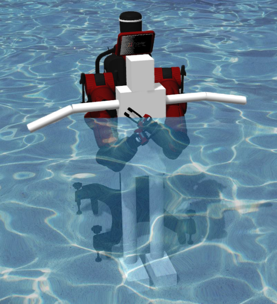
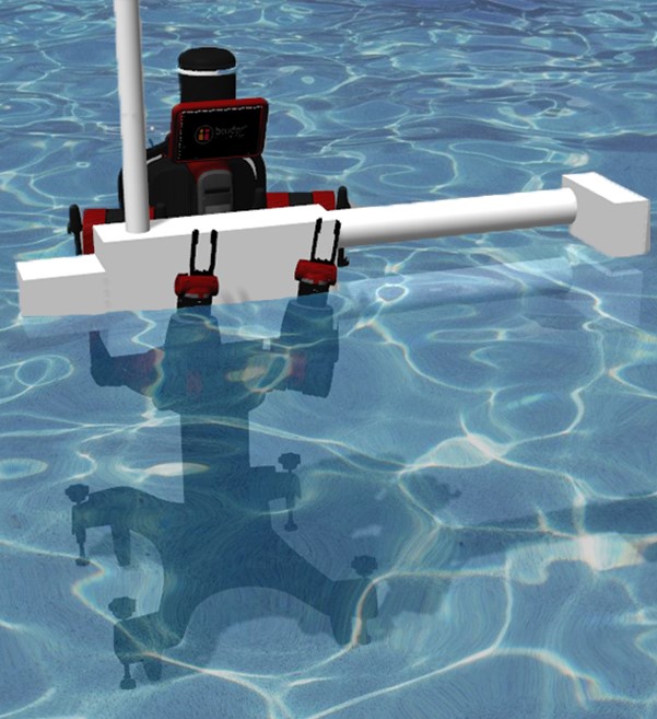
(a) Upright	(b) Horizontal

Figure 1: For a swimming rescue the robot has to firmly hold and then transport the drowning person which needs the strength of whole arm interaction. During the rescue, the person keeps move up and down due to waves and the robot has to continuously react to these changes.

Our scenarios require close interaction between the bodies of a humanoid robot and a person. This interaction is difficult to formalize for planning and control because of variation in geometry and uncertainty about physical response to contact forces. Moreover, the success of this interaction depends on global properties which are difficult to determine geometrically, such as the form of entanglement between the two bodies. Instead of referring to geometry, such as angles and positions of limbs, the magnitude of entanglement between limbs has therefore been considered for generating motions of two humanoid actors [15, 16]. This topology-based representation called Writhe matrix generalizes well to certain changes in body shape, size or their relative pose and we therefore employ it to capture the relationship of the two humanoid bodies in our scenarios.

Several works leverage Writhe matrix coordinates for generating motions: Ho et al. interpolate between a set of key-poses and sequence more complex interactions with a state machine [15, 16], Stork et al. use sampling-based planning to generate caging-grasps [17, 18], and Ivan et al. present a control framework for motion planning [19]. For our scenarios, these approaches are not flexible enough because they require defining the interaction using intermediate goals or do not continuously react to changes in the environment, such as waves during a swimming rescue. Instead, we employ model-free reinforcement learning to obtain a policy that can generate the desired motion.

In this context, we exploit the topology-based representation in two ways: Because of its invariance properties, we only have to train for one humanoid body shape and can apply the policy to humans of different shapes and sizes. Further, since the representation is based only on a simplified skeleton of the body, we can train in a virtual environment and apply the policy in reality without adaption as long as such a skeleton can be provided in the real scene.

Our contributions in this work are:

• formulating motion generation for WAM as a reinforcement learning problem and thus enabling reactive behavior,

• exploiting Writhe and Laplacian coordinates in reinforcement learning of WAM interaction with humans,

• modeling of two different dual-arm scenarios: interaction with upright and horizontal humanoid.

Our evaluation shows that we can reliably learn a policy that can generate the desired motion for different scenarios with a high success rate of $99\%$. In evaluation with humanoid bodies of different shapes and sizes, bodies in continuous motion, and artificial perception noise, the policy still performs well. Additionally, we show a proof-of-concept for applying the policy in reality with a real robot and person.

II RELATED WORK

In this section, we first review the works where robots use their arms to hold heavy or bulky objects and then survey learning methods that are similar to our approach.

The classical approach to manipulating bulky objects is based on physical modeling. For instance, Kaneko et al. analyze forces and moments between the robot’s legs and the object in order to maintain static balance [20]. Similarly, Florek-Jasińska et al. propose an impedance controller to use contacts at both arms and the robot’s chest to grasp a large object [7]. Different to these works, we do not consider contact forces since these are difficult to model for WAM interaction with humans. Instead we are interested in the spacial relationship between robot and human.

Marzinotto et al. maximize Writhe between robot arms and a tunnel hole in the object for collaborative grasping and transport of a large object [18]. The representation and task formulation is similar to other works where Writhe or Linking is considered for caging grasps [21, 22, 17], motion planning through holes [23, 19], or animation of humanoid characters [15, 24]. Similar to these works, we employ topology-based coordinates and aim to maximize the linking value between the robot and the person to reach a starting pose for transport. However, instead of sampling-based planning or optimal control which are time-consuming and not suitable for dynamic scenarios, we use reinforcement learning to find a policy which maximizes the linking value.

Since deep reinforcement learning has shown success in complex artificial domains [25, 26], controlling robots with reinforcement learning has become increasingly interesting [27]. For instance, it has been used to learn grasping [28, 29] or manipulation in dynamic environments [5, 30]. While these works exploit the advantages of deep models for visual input, this makes it difficult for them to generalize to different conditions. In contrast to that, we use topology-based coordinates as input to our policy. These coordinates are an abstraction for the actual shape and appearance of the robot and human and therefore intrinsically allow for generalization to different shapes and sizes.

III TOPOLOGICAL REPRESENTATION

In this section, we describe how we represent the robot-humanoid relationship for our WAM scenario. This representation serves as input to the reinforcement learning policy described in Sec. IV. We employ the concepts of Writhe matrix and Laplacian coordinates which we explain in Sec. III-A and Sec. III-B before we define our representation in Sec. III-C.

III-A Writhe Matrix

The Writhe matrix $W$ with the entries $W_{i,j}$ is a representation of how much two curves, $\gamma_{1}$ and $\gamma_{2}$, wind around each other in three-dimensional space [15]. While the Gaussian linking integral $\Gamma(\gamma_{1},\gamma_{2})$ represents this property as a single scalar [31],

$$\Gamma(\gamma_{1},\gamma_{2})=\frac{1}{4\pi}\int_{\gamma_{1}}\int_{\gamma_{2}}\frac{d\gamma_{1}\times d\gamma_{2}\cdot(\gamma_{1}-\gamma_{2})}{\|\gamma_{1}-\gamma_{2}\|^{3}},$$ (1)

the Writhe matrix records this information separately for different segments of the two curves. For this, both curves are approximated with two sequences of line segments, indexed by $i=1,2,\dots n_{1}$ and $j=1,2,\dots n_{2}$, respectively. The entries of the Writhe matrix $W_{i,j}$ are defined for pairs of segments,

$$W_{i,j}=\Gamma(s_{1}^{i},s_{2}^{j}),\quad\forall i\forall j,$$ (2)

where $s_{1}^{i}$ and $s_{2}^{j}$ are line segments of the two curves.

Intuitively, Eq. (1) counts how many windings around the first curve are completed and undone when traveling along the other curve as seen in Fig. 2. The entries $W_{i,j}$ of the Writhe matrix describe in which way the two line segments $s_{1}^{i}$ and $s_{2}^{j}$ pass each other. The absolute value of $W_{i,j}$ increases when the segments twist more or get closer and changes sign if the orientation of one segment is swapped.

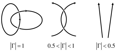
Figure 2: Linking value of two curves for various configurations.

III-B Laplacian Coordinates

Laplacian coordinates [32, 33] describe the spacial relationship of points $p\in\mathbb{R}^{n}$ that are vertices of a graph $G=(V,E)$ relative to their neighborhood points $N_{G}(p)\subseteq V$ in the graph. These coordinates can describe local deformation of the graph but do not represent the relationship of indirectly connected vertices. The Laplacian coordinate $\delta_{i}$ for a point $p_{i}\in V$ is computed by a weighted sum of the neighborhood points,

$$\delta_{i}=p_{i}-\sum_{p_{j}\in N_{G}(p_{i})}\alpha_{ij}p_{j},$$ (3)

where $\alpha_{ij}$ is the normalization weight,

$$\alpha_{ij}=\frac{1}{|p_{j}-p_{i}|\,\sum_{p_{k}\in N_{G}(p_{i})}|p_{k}-p_{i}|^{-1}},$$ (4)

which sums up to 1 for each point $p_{i}$ so that this representation is invariant to scale [23].

III-C Representing the Robot-Humanoid Relationship

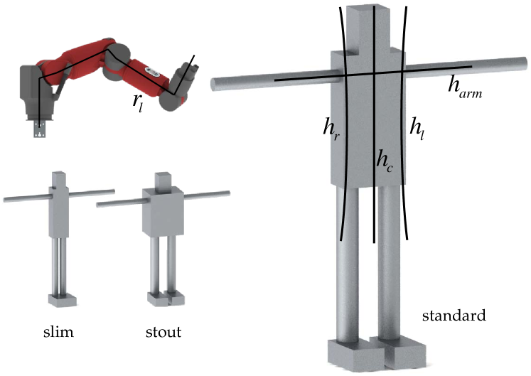
Figure 3: The bodies of robot and humanoid are abstracted to curves. Each robot arm is represented by 7 line segments, and every curve in the humanoid is represented by 10 line segments. We train the policy with the standard model but also test the policy with the slim and stout models.

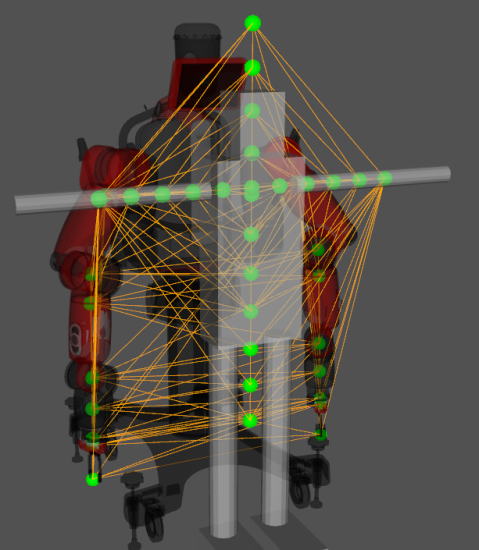
Figure 4: For Laplacian coordinates we construct the graph $G$ from points on the curves in robot’s arms and the humanoid’s body. The orange lines are edges connecting the green vertices.

For our two motion generation scenarios, we combine Writhe matrix and Laplacian coordinates to represent the robot-humanoid relationship, similar to [19, 24]. To this end, we abstract the bodies of the robot and the humanoid into a set of curves consisting of line segments, as seen in Fig. 3. This has the advantage that non-essential features of the bodies’ geometry can be ignored by the learning algorithm.

For the robot

We are only interested in the robot’s arms and ignore all other body parts because only the arms should be used in the interaction. We introduce one curve for the right arm and one curve for the left arm, $r_{\mathrm{r}}$ and $r_{\mathrm{l}}$. Each curve has 7 line segments. The curves run from the base of the arms through the center of the links to the end of the arms where the tool can be attached.

For the humanoid

We want to consider interaction with the arms and the torso. Therefore, we introduce one curve for the arms, $h_{\mathrm{arm}}$, one curve through the neck and the center of the torso, $h_{\mathrm{c}}$, and two curves each running though the shoulder and side of the torso, $h_{\mathrm{r}}$ and $h_{\mathrm{l}}$. Each of the four curves has 10 line segments. The curves $h_{\mathrm{c}}$, $h_{\mathrm{r}}$ and $h_{\mathrm{l}}$ are slightly longer than the torso and the curve $h_{\mathrm{arm}}$ ends approximately at the humanoid’s elbows. For convenience we use superscript notation to refer to the upper and lower half of the curves in the torso as $h_{\mathrm{r}}^{\mathrm{upper}}$ and $h_{\mathrm{r}}^{\mathrm{lower}}$.

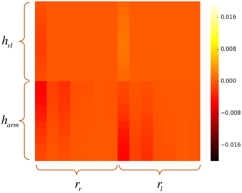
(a) Initial $W_{\mathrm{U}}$

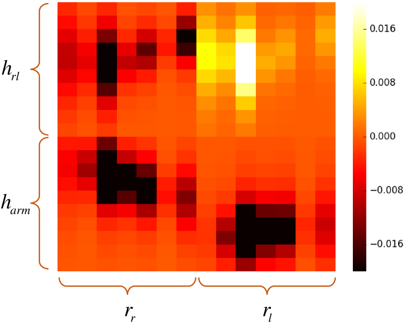
(b) Final $W_{\mathrm{U}}$

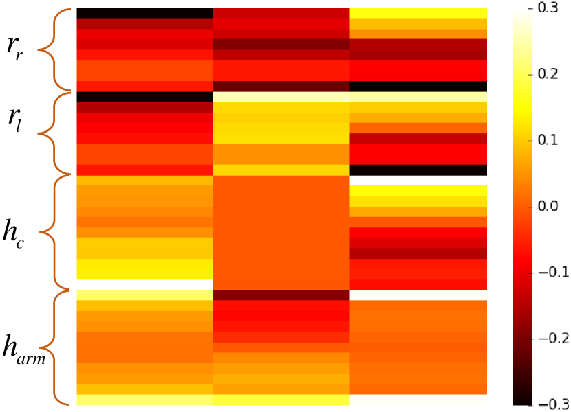
(c) Initial $L_{\mathrm{U}}$

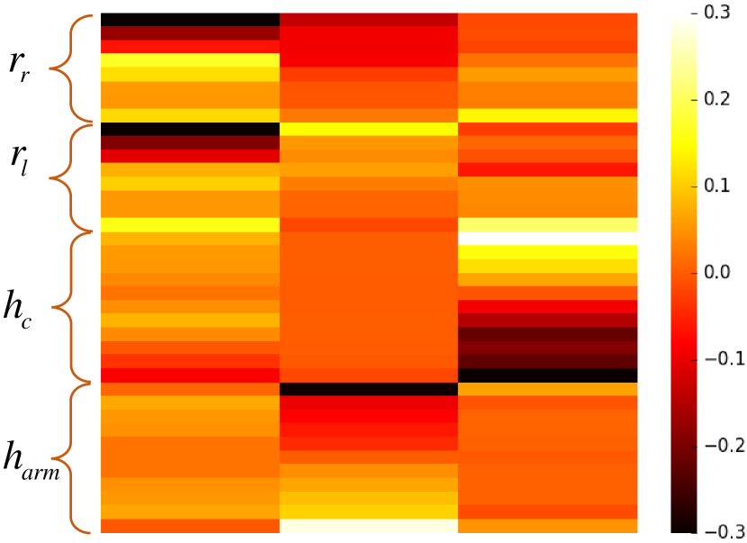
(d) Final $L_{\mathrm{U}}$

Figure 5: The Writhe matrix $W_{\mathrm{U}}$ and the Laplacian coordinates $L_{\mathrm{U}}$ in initial state and final state for the upright scenario. The increase in linking between different body parts is clearly seen in $W_{\mathrm{U}}$.

Based on the curves defined above, we define two representations for interaction with the humanoid. One for the case where the humanoid is upright (see Fig. 1(a)) and one where the humanoid is horizontal (see Fig. 1(b)) in front of the robot. The two cases require different behaviors and using different representations allows better modeling of the relevant relationships. Below, we use the notation $W(\gamma_{1},\gamma_{2})$ for the Writhe matrix of curves $\gamma_{1}$ and $\gamma_{2}$.

Upright Pose

We define one combined Writhe matrix, $W_{\mathrm{U}}\in\mathbb{R}^{20\times 14}$, from the robot’s and humanoid’s curves,

$$W_{\mathrm{U}}=\begin{pmatrix}W(h_{\mathrm{r}},r_{\mathrm{r}})&W(h_{\mathrm{l}},r_{\mathrm{l}})\\ W(h_{\mathrm{arm}},r_{\mathrm{r}})&W(h_{\mathrm{arm}},r_{\mathrm{l}})\end{pmatrix}.$$ (5)

This captures the winding relationship between the robot’s arms and the closest side of the humanoid’s torso as well as the humanoid’s arms. The matrix $W_{\mathrm{U}}$ is visualized in Fig. 5(a)&(b). For the matrix of Laplacian coordinates $L_{\mathrm{U}}\in\mathbb{R}^{38\times 3}$ which captures the spacial relative distance relationship, we define the graph $G=(V,E)$ with 16 vertices from $r_{\mathrm{r}}$ and $r_{\mathrm{l}}$ and 22 vertices from $h_{\mathrm{c}}$ and $h_{\mathrm{arm}}$. The edges $E$ are defined by Delaunay triangulation of $V$ [34]. The graph $G$ is illustrated in Fig. 4 and $L_{\mathrm{U}}$ is visualized in Fig. 5(c)&(d).

Horizontal Pose

We define $W_{\mathrm{H}}\in\mathbb{R}^{15\times 14}$ from the robot’s arm curves and the humanoid’s torso curves,

$$W_{\mathrm{H}}=\begin{pmatrix}W(h_{\mathrm{r}}^{\mathrm{upper}},r_{\mathrm{r}})&W(h_{\mathrm{r}}^{\mathrm{lower}},r_{\mathrm{l}})\\ W(h_{\mathrm{c}}^{\mathrm{upper}},r_{\mathrm{r}})&W(h_{\mathrm{c}}^{\mathrm{lower}},r_{\mathrm{l}})\\ W(h_{\mathrm{l}}^{\mathrm{upper}},r_{\mathrm{r}})&W(h_{\mathrm{l}}^{\mathrm{lower}},r_{\mathrm{l}})\end{pmatrix}.$$ (6)

This captures the winding relationship between the robot’s arms and the upper and lower part of the humanoid’s torso separately. For the matrix $L_{\mathrm{H}}\in\mathbb{R}^{49\times 3}$, we define the graph $G=(V,E)$ with 16 vertices from $r_{\mathrm{r}}$ and $r_{\mathrm{l}}$ and 33 vertices from $h_{\mathrm{c}}$, $h_{\mathrm{l}}$, and $h_{\mathrm{r}}$. The edges $E$ are again defined by Delaunay triangulation of $V$.

IV LEARNING TO GENERATE MOTIONS

We assume that our robot is compliant and has a low-level controller that accepts desired joint angles and drives the robot’s motors while monitoring force and effort limits. That means that our motion policy can command the robot joint angles without directly considering velocities, kinematic, or contacts and we can still get close interaction between the robot and the humanoid. Below we explain how we train the motion policy with deep reinforcement learning. For this, we first define a reinforcement learning problem and model the task with a reward function in Sec. IV-A. In Sec. IV-B we give details about the reinforcement learning algorithm, and in Sec. IV-C we explain the network structure.

IV-A Learning Problem

For setting up a reinforcement learning problem to train the motion generation policy, we need to define a state space $S$, an action space $A$, and a reward function $r_{t}$ for each time step $t$. Below, we first describe the motion that we want to generate in the two interaction scenarios introduced in Sec. III-C, and then formulate the reinforcement learning problem used to learn the policies.

Upright Pose Scenario

The humanoid is positioned upright in front of the robot and we want to achieve a state in which the robot can lift and drag the humanoid backwards, such as in a shoulder drag. To achieve this, we want the robot to move its arms forward and hold the humanoid tightly below the shoulders as seen in Fig. 1(a).

Horizontal Pose Scenario

The humanoid is positioned horizontally in front of the robot and we want to achieve a state in which the robot can lift and carry the humanoid, such as in a cradle lift carry. This is achieved by moving the robot’s arms forward and under the humanoid to hold the humanoid tightly from below as seen in Fig. 1(b).

Action Space and Control

The action space $A=\mathbb{R}^{14}$ is the same in both scenarios and consists of desired changes in joint angles. Therefore, the sum of an action $a\in A$ and the vector of current joint angle $J$ define a new target for the low-level controller, $J+a$. In every time step, the robot has 2 seconds to reach the desired joint angle $J+a$. After that or when the target is reached earlier, the next time step starts.

State Space

In both scenarios, we define the state space $S$ by a combination of the Writhe matrix and the Laplacian coordinates. For the upright case this combination has $20\times 14+38\times 3=394$ dimensions and for the horizontal case it has $15\times 14+49\times 3=357$ dimensions. This state space captures spacial relationships as well as local geometric properties.

Reward Function

For the reward function, we first define the total linking values $\Gamma_{\mathrm{U}}$ and $\Gamma_{\mathrm{H}}$ which sum up the absolute value of linking between the curves that are used to construct the combined Writhe matrices $W_{\mathrm{U}}$ and $W_{\mathrm{H}}$,

$$\Gamma_{\mathrm{U}}= {}|\Gamma(r_{\mathrm{l}},h_{\mathrm{l}})|+|\Gamma(r_{\mathrm{l}},h_{\mathrm{arm}})|+$$

$${}|\Gamma(r_{\mathrm{r}},h_{\mathrm{r}})|+|\Gamma(r_{\mathrm{r}},h_{\mathrm{arm}})|$$ (7)

and

$$\Gamma_{\mathrm{H}}= {}|\Gamma(r_{\mathrm{r}},h_{\mathrm{l}}^{\mathrm{upper}})|+|\Gamma(r_{\mathrm{r}},h_{\mathrm{c}}^{\mathrm{upper}})|+|\Gamma(r_{\mathrm{r}},h_{\mathrm{r}}^{\mathrm{upper}})|+$$

$${}|\Gamma(r_{\mathrm{l}},h_{\mathrm{l}}^{\mathrm{lower}})|+|\Gamma(r_{\mathrm{l}},h_{\mathrm{c}}^{\mathrm{lower}})|+|\Gamma(r_{\mathrm{l}},h_{\mathrm{r}}^{\mathrm{lower}})|.$$ (8)

The total linking values in Eq. (7) and (8) capture the global property of how much the involved curves wind around each other. We select the curves precisely so that these values are maximized in robot-humanoid configurations that are required in our two scenarios. Therefore, we define the reward in terms of total linking value, its recent increment and a punishment term:

$$r_{t}= \beta_{1}\,\left(10\,\Delta_{t}+(\Gamma_{\mathrm{U}})_{t}-\Gamma_{\mathrm{ref}}\right)-$$ (9)

$$\beta_{2}\,(\max(0,z_{\mathrm{r}})+\max(0,z_{\mathrm{l}})).$$

where $\beta_{1},\beta_{2}$ are scale factors, $\Gamma_{\mathrm{ref}}$ is an offset value, and $\Delta_{t}=(\Gamma_{\mathrm{U}})_{t}-(\Gamma_{\mathrm{U}})_{t-1}$ is the last increment in total linking. The second line considers the mean height difference between the robots left and right arm and the humanoid shoulders, $z_{\mathrm{l}}$ and $z_{\mathrm{r}}$, and is 0 when the arms are below the shoulders. This makes sure that the robot holds from below and can actually lift or carry the humanoid with its arms. Eq. (9) is defined analogously for the horizontal scenario.

IV-B Reinforcement Learning

The policy is trained with Proximal Policy Optimization (PPO) [35], which is an actor-critic reinforcement learning method. Actor-critic methods maintain both, a policy estimate (the actor) $\pi(a|s;\theta^{\pi})$, which maps the states to actions, and a value estimate (the critic) $V(s;\theta^{V})$, which predicts the discounted sum of future rewards. Both are modeled as neural networks with their respective parameters $\theta^{\pi}$ and $\theta^{V}$.

During learning, the critic’s loss, $\mathcal{L}_{V}(\theta^{V})$, minimizes the difference between actual return $R_{t}=\sum_{i=t}^{\infty}\gamma^{i-t}r_{i}$ and estimated value, where $\gamma$ is the discount factor. The actor’s objective $\mathcal{J}_{\mathrm{ppo}}(\theta^{\pi})$ maximizes the advantage function, which estimates the difference between the value of output action and all actions. To encourage exploration [36], we add the entropy of the policy, $E(\pi)$, such that the final loss is given by

$$\mathcal{L}=c_{1}\mathcal{L}_{V}(\theta^{V})-\mathcal{J}_{\mathrm{ppo}}(\theta^{\pi})-c_{2}E(\pi(s_{t};\theta^{\pi}))$$ (10)

where $c_{1}$ is the value loss coefficient and $c_{2}$ is the entropy regularization coefficient.

IV-C Network Architecture

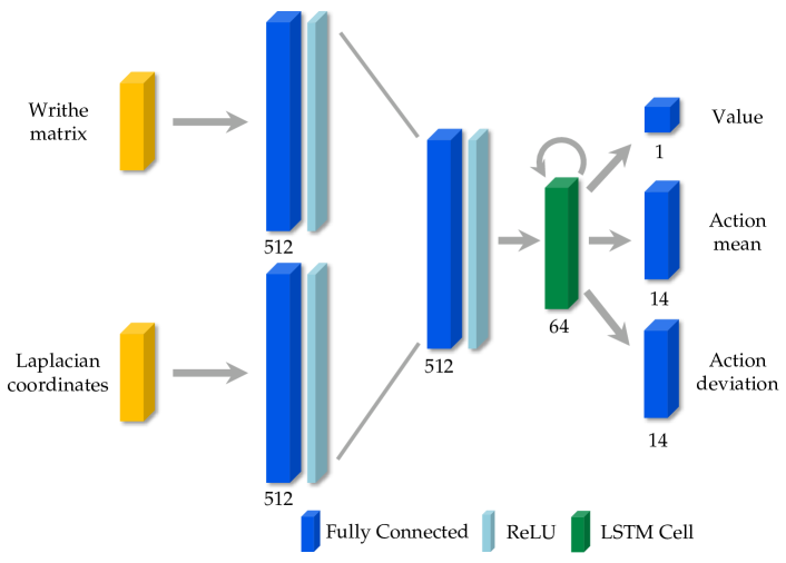
Figure 6: Network structure: The network is composed of a multi-layer perceptron (MLP) base, LSTM unit, and output heads. The inputs are Writhe matrix and Laplacian coordinates and outputs are the scalar value (the critic) and the action vector with its standard deviation (the actor). The fully-connected layers in the base have ReLU activation while action mean and deviation are Tanh and Softplus, respectively.

For reinforcement learning with PPO, we define an actor-critic network as shown in Fig. 6. We feed the Writhe information and the Laplacian coordinates into separate first layers. First two layers extract useful features from the state vector which are then fed into a recurrent neural network. The Long Short-Term Memory (LSTM) [37] unit allows the model to remember previous states. Using three independent layers, the LSTM state is then mapped to the value estimate, the action mean and the action variance, where the last two define the probabilistic policy $\pi$ as a multivariate Gaussian.

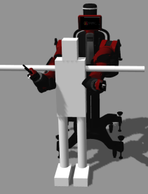
(a) $\Gamma_{\mathrm{U}}=1.5$

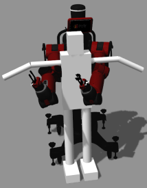
(b) $\Gamma_{\mathrm{U}}=1.7$

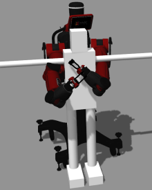
(c) $\Gamma_{\mathrm{U}}=1.9$

(d) $\Gamma_{\mathrm{U}}=2.2$

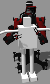
(e) $\Gamma_{\mathrm{U}}=1.6$

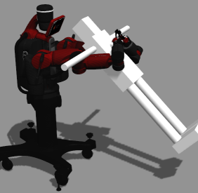
(f) $\Gamma_{\mathrm{U}}=2.1$

Figure 7: Example holding actions executed by Baxter robot in different scenarios. (a-c) Example holdings on the standard humanoid model with the reference linking number $\Gamma_{\mathrm{ref}}=1.5$ and linking number $1.7,1.9$. (d-e) Examples showing holding actions on different humanoid models not involved in training. (f) A holding action applied on a humanoid model floating in water in a non-upright pose. More executions can be found in https://youtu.be/Al-QZl-WGlw.

V EXPERIMENTS

We evaluate our work from $3$ perspectives: 1) we describe the observations in our training process and analyze the network’s performance based on the employed topological and spatial representations, in comparison to using a simple position representation; 2) we quantitatively evaluate the trained policy in terms of the scale of target humanoid model and simulated perception uncertainty; 3) we present qualitative experiments of example application scenarios of the proposed WAM as well as demonstrating a real world example.

The experiments were conducted in Gazebo with a Baxter robot and differently scaled humanoid models and focused on the upright humanoid. In both training and evaluation, we simulate dynamic humanoid models by oscillating the model’s velocity in the vertical direction according to a sinusoidal function with peak-to-peak distance of $25$ cm. For every episode, the humanoid’s model is always initialized with its back facing the robot and we randomize its position within a $40\times 40$ cm² squared region in front of the robot. The step limit $T_{\text{max}}$ for each episode is set to 10 so the total time for one episode is within 20s. Most time is spent on robot movement while the network forward time is only about $0.8$ millisecond.

V-A Network Training

For training the network, we set the parameters as listed in Table I, and used only the standard humanoid model in Fig. 3. For choosing the $\Gamma_{\mathrm{ref}}$ value, we empirically checked a range of reference linking values and decided to set it as $\Gamma_{\mathrm{ref}}=1.5$. As shown in Fig. 7(a), when the total linking number is $1.5$, the robot arms start to form a holding around the humanoid model. In the process of training, we updated the network $4$ times after each episode using the Adam optimizer [38] based on the last $4$ experience batches.

TABLE I: Learning Parameters

Parameter	Notation	Value
Episode limit	$T_{\text{max}}$	10
Reward scale factor	$\beta_{1},\beta_{2}$	$5,1$
Reference Linking	$\Gamma_{\mathrm{ref}}$	1.5
Learning rate	$\eta$	$10^{-4}$
Discount factor	$\gamma$	$0.99$
Value loss coefficient	$c_{1}$	$0.5$
Entropy regularization coefficient	$c_{2}$	$0.01$

In order to evaluate the effectiveness of the proposed representations, we trained the network using $3$ different input spaces: i) as shown in Fig. 6, a network is trained using both the Writhe matrix and the Laplacian coordinates; ii) a network is trained with only the Writhe matrix as the input; and iii) without using the representations developed in this work, we directly use a $3\times 38$ matrix, which contains $38$ position coordinates of the landmark points shown in Fig. 4, as the input to the network for comparison. We repeated the training for each of the $3$ cases for $5$ times and report the average results in Fig. 8.

As seen in Fig. 8(a), when using both the Writhe matrix and Laplacian coordinates, the network was able to converge after experiencing about $600$ episodes and achieved the best result over the $3$ test cases. During the training, to see the performance without exploration deviation noise, we also conducted online evaluation for case i) as shown in Fig. 8(b). For this, we ran the trained policy without variance after every $10$ episodes to try to hold a dynamic humanoid model using $10$ actions, and recorded the resulted total linking number $\Gamma_{\mathrm{U}}$. The result indicates that the network has finally learned how to do this task with a high $\Gamma_{\mathrm{U}}$ value of around $2$. Comparing to the reference $\Gamma_{\mathrm{ref}}=1.5$ and as exemplified in Fig. 7, this will provide robust behaviors to hold the humanoid model.

Figure 8: Training results: (a) The reward mean $r$ of every episode is shown as the training progresses. To filter out the reward noise, each plotted curve is smoothed locally using the $10$ neighboring points. W: Writhe matrix, L: Laplacian coordinates and P: Landmark positions (b) The total linking number $\Gamma_{\mathrm{U}}$ achieved by the configuration (W+L) is evaluated online during training. The number of episode is plotted in log-scale.

In comparison to case i), using only the Writhe matrix to train the network performed worse after the training was converged after $1500$ episodes. This is because of two reasons: firstly, the Writhe matrix by itself does not encode enough relative spatial information between the robot and the humanoid, it is not able to describe geometric interactions. More importantly, by definition different robot states can potentially result in the same Writhe matrix, which can confuse the network in many cases. Lastly, we can see that using only position information of landmark points performed the worst. In our evaluation, it was not able to execute the task even after convergence. This further implies the importance of using the topological representation, which essentially captures the winding interaction between links.

V-B Novel Scenarios and Perception Uncertainty

Having trained the policy using only the standard humanoid model in Fig. 3, we now evaluate its performance using differently shaped and scaled novel models. The trained policy has been applied on some novel humanoid models and a few examples are demonstrated in Fig. 7(d-e). As we can observe, although the humanoid models possess relatively large differences in geometries, the trained policy guided the robot to move its arms around the torso and arms of the humanoid models, and was able to finally achieve holding actions with high linking numbers.

In addition, we quantitatively test the policy by applying it to the $3$ humanoid models in Fig. 3. For each model, we randomize its initial position and keep it moving up and down in front of the robot within a $40\times 40$ cm² region for $100$ times $\times$ $5$ batches and let the network run for $10$ steps for each execution. An execution is successful if the final linking number $\Gamma_{\mathrm{U}}$ is greater than $1.5$. As reported in Table II, the policy performs well and achieves an average success rate of $99\%$ when evaluated with the standard model, which was adopted also in training. For the slim model, the policy performs equally well with a success rate of $98\%$. However, the performance drops to $92.6\%$ for the stout model. As one can observe, the stout model is shorter and wider, which is naturally more difficult to be wrapped around. Moreover, since the robot arms are kept away from each other by the wide torso, the maximum achievable linking number for this model is lower than the others limited by the length of the arms, it is therefore infeasible for the robot to achieve high linking number on it when the model is relatively far from the robot.

TABLE II: Success Rates

Humanoid Model	Success Rate
Standard	$99.00\%\pm 1.10\%$
Slim	$98.00\%\pm 0.89\%$
Stout	$92.60\%\pm 1.96\%$

Figure 9: Evaluation against perception noise $\sigma=0.1,0.2,0.3$m. The average linking number is plotted with its $95\%$ confidence interval for each action step.

For evaluating the system robustness against the perception uncertainty, we simulate the perception errors for the landmark points using Gaussian distributions. In the presence of different magnitudes $\sigma$ of perception errors, we apply the trained policy on the standard humanoid model and recorded the achieved $\Gamma_{\mathrm{U}}$ against the movement step. This experiment is repeated for $100$ times for each $\sigma$ and the statistics is reported in Fig. 9. This result indicates that our trained policy is not significantly affected by the perception noise, since adopted topological representation is not sensitive to the absolute positions of landmark points.

V-C Qualitative Experiments

In addition to holding the upright humanoid models, we applied the learned policy to a fixed floating humanoid as shown in Fig. 7(f). Although the humanoid is spatially different from the upright model, our network was still able to tightly hold the humanoid by winding around the same links. Besides, using the linking $\Gamma_{\mathrm{H}}$ developed in Sec. IV-A, we trained another policy and successfully applied it to hold horizontal humanoid models as demonstrated in Fig. 1(b) and Fig. 10. In addition to the robustness against differently shaped and scaled models, this implies that our formulation of the problem and the developed topological representation are flexible to the orientation of the humanoid model as well.

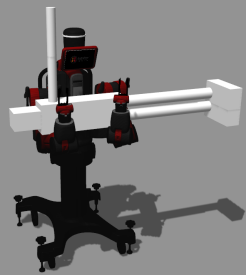
(a) Horizontal slim humanoid

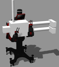
(b) Horizontal stout humanoid

Figure 10: Holding examples for horizontal humanoid case. (a) is with the slim humanoid and (b) is with the stout humanoid.

Moreover, once a holding is achieved, we tried to apply it to two different application cases based on the physical simulation in Gazebo, as shown in Fig. 11. For a standing humanoid, we moved the robot backwards to show that the achieved holding can stably pull the humanoid for transportation. When the humanoid is sitting on the floor, we show that the holding action can safely help it to stand up.

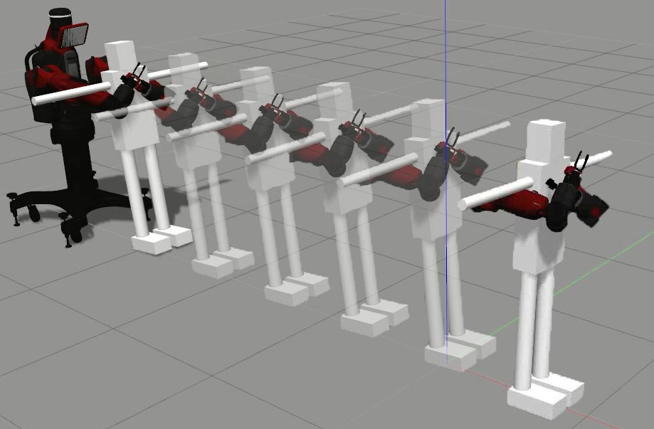
(a) Dragging

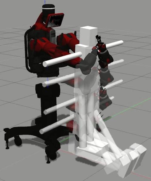
(b) Lifting

Figure 11: Dragging and lifting after holding is achieved.

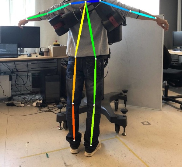
Figure 12: Policy execution in reality: the human is perceived using a depth camera and the skeleton is extracted from the depth data.

Lastly, we applied the policy trained in simulation directly to a real robot as in Fig. 12. The human was successfully held by the robot without requiring any extra tuning. This further shows one of the most important benefits of using topological representations that, since it is insensitive to geometries or perceptions, it can be easily transferred from simulation to reality.

VI CONCLUSION

In this work, we learned a motion policy that enabled WAM of a humanoid with close interaction between the humanoid’s and the robot’s bodies. We used a topology-based representation with Writhe matrix and Laplacian coordinates for reinforcement learning to achieve generalization and reactive behavior in dynamic scenarios. Our results showed that this representation performed better than geometric state encoding in training and achieved a $99\%$ success rate in test. We also demonstrated the robustness and generalization of our policy by applying it in scenarios with unseen, different shape humanoids, floating humanoid, and with perception noise. In the qualitative evaluation, we showed that subsequent transporting was feasible by dragging the humanoid away or lifting it up. Further, we directly applied the policy learned in simulation on a real robot to verify that the policy can be easily transferred to reality.

In future work, we plan to assist the interaction with force sensors mounted on the robot’s arms, in which case the robot would know about physical contacts with the holding targets and the policy would be able to learn a more comfortable way of holding the humanoid.

References

- Bicchi and Kumar [2000] A. Bicchi and V. Kumar, “Robotic grasping and contact: A review,” in ICRA, vol. 348. Citeseer, 2000, p. 353.
- Hang et al. [2017] K. Hang, J. A. Stork, N. S. Pollard, and D. Kragic, “A framework for optimal grasp contact planning,” IEEE Robotics and Automation Letters, vol. 2, no. 2, pp. 704–711, 2017.
- Cosgun et al. [2011] A. Cosgun, T. Hermans, V. Emeli, and M. Stilman, “Push planning for object placement on cluttered table surfaces,” in Proc. IEEE/RSJ Int. Conf. Intelligent Robots and Systems, 2011.
- Haustein et al. [2015] J. A. Haustein, J. King, S. S. Srinivasa, and T. Asfour, “Kinodynamic randomized rearrangement planning via dynamic transitions between statically stable states,” in Proc. IEEE Int. Conf. Robotics and Automation, 2015.
- Yuan et al. [2018] W. Yuan, J. A. Stork, D. Kragic, M. Y. Wang, and K. Hang, “Rearrangement with nonprehensile manipulation using deep reinforcement learning,” arXiv preprint arXiv:1803.05752, 2018.
- Nozawa et al. [2010] S. Nozawa, R. Ueda, Y. Kakiuchi, K. Okada, and M. Inaba, “A full-body motion control method for a humanoid robot based on on-line estimation of the operational force of an object with an unknown weight,” in Intelligent Robots and Systems (IROS), 2010 IEEE/RSJ International Conference on. IEEE, 2010, pp. 2684–2691.
- Florek-Jasińska et al. [2014] M. Florek-Jasińska, T. Wimböck, and C. Ott, “Humanoid compliant whole arm dexterous manipulation: control design and experiments,” in Intelligent Robots and Systems (IROS 2014), 2014 IEEE/RSJ International Conference on. IEEE, 2014, pp. 1616–1621.
- Ohmura and Kuniyoshi [2007] Y. Ohmura and Y. Kuniyoshi, “Humanoid robot which can lift a 30kg box by whole body contact and tactile feedback,” in Intelligent Robots and Systems, 2007. IROS 2007. IEEE/RSJ International Conference on. IEEE, 2007, pp. 1136–1141.
- Onishi et al. [2007] M. Onishi, Z. Luo, T. Odashima, S. Hirano, K. Tahara, and T. Mukai, “Generation of human care behaviors by human-interactive robot ri-man,” in Robotics and Automation, 2007 IEEE International Conference on. IEEE, 2007, pp. 3128–3129.
- Salisbury et al. [1988] K. Salisbury, W. Townsend, B. Ebrman, and D. DiPietro, “Preliminary design of a whole-arm manipulation system (wams),” in Robotics and Automation, 1988. Proceedings., 1988 IEEE International Conference on. IEEE, 1988, pp. 254–260.
- Townsend and Salisbury [1993] W. T. Townsend and J. K. Salisbury, “Mechanical design for whole-arm manipulation,” in Robots and Biological Systems: Towards a New Bionics? Springer, 1993, pp. 153–164.
- Song et al. [2000] P. Song, M. Yashima, and V. Kumar, “Dynamic simulation for grasping and whole arm manipulation,” in Robotics and Automation, 2000. Proceedings. ICRA’00. IEEE International Conference on, vol. 2. IEEE, 2000, pp. 1082–1087.
- Bicchi [1993] A. Bicchi, “Force distribution in multiple whole-limb manipulation,” in Robotics and Automation, 1993. Proceedings., 1993 IEEE International Conference on. IEEE, 1993, pp. 196–201.
- Watanabe et al. [2006] T. Watanabe, K. Harada, T. Yoshikawa, and Z. Jiang, “Towards whole arm manipulation by contact state transition,” in Intelligent Robots and Systems, 2006 IEEE/RSJ International Conference on. IEEE, 2006, pp. 5682–5687.
- Ho et al. [2010a] E. S. Ho, T. Komura, S. Ramamoorthy, and S. Vijayakumar, “Controlling humanoid robots in topology coordinates,” in Intelligent Robots and Systems (IROS), 2010 IEEE/RSJ International Conference on. IEEE, 2010, pp. 178–182.
- Ho and Komura [2011] E. S. Ho and T. Komura, “A finite state machine based on topology coordinates for wrestling games,” Computer Animation and Virtual Worlds, vol. 22, no. 5, pp. 435–443, 2011.
- Stork et al. [2013a] J. A. Stork, F. T. Pokorny, and D. Kragic, “Integrated motion and clasp planning with virtual linking,” in 2013 IEEE/RSJ International Conference on Intelligent Robots and Systems, Nov 2013, pp. 3007–3014.
- Marzinotto et al. [2014] A. Marzinotto, J. A. Stork, D. V. Dimarogonas, and D. Kragic, “Cooperative grasping through topological object representation,” in Humanoid Robots (Humanoids), 2014 14th IEEE-RAS International Conference on. IEEE, 2014, pp. 685–692.
- Ivan et al. [2013] V. Ivan, D. Zarubin, M. Toussaint, T. Komura, and S. Vijayakumar, “Topology-based representations for motion planning and generalization in dynamic environments with interactions,” The International Journal of Robotics Research, vol. 32, no. 9-10, pp. 1151–1163, 2013.
- Kaneko et al. [2000] M. Kaneko, T. Shirai, and T. Tsuji, “Hugging walk,” in Robotics and Automation, 2000. Proceedings. ICRA’00. IEEE International Conference on, vol. 3. IEEE, 2000, pp. 2611–2616.
- Stork et al. [2013b] J. A. Stork, F. T. Pokorny, and D. Kragic, “A topology-based object representation for clasping, latching and hooking,” in Humanoid Robots (Humanoids), 2013 13th IEEE-RAS International Conference on. IEEE, 2013, pp. 138–145.
- Pokorny et al. [2013] F. T. Pokorny, J. A. Stork, D. Kragic et al., “Grasping objects with holes: A topological approach.” in ICRA, 2013, pp. 1100–1107.
- Zarubin et al. [2012] D. Zarubin, V. Ivan, M. Toussaint, T. Komura, and S. Vijayakumar, “Hierarchical motion planning in topological representations,” Proceedings of Robotics: Science and Systems VIII, 2012.
- Ho et al. [2010b] E. S. Ho, T. Komura, and C.-L. Tai, “Spatial relationship preserving character motion adaptation,” in ACM Transactions on Graphics (TOG), vol. 29, no. 4. ACM, 2010, p. 33.
- Mnih et al. [2015] V. Mnih, K. Kavukcuoglu, D. Silver, A. A. Rusu, J. Veness, M. G. Bellemare, A. Graves, M. Riedmiller, A. K. Fidjeland, G. Ostrovski et al., “Human-level control through deep reinforcement learning,” Nature, vol. 518, no. 7540, p. 529, 2015.
- Silver et al. [2017] D. Silver, J. Schrittwieser, K. Simonyan, I. Antonoglou, A. Huang, A. Guez, T. Hubert, L. Baker, M. Lai, A. Bolton et al., “Mastering the game of go without human knowledge,” Nature, vol. 550, no. 7676, p. 354, 2017.
- Lillicrap et al. [2015] T. P. Lillicrap, J. J. Hunt, A. Pritzel, N. Heess, T. Erez, Y. Tassa, D. Silver, and D. Wierstra, “Continuous control with deep reinforcement learning,” arXiv preprint arXiv:1509.02971, 2015.
- Yahya et al. [2017] A. Yahya, A. Li, M. Kalakrishnan, Y. Chebotar, and S. Levine, “Collective robot reinforcement learning with distributed asynchronous guided policy search,” in Intelligent Robots and Systems (IROS), 2017 IEEE/RSJ International Conference on. IEEE, 2017, pp. 79–86.
- Mahler et al. [2017] J. Mahler, J. Liang, S. Niyaz, M. Laskey, R. Doan, X. Liu, J. A. Ojea, and K. Goldberg, “Dex-net 2.0: Deep learning to plan robust grasps with synthetic point clouds and analytic grasp metrics,” arXiv preprint arXiv:1703.09312, 2017.
- OpenAI [2018] OpenAI, “Learning Dexterous In-Hand Manipulation,” arXiv preprint arXiv:1808.00177, 2018.
- Pohl [1968] W. F. Pohl, “The self-linking number of a closed space curve,” Journal of Mathematics and Mechanics, vol. 17, no. 10, pp. 975–985, 1968.
- Chung and Graham [1997] F. R. Chung and F. C. Graham, Spectral graph theory. American Mathematical Soc., 1997, no. 92.
- Zhou et al. [2005] K. Zhou, J. Huang, J. Snyder, X. Liu, H. Bao, B. Guo, and H.-Y. Shum, “Large mesh deformation using the volumetric graph laplacian,” in ACM transactions on graphics (TOG), vol. 24, no. 3. ACM, 2005, pp. 496–503.
- Si and Gärtner [2005] H. Si and K. Gärtner, “Meshing piecewise linear complexes by constrained delaunay tetrahedralizations,” in Proceedings of the 14th international meshing roundtable. Springer, 2005, pp. 147–163.
- Schulman et al. [2017] J. Schulman, F. Wolski, P. Dhariwal, A. Radford, and O. Klimov, “Proximal policy optimization algorithms,” arXiv preprint arXiv:1707.06347, 2017.
- Mnih et al. [2016] V. Mnih, A. P. Badia, M. Mirza, A. Graves, T. Lillicrap, T. Harley, D. Silver, and K. Kavukcuoglu, “Asynchronous methods for deep reinforcement learning,” in International conference on machine learning, 2016, pp. 1928–1937.
- Hochreiter and Schmidhuber [1997] S. Hochreiter and J. Schmidhuber, “Long short-term memory,” Neural computation, vol. 9, no. 8, pp. 1735–1780, 1997.
- Kingma and Ba [2014] D. P. Kingma and J. Ba, “Adam: A method for stochastic optimization,” arXiv preprint arXiv:1412.6980, 2014.