Fourth order finite difference methods for the wave equation with mesh refinement interfaces

Abstract

We analyze two types of summation-by-parts finite difference operators for approximating the second derivative with variable coefficient. The first type uses ghost points, while the second type does not use any ghost points. A previously unexplored relation between the two types of summation-by-parts operators is investigated. By combining them we develop a new fourth order accurate finite difference discretization with hanging nodes on the mesh refinement interface. We take the model problem as the two-dimensional acoustic wave equation in second order form in terms of acoustic pressure, and prove energy stability for the proposed method. Compared to previous approaches using ghost points, the proposed method leads to a smaller system of linear equations that needs to be solved for the ghost point values. Another attractive feature of the proposed method is that the explicit time step does not need to be reduced relative to the corresponding periodic problem. Numerical experiments, both for smoothly varying and discontinuous material properties, demonstrate that the proposed method converges to fourth order accuracy. A detailed comparison of the accuracy and the time-step restriction with the simultaneous-approximation-term penalty method is also presented.

1 Introduction

Based on the pioneering work by Kreiss and Oliger [12], it is by now well known that high order accurate ($\geq 4$) numerical methods for solving hyperbolic partial differential equations (PDE) are more efficient than low order methods. While Taylor series expansion can easily be used to construct high order finite difference stencils for the interior of the computational domain, it is in general difficult to find stable boundary closures that avoid spurious growth in time of the numerical solution. Finite difference operators that satisfy the summation-by-parts (SBP) identity, first introduced by Kreiss and Scherer [14], provide a recipe for achieving both stability and high order accuracy.

An SBP operator is constructed such that the energy estimate of the continuous PDE can be carried out discretely for the finite difference approximation, with summation-by-parts replacing the integration-by-parts principle. As a consequence, a discrete energy estimate can be obtained to ensure that the discretization is energy stable. When deriving a continuous energy estimate, the boundary terms resulting from the integration-by-parts formula are easily controlled through the boundary conditions. The fundamental benefit of using SBP operators is that a discrete energy estimate can be derived in a similar way. Here, the summation-by-parts identities result in discrete boundary terms. These terms dictate how the boundary conditions must be discretized to guarantee energy stability for the finite difference approximation.

We consider the SBP discretization of the two-dimensional acoustic wave equation on Cartesian grids, and focus on the case when the material properties are discontinuous in a semi-infinite domain. To obtain high order accuracy, one approach is to decompose the domain into multiple subdomains, such that the material is smooth within each subdomain. The governing equation is then discretized by SBP operators in each subdomain, and patched together by imposing interface conditions at the material discontinuity. For computational efficiency, the mesh size in each subdomain should be chosen inversely proportional to the wave speed [9, 14], leading to mesh refinement interfaces with hanging nodes.

We develop two approaches for imposing interface conditions in the SBP finite difference framework. In the first approach, interface conditions are imposed strongly by using ghost points. In this case, the SBP operators also utilize ghost points in the difference approximation. We call this the SBP-GP method. In the second approach, the SBP-SAT method, interface conditions are imposed weakly by adding penalty terms, also known as simultaneous-approximation-terms (SAT) [3]. The addition of penalty terms in the SBP-SAT method bears similarities with the discontinuous Galerkin method [10]. A high order accurate SBP-SAT discretization of the acoustic wave equation in second order form was previously developed by Wang et al. [31]. Petersson and Sjögreen [22] developed a second order accurate SBP-GP scheme for the elastic wave equation in displacement formulation with mesh refinement interfaces. We note that the projection method [20, 21] could in principle also be used to impose interface conditions, but will not be considered here.

In this paper, we present two ways of generalizing the SBP-GP method in [22] to fourth order accuracy. The first approach is a direct generalization of the second order accurate technique. It imposes the interface conditions using ghost points from both sides of the mesh refinement interface. The second approach is based on a previously unexplored relation between SBP operators with and without ghost points. This relation allows for an improved version of the fourth order SBP-GP method, where only ghost points from one side of the interface are used to impose the interface conditions. This approach reduces the computational cost of updating the solution at the ghost points and should also simplify the generalization to three-dimensional problems.

Even though both the SBP-GP and SBP-SAT methods have been used to solve many kinds of PDEs, the relation between them has previously not been explored. An additional contribution of this paper is to connect the two approaches, provide insights into their similarities and differences, as well as making a comparison in terms of their efficiency.

The remainder of the paper is organized as follows. In Section 2, we introduce the SBP methodology and present the close relation between the SBP operators with and without ghost points. In Section 3, we derive a discrete energy estimate for the wave equation in one space dimension with Dirichlet or Neumann boundary conditions. Both the SBP-GP and the SBP-SAT methods are analyzed in detail and their connections are discussed. In Section 4, we consider the wave equation in two space dimensions, and focus on the numerical treatment of grid refinement interfaces with the SBP-GP and SBP-SAT methods. Numerical experiments are conducted in Section 5, where we compare the SBP-GP and SBP-SAT methods in terms of their time-step stability condition and solution accuracy. Our findings are summarized in Section 6.

2 SBP operators

Consider the bounded one-dimensional domain $x\in[0,1]=:\Omega$ and the uniform grid on $\Omega$,

$$\boldsymbol{x}=[x_{1},\cdots,x_{n}]^{T},\quad x_{j}=(j-1)h,\quad j=1,2,\cdots,n,\quad h=1/(n-1).$$

The grid points in $\boldsymbol{x}$ are either in the interior of $\Omega$, or on its boundary. We also define two ghost points outside of $\Omega$: $x_{0}=-h$ and $x_{n+1}=1+h$. Let the vector $\widetilde{\boldsymbol{x}}=[x_{0},\cdots,x_{n+1}]^{T}$ denote the grid with ghost points. Throughout this paper, we will use the tilde symbol to indicate that ghost points are involved in a grid, a grid function, or in a difference operator.

We consider a smooth function $u(x)$ in the domain $\Omega$, and define the grid function $u_{j}:=u(x_{j})$. Let

$$\boldsymbol{u}=[u_{1},\cdots,u_{n}]^{T}\text{ and }\boldsymbol{v}=[v_{1},\cdots,v_{n}]^{T}$$ (1)

denote real-valued grid functions on $\boldsymbol{x}$, and let

$$\widetilde{\boldsymbol{u}}=[u_{0},\boldsymbol{u}^{T},u_{n+1}]^{T}\text{ and }\widetilde{\boldsymbol{v}}=[v_{0},\boldsymbol{v}^{T},v_{n+1}]^{T}$$ (2)

denote the corresponding real-valued grid functions on $\widetilde{\boldsymbol{x}}$.

We denote the standard discrete $L^{2}$ inner product by

$$({\boldsymbol{u}},{\boldsymbol{v}})_{2}=h\sum_{j=1}^{n}u_{j}v_{j}.$$

For SBP operators, we need the weighted inner product

$$({\boldsymbol{u}},{\boldsymbol{v}})_{h}=h\sum_{j=1}^{n}w_{j}u_{j}v_{j},\quad w_{j}\geq\delta>0,$$ (3)

where $\delta$ is a constant, $w_{j}=1$ in the interior of the domain and $w_{j}\neq 1$ at a few grid points near each boundary. The number of grid points with $w_{j}\neq 1$ is independent of $n$, but depends on the order of accuracy of the SBP operator. Let $\|\cdot\|_{h}$ be the SBP norm induced from the inner product $(\cdot,\cdot)_{h}$. Furthermore, let the diagonal matrix $W$ have entries $W_{jj}=hw_{j}>0$. Then, in matrix-vector notation, $(\boldsymbol{u},\boldsymbol{v})_{h}=\boldsymbol{u}^{T}W\boldsymbol{v}$.

The SBP methodology was introduced by Kreiss and Scherer in [14], where the first derivative SBP operator $D\approx\partial/\partial x$ was also constructed. The operator $D$ does not use ghost points, and satisfies the first derivative SBP identity.

Definition 1 (First derivative SBP identity).

The difference operator $D$ is a first derivative SBP operator if it satisfies

$$({\boldsymbol{u}},D{\boldsymbol{v}})_{h}=-(D{\boldsymbol{u}},{\boldsymbol{v}})_{h}-u_{1}v_{1}+u_{n}v_{n},$$ (4)

for all grid functions $\boldsymbol{u}$ and $\boldsymbol{v}$.

We note that (4) is a discrete analogue of the integration-by-parts formula

$$\int_{0}^{1}u\frac{dv}{dx}dx=-\int_{0}^{1}\frac{du}{dx}v-u(0)v(0)+u(1)v(1).$$

Centered finite difference stencils are used on the grid points away from the boundaries, where the weights in the SBP norm are equal to one. To retain the SBP identity, special one-sided boundary stencils must be employed at a few grid points near each boundary. Kreiss and Scherer showed in [14] that the order of accuracy of the boundary stencil must be lower than in the interior stencil. With a diagonal norm and a $2p^{th}$ order accurate interior stencil, the boundary stencil can be at most $p^{th}$ order accurate. The overall convergence rate can be between $p+1/2$ and $2p$, depending on the equation and the numerical treatment of boundary and interface conditions [8, 29, 30]. In the following we refer to the accuracy of an SBP operator by its interior order of accuracy ($2p$).

It is possible to construct block norm SBP operators with $2p^{th}$ order interior stencils and $(2p-1)^{th}$ order boundary stencils. Despite their superior accuracy, the block norm SBP operators are seldomly used in practice because of stability issues related to variable coefficients. However, in some cases the block norm SBP operators can be stabilized using artificial dissipation [16].

For second derivative SBP operators, we focus our discussion on discretizing the expression

$$\frac{d}{dx}\left(\mu(x)\frac{dv}{dx}(x)\right).$$ (5)

Here, the smooth function $\mu(x)>0$ may represent a variable material property or a metric coefficient. In the following we introduce two different types of second derivative SBP operators that are based on a diagonal norm. The first type uses one ghost point outside each boundary, while the second type does not use any ghost points. We proceed by explaining the close relation between these operators. To make the presentation concise, we exemplify the relation for the case of fourth order accuracy ($2p=4)$.

2.1 Second derivative SBP operators with ghost points

Sjögreen and Petersson [26] derived a fourth order accurate SBP discretization $\widetilde{G}(\mu)\widetilde{\boldsymbol{v}}$ for approximating (5). This discretization was originally developed for solving the seismic wave equations and is extensively used in the software package SW4 [24]. The formula is based on a five-point centered difference stencil of fourth order accuracy in the interior of the domain. Special one-sided boundary stencils of second order accuracy are used at the first six grid points near each boundary. Note, in particular, that $\widetilde{G}(\mu)\widetilde{\boldsymbol{v}}$ uses the ghost point values of $\widetilde{\boldsymbol{u}}$ to approximate (5) on the boundary itself, as illustrated in Figure 1.

Figure 1: The non-zero coefficients of the SBP operator $\widetilde{G}(\mu)$ in matrix form, for a grid with 30 grid points. Blue circles: standard five-point difference stencil. Red triangles: special boundary stencil. Black squares: ghost points. The structure of $G(\mu)$ is the same, but without the black squares. Note that the grid function $\widetilde{G}(\mu)\widetilde{\boldsymbol{v}}$ is defined at the same grid points as $\boldsymbol{v}$.

As will be shown below, the difference approximation of the wave equation is energy stable because the difference operator $\widetilde{G}(\mu)$ satisfies the second derivative SBP identity.

Definition 2 (Second derivative SBP identity).

The difference operator $\widetilde{G}(\mu)$ is a second derivative SBP operator if it satisfies

$$(\boldsymbol{u},\widetilde{G}(\mu)\widetilde{\boldsymbol{v}})_{h}=-S_{\mu}(\boldsymbol{u},\boldsymbol{v})-u_{1}\mu_{1}\widetilde{\boldsymbol{b}}_{1}^{T}\widetilde{\boldsymbol{v}}+u_{n}\mu_{n}\widetilde{\boldsymbol{b}}_{n}^{T}\widetilde{\boldsymbol{v}},$$ (6)

for all grid functions $\boldsymbol{u}$ and $\widetilde{\boldsymbol{v}}$. Here, $\mu_{1}=\mu(x_{1})$, $\mu_{n}=\mu(x_{n})$ and the bilinear form $S_{\mu}(\cdot,\cdot)$ is symmetric and positive semi-definite. The boundary difference formulas $\widetilde{\boldsymbol{b}}_{1}^{T}\widetilde{\boldsymbol{v}}$ and $\widetilde{\boldsymbol{b}}_{n}^{T}\widetilde{\boldsymbol{v}}$ approximate $dv/dx$ at $x_{1}$ and $x_{n}$, making use of the ghost point values $v_{0}$ and $v_{n+1}$, respectively.

We remark that the boundary difference operators, $\widetilde{\boldsymbol{b}}_{1}^{T}$ and $\widetilde{\boldsymbol{b}}_{n}^{T}$, are constructed with fourth order accuracy in [26]. Note that (6) is a discrete analogue of the integration-by-parts formula

$$\int_{0}^{1}u\frac{d}{dx}\left(\mu\frac{dv}{dx}\right)dx=-\int_{0}^{1}\mu\frac{du}{dx}\frac{dv}{dx}-u(0)\mu(0)\frac{dv}{dx}(0)+u(1)\mu(1)\frac{dv}{dx}(1).$$

2.2 Second derivative SBP operators without ghost points

The second type of second derivative SBP operator, denoted by $G_{2p}(\mu)$, does not use any ghost points. This type of operator was constructed by Mattsson [15] for the cases of second, fourth and sixth order accuracy ($2p=2,4,6$). In the following discussion we focus on the fourth order case and define $G(\mu)=G_{4}(\mu)$.

In the interior of the domain, the operator $G(\mu)$ uses the same five-point wide, fourth order accurate stencil as the operator with ghost points, $\widetilde{G}(\mu)$. At the first six grid points near the boundaries, the two operators are similar in that they both use a second order accurate one-sided difference stencil that satisfies an SBP identity of the form (6), but without ghost points,

$$({\boldsymbol{u}},G(\mu){\boldsymbol{v}})_{h}=-S_{\mu}({\boldsymbol{u}},{\boldsymbol{v}})_{h}-u_{1}\mu_{1}{\boldsymbol{b}}_{1}^{T}{\boldsymbol{v}}+u_{n}\mu_{n}{\boldsymbol{b}}_{n}^{T}{\boldsymbol{v}}.$$ (7)

Similar to (6), the bilinear form $S_{\mu}(\cdot,\cdot)$ is symmetric and positive semi-definite. In this case, the boundary difference operators ${\boldsymbol{b}}_{1}^{T}$ and ${\boldsymbol{b}}_{n}^{T}$ are constructed with third order accuracy, using stencils that do not use any ghost points. The structure of $G(\mu)$ is the same as shown in Figure 1, but without the two black squares representing the ghost points.

2.3 The relation between SBP operators with and without ghost points

When using the SBP operator $\widetilde{G}(\mu)$ with ghost points, boundary conditions are imposed in a strong sense by using the ghost point values as additional degrees of freedom. On the other hand, for the SBP operator $G(\mu)$ without ghost points, boundary conditions are imposed weakly by using a penalty technique. Though these two types of SBP operators are used in different ways, they are closely related to each other. In fact, an SBP operator with ghost points can easily be modified into a new SBP operator that does not use any ghost points, and vice versa. The new operators preserve the SBP identity and the order of accuracy of the original operators. In the following, we demonstrate this procedure for the fourth order accurate version of $\widetilde{G}(\mu)$ [26] and $G(\mu)$ [15]. For simplicity, we only consider the stencils near the left boundary. The stencils near the right boundary can be treated in a similar way.

To discuss accuracy, let us assume that the grid function $\widetilde{\boldsymbol{v}}$ is a restriction of a sufficiently smooth function $V(x)$ on the grid $\widetilde{\boldsymbol{x}}$. The boundary difference operator associated with $\widetilde{G}(\mu)$ satisfies

$$\widetilde{\boldsymbol{b}}_{1}^{T}\widetilde{\boldsymbol{v}}=\frac{1}{12h}(-3v_{0}-10v_{1}+18v_{2}-6v_{3}+v_{4})=\frac{dV}{dx}(x_{1})+\mathcal{O}(h^{4}).$$ (8)

Let’s consider the modified boundary difference operator,

$$\widetilde{\boldsymbol{b}}_{1}^{T}\widetilde{\boldsymbol{v}}+\beta h^{4}\widetilde{\boldsymbol{d}}^{T}_{5+}\widetilde{\boldsymbol{v}},$$ (9)

where

$$\widetilde{\boldsymbol{d}}^{T}_{5+}\widetilde{\boldsymbol{v}}=\frac{1}{h^{5}}(-v_{0}+5v_{1}-10v_{2}+10v_{3}-5v_{4}+v_{5})=\frac{d^{5}V}{dx^{5}}(x_{1})+\mathcal{O}(h)$$ (10)

is a first order accurate approximation of the fifth derivative at the boundary point $x_{1}$. Both the approximations (8) and (9) are exact at $x_{1}$ if $V(x)$ is a polynomial of order at most four. For any (finite) value of $\beta$, (9) is a fourth order accurate approximation of $\frac{dV}{dx}(x_{1})$.

We note that the coefficient of $v_{0}$ in (8) is -1/4. To eliminate the dependence on $v_{0}$ in (9), we choose $\beta=-1/4$ and define a new boundary difference operator by

$$\widetilde{\underline{\boldsymbol{b}}}_{1}^{T}\boldsymbol{v}=\frac{1}{12h}(-25v_{1}+48v_{2}-36v_{3}+16v_{4}-3v_{5})=V_{x}(x_{1})+\mathcal{O}(h^{4}).$$

This stencil does not use the ghost point value $v_{0}$. Instead, it uses the value $v_{5}$, which is not used by $\widetilde{\boldsymbol{b}}_{1}^{T}\widetilde{\boldsymbol{v}}$. Here and throughout the paper, we use an underbar to indicate operators that have been modified by adding/removing ghost points.

To retain the SBP identity (6), the operator $\widetilde{G}(\mu)$ must be changed accordingly. We can maintain the same bilinear form $S_{\mu}(\cdot,\cdot)$ if we only modify $\widetilde{G}(\mu)$ on the boundary itself. We make the ansatz

$$\underline{\widetilde{G}}_{1}(\mu)\boldsymbol{v}=\widetilde{G}_{1}(\mu)\widetilde{\boldsymbol{v}}+\widetilde{\boldsymbol{a}}^{T}\widetilde{\boldsymbol{v}},$$ (11)

where $\widetilde{G}_{1}(\mu)\widetilde{\boldsymbol{v}}$ should be interpreted as the first element of vector $\widetilde{G}(\mu)\widetilde{\boldsymbol{v}}$. To see the relation between $\underline{\widetilde{G}}_{1}(\mu)\boldsymbol{v}$ and $\widetilde{G}_{1}(\mu)\widetilde{\boldsymbol{v}}$ in the SBP identity (6), we pick a particular grid function $\boldsymbol{u}$ in (6) satisfying $u_{1}=1$ and $u_{j}=0$, for $j\geq 2$. The balance between the left and right hand sides of that equation is maintained if

$$hw_{1}\widetilde{\boldsymbol{a}}^{T}\widetilde{\boldsymbol{v}}=-\beta h^{4}\mu_{1}\widetilde{\boldsymbol{d}}^{T}_{5+}\widetilde{\boldsymbol{v}}\quad\Rightarrow\quad\widetilde{\boldsymbol{a}}^{T}\widetilde{\boldsymbol{v}}=\frac{12}{17}h^{3}\mu_{1}\widetilde{\boldsymbol{d}}^{T}_{5+}\widetilde{\boldsymbol{v}}.$$

Here we have used that $\beta=-1/4$ and that $w_{1}=17/48$ is the weight of the SBP norm at the first grid point. The ghost point value $v_{0}$ is only used by $\widetilde{G}(\mu)\widetilde{\boldsymbol{v}}$ on the boundary itself. It satisfies

$$\widetilde{G}_{1}(\mu)\widetilde{\boldsymbol{v}}=\frac{1}{h^{2}}\sum_{k=1}^{8}\sum_{m=1}^{8}\beta_{k,m}\mu_{m}v_{k}+\frac{12}{17}\frac{\mu_{1}}{h^{2}}v_{0},$$ (12)

where $\beta_{k,m}$ are constants [26] (the numerical values can be found in the open source code of SW4 [24]). Because the coefficient of $v_{0}$ in $\widetilde{\boldsymbol{d}}^{T}_{5+}\widetilde{\boldsymbol{v}}$ is $-1/h^{5}$, the dependence on $v_{0}$ cancels in (11). This cancellation is a consequence of the operators $\widetilde{G}(\mu)$ using ghost points only from $\widetilde{\boldsymbol{b}}_{1}^{T}$ but not $S_{\mu}(\cdot,\cdot)$, see [26] for details.

The new SBP difference operator that does not use ghost points can be written as

$$\underline{\widetilde{G}}_{1}(\mu)\boldsymbol{v} =\frac{1}{h^{2}}\sum_{k=1}^{8}\sum_{m=1}^{8}\beta_{k,m}\mu_{m}v_{k}+\frac{12}{17}\frac{\mu_{1}}{h^{2}}\left(5v_{1}-10v_{2}+10v_{3}-5v_{4}+v_{5}\right),$$

$$\underline{\widetilde{G}}_{j}(\mu)\boldsymbol{v} =\widetilde{G}_{j}(\mu)\widetilde{\boldsymbol{v}},\quad j=2,3,\ldots.$$

Note that the second equation is satisfied independently of the ghost point value, $v_{0}$.

To emphasize that $\widetilde{\underline{G}}(\mu)$ is modified from $\widetilde{G}(\mu)$, we keep the tilde symbol on $\widetilde{\underline{G}}(\mu)$, even though the operator does not use any ghost points. The new operator pair $(\underline{\widetilde{G}}(\mu),\underline{\widetilde{\boldsymbol{b}}}_{1})$ shares important properties with the original operator pair $(\widetilde{G}(\mu),{\widetilde{\boldsymbol{b}}}_{1})$. In particular, both pairs satisfy the SBP identity 2 and have the same orders of accuracy in the interior and near each boundary. Even though the SBP operator $\widetilde{\underline{G}}(\mu)$ does not use any ghost points, it is not the same as the SBP operator $G(\mu)$ constructed by Mattssson [15]. The dissimilarity arises because the corresponding boundary difference operators are constructed with different orders of accuracy.

For the SBP operator pair $(G(\mu),\boldsymbol{b}_{1})$ that does not use ghost points, we can reverse the above procedure to derive a new pair of SBP operator that uses a ghost point. The boundary difference operator associated with ${G}(\mu)$ is

$$\boldsymbol{b}_{1}^{T}\boldsymbol{v}=\frac{1}{6h}(-11v_{1}+18v_{2}-9v_{3}+2v_{4})=\frac{dV}{dx}(x_{1})+\mathcal{O}(h^{3}).$$ (13)

Another third order approximation of $dV/dx(x_{1})$ is given by the difference formula

$${\boldsymbol{b}}_{1}^{T}{\boldsymbol{v}}+\gamma h^{3}\widetilde{\boldsymbol{d}}_{4+}^{T}\widetilde{\boldsymbol{v}},$$ (14)

where

$$\widetilde{\boldsymbol{d}}_{4+}^{T}\widetilde{\boldsymbol{v}}=\frac{1}{h^{4}}(v_{0}-4v_{1}+6v_{2}-4v_{3}+v_{4})=\frac{d^{4}V}{dx^{4}}(x_{1})+\mathcal{O}(h).$$ (15)

The boundary operator (13) is exact for any polynomial $V(x)$ of order at most three and $\widetilde{\boldsymbol{d}}_{4+}^{T}\widetilde{\boldsymbol{v}}=0$ for such polynomials. Therefore, (14) is third order accurate for any value of $\gamma$. By choosing $\gamma=-1/3$, we obtain a new boundary difference operator that uses the ghost point value $v_{0}$, but does not depend on $v_{4}$,

$$\underline{\boldsymbol{b}}_{1}^{T}\widetilde{\boldsymbol{v}}:=\boldsymbol{b}_{1}^{T}\boldsymbol{v}-\frac{1}{3}h^{3}\widetilde{\boldsymbol{d}}_{4+}^{T}\widetilde{\boldsymbol{v}}=\frac{1}{6h}(-2v_{0}-3v_{1}+6v_{2}-v_{3})=\frac{dV}{dx}(x_{1})+\mathcal{O}(h^{3}).$$ (16)

As a result, the new boundary difference operator has the minimum stencil width for a third order accurate approximation of a first derivative.

To satisfy the SBP identity (6) for difference operators that include ghost points, we must modify $G(\mu)$ to be compatible with the new boundary difference operator $\underline{\boldsymbol{b}}^{T}_{1}$. As before, we consider a grid function $\boldsymbol{u}$ with $u_{1}=1$ and $u_{j}=0$, for $j\geq 2$. To maintain the balance between the left and right hand sides of (6), the following must hold

$$\underline{G}_{1}(\mu)\widetilde{\boldsymbol{v}}:=G_{1}(\mu)\boldsymbol{v}-\frac{\gamma h^{3}}{w_{1}h}\mu_{1}\widetilde{\boldsymbol{d}}_{4+}^{T}\widetilde{\boldsymbol{v}}=G_{1}(\mu)\boldsymbol{v}+\frac{16}{17}h^{2}\mu_{1}\widetilde{\boldsymbol{d}}_{4+}^{T}\widetilde{\boldsymbol{v}}.$$ (17)

The new SBP operator that uses a ghost point becomes

$$\underline{G}_{j}(\mu)\widetilde{\boldsymbol{v}}=\begin{cases}G_{1}(\mu)\boldsymbol{v}+\frac{16}{17}h^{2}\mu_{1}\widetilde{\boldsymbol{d}}_{4+}^{T}\widetilde{\boldsymbol{v}},\quad&j=1,\\ G_{j}(\mu)\boldsymbol{v},\quad&j=2,3,4,\ldots.\end{cases}$$

Even though the new difference operators use a ghost point, we have not added tilde symbols on $(\underline{G}(\mu),\underline{\boldsymbol{b}}_{1})$. This is to emphasize that they are modified from the operators without ghost points, $(G(\mu),\boldsymbol{b}_{1})$.

3 Boundary conditions

To present the techniques for imposing boundary conditions with and without ghost points, and to highlight the relation between the SBP-GP and SBP-SAT approaches, we consider the one-dimensional wave equation,

$$\rho U_{tt}=(\mu(x)U_{x})_{x},\quad x\in[0,1],\ t\geq 0,$$ (18)

subject to smooth initial conditions. Here, $\rho(x)>0$ and $\mu(x)>0$ are material parameters. The dependent variable $U(x,t)$ could, for example, represent the acoustic overpressure in a linearized model of a compressible fluid. $U_{tt}$ is the second derivative with respect to time and the subscript $x$ denotes differentiation with respect to the spatial variable.

We have for simplicity not included a forcing function in the right-hand side of (18). This is because it has no influence on how boundary conditions are imposed. We only consider imposing the boundary condition on the left boundary, $x=0$. Consequently, boundary terms corresponding to the right boundary are omitted from the description below. Furthermore, the initial conditions are assumed to be compatible with the boundary conditions.

3.1 Neumann boundary conditions

We start by considering the Neumann boundary condition

$$U_{x}(0,t)=f(t),\quad t\geq 0.$$ (19)

In the SBP-GP method, the semi-discretization of (18)-(19) is

$$\boldsymbol{\rho}{\boldsymbol{u}}_{tt} =\widetilde{G}(\mu)\widetilde{\boldsymbol{u}},\quad t\geq 0,$$ (20)

$$\widetilde{\boldsymbol{b}}_{1}^{T}\widetilde{\boldsymbol{u}} =f(t),\quad t\geq 0,$$ (21)

where $\boldsymbol{\rho}$ is a diagonal matrix with the $j^{th}$ diagonal element $\rho_{j}=\rho(x_{j})$, $\widetilde{\boldsymbol{u}}=\widetilde{\boldsymbol{u}}(t)$ is a time-dependent grid function on $\widetilde{\boldsymbol{x}}$ and $\boldsymbol{u}=\boldsymbol{u}(t)$ is the corresponding grid function on $\boldsymbol{x}$. By using the SBP identity (6), we obtain

$$\begin{split}\left(\boldsymbol{u}_{t},\boldsymbol{\rho}\boldsymbol{u}_{tt}\right)_{h}&=\left(\boldsymbol{u}_{t},\widetilde{G}(\mu)\widetilde{\boldsymbol{u}}\right)_{h}\\ &=-S_{\mu}(\boldsymbol{u}_{t},\boldsymbol{u})-(u_{1})_{t}\mu_{1}\widetilde{\boldsymbol{b}}_{1}^{T}\widetilde{\boldsymbol{u}},\end{split}$$

which can be written as,

$$\left(\boldsymbol{u}_{t},\boldsymbol{\rho}\boldsymbol{u}_{tt}\right)_{h}+S_{\mu}(\boldsymbol{u}_{t},\boldsymbol{u})=-(u_{1})_{t}\mu_{1}\widetilde{\boldsymbol{b}}_{1}^{T}\widetilde{\boldsymbol{u}}.$$ (22)

We define the discrete energy

$$E_{h}:=(\boldsymbol{u}_{t},\boldsymbol{\rho}\boldsymbol{u}_{t})_{h}+S_{\mu}(\boldsymbol{u},\boldsymbol{u}),$$

and note that the left-hand side of equation (22) equals the change rate of the discrete energy,

$$\frac{d}{dt}E_{h}=-2(u_{1})_{t}\mu_{1}\widetilde{\boldsymbol{b}}_{1}^{T}\widetilde{\boldsymbol{u}}.$$ (23)

To obtain energy stability, we need to impose the Neumann boundary condition such that the right-hand side of (23) is non-positive when $f=0$. The key in the SBP-GP method is to use the ghost point as the additional degree of freedom for imposing the boundary condition. Here, the Neumann boundary condition (19) is approximated by enforcing $\widetilde{\boldsymbol{b}}_{1}^{T}\widetilde{\boldsymbol{u}}(t)=f(t)$. From (8), it is satisfied if

$$u_{0}=\frac{1}{3}(-10u_{1}+18u_{2}-6u_{3}+u_{4}-12hf(t)),\quad t\geq 0.$$ (24)

This relation gives the ghost point value $u_{0}$ as function of the interior values $u_{j}$, $j=1,2,3,4$. The resulting approximation is energy conservative because

$$\frac{d}{dt}E_{h}=0,\quad f(t)=0.$$ (25)

Next, consider the semi-discretization of (18) by the SBP-SAT method in [15],

$$\boldsymbol{\rho}\boldsymbol{u}_{tt}=G(\mu)\boldsymbol{u}+\boldsymbol{p}_{N},$$ (26)

where $\boldsymbol{p}_{N}$ is a penalty term for enforcing the Neumann condition (19). By using the SBP identity (7), we obtain

$$\begin{split}(\boldsymbol{u}_{t},\boldsymbol{\rho}\boldsymbol{u}_{tt})_{h}&=(\boldsymbol{u}_{t},G(\mu)\boldsymbol{u})_{h}+(\boldsymbol{u}_{t},\boldsymbol{p}_{N})_{h}\\ &=-S_{\mu}(\boldsymbol{u}_{t},\boldsymbol{u})-(u_{1})_{t}\mu_{1}\boldsymbol{b}_{1}^{T}\boldsymbol{u}+(\boldsymbol{u}_{t},\boldsymbol{p}_{N})_{h},\end{split}$$

which can be written as

$$\frac{d}{dt}[(\boldsymbol{u}_{t},\boldsymbol{\rho}\boldsymbol{u}_{t})_{h}+S_{\mu}(\boldsymbol{u},\boldsymbol{u})]=-2(u_{1})_{t}\mu_{1}\boldsymbol{b}_{1}^{T}\boldsymbol{u}+2(\boldsymbol{u}_{t},\boldsymbol{p}_{N})_{h}.$$ (27)

To obtain energy conservation, the right hand side of (27) must vanish when $f(t)=0$. This property is satisfied by choosing

$$\boldsymbol{p}_{N}=\mu_{1}h^{-1}w_{1}^{-1}\left(\boldsymbol{b}_{1}^{T}\boldsymbol{u}-f(t)\right)\boldsymbol{e}_{1},$$ (28)

where $\boldsymbol{e}_{1}=[1,0,0,\cdots]^{T}$. On the boundary, (26) can therefore be written as

$$\rho_{1}(u_{1})_{tt}=G_{1}(\mu)\boldsymbol{u}+\frac{\mu_{1}}{hw_{1}}\left(\boldsymbol{b}_{1}^{T}\boldsymbol{u}-f(t)\right)=G_{1}(\mu)\boldsymbol{u}+\frac{\mu_{1}}{hw_{1}}\left(\underline{\boldsymbol{b}}_{1}^{T}\widetilde{\boldsymbol{u}}+\frac{1}{3}h^{3}\widetilde{\boldsymbol{d}}_{4+}\widetilde{\boldsymbol{u}}-f(t)\right)\\ =\underline{G}_{1}(\mu)\widetilde{\boldsymbol{u}}+\frac{\mu_{1}}{hw_{1}}\left(\underline{\boldsymbol{b}}_{1}^{T}\widetilde{\boldsymbol{u}}-f(t)\right),$$

where we have used (16) and (17) to express the relations between SBP operators with and without ghost points. For $j\geq 2$, the penalty term $\boldsymbol{p}_{N}$ is zero and $\underline{G}_{j}(\mu)\widetilde{\boldsymbol{u}}=G_{j}(\mu)\boldsymbol{u}$. Thus, we can write the SBP-SAT discretization as,

$$\boldsymbol{\rho}\boldsymbol{u}_{tt} =\underline{G}(\mu)\widetilde{\boldsymbol{u}},\quad t\geq 0,$$ (29)

$$\underline{\boldsymbol{b}}_{1}^{T}\widetilde{\boldsymbol{u}} =f(t),\quad t\geq 0,$$ (30)

which is of the same form as the SBP-GP discretization (20)-(21). Thus, for Neumann boundary conditions, the SAT penalty method is equivalent with the SBP-GP method. An interesting consequence is that, if both formulations are integrated in time by the same scheme, (26) and (29)-(30) will produce identical solutions. Thus, solutions of the SBP-SAT method will satisfy the Neumann boundary condition strongly, in the same point-wise manner as the SBP-GP method.

Since $\boldsymbol{b}_{1}^{T}\boldsymbol{u}$ is a third order approximation of $\frac{du}{dx}(x_{1})$, the penalty term introduces a truncation error of $\mathcal{O}(h^{2})$ at the boundary, that is, $\boldsymbol{b}_{1}^{T}\boldsymbol{u}=\frac{du}{dx}(x_{1})+\mathcal{O}(h^{2})$. This error is of the same order as the truncation error of the SBP operator $G(\mu)$ at the boundary. Therefore, the order of the largest truncation error in the discretization is not affected by the penalty term. Because of the equivalence between the methods, the boundary approximation (8) used by the SBP-GP method could be replaced by a third order approximation. This modification would result in a method with the same order of truncation error in the discretization.

3.2 Dirichlet boundary conditions

Consider the wave equation (18) subject to the Dirichlet boundary condition,

$$U(0,t)=g(t),\quad t\geq 0.$$ (31)

The most obvious way of discretizing (31) would be to set $u_{1}=g(t)$ for all times. However, that condition is not directly applicable for the SBP-GP method because it does not involve the ghost point value $u_{0}$. Instead, we can differentiate (31) twice with respect to time and use (20) to approximate $U_{tt}(0,t)=g_{tt}(t)$,

$$(u_{1})_{tt}=\frac{1}{\rho_{1}}\widetilde{G}_{1}(\mu)\widetilde{\boldsymbol{u}}=g_{tt}(t),\quad t\geq 0.$$ (32)

From (12), the above condition is satisfied if the ghost point value is related to the interior values according to

$$u_{0}=\frac{17}{12\mu_{1}}\left(h^{2}\rho_{1}g_{tt}(t)-\sum_{k=1}^{8}\sum_{m=1}^{8}\beta_{k,m}\mu_{m}u_{k}\right),\quad t\geq 0.$$ (33)

This relation corresponds to (24) for Neumann boundary conditions. Because the initial conditions are compatible with the boundary condition, we can integrate (32) once in time to get $(u_{1})_{t}=g_{t}(t)$. Therefore, when $g_{t}=0$, the approximation is energy conserving because the right hand side of (23) vanishes and the solution satisfies (25).

Because we impose the Dirichlet condition through (32), we see that (20) is equivalent to

$$\left.\boldsymbol{\rho}{\boldsymbol{u}}_{tt}\right|_{j}=\begin{cases}\rho_{1}g_{tt},&\quad j=1,\\ \widetilde{G}_{j}(\mu)\widetilde{\boldsymbol{u}},&\quad j=2,3,\ldots.\end{cases}$$

Since the ghost point value is only used by $\widetilde{G}$ on the boundary itself, this approximation is independent of the ghost point value and can be interpreted as injection of the Dirichlet data, $u_{1}(t)=g(t)$, and the energy stability follows. Injection can also be used to impose Dirichlet data for the SBP operators without ghost point. Here, energy stability can be proved from a different perspective by analyzing the properties of the matrix representing the operator $G(\mu)$, see [4]. While the injection approach provides the most straightforward way of imposing Dirichlet data, it does not generalize to the interface problem.

For SBP operators without ghost points, it is also possible to impose a Dirichlet boundary condition by the SAT penalty method. In this case, the penalty term has a more complicated form than in the Neumann case, but the technique sheds light on how to impose grid interface conditions. Replacing the penalty term in (26) by $\boldsymbol{p}_{D}$, an analogue of the energy rate equation (27) is

$$\frac{d}{dt}[(\boldsymbol{u}_{t},\boldsymbol{\rho}\boldsymbol{u}_{t})_{h}+S_{\mu}(\boldsymbol{u},\boldsymbol{u})]=-2\mu_{1}(u_{1})_{t}\boldsymbol{b}_{1}^{T}\boldsymbol{u}+2(\boldsymbol{u}_{t},\boldsymbol{p}_{D})_{h}.$$ (34)

It is not straightforward to choose $\boldsymbol{p}_{D}$ such that the right-hand side of (34) is non-positive. However, we can choose $\boldsymbol{p}_{D}$ so that the right-hand side of (34) becomes part of the energy. For example, if

$$\boldsymbol{p}_{D}=-\mu_{1}(u_{1}-g(t))W^{-1}(\boldsymbol{b}_{1}+\frac{\tau}{h}\boldsymbol{e}_{1}),$$ (35)

where $\boldsymbol{e}_{1}=[1,0,0,\cdots]^{T}$ and $W$ is the diagonal SBP norm matrix. With homogeneous boundary condition $g(t)=0$, we have

$$(\boldsymbol{u}_{t},\boldsymbol{p}_{D})_{h}=-\mu_{1}u_{1}\boldsymbol{b}_{1}^{T}\boldsymbol{u}_{t}-\frac{\tau}{h}\mu_{1}(u_{1})_{t}u_{1},$$

and (34) becomes

$$\frac{d}{dt}\left[(\boldsymbol{u}_{t},\boldsymbol{\rho}\boldsymbol{u}_{t})_{h}+S_{\mu}(\boldsymbol{u},\boldsymbol{u})+2\mu_{1}u_{1}\boldsymbol{b}_{1}^{T}\boldsymbol{u}+\frac{\tau}{h}\mu_{1}u_{1}^{2}\right]=0.$$ (36)

We obtain an energy estimate if the quantity in the square bracket is non-negative.

In Lemma 2 of [27], it is proved that the following identity holds

$$S_{\mu}(\boldsymbol{u},\boldsymbol{u})=\underline{S}_{\mu}(\boldsymbol{u},\boldsymbol{u})+h\alpha\mu_{\min}(\boldsymbol{b}_{1}^{T}\boldsymbol{u})^{2},$$ (37)

where both the bilinear forms $S_{\mu}(\cdot,\cdot)$ and $\underline{S}_{\mu}(\cdot,\cdot)$ are symmetric and positive semi-definite, $\alpha$ is a constant that depends on the order of accuracy of $G(\mu)$ but not $h$, and

$$\mu_{\min}=\min_{1\leq j\leq r}\mu_{j}.$$

The integer constant $r$ depends on the order of accuracy of $G(\mu)$ but not on $h$. As an example, the fourth order accurate SBP operator $G(\mu)$ constructed in [15] satisfies (37) with $r=4$ and $\alpha=0.2505765857$. Any $\alpha>0.2505765857$ can make $\underline{S}_{\mu}(\cdot,\cdot)$ indefinite. Identities corresponding to (37) have been used in several other SBP related methodologies, e.g. [2, 5, 18].

By using (37),

$$S_{\mu}(\boldsymbol{u},\boldsymbol{u})+2\mu_{1}u_{1}\boldsymbol{b}_{1}^{T}\boldsymbol{u}+\frac{\tau}{h}\mu_{1}u_{1}^{2}=\underline{S}_{\mu}(\boldsymbol{u},\boldsymbol{u})+h\alpha\mu_{\min}(\boldsymbol{b}_{1}^{T}\boldsymbol{u})^{2}+2\mu_{1}u_{1}\boldsymbol{b}_{1}^{T}\boldsymbol{u}+\frac{\tau}{h}\mu_{1}u_{1}^{2}\\ =\underline{S}_{\mu}(\boldsymbol{u},\boldsymbol{u})+\left(\sqrt{h\alpha\mu_{\min}}(\boldsymbol{b}_{1}^{T}\boldsymbol{u})+\frac{1}{\sqrt{h\alpha\mu_{\min}}}\mu_{1}u_{1}\right)^{2}-\frac{1}{h\alpha\mu_{\min}}\mu_{1}^{2}u_{1}^{2}+\frac{\tau}{h}\mu_{1}u_{1}^{2}\\ =\underline{S}_{\mu}(\boldsymbol{u},\boldsymbol{u})+\left(\sqrt{h\alpha\mu_{\min}}(\boldsymbol{b}_{1}^{T}\boldsymbol{u})+\frac{1}{\sqrt{h\alpha\mu_{\min}}}\mu_{1}u_{1}\right)^{2}+\left(\frac{\tau}{h}\mu_{1}-\frac{\mu_{1}^{2}}{h\alpha\mu_{\min}}\right)u_{1}^{2}.$$

Thus, the quantity in the square bracket of (36) is an energy if,

$$\frac{\tau}{h}\mu_{1}-\frac{\mu_{1}^{2}}{h\alpha\mu_{\min}}\geq 0\quad\Rightarrow\quad\tau\geq\frac{\mu_{1}}{\alpha\mu_{\min}}.$$

We note that the penalty parameter $\tau$ has a lower bound but no upper bound. Choosing $\tau$ to be equal to the lower bound gives large numerical error in the solution [29]. However, an unnecessarily large $\tau$ causes stiffness and leads to stability restrictions on the time-step [18]. In computations, we find that increasing $\tau$ by 10% to 20% from the lower bound is a good compromise for accuracy and efficiency.

The energy estimate (36) contains two more terms than the corresponding estimate for the SBP-GP method. The additional terms are approximately zero up to the order of accuracy because of the Dirichlet boundary condition $u(x_{1})=0$.

3.3 Time discretization with the SBP-GP method

Let $\widetilde{\boldsymbol{u}}^{k}$ denote the numerical approximation of $U(\widetilde{\boldsymbol{x}},t_{k})$, where $t_{k}=k\delta_{t}$ for $k=0,1,2,\ldots$ and $\delta_{t}>0$ is the constant time step. We start by discussing the update procedure for the explicit Strömer scheme, which is second order accurate in time. For simplicity we only consider the boundary conditions at $x=0$. The time-stepping procedure is described in Algorithm 1.

Algorithm 1 Second order accurate time stepping with ghost points for Neumann or Dirichlet boundary conditions.

Given initial conditions $\widetilde{\boldsymbol{u}}^{0}$ and $\widetilde{\boldsymbol{u}}^{-1}$ that satisfy the discretized boundary conditions.

1. Update the solution at all interior grid points,

   $${\boldsymbol{u}^{k+1}}=2\boldsymbol{u}^{k}-\boldsymbol{u}^{k-1}+{\delta_{t}^{2}}\boldsymbol{\rho}^{-1}\widetilde{G}(\mu)\widetilde{\boldsymbol{u}}^{k},\quad k=0,1,2,\ldots$$ (38)

2. For Neumann boundary conditions, assign the ghost point value $u_{0}^{k+1}$ to satisfy

   $$\widetilde{\boldsymbol{b}}_{1}^{T}\widetilde{\boldsymbol{u}}^{k+1}=f(t_{k+1}).$$ (39)

3. For Dirichlet boundary conditions, assign the ghost point value $u_{0}^{k+1}$ to satisfy

   $$\widetilde{G}_{1}(\mu)\widetilde{\boldsymbol{u}}^{k+1}=\frac{\rho_{1}}{\delta_{t}^{2}}(g(t_{k+2})-2u_{1}^{k+1}+u_{1}^{k}).$$ (40)

For Neumann conditions, it is clear that (39) enforces the semi-discrete boundary condition (21) at each time level. This condition must also be satisfied by the initial data, $\widetilde{\boldsymbol{u}}^{0}$.

For Dirichlet conditions, we proceed by explaining how (40) is related to the semi-discrete boundary condition (32). Assume that the initial data satisfies the Dirichlet boundary conditions, that is, $u^{0}_{1}=g(t_{0})$ and $u^{-1}_{1}=g(t_{-1})$. Also assume that (40) is satisfied for $\widetilde{\boldsymbol{u}}^{0}$,

$$\widetilde{G}_{1}(\mu)\widetilde{\boldsymbol{u}}^{0}=\frac{\rho_{1}}{\delta_{t}^{2}}(g(t_{1})-2u_{1}^{0}+u_{1}^{-1})=\frac{\rho_{1}}{\delta_{t}^{2}}(g(t_{1})-2g(t_{0})+g(t_{-1})).$$

The solution at time level $t_{1}$ is obtained from (38). In particular, on the boundary,

$${u}^{1}_{1}=2{u}^{0}_{1}-{u}^{-1}_{1}+\frac{\delta_{t}^{2}}{\rho_{1}}\widetilde{G}_{1}(\mu)\widetilde{\boldsymbol{u}}^{0}=2g(t_{0})-g(t_{-1})+\frac{\delta_{t}^{2}}{\rho_{1}}\frac{\rho_{1}}{\delta_{t}^{2}}\left(g(t_{1})-2g(t_{0})+g(t_{-1})\right)=g(t_{1}).$$

Thus, the Dirichlet boundary condition is also satisfied at time level $t_{1}$. Assigning the ghost point $u^{1}_{0}$ such that (40) is satisfied for $\widetilde{\boldsymbol{u}}^{1}$ thus ensures that $\widetilde{\boldsymbol{u}}^{2}$ will satisfy the Dirichlet boundary condition at the next time level, after (38) has been applied. By induction, the Dirichlet boundary condition will be satisfied for any time level $t_{k}$. The boundary condition (40) is therefore equivalent to

$$\widetilde{G}_{1}(\mu)\widetilde{\boldsymbol{u}}^{k+1}=\rho_{1}\frac{g(t_{k+2})-2g(t_{k+1})+g(t_{k})}{\delta_{t}^{2}},$$

which is a second order accurate approximation of the semi-discrete boundary condition (32). Another interpretation of (40) is that the ghost point value for $\widetilde{\boldsymbol{u}}^{k+1}$ is assigned by “looking ahead”, i.e., such that the Dirichlet boundary condition will be satisfied for $\widetilde{\boldsymbol{u}}^{k+2}$.

The Strömer time-stepping scheme can be improved to fourth (or higher) order accuracy in time by a modified equation approach [6, 26]. To derive the scheme, we first notice that

$$\frac{\boldsymbol{u}^{k+1}-2\boldsymbol{u}^{k}+\boldsymbol{u}^{k-1}}{\delta_{t}^{2}}=\boldsymbol{u}_{tt}(t_{k})+\frac{\delta_{t}^{2}}{12}\boldsymbol{u}_{tttt}(t_{k})+{\cal O}(\delta_{t}^{4}).$$ (41)

By differentiating (20) twice in time,

$$\boldsymbol{u}_{tttt}=\boldsymbol{\rho}^{-1}\widetilde{G}(\mu)\widetilde{\boldsymbol{u}}_{tt}.$$ (42)

We can obtain a second order (in time) approximation of $\widetilde{\boldsymbol{u}}_{tt}$ from

$$\widetilde{\boldsymbol{v}}^{k}:=\frac{\widetilde{\boldsymbol{u}}^{*,k+1}-2\widetilde{\boldsymbol{u}}^{k}+\widetilde{\boldsymbol{u}}^{k-1}}{\delta_{t}^{2}}=\widetilde{\boldsymbol{u}}_{tt}+{\cal O}(\delta_{t}^{2}).$$ (43)

Here, $\widetilde{\boldsymbol{u}}^{*,k+1}$ is the second order (in time) predictor,

$$\boldsymbol{u}^{*,k+1}=2\boldsymbol{u}^{k}-\boldsymbol{u}^{k-1}+{\delta_{t}^{2}}\boldsymbol{\rho}^{-1}\widetilde{G}(\mu)\widetilde{\boldsymbol{u}}^{k},$$ (44)

augmented by appropriate boundary conditions that define the ghost point value ${u}^{*,k+1}_{0}$. By using (43) and (42) to approximate $\boldsymbol{u}_{tttt}$ in (41), we obtain

$$\boldsymbol{u}^{k+1}=2\boldsymbol{u}^{k}-\boldsymbol{u}^{k-1}+\delta_{t}^{2}\boldsymbol{\rho}^{-1}\widetilde{G}(\mu)\widetilde{\boldsymbol{u}}^{k}+\frac{\delta_{t}^{4}}{12}\boldsymbol{\rho}^{-1}\widetilde{G}(\mu)\widetilde{\boldsymbol{v}}^{k},$$ (45)

where $\widetilde{\boldsymbol{v}}^{k}$ is given by (43). By subtracting (44) from (45) and re-organizing the terms, we arrive at the corrector formula,

$$\boldsymbol{u}^{k+1}=\boldsymbol{u}^{*,k+1}+\frac{\delta_{t}^{4}}{12}\boldsymbol{\rho}^{-1}\widetilde{G}(\mu)\widetilde{\boldsymbol{v}}^{k}.$$

The resulting fourth order predictor-corrector time-stepping procedure is described in Algorithm 2.

Similar to the second order algorithm, it is straightforward to impose Neumann boundary conditions, but the Dirichlet boundary conditions require some further explanation. The basic idea is to enforce the same boundary condition for both the predictor and the corrector, i.e.,

$$u^{*,k}_{1}=u^{k}_{1}=g(t_{k}),\quad k=0,1,2,\ldots.$$

As before, the Dirichlet condition are enforced by “looking ahead”. We assume that the initial data satisfies the compatibility conditions $u_{1}^{-1}=g(t_{-1})$, $u_{1}^{0}=g(t_{0})$ and

$$\widetilde{G}_{1}(\mu)\widetilde{\boldsymbol{u}}^{0}=\rho_{1}\frac{g(t_{1})-2g(t_{0})-g(t_{-1})}{\delta_{t}^{2}}.$$

Similar to the second order time-stepping algorithm, the first predictor step updates the solution on the boundary to be

$$u^{*,1}_{1}=2{u}^{0}_{1}-{u}^{-1}_{1}+\frac{\delta_{t}^{2}}{\rho_{1}}\widetilde{G}_{1}(\mu)\widetilde{\boldsymbol{u}}^{0}=2g(t_{0})-g(t_{-1})+\frac{\delta_{t}^{2}}{\rho_{1}}\frac{\rho_{1}}{\delta_{t}^{2}}\left(g(t_{1})-2g(t_{0})+g(t_{-1})\right)=g(t_{1}).$$

Thus, the compatibility condition for the initial condition $\widetilde{\boldsymbol{u}}^{0}$ ensures that the first predictor satisfies the Dirichlet boundary condition $u^{*,1}_{1}=g(t_{1})$. The boundary condition for the predictor (48) assigns the ghost point value $u^{*,1}_{0}$ such that

$$\widetilde{G}_{1}(\mu)\widetilde{\boldsymbol{u}}^{*,1}=2\widetilde{G}_{1}(\mu)\widetilde{\boldsymbol{u}}^{0}-\widetilde{G}_{1}(\mu)\widetilde{\boldsymbol{u}}^{-1}\quad\Rightarrow\quad\widetilde{G}_{1}(\mu)\widetilde{\boldsymbol{v}}^{0}=0.$$

As a result, the corrector formula (50), evaluated at the boundary point, gives

$$u^{1}_{1}=u^{*,1}_{1}+\frac{\delta_{t}^{4}}{12\rho_{1}}\widetilde{G}_{1}(\mu)\widetilde{\boldsymbol{v}}^{0}=g(t_{1}).$$

This shows that both the predictor and the corrector satisfy the Dirichlet boundary condition after the first time step. By enforcing the boundary condition (52) for the corrector, we guarantee that the next predictor satisfy the Dirichlet boundary condition after (46) has been applied. An induction argument shows that the Dirichlet conditions are satisfied for all subsequent time steps.

Both the second order Strömer scheme and the fourth order predictor-corrector schemes are stable under a CFL condition on the time step. Furthermore, the time-discrete solution satisfies an energy estimate, see [13, 26] for details.

Algorithm 2 Fourth order accurate predictor-corrector time stepping with ghost points for Neumann or Dirichlet boundary conditions.

Given initial conditions $\widetilde{\boldsymbol{u}}^{0}$ and $\widetilde{\boldsymbol{u}}^{-1}$ that satisfy the discretized boundary conditions. Compute $\widetilde{\boldsymbol{u}}^{*,k+1}$ and $\widetilde{\boldsymbol{u}}^{k+1}$ for $k=0,1,2,\dots$ according to

1. Compute the predictor at the interior grid points,

   $$\boldsymbol{u}^{*,k+1}=2\boldsymbol{u}^{k}-\boldsymbol{u}^{k-1}+{\delta_{t}^{2}}\boldsymbol{\rho}^{-1}\widetilde{G}(\mu)\widetilde{\boldsymbol{u}}^{k}.$$ (46)

2. For Neumann boundary conditions, assign the ghost point value $u_{0}^{*,k+1}$ to satisfy

   $$\widetilde{\boldsymbol{b}}_{1}^{T}\widetilde{\boldsymbol{u}}^{*,k+1}=f(t_{k+1}).$$ (47)

3. For Dirichlet boundary conditions, assign the ghost point value $u_{0}^{*,k+1}$ to satisfy

   $$\widetilde{G}_{1}(\mu)\widetilde{\boldsymbol{u}}^{*,k+1}=2\widetilde{G}_{1}(\mu)\widetilde{\boldsymbol{u}}^{k}-\widetilde{G}_{1}(\mu)\widetilde{\boldsymbol{u}}^{k-1}.$$ (48)

4. Evaluate the acceleration at all grid points,

   $$\widetilde{\boldsymbol{v}}^{k}:=\frac{\widetilde{\boldsymbol{u}}^{*,k+1}-2\widetilde{\boldsymbol{u}}^{k}+\widetilde{\boldsymbol{u}}^{k-1}}{\delta_{t}^{2}}.$$ (49)

5. Compute the corrector at the interior grid points,

   $$\boldsymbol{u}^{k+1}=\boldsymbol{u}^{*,k+1}+\frac{\delta_{t}^{4}}{12}\boldsymbol{\rho}^{-1}\widetilde{G}(\mu)\widetilde{\boldsymbol{v}}^{k}.$$ (50)

6. For Neumann boundary conditions, assign the ghost point value $u_{0}^{k+1}$ to satisfy

   $$\widetilde{\boldsymbol{b}}_{1}^{T}\widetilde{\boldsymbol{u}}^{k+1}=f(t_{k+1}).$$ (51)

7. For Dirichlet boundary conditions, assign the ghost point value $u_{0}^{k+1}$ to satisfy

   $$\widetilde{G}_{1}(\mu)\widetilde{\boldsymbol{u}}^{k+1}=\frac{\rho_{1}}{\delta_{t}^{2}}(g(t_{k+2})-2u_{1}^{k+1}+u_{1}^{k}).$$ (52)

4 Grid refinement interface

To obtain high order accuracy at a material discontinuity, we partition the domain into subdomains such that the discontinuity is aligned with a subdomain boundary. The multiblock finite difference approximation is then carried out in each subdomain where the material is smooth, and adjacent subdomains are connected by interface conditions.

As an example, we consider the two-dimensional acoustic wave equation in a composite domain $\Omega^{f}\cup\Omega^{c}$, where $\Omega^{f}=[0,1]\times[0,1]$ and $\Omega^{c}=[0,1]\times[-1,0]$. The governing equation in terms of the acoustic pressure can be written as

$$\begin{split}&\rho^{f}F_{tt}=\nabla\cdot(\mu^{f}\nabla F),\ (x,y)\in\Omega^{f},\ t\geq 0,\\ &\rho^{c}C_{tt}=\nabla\cdot(\mu^{c}\nabla C),\ (x,y)\in\Omega^{c},\ t\geq 0,\end{split}$$ (53)

with suitable initial and boundary conditions. We assume that the material properties $\mu^{f}$ and $\rho^{f}$ are smooth in $\Omega^{f}$, and $\mu^{c}$ and $\rho^{c}$ are smooth in $\Omega^{c}$. However, the material properties may not vary smoothly across the interface between $\Omega^{f}$ and $\Omega^{c}$.

We consider the case where the interface conditions prescribe continuity of pressure and continuity of normal flux [7]:

$$\begin{split}F(x,0,t)&=C(x,0,t),\\ \mu^{f}(x,0)\frac{\partial F}{\partial y}(x,0,t)&=\mu^{c}(x,0)\frac{\partial C}{\partial y}(x,0,t),\end{split}\quad 0\leq x\leq 1,\quad t\geq 0.$$ (54)

With the above set of interface conditions, the acoustic energy is conserved across the interface [17, 22].

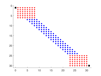
If the wave speeds are different in the two subdomains, for computational efficiency, different grid spacings are desirable so that the number of grid points per wavelength becomes the same in both subdomains [9, 12]. This leads to a mesh refinement interface with hanging nodes along $y=0$. Special care is therefore needed to couple the solutions along the interface. In the following, we consider a grid interface with mesh refinement ratio 1:2, and focus on the numerical treatment of the interface conditions (54). Other ratios can be treated analogously.

For simplicity, we consider periodic boundary conditions in $x$. For the spatial discretization, we use a Cartesian mesh with mesh size $h$ in the (fine) domain $\Omega^{f}$ and $2h$ in the (coarse) domain $\Omega^{c}$, see Figure 2.

Figure 2: A sketch of the grids $\boldsymbol{x}^{f}$ and $\boldsymbol{x}^{c}$.

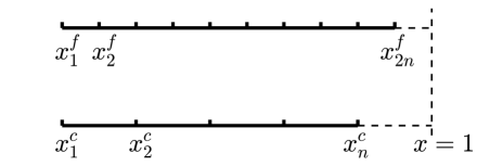
The number of grid points in the $x$ direction is $n$ in $\Omega^{c}$, and $2n$ in $\Omega^{f}$, where $h=1/(2n)$. We have excluded grid points on the periodic boundary $x=1$, because the solution at $x=1$ is the same as at $x=0$. The grid points $(\boldsymbol{x}^{f},\boldsymbol{y}^{f})$ in $\Omega^{f}$ and $(\boldsymbol{x}^{c},\boldsymbol{y}^{c})$ in $\Omega^{c}$ are defined as

$$\begin{cases}x^{f}_{i}=(i-1)h,\quad i=1,2,\cdots,2n,\\ y^{f}_{j}=(j-1)h,\quad j=0,1,2,\cdots,2n+1\end{cases}\text{and}\quad\begin{cases}x^{c}_{i}=2(i-1)h,\quad i=1,2,\cdots,n,\\ y^{c}_{j}=2(j-n)h,\quad j=0,1,2,\cdots,n+1\end{cases},$$ (55)

respectively. There are $2n$ ghost points

$$(x^{f}_{i},y^{f}_{0}),\ i=1,2,\cdots,2n$$ (56)

in $\Omega^{f}$ and $n$ ghost points

$$(x^{c}_{i},y^{c}_{n+1}),\ i=1,2,\cdots,n$$ (57)

in $\Omega^{c}$.

Notations for the two-dimensional SBP operators are introduced in Section 4.1. The SBP-GP method for the problem (53)-(54) is introduced in Section 4.2. A second order accurate method was originally developed in [22], where ghost points from both subdomains are used to impose the interface conditions. Here, we generalize the technique to fourth order accuracy. In Section 4.3, we propose a new SBP-GP method that only uses ghost points from the coarse domain. This reduces the amount of computational work for calculating the numerical solution at the ghost points and improves the structure of the associated linear system. We end this section with a discussion of the SBP-SAT method and its relation to the SBP-GP method.

4.1 SBP identities in two space dimensions

The one-dimensional SBP identities with ghost points (6) are on exactly the same form as those without ghost points, (7). In the discussion of SBP identities in two space dimensions, we use the notations for SBP operators with ghost points in $\Omega^{f}$. The same notational convention of the tilde symbol is used to indicate that the corresponding variable uses ghost points.

Let $\boldsymbol{u}$ and $\boldsymbol{v}$ be grid functions in $\Omega^{f}$. We define the two-dimensional scalar product

$$(\boldsymbol{u},\boldsymbol{v})_{h}=h^{2}\sum_{i=1}^{2n}\sum_{j=1}^{2n-1}w_{j}u_{ij}v_{ij}.$$

The weights $w_{j}$ do not depend on the index $i$ because of the periodic boundary condition in $x$. In addition, we define the scalar product for grid functions on the interface

$$\langle\boldsymbol{u}_{\Gamma},\boldsymbol{v}_{\Gamma}\rangle_{h}=h\sum_{i=1}^{2n}u_{i}v_{i},$$ (58)

where the subscript $\Gamma$ denotes the grid function on the interface.

The SBP identity in two space dimensions in the fine domain $\Omega^{f}$ can be written as

$$(\boldsymbol{u},G_{x}(\mu)\boldsymbol{v})_{h} =-S_{x}(\boldsymbol{u},\boldsymbol{v}),$$ (59)

$$(\boldsymbol{u},\widetilde{G}_{y}(\mu)\widetilde{\boldsymbol{v}})_{h} =-S_{y}(\boldsymbol{u},\boldsymbol{v})-\langle\boldsymbol{u}_{\Gamma},\widetilde{\boldsymbol{v}}^{\prime}_{\Gamma}\rangle_{h},$$ (60)

where the subscripts $x$ and $y$ denote the spatial direction that the operator acts on. The bilinear forms $S_{x}(\cdot,\cdot)$ and $S_{y}(\cdot,\cdot)$ are symmetric and positive semi-definite. There is no boundary term in (59) for $G_{x}(\mu)$ because of the periodic boundary condition. For simplicity, we have omitted the boundary term from the boundary at $y=1$. The last term on the right hand side of (60) corresponds to the boundary term from the interface, where the $i^{th}$ element of $\widetilde{\boldsymbol{v}}^{\prime}_{\Gamma}$ is

$$(v^{\prime}_{\Gamma})_{i}=\mu_{i,1}^{f}\widetilde{\boldsymbol{b}}_{1}^{T}\widetilde{\boldsymbol{v}}_{i,:}.$$ (61)

Here we use Matlab’s colon notation, i.e., $:$ denotes all grid points in the corresponding index direction.

To condense notation, we define

$$\widetilde{G}_{f}(\mu)=G_{x}(\mu)+\widetilde{G}_{y}(\mu),\quad S_{f}=S_{x}+S_{y},$$

so that (59)-(60) can be written as

$$(\boldsymbol{u},\widetilde{G}_{f}(\mu)\widetilde{\boldsymbol{v}})_{h}=-S_{f}(\boldsymbol{u},\boldsymbol{v})-\langle\boldsymbol{u}_{\Gamma},\widetilde{\boldsymbol{v}}^{\prime}_{\Gamma}\rangle_{h}.$$ (62)

The SBP identity for the operators in the coarse domain $\Omega^{c}$ are defined similarly.

4.2 The fourth order accurate SBP-GP method

We approximate (53) by

$$\boldsymbol{\rho^{f}}\boldsymbol{f}_{tt} =\widetilde{G}_{f}(\mu)\widetilde{\boldsymbol{f}},$$ (63)

$$\boldsymbol{\rho^{c}}\boldsymbol{c}_{tt} =\widetilde{G}_{c}(\mu)\widetilde{\boldsymbol{c}},$$ (64)

where the grid functions $\boldsymbol{f}$ and $\boldsymbol{c}$ are finite difference approximations of the functions $F(x,y,t)$ and $C(x,y,t)$ in (53), respectively. The diagonal matrices $\boldsymbol{\rho}^{f}$ and $\boldsymbol{\rho}^{c}$ contain the material properties $\rho^{f}$ and $\rho^{c}$ evaluated on the fine and coarse grids, respectively. Corresponding to the continuous interface condition (54), the grid functions $\boldsymbol{f}$ and $\boldsymbol{c}$ are coupled through the discrete interface conditions

$$\boldsymbol{f}_{\Gamma} =\mathcal{P}\boldsymbol{c}_{\Gamma},$$ (65)

$$\widetilde{\boldsymbol{c}}^{\prime}_{\Gamma} =\mathcal{R}\widetilde{\boldsymbol{f}}^{\prime}_{\Gamma}.$$ (66)

Here, $\mathcal{P}$ is an operator that interpolates a coarse interface grid function to an interface grid function on the fine grid. The operator $\mathcal{R}$ performs the opposite operation. It restricts an interface grid function on the fine grid to the coarse grid. Stability of the difference approximation relies on the compatibility between the operators $\mathcal{P}$ and $\mathcal{R}$, as is specified in the following theorem.

Theorem 1.

The semi-discretization (63)-(66) satisfies the energy estimate

$$\frac{d}{dt}\left[(\boldsymbol{f}_{t},\boldsymbol{\rho^{f}}\boldsymbol{f}_{t})_{h}+S_{f}(\boldsymbol{f},\boldsymbol{f})+(\boldsymbol{c}_{t},\boldsymbol{\rho^{c}}\boldsymbol{c}_{t})_{2h}+S_{c}(\boldsymbol{c},\boldsymbol{c})\right]=0,$$ (67)

if the interpolation and restriction operators are compatible,

$$\mathcal{P}=2\mathcal{R}^{T}.$$ (68)

Proof.

By using the SBP identity (62) in $\Omega^{f}$, we obtain

$$(\boldsymbol{f}_{t},\boldsymbol{\rho^{f}}\boldsymbol{f}_{tt})_{h}+S_{f}(\boldsymbol{f}_{t},\boldsymbol{f})=-\left\langle\left(\boldsymbol{f}_{\Gamma}\right)_{t},\widetilde{\boldsymbol{f}}^{\prime}_{\Gamma}\right\rangle_{h}.$$

Similarly, we have in $\Omega^{c}$

$$(\boldsymbol{c}_{t},\boldsymbol{\rho^{c}}\boldsymbol{c}_{tt})_{2h}+S_{c}(\boldsymbol{c}_{t},\boldsymbol{c})=\left\langle\left(\boldsymbol{c}_{\Gamma}\right)_{t},\widetilde{\boldsymbol{c}}^{\prime}_{\Gamma}\right\rangle_{2h}.$$

Summing the above two equations yields

$$\frac{d}{dt}\left[(\boldsymbol{f}_{t},\boldsymbol{\rho^{f}}\boldsymbol{f}_{t})_{h}+S_{f}(\boldsymbol{f},\boldsymbol{f})+(\boldsymbol{c}_{t},\boldsymbol{\rho^{c}}\boldsymbol{c}_{t})_{2h}+S_{c}(\boldsymbol{c},\boldsymbol{c})\right]=-2\left\langle\left(\boldsymbol{f}_{\Gamma}\right)_{t},\widetilde{\boldsymbol{f}}^{\prime}_{\Gamma}\right\rangle_{h}+2\left\langle\left(\boldsymbol{c}_{\Gamma}\right)_{t},\widetilde{\boldsymbol{c}}^{\prime}_{\Gamma}\right\rangle_{2h}.$$ (69)

To prove that the right-hand side vanishes, we first differentiate (65) in time, and use (58) to obtain

$$\left\langle\left(\boldsymbol{f}_{\Gamma}\right)_{t},\widetilde{\boldsymbol{f}}^{\prime}_{\Gamma}\right\rangle_{h}=\left\langle\left(\mathcal{P}\boldsymbol{c}_{\Gamma}\right)_{t},\widetilde{\boldsymbol{f}}^{\prime}_{\Gamma}\right\rangle_{h}.$$

The compatibility condition (68), together with the scalar product (58), gives

$$\left\langle\left(\mathcal{P}\boldsymbol{c}_{\Gamma}\right)_{t},\widetilde{\boldsymbol{f}}^{\prime}_{\Gamma}\right\rangle_{h}=\left\langle\left(\boldsymbol{c}_{\Gamma}\right)_{t},\mathcal{R}\widetilde{\boldsymbol{f}}^{\prime}_{\Gamma}\right\rangle_{2h}.$$

The second interface condition (66) leads to

$$\left\langle\left(\boldsymbol{c}_{\Gamma}\right)_{t},\mathcal{R}\widetilde{\boldsymbol{f}}^{\prime}_{\Gamma}\right\rangle_{2h}=\left\langle\left(\boldsymbol{c}_{\Gamma}\right)_{t},\widetilde{\boldsymbol{c}}^{\prime}_{\Gamma}\right\rangle_{2h}.$$ (70)

The energy rate relation (67) follows by inserting (70) into the right hand side of (69). This proves the theorem. ∎

We note that the factor 2 in the compatibility condition (68) arises because of the 1:2 mesh refinement ratio in two dimension and the periodic boundary condition. The factor is 4 in the corresponding three dimensional case.

For the mesh refinement ratio 1:2, the stencils in $\mathcal{P}$ and $\mathcal{R}$ can be easily computed by a Taylor series expansion. For example, a fourth order interpolation operator in (65) has the stencil

$$(f_{\Gamma})_{2i} =-\frac{1}{16}(c_{\Gamma})_{i-1}+\frac{9}{16}(c_{\Gamma})_{i}+\frac{9}{16}(c_{\Gamma})_{i+1}-\frac{1}{16}(c_{\Gamma})_{i+2},$$

$$(f_{\Gamma})_{2i-1} =(c_{\Gamma})_{i}$$

on the hanging and coinciding nodes, respectively. Then, the compatibility condition (68) determines the restriction operator $\mathcal{R}$, used by the second interface condition (66),

$$(c^{\prime}_{\Gamma})_{i}=-\frac{1}{32}(f^{\prime}_{\Gamma})_{2i-4}+\frac{9}{32}(f^{\prime}_{\Gamma})_{2i-2}+\frac{1}{2}(f^{\prime}_{\Gamma})_{2i-1}+\frac{9}{32}(f^{\prime}_{\Gamma})_{2i}-\frac{1}{32}(f^{\prime}_{\Gamma})_{2i+2}.$$

For other mesh refinement ratios, the interpolation and restriction operators can be constructed using the techniques in [11].

Similar to Dirichlet boundary conditions for the one-dimensional problem, ghost points are not explicitly involved in the first interface condition (65). However, by differentiating (65) twice in time and using the semi-discretized equations (63)-(64), we obtain

$$\left.\left(\boldsymbol{\rho^{f}}\right)^{-1}\widetilde{G}_{f}(\mu)\widetilde{\boldsymbol{f}}\right|_{\Gamma}=\mathcal{P}\left(\left.\left(\boldsymbol{\rho^{c}}\right)^{-1}\widetilde{G}_{c}(\mu)\widetilde{\boldsymbol{c}}\right|_{\Gamma}\right).$$ (71)

This condition depends on the ghost point values on both sides of the interface and is equivalent to (65) if the initial data also satisfies that condition. For this reason, we impose interface conditions for the semi-discrete problem through (66) and (71). When discretizing (63)-(64) in time by the predictor-corrector method, the fully discrete time-stepping method follows by the same principle as the predictor-corrector method in Algorithm 2. More precisely, for the predictor, step 2a is used to enforce (66) and step 2b is used for (65). Similarily, for the corrector, step 5a is used to enforce (66), combined with step 5b for (65).

The grid function $\widetilde{\boldsymbol{c}}^{\prime}_{\Gamma}$ in (66) has $n$ elements. By writing (66) in element-wise form it becomes clear that it is a system of $n$ linear equations that depends on $3n$ unknown ghost point values. Similarly, (71) is a system of $2n$ linear equations for the same $3n$ unknowns. In combination, the two interface conditions give a system of $3n$ linear equations, whose solution determines the $3n$ ghost point values. For the fully discrete problem, this linear system must be solved once during the predictor step and once during the corrector step.

The coefficients in the linear equations are independent of time. As a consequence, an efficient solution strategy is to LU-factorize the interface system once, before the time stepping starts. Backward substitution can then be used to calculate the ghost point values during the time-stepping. For problems in three space dimensions, computations are performed on many processors on a parallel distributed memory machine. Then it may not be straightforward to efficently calculate the LU-factorization. As an alternative, iterative solvers can be used. For example, an iterative block Jacobi relaxation method is used in [22]. It has proven to work well in practice for large-scale problems.

4.3 The improved SBP-GP method

Figure 3: A mesh refinement interface with ghost points denoted by filled circles. (a) ghost points from both domains. (b) ghost points from the coarse domain.

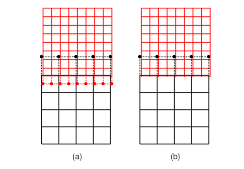
In the improved SBP-GP method, the interface conditions are imposed through $n$ linear equations that only depend on the $n$ ghost point values in $\widetilde{\boldsymbol{c}}$, see Figure 3 (b). The key to the improved method is to combine SBP operators with and without ghost points. More precisely, in $\Omega^{c}$ we use the SBP operator with ghost points. Thus, the semi-discretized equation in $\Omega^{c}$ is the same as in the original SBP-GP method,

$$\boldsymbol{\rho^{c}}\boldsymbol{c}_{tt}=\widetilde{G}_{c}(\mu)\boldsymbol{\widetilde{c}}.$$ (72)

In $\Omega^{f}$, we use (63) only for the grid points that are not on the interface

$$(\boldsymbol{\rho^{f}}\boldsymbol{f}_{tt})_{:,j}=(G_{f}(\mu)\boldsymbol{f})_{:,j},\quad j=2,3,\ldots.$$ (73)

For the grid points in $\Omega^{f}$ that are on the interface, we enforce the interface condition (65) such that

$$\boldsymbol{f}_{:,1}=\mathcal{P}(\boldsymbol{c}_{:,n}).$$ (74)

Note that this equation does not depend on any ghost point values in $\Omega^{f}$.

To write the semi-discretization in a compact form and prepare for the energy analysis, we differentiate (74) twice in time, and use (72) to obtain

$$\left(\boldsymbol{f}_{tt}\right)_{:,1}=\mathcal{P}\left((\boldsymbol{c}_{tt})_{:,n}\right)=\mathcal{P}\left(\left.\left(\boldsymbol{\rho}^{c}\right)^{-1}\widetilde{G}_{c}(\mu)\widetilde{\boldsymbol{c}}\right|_{\Gamma}\right).$$ (75)

Equations (73) and (75) can be combined into

$$\left(\boldsymbol{\rho^{f}}\boldsymbol{f}_{tt}\right)_{:,j}:=\left(L_{h}\boldsymbol{f}\right)_{:,j}=\begin{cases}\left(G_{f}(\mu)\boldsymbol{f}\right)_{:,1}+\boldsymbol{\eta}_{:},&j=1,\\ \left(G_{f}(\mu)\boldsymbol{f}\right)_{:,j},&j=2,3,\ldots,\end{cases}$$ (76)

where

$$\boldsymbol{\eta}=\boldsymbol{\rho^{f}}|_{\Gamma}\mathcal{P}\left(\left.\left(\boldsymbol{\rho^{c}}\right)^{-1}\widetilde{G}_{c}(\mu)\boldsymbol{\widetilde{c}}\right|_{\Gamma}\right)-\left.G_{f}(\mu)\boldsymbol{f}\right|_{\Gamma}.$$

We note that $\boldsymbol{\eta}$ is a zero vector up to truncation errors in the SBP operator and the interpolation operator. Therefore, $\boldsymbol{\eta}$ does not affect the order of accuracy in the spatial discretization.

The semi-discretization (72) and (76) can be viewed as a hybridization of the SBP-GP method and the SBP-SAT method. The spatial discretization (76) in $\Omega^{f}$ is on the SBP-SAT form, but the penalty term $\boldsymbol{\eta}$ depends on the ghost points values in $\widetilde{\boldsymbol{c}}$.

Continuity of the solution is imposed by (74), in the same way as in the original SBP-GP method. But to account for the contribution from $\boldsymbol{\eta}$, continuity of flux (the second interface condition in (54)) must be imposed differently. Here we use

$$\widetilde{\boldsymbol{c}}^{\prime}_{\Gamma}=\mathcal{R}\left(\boldsymbol{f}^{\prime}_{\Gamma}-hw_{1}\boldsymbol{\eta}\right),$$ (77)

where $h$ is the mesh size in $\Omega_{f}$, and $w_{1}$ is the first entry in the scalar product (3). Note that ghost points are used to compute $\widetilde{\boldsymbol{c}}^{\prime}_{\Gamma}$ but not $\boldsymbol{f}^{\prime}_{\Gamma}$.

Compared with (66) in the original SBP-GP method, the condition (77) includes the term $hw_{1}\boldsymbol{\eta}$. Because it is on the order of the truncation error it does not affect the order of accuracy. As a consequence, (77) provides a valid way of enforcing flux continuity. The following theorem illustrates why the $\boldsymbol{\eta}$-term is important for energy stability.

Theorem 2.

Assume that the interpolation and restriction operators satify (68). Then, the semi-discrete approximation (72), (76) and (77) is energy stable in the sense that (67) holds.

Proof.

From (76) , we have

$$\left(\boldsymbol{f}_{t},\boldsymbol{\rho^{f}}\boldsymbol{f}_{tt}\right)_{h} =\left(\boldsymbol{f}_{t},G_{f}(\mu)\boldsymbol{f}\right)_{h}+hw_{1}\left\langle\boldsymbol{f}_{t}|_{\Gamma},\boldsymbol{\eta}\right\rangle_{h}$$

$$=-S_{f}(\boldsymbol{f}_{t},\boldsymbol{f})-\left\langle\boldsymbol{f}_{t}|_{\Gamma},\boldsymbol{f}^{\prime}_{\Gamma}\right\rangle_{h}+hw_{1}\left\langle\boldsymbol{f}_{t}|_{\Gamma},\boldsymbol{\eta}\right\rangle_{h}$$

$$=-S_{f}(\boldsymbol{f}_{t},\boldsymbol{f})+\left\langle\boldsymbol{f}_{t}|_{\Gamma},-\boldsymbol{f}^{\prime}_{\Gamma}+hw_{1}\boldsymbol{\eta}\right\rangle_{h}.$$

The contribution from the domain $\Omega^{c}$ is

$$(\boldsymbol{c}_{t},\boldsymbol{\rho^{c}}\boldsymbol{c}_{tt})_{2h}=-S_{c}(\boldsymbol{c}_{t},\boldsymbol{c})+\langle\boldsymbol{c}_{t}|_{\Gamma},\widetilde{\boldsymbol{c}}^{\prime}_{\Gamma}\rangle_{2h}.$$

Adding the two above equations gives

$$\frac{d}{dt}\left[(\boldsymbol{f}_{t},\boldsymbol{\rho^{f}}\boldsymbol{f}_{t})_{h}+S_{f}(\boldsymbol{f},\boldsymbol{f})+(\boldsymbol{c}_{t},\boldsymbol{\rho^{c}}\boldsymbol{c}_{t})_{2h}+S_{c}(\boldsymbol{c},\boldsymbol{c})\right]=2\langle\boldsymbol{f}_{t}|_{\Gamma},-\boldsymbol{f}^{\prime}_{\Gamma}+hw_{1}\boldsymbol{\eta}\rangle_{h}+2\left\langle\boldsymbol{c}_{t}|_{\Gamma},\widetilde{\boldsymbol{c}}^{\prime}_{\Gamma}\right\rangle_{2h}\\ =2\langle\mathcal{P}\boldsymbol{c}_{t}|_{\Gamma},-\boldsymbol{f}^{\prime}_{\Gamma}+hw_{1}\boldsymbol{\eta}\rangle_{h}+2\langle\boldsymbol{c}_{t}|_{\Gamma},\widetilde{\boldsymbol{c}}^{\prime}_{\Gamma}\rangle_{2h}=2\langle\boldsymbol{c}_{t}|_{\Gamma},\mathcal{R}(-\boldsymbol{f}^{\prime}_{\Gamma}+hw_{1}\boldsymbol{\eta})\rangle_{2h}+2\langle\boldsymbol{c}_{t}|_{\Gamma},\widetilde{\boldsymbol{c}}^{\prime}_{\Gamma}\rangle_{2h}=0.$$

∎

With the predictor-corrector method for the time discretization of (72) and (76), the fully discrete algorithm can be adopted from Algorithm 2. We impose (77) in step 2a for the predictor, and in step 5a for the corrector. We note that (77) corresponds to a system of $n$ linear equations. The right-hand sides are different in the linear systems in steps 2a and 5a, but the matrix is the same. It can therefore be LU-factorized once, before time integration starts. The linear systems can then be solved by backward substitution during the time stepping. The improved SBP-GP method presented in this section is evaluated through numerical experiments in Section 5.

4.4 The SBP-SAT method

In the SBP-SAT method, the penalty terms for the interface conditions (54) can be constructed by combining the penalty terms for the Neumann problem in Section 3.1 and the Dirichlet problem in Section 3.2. The semi-discretization can be written as

$$\boldsymbol{\rho^{f}}\boldsymbol{f}_{tt} =G_{f}(\mu)\boldsymbol{f}+\boldsymbol{p_{f}},$$ (78)

$$\boldsymbol{\rho^{c}}\boldsymbol{c}_{tt} =G_{c}(\mu)\boldsymbol{c}+\boldsymbol{p_{c}}.$$ (79)

There are two choices of $\boldsymbol{p_{f}}$ and $\boldsymbol{p_{c}}$. The first version, developed in [31], uses three penalty terms

$$(p_{f})_{i,:}=W^{-1}_{f}\left[-\mu_{i,1}^{f}\frac{1}{2}\boldsymbol{b}_{1}^{f}\left(\boldsymbol{f}_{\Gamma}-\mathcal{P}\boldsymbol{c}_{\Gamma}\right)_{i}-\mu_{i,1}^{f}\frac{\tau_{f}}{h}\boldsymbol{e}_{1}^{f}\left(\boldsymbol{f}_{\Gamma}-\mathcal{P}\boldsymbol{c}_{\Gamma}\right)_{i}+\frac{1}{2}\boldsymbol{e}_{1}^{f}\left(\boldsymbol{f}^{\prime}_{\Gamma}-\mathcal{P}\boldsymbol{c}^{\prime}_{\Gamma}\right)_{i}\right],$$ (80)

$$(p_{c})_{i,:}=W^{-1}_{c}\left[-\mu_{i,1}^{c}\frac{1}{2}\boldsymbol{b}_{1}^{c}\left(\boldsymbol{c}_{\Gamma}-\mathcal{R}\boldsymbol{f}_{\Gamma}\right)_{i}-\mu_{i,1}^{c}\frac{\tau_{c}}{2h}\boldsymbol{e}_{1}^{c}\left(\boldsymbol{c}_{\Gamma}-\mathcal{R}\boldsymbol{f}_{\Gamma}\right)_{i}+\frac{1}{2}\boldsymbol{e}_{1}^{c}\left(\boldsymbol{c}^{\prime}_{\Gamma}-\mathcal{R}\boldsymbol{f}^{\prime}_{\Gamma}\right)_{i}\right],$$ (81)

where $\boldsymbol{b}_{1}$ and $\boldsymbol{e}_{1}$ act in the $y$ direction. In both (80) and (81), the first two terms penalize continuity of the solution, and the third term penalizes continuity of the flux. The scheme (78)-(81) is energy stable when the penalty parameters satisfy

$$\tau_{f}=\frac{1}{2}\tau_{c}\geq\max_{i,j}\left(\frac{(\mu^{f}_{i,1})^{2}}{2(\mu_{\min}^{f})_{i}\alpha},\frac{(\mu^{c}_{j,n})^{2}}{2(\mu_{\min}^{c})_{j}\alpha}\right),$$ (82)

where $i=1,2,\ldots,2n$ and $j=1,2,\ldots,n$.

The second choice of SATs uses four penalty terms [28], which has a better stability property for problems with curved interfaces. The method was improved further in [1] from the accuracy perspective when non-periodic boundary conditions are used in the $x$-direction. In addition, the penalty parameters in [1] are optimized and are sharper than those in [28]. As will be seen in the numerical experiments, the sharper penalty parameters lead to an improved CFL condition.

4.5 Computational complexity

In the next section, we test numerically the CFL condition of the improved SBP-GP method and the SBP-SAT method for cases with a grid refinement interface. To enable a fair comparison in terms of computational efficiency, in this section we estimate the computational cost of the two methods for one time step. Since the interior stencils of the two SBP operators are the same, the main difference in computational cost comes from how the interface conditions are imposed at each time step. For simplicity, we only consider problems with constant coefficients when estimating the computational complexity. Also note that the number of floating point operations (flops) stated below depends on the implementation of the algorithms, and should not be considered exact.

In the improved SBP-GP method, a system of $n$ linear equations must be solved at each time step, where $n$ is the number of grid points on the interface in the coarse domain. The system matrix is banded with bandwidth 7, so the LU factorization requires $49n$ flops, but it is only computed once before the time stepping begins. In each time step, updating the right hand side of the linear system and solving by backward substitution requires $173n$ and $5n$ flops, respectively. This results in a grand total of $178n$ flops at each time step.

In the SBP-SAT method, the interface conditions are imposed by the SAT terms, which are updated at each time step. This calculation requires $157n$ flops. We conclude that imposing interface conditions with the SBP-GP and the SBP-SAT method require a comparable number of floating point operations per time step. Thus, the main difference in computational efficiency comes from the different CFL stability restrictions on the time step, which is investigated in the following section.

5 Numerical experiments

In this section, we conduct numerical experiments to compare the SBP-GP method and the SBP-SAT method in terms of computational efficiency. Our first focus is CFL condition, which is an important factor in solving large-scale problems. We numerically test the effect of different boundary and interface techniques on the CFL condition with the predictor-corrector time stepping method. We then compare $L^{2}$ error and convergence rate of the SBP-GP method and the SBP-SAT method with the same spatial and temporal discretizations. The convergence rate is computed by

$$\log\left(\frac{e_{h}}{e_{2h}}\right)\bigg{/}\log\left(\frac{1}{2}\right),$$

where $e_{2h}$ is the $L^{2}$ error on a grid $\boldsymbol{x}$, and $e_{h}$ is the $L^{2}$ error on a grid with grid size half of $\boldsymbol{x}$ in each subdomain and spatial direction.

5.1 Time-stepping stability restrictions

We consider the scalar wave equation in one space dimension

$$\rho U_{tt}=(\mu U_{x})_{x}+F,$$ (83)

in the domain $x\in[-\pi/2,\pi/2]$ with non-periodic boundary conditions.

In [26], it is proved that for the predictor-corrector time stepping method, the time step constraint by the CFL condition is

$$\delta_{t}\leq\frac{2\sqrt{3}}{\sqrt{\kappa}},$$ (84)

where $\kappa$ is the spectral radius of the spatial discretization matrix. In general, we do not have a closed form expression for $\kappa$. In the special case of periodic boundary conditions and constant coefficients, $\kappa$ is given by the following lemma.

Lemma 1.

Consider (83) with periodic boundary conditions, constant $\rho$, $\mu$ and zero forcing $F=0$. If the equation is discretized with standard fourth order accurate centered finite differences, the spectral radius becomes

$$\kappa=\frac{16\mu}{3h^{2}\rho},$$

where $h$ is the grid spacing.

Proof.

See Appendix 1. ∎

In the following numerical experiments, we choose $\rho=\mu=1$, which gives the estimated CFL condition $\delta_{t}\leq 1.5h$. This case is used below as a reference when comparing CFL conditions.

First, we consider the Neumann boundary condition at $x=\pm\pi/2$, and use the SBP-GP and the SBP-SAT method to solve the equation (83) until $t=200$. For the SBP-GP method with the fourth order SBP operator derived in [26], we find that the scheme is stable when $\delta_{t}\leq 1.44h$. In other words, the time step needs to be reduced by about $4\%$ when comparing with the reference CFL condition. For the SBP-SAT method with the fourth order SBP operator derived in [19], the scheme is stable up to the reference CFL condition $\delta_{t}\leq 1.5h$.

Next, we consider the equation with Dirichlet boundary conditions at $x=\pm\pi/2$. To test the injection method and the SAT method, we use the fourth order accurate SBP operator without ghost point [19]. When using the injection method to impose the Dirichlet boundary condition, the scheme is stable with $\delta_{t}\leq 1.5h$. However, when using the SAT method to weakly impose the Dirichlet boundary condition and choosing the penalty parameter $20\%$ larger than its stability-limiting value, the scheme is only stable if $\delta_{t}\leq 1.16h$. This amounts to a reduction in time step by $23\%$. If we decrease the penalty parameter so that it is only $0.1\%$ larger than its stability-limiting value, then the scheme is stable with $\delta_{t}\leq 1.25h$, i.e. the time step needs to be reduced by $17\%$, compared to the injection method.

In conclusion, for the Neumann boundary condition, both the SBP-GP and the SBP-SAT method can be used with a time step comparable to that given by the reference CFL condition. This is not surprising, given the similarity of the methods and in the discrete energy expressions. For the Dirichlet boundary condition, we need to reduce the time step by $23\%$ in the SAT method. If we instead inject the Dirichlet data, then the scheme is stable with the time step given by the reference CFL condition.

5.2 Discontinuous material properties

We now investigate the SBP-GP and SBP-SAT method for the wave equation with a mesh refinement interface. The model problem is

$$\rho U_{tt}=\nabla\cdot(\mu\nabla U)+F,$$ (85)

in a two-dimensional domain $\Omega=[0,4\pi]\times[-4\pi,4\pi]$, where $\rho(x,y)>0$, $\mu(x,y)>0$, and the wave speed is $c=\sqrt{\mu/\rho}$. Equation (85) is augmented with Dirichlet boundary conditions at $y=\pm 4\pi$, and periodic boundary conditions at $x=0$ and $x=4\pi$.

The domain $\Omega$ is divided into two subdomains $\Omega^{1}=[0,4\pi]\times[-4\pi,0]$ and $\Omega^{2}=[0,4\pi]\times[0,4\pi]$ with an interface $\Gamma$ at $y=0$. The material parameter $\mu$ is a smooth function in each subdomain, but may be discontinuous across the interface. In particular, we consider two cases: $\mu$ is piecewise constant in Section 5.2, and $\mu$ is a smooth function in Section 5.3. In each case, we test the fourth order accurate SBP-GP method and the SBP-SAT method, both in terms of the CFL condition and the convergence rate.

When $\mu$ is piecewise constant, an analytical solution can be constructed by Snell’s law. We choose a unit density $\rho=1$ and denote the piecewise constant $\mu$ as

$$\mu(x,y)=\begin{cases}\mu_{1},\quad&(x,y)\in\Omega^{1},\\ \mu_{2},\quad&(x,y)\in\Omega^{2},\end{cases}$$

where $\mu_{1}\neq\mu_{2}$.

Figure 4: The exact solution at time $t=0$ (left), and $t=11$ (right) when the wave has propagated for about 2.5 temporal periods. The solution is continuous at the material interface $x=0$ but the normal derivative is discontinuous due to the material discontinuity.

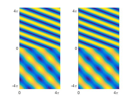
Let an incoming plane wave $U_{I}$ travel in $\Omega^{1}$ and impinge on the interface $\Gamma$. The resulting field consists of the incoming wave $U_{I}$, as well as a reflected field $U_{R}$ and a transmitted field $U_{T}$. With the ansatz

$$\begin{split}&U_{I}=\cos(x+y-\sqrt{2\mu_{1}}t),\\ &U_{R}=R\cos(-x+y+\sqrt{2\mu_{1}}t),\\ &U_{T}=T\cos(x+ky-\sqrt{2\mu_{1}}t),\end{split}$$

where $k=\sqrt{2\mu_{1}/\mu_{2}-1}$, the two parameters $R$ and $T$ are determined by the interface conditions

$$\begin{split}U_{I}+U_{R}&=U_{T},\\ {\mu_{1}}\frac{\partial}{\partial x}(U_{I}+U_{R})&={\mu_{2}}\frac{\partial}{\partial x}U_{T},\end{split}$$

yielding $R=(\mu_{1}-\mu_{2}k)/(\mu_{1}+\mu_{2}k)$ and $T=1+R$.

In the following experiments, we choose $\mu_{1}=1$ and $\mu_{2}=0.25$. As a consequence, the wave speed is $c_{1}=1$ in $\Omega^{1}$ and $c_{2}=0.5$ in $\Omega^{2}$. To keep the number of grid points per wavelength the same in two subdomains, we use a coarse grid with grid spacing $2h$ in $\Omega^{1}$, and a fine grid with grid spacing $h$ in $\Omega^{2}$. We let the wave propagate from $t=0$ until $t=11$. The exact solution at these two points in time are shown in Figure 4.

5.2.1 CFL condition

To derive an estimated CFL condition, we perform a Fourier analysis in each subdomain $\Omega^{1}$ and $\Omega^{2}$. Assuming periodicity in both spatial directions, the spectral radius of the spatial discretization in $\Omega^{1}$ and $\Omega^{2}$ is the same $\kappa=4/(3h^{2})$, given by Lemma 1. By using (84), we find that the estimated CFL condition is

$$\delta_{t}\leq\frac{1}{\sqrt{2}}\frac{2\sqrt{3}}{\sqrt{4/(3h^{2})}}=\frac{3}{\sqrt{2}}h\approx 2.12h.$$ (86)

We note that the restriction on time step is the same in both subdomains. The factor $1/\sqrt{2}$ in (86), which is not present in (84), comes from (85) having two space dimensions.

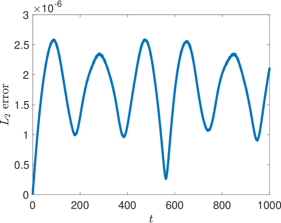
For the SBP-GP method, we have found numerically that the method is stable when the time step $\delta_{t}\leq 2.09h$. This indicates that the non-periodic boundary condition and the non-conforming grid interface do not affect time step restriction of the SBP-GP method. With $\delta_{t}=2.09h$ and $641^{2}$ grid points in the coarse domain, we perform a long time simulation until $t=1000$, and plot the $L_{2}$ error in Figure 5. We observe that the $L_{2}$ error does not grow in time, which verifies that the discretization is stable.

Figure 5: $L_{2}$ error for the improved SBP-GP method for a long time simulation to time $t=1000$ ($\sim$ 225 temporal periods).

For the SBP-SAT method with three penalty terms, the stability limit appears to be $\delta_{t}\leq 1.18h$, which represents approximately a 45% reduction in the time step. When using four penalty terms and the sharper penalty parameters [1], the scheme is stable for $\delta_{t}\leq 1.82h$, which is an improvement from the scheme with three penalty terms, but not as good as the SBP-GP method.

5.2.2 Conditioning and sparsity of the linear system for ghost points

In the SBP-GP method, a system of linear equations needs to be solved to compute the solution at the ghost points. To demonstrate the superiority of the improved SBP-GP method, we examine the conditioning and sparsity of the system on three meshes.

$N_{c}$	$cond_{i}$	$cond_{o}$	$nnz_{i}$	$nnz_{o}$
$321^{2}$	1.26	778	2240	4160
$641^{2}$	1.26	1680	4480	8320
$1281^{2}$	1.26	3425	8960	16640

Table 1: Condition number $cond$ and number of nonzero elements $nnz$ in the matrix for ghost points. The subscript $o$ and $i$ correspond to the original and improved SBP-GP method, respectively. $N_{c}$ denotes the number of grid points in the coarse domain.

In Table 1, we observe that for the improved SBP-GP method, the condition number is close to one and is independent of the mesh size. In contrast, the condition number in the original SBP-GP method is several magnitudes larger, and grows with mesh refinement. Furthermore, the number of nonzero elements in the improved SBP-GP matrix is approximately half the number of nonzero elements in the matrix in the original method. Hence, the system of linear equations in the improved SBP-GP method is both more sparse and better conditioned.

5.2.3 Convergence rate

We now perform a convergence study for the SBP-GP method and the SBP-SAT method. We choose the time step $\delta_{t}=h$ so that both methods are stable. The $L^{2}$ errors in the numerical solution with the SBP-GP method are shown in Table 2. Though the dominating truncation error is $\mathcal{O}(h^{2})$ at grid points near boundaries, the numerical solution converges to fourth order accuracy, i.e. two orders are gained in convergence rate [29].

$2h$	$L^{2}$ error (rate)
1.57$\times 10^{-1}$	1.6439$\times 10^{-3}$
7.85$\times 10^{-2}$	1.0076$\times 10^{-4}$ (4.02)
3.93$\times 10^{-2}$	6.2738$\times 10^{-6}$ (4.01)
1.96$\times 10^{-2}$	3.9193$\times 10^{-7}$ (4.00)
9.81$\times 10^{-3}$	2.4344$\times 10^{-8}$ (4.01)

Table 2: $L^{2}$ errors (convergence rates) of the fourth order SBP-GP method for piecewise constant $\mu$.

For the SBP-SAT method with three penalty terms (78)-(81), the $L^{2}$ errors labeled as SAT3 in Table 3 only converge at a rate of three. Because the dominating truncation error is $\mathcal{O}(h^{2})$ at grid points close to boundaries, we gain only one order of accuracy in the numerical solution. This suboptimal convergence behavior has also been observed in other settings [29].

$2h$	$L^{2}$ error (rate) SAT3	$L^{2}$ error (rate) SAT4	$L^{2}$ error (rate) INT6
1.57$\times 10^{-1}$	3.0832$\times 10^{-3}$	2.1104$\times 10^{-3}$	2.1022$\times 10^{-3}$
7.85$\times 10^{-2}$	3.4792$\times 10^{-4}$ (3.15)	1.1042$\times 10^{-4}$ (4.26)	1.1014$\times 10^{-4}$ (4.25)
3.93$\times 10^{-2}$	4.4189$\times 10^{-5}$ (2.98)	6.6902$\times 10^{-6}$ (4.04)	6.6815$\times 10^{-6}$ (4.04)
1.96$\times 10^{-2}$	5.6079$\times 10^{-6}$ (2.98)	4.0374$\times 10^{-7}$ (4.05)	4.0346$\times 10^{-7}$ (4.05)
9.81$\times 10^{-3}$	7.0745$\times 10^{-7}$ (2.99)	2.4659$\times 10^{-8}$ (4.03)	2.4651$\times 10^{-8}$ (4.03)

Table 3: $L^{2}$ errors (convergence rates) of the fourth order SBP-SAT method for piecewise constant $\mu$.

We have found two simple remedies to obtain a fourth order convergence rate. First, when using the SBP-SAT method with four penalty terms, we obtain a fourth order convergence rate, as shown in the third column of Table 3 labeled as SAT4. Alternatively, we can use three penalty terms but employ a sixth order interpolation and restriction operators at the non-conforming interface. This also leads to a fourth order convergence rate, see the fourth column of Table 3, labeled INT6. In both approaches, the dominating truncation error is still $\mathcal{O}(h^{2})$ at a few grid points close to the boundaries. However, different penalty terms will give different boundary systems in the normal mode analysis for convergence rate. The precise rate of convergence can be analyzed by the Laplace-transform method, but is beyond the scope of this paper.

We also observe that the $L^{2}$ errors of the SBP-GP method is almost identical to that of the SBP-SAT method (SAT4 and INT6) with the same mesh size.

5.3 Smooth material parameters

In this section, we test the two methods when the material parameters are smooth functions in the whole domain $\Omega$. More precisely, we use material parameters

$$\begin{split}\rho&=-\cos(x)\cos(y)+3,\\ \mu&=\cos(x)\cos(y)+2.\end{split}$$

The forcing function and initial conditions are chosen so that the manufactured solution becomes

$$u(x,y,t)=\sin(x+2)\cos(y+1)\sin(t+3).$$

We use the same grid as in Section 5.2 with grid size $2h$ in $\Omega^{1}$ and $h$ in $\Omega^{2}$. The parameters $\rho_{\min}=2$ and $\mu_{\max}=3$ take the extreme values at the same grid point. Therefore, a Fourier analysis of the corresponding periodic problem gives the time step restriction

$$\delta_{t}\leq\frac{1}{\sqrt{2}}\frac{2\sqrt{3}}{\sqrt{16/(3h^{2})}\sqrt{\mu_{\max}/\rho_{\min}}}=\frac{\sqrt{3}}{2}h\approx 0.86h.$$

Numerically, we have found that the SBP-GP method is stable when $\delta_{t}\leq 0.86h$. This shows again that the non–periodicity and interface coupling do not affect the CFL condition in the SBP-GP method. The SBP-SAT method is stable with $\delta_{t}\leq 0.77h$, which means that the time step needs to be reduced by approximately 10%.

To test convergence, we choose the time step $\delta_{t}=0.7h$ so that both the SBP-GP method and SBP-SAT method are stable. The $L^{2}$ errors at $t=11$ are shown in Table 4 for the SBP-GP method. We observe a fourth order convergence rate.

$2h$	$L^{2}$ error (rate)
1.57$\times 10^{-1}$	2.7076$\times 10^{-4}$
7.85$\times 10^{-2}$	1.6000$\times 10^{-5}$ (4.08)
3.93$\times 10^{-2}$	9.7412$\times 10^{-7}$ (4.04)
1.96$\times 10^{-2}$	6.0183$\times 10^{-8}$ (4.02)
9.81$\times 10^{-3}$	3.7426$\times 10^{-9}$ (4.01)

Table 4: $L^{2}$ errors (convergence rates) of the SBP-GP method for smooth $\mu$.

Similar to the case with piecewise constant material property, the standard SBP-SAT method only converges to third order accuracy, see the second column of Table 5 labeled as SAT3. We have tested the SBP-SAT method with four penalty terms, or with a sixth order interpolation and restriction operator. Both methods lead to a fourth order convergence rate, see the third and fourth column in Table 5. However, the $L^{2}$ error is more than three times as large as the $L^{2}$ error of the SBP-GP method with the same mesh size.

$2h$	$L^{2}$ error (rate) SAT3	$L^{2}$ error (rate) SAT4	$L^{2}$ error (rate) INT6
1.57$\times 10^{-1}$	3.8636$\times 10^{-3}$	1.8502$\times 10^{-3}$	1.8503$\times 10^{-3}$
7.85$\times 10^{-2}$	4.3496$\times 10^{-4}$ (3.15)	9.4729$\times 10^{-5}$ (4.29)	9.4736$\times 10^{-5}$ (4.29)
3.93$\times 10^{-2}$	5.3152$\times 10^{-5}$ (3.03)	3.7040$\times 10^{-6}$ (4.68)	3.7043$\times 10^{-6}$ (4.68)
1.96$\times 10^{-2}$	6.6271$\times 10^{-6}$ (3.00)	2.0778$\times 10^{-7}$ (4.16)	2.0779$\times 10^{-7}$ (4.16)
9.81$\times 10^{-3}$	8.2783$\times 10^{-7}$ (3.00)	1.3372$\times 10^{-8}$ (3.96)	1.3372$\times 10^{-8}$ (3.96)

Table 5: $L^{2}$ errors (convergence rates) of the fourth order SBP-SAT method for smooth $\mu$.

6 Conclusion

We have analyzed two different types of SBP finite difference operators for solving the wave equation with variable coefficients: operators with ghost points, $\widetilde{G}(\mu)$, and operators without ghost points, $G(\mu)$. The close relation between the two operators has been analyzed and we have presented a way of adding or removing the ghost point dependence in the operators. Traditionally, the two operators have been used within different approaches for imposing the boundary conditions. Based on their relation, we have in this paper devised a scheme that combines both operators for satisfying the interface conditions at a non-conforming grid refinement interface.

We first used the SBP operator with ghost points to derive a fourth order accurate SBP-GP method for the wave equation with a grid refinement interface. This method uses ghost points from both sides of the refinement interface to enforce the interface conditions. Accuracy and stability of the method are ensured by using a fourth order accurate interpolation stencil and a compatible restriction stencil. Secondly, we presented an improved method, where only ghost points from the coarse side are used to impose the interface conditions. This is achieved by combining the operator $G(\mu)$ in the fine grid and the operator $\widetilde{G}(\mu)$ in the coarse grid. Compared to the first SBP-GP method, the improved method leads to a smaller system of linear equations for the ghost points with better conditioning. In addition, we have made improvements to the traditional fourth order SBP-SAT method, which only exhibits a third order convergence rate for the wave equation with a grid refinement interface. Two remedies have been presented and both result in a fourth order convergence rate.

We have conducted numerical experiments to verify that the proposed methods converge with fourth order accuracy, for both smooth and discontinuous material properties. With a discontinuous material, the domain is partitioned into subdomains such that discontinuities are aligned with subdomain boundaries. We have also found numerically that the proposed SBP-GP method is stable under a CFL time-step condition that is very close to the von Neumann limit for the corresponding periodic problem. Being able to use a large time step is essential for solving practical large-scale wave propagation problems, because the computational complexity grows linearly with the number of time steps. We have found that the SBP-SAT method requires a smaller time step for stability, and that the time step depends on the penalty parameters of the interface coupling conditions. In the case of smooth material properties, the SBP-SAT method was also found to yield to a larger solution error compared to the SBP-GP method, for the same grid sizes and time step.

One disadvantage of the SBP-GP method is that a system of linear equations must be solved to obtain the numerical solutions at the ghost points. However, previous work has demonstrated that the system can be solved very efficiently by an iterative method [23, 25]. Furthermore, the proposed method only uses ghost points on one side of the interface and therefore leads to a linear system with fewer unknowns and a more regular structure than previously.

Sixth order accurate SBP operators can be used in the proposed method in a straightforward way. However, sixth order SBP discretization often leads to a convergence rate lower than six, and it is an open question if a six order discretization is more efficient than a fourth order discretization for realistic problems. In future work we plan to extend the proposed method to the elastic wave equation in three space dimensions with realistic topography based on [23], and implement it on a distributed memory machine to evaluate its efficiency.

Appendix 1: Proof of Lemma 1

By using the standard fourth order finite difference stencil, (83) can be approximated as

$$\frac{d^{2}u_{j}}{dt^{2}}=\left(-\frac{1}{12}u_{j+2}+\frac{4}{3}u_{j+1}-\frac{5}{2}u_{j}+\frac{4}{3}u_{j-1}-\frac{1}{12}u_{j-2}\right)\frac{\mu}{\rho}.$$

By using the ansatz $u_{j}=\hat{u}e^{i\omega x_{j}}$, where $\omega$ is the wave number and $x_{j}=jh$, we obtain

$$\frac{d^{2}\hat{u}}{dt^{2}} =\left(-\frac{1}{12}e^{i\omega 2h}+\frac{4}{3}e^{i\omega h}-\frac{5}{2}+\frac{4}{3}e^{-i\omega h}-\frac{1}{12}e^{-i\omega 2h}\right)\frac{\mu}{\rho}\hat{u}$$

$$=-\frac{4}{h^{2}}\sin^{2}\frac{\omega h}{2}\left(1+\frac{1}{3}\sin^{2}\frac{\omega h}{2}\right)\frac{\mu}{\rho}\hat{u}.$$

Therefore, the Fourier transform of the fourth order accurate central finite difference stencil is

$$\hat{Q}=-\frac{4}{h^{2}}\sin^{2}\frac{\omega h}{2}\left(1+\frac{1}{3}\sin^{2}\frac{\omega h}{2}\right)\frac{\mu}{\rho}.$$ (87)

Consequently, we have

$$\kappa=\max|\hat{Q}|=\frac{16\mu}{3h^{2}\rho}.$$

References

- [1] M. Almquist, S. Wang, and J. Werpers, Order-preserving interpolation for summation-by-parts operators at nonconforming grid interfaces, SIAM J. Sci. Comput., 41 (2019), pp. A1201–A1227.
- [2] D. Appelö and G. Kreiss, Application of a perfectly matched layer to the nonlinear wave equation, Wave Motion, 44 (2007), pp. 531–548.
- [3] M. H. Carpenter, D. Gottlieb, and S. Abarbanel, Time–stable boundary conditions for finite–difference schemes solving hyperbolic systems: methodology and application to high–order compact schemes, J. Comput. Phys., 111 (1994), pp. 220–236.
- [4] K. Duru, G. Kreiss, and K. Mattsson, Stable and high–order accurate boundary treatments for the elastic wave equation on second–order form, SIAM J. Sci. Comput., 36 (2014), pp. A2787–A2818.
- [5] K. Duru and K. Virta, Stable and high order accurate difference methods for the elastic wave equation in discontinuous media, J. Comput. Phys., 279 (2014), pp. 37–62.
- [6] J. C. Gilbert and P. Joly, Higher order time stepping for second order hyperbolic problems and optimal CFL conditions, Springer, 2008, pp. 67–93.
- [7] K. F. Graff, Wave Motion in Elastic Solids, Dover Publications, 1991.
- [8] B. Gustafsson, The convergence rate for difference approximations to mixed initial boundary value problems, Math. Comput., 29 (1975), pp. 396–406.
- [9] T. Hagstrom and G. Hagstrom, Grid stabilization of high–order one–sided differencing II: second–order wave equations, J. Comput. Phys., 231 (2012), pp. 7907–7931.
- [10] J. S. Hesthaven and T. Warburton, Nodal Discontinuous Galerkin Methods, Springer, 2008.
- [11] J. E. Kozdon and L. C. Wilcox, Stable coupling of nonconforming, high–order finite difference methods, SIAM J. Sci. Comput., 38 (2016), pp. A923–A952.
- [12] H. O. Kreiss and J. Oliger, Comparison of accurate methods for the integration of hyperbolic equations, Tellus, 24 (1972), pp. 199–215.
- [13] H. O. Kreiss, N. A. Petersson, and J. Yström, Difference approximations for the second order wave equation, SIAM. J. Numer. Anal., 40 (2002), pp. 1940–1967.
- [14] H. O. Kreiss and G. Scherer, Finite element and finite difference methods for hyperbolic partial differential equations, Mathematical Aspects of Finite Elements in Partial Differential Equations, Symposium Proceedings, (1974), pp. 195–212.
- [15] K. Mattsson, Summation by parts operators for finite difference approximations of second–derivatives with variable coefficient, J. Sci. Comput., 51 (2012), pp. 650–682.
- [16] K. Mattsson and M. Almquist, A solution to the stability issues with block norm summation by parts operators, J. Comput. Phys., 253 (2013), pp. 418–442.
- [17] K. Mattsson, F. Ham, and G. Iaccarino, Stable and accurate wave–propagation in discontinuous media, J. Comput. Phys., 227 (2008), pp. 8753–8767.
- [18] K. Mattsson, F. Ham, and G. Iaccarino, Stable boundary treatment for the wave equation on second–order form, J. Sci. Comput., 41 (2009), pp. 366–383.
- [19] K. Mattsson and J. Nordström, Summation by parts operators for finite difference approximations of second derivatives, J. Comput. Phys., 199 (2004), pp. 503–540.
- [20] P. Olsson, Summation by parts, projections, and stability. I, Math. Comput., 64 (1995), pp. 1035–1065.
- [21] P. Olsson, Summation by parts, projections, and stability. II, Math. Comput., 64 (1995), pp. 1473–1493.
- [22] N. A. Petersson and B. Sjögreen, Stable grid refinement and singular source discretization for seismic wave simulations, Commun. Comput. Phys., 8 (2010), pp. 1074–1110.
- [23] N. A. Petersson and B. Sjögreen, Wave propagation in anisotropic elastic materials and curvilinear coordinates using a summation–by–parts finite difference method, J. Comput. Phys., 299 (2015), pp. 820–841.
- [24] N. A. Petersson and B. Sjögreen, User’s guide to SW4, version 2.0, Tech. Report LLNL-SM-741439, Lawrence Livermore National Laboratory, 2016. (Source code available from geodynamics.org/cig).
- [25] N. A. Petersson and B. Sjögreen, High order accurate finite difference modeling of seismo-acoustic wave propagation in a moving atmosphere and a heterogeneous earth model coupled across a realistic topography, J. Sci. Comput., 74 (2018), pp. 290–323.
- [26] B. Sjögreen and N. A. Petersson, A fourth order accurate finite difference scheme for the elastic wave equation in second order formulation, J. Sci. Comput., 52 (2012), pp. 17–48.
- [27] K. Virta and K. Mattsson, Acoustic wave propagation in complicated geometries and heterogeneous media, J. Sci. Comput., 61 (2014), pp. 90–118.
- [28] S. Wang, An improved high order finite difference method for non–conforming grid interfaces for the wave equation, J. Sci. Comput., 77 (2018), pp. 775–792.
- [29] S. Wang and G. Kreiss, Convergence of summation–by–parts finite difference methods for the wave equation, J. Sci. Comput., 71 (2017), pp. 219–245.
- [30] S. Wang, A. Nissen, and G. Kreiss, Convergence of finite difference methods for the wave equation in two space dimensions, Math. Comp., 87 (2018), pp. 2737–2763.
- [31] S. Wang, K. Virta, and G. Kreiss, High order finite difference methods for the wave equation with non–conforming grid interfaces, J. Sci. Comput., 68 (2016), pp. 1002–1028.