Nonequilibrium and morphological characterizations of Kelvin-Helmholtz instability in compressible flows

Abstract

We investigate the effects of viscosity and heat conduction on the onset and growth of Kelvin-Helmholtz instability (KHI) via an efficient discrete Boltzmann model. Technically, two effective approaches are presented to quantitatively analyze and understand the configurations and kinetic processes. One is to determine the thickness of mixing layers through tracking the distributions and evolutions of the thermodynamic nonequilibrium (TNE) measures; the other is to evaluate the growth rate of KHI from the slopes of morphological functionals. Physically, it is found that the time histories of width of mixing layer, TNE intensity, and boundary length show high correlation and attain their maxima simultaneously. The viscosity effects are twofold, stabilize the KHI, and enhance both the local and global TNE intensities. Contrary to the monotonically inhibiting effects of viscosity, the heat conduction effects firstly refrain then enhance the evolution afterwards. The physical reasons are analyzed and presented.

I Introduction

The Kelvin-Helmholtz instability (KHI) occurs at a perturbed interface between two fluids or two parts of the same fluid with different tangential velocities 1 (1). As an efficient and important initiating mechanism of turbulence and mixing of fluids 2 (2, 3, 4, 5, 6, 7), it plays crucial roles in various fields, ranging from high-energy-density physics 8 (8), geophysics and astrophysics 9 (9, 10, 11, 12, 13, 14), inertial confinement fusion (ICF) 15 (15, 16, 17), combustion 18 (18, 19, 20), to Bose-Einstein condensate 21 (21, 22) and graphene 23 (23), etc. Concretely, in geophysical and astrophysical situations, on the one hand, the fully developed KH billows are responsible for the formation of large-scale vortical structures in systems such as hurricane 9 (9), galaxy spiral arms 10 (10), heliopause 11 (11, 12), and solar wind interaction with the Earth’s magnetosphere 13 (13, 14), leading to violent intermixing across shear layers; on the other hand, the significantly suppressed KH roll-ups contribute to the sufficiently long, stable and highly collimated supersonic astrophysical jets 16 (16, 24, 25, 26) with length-to-width ratios as high as $100$ or more, emanated from young stellar objects or active galactic nuclei 27 (27), and jet-like long spikes observed in the high-energy-density laboratory astrophysics experiments 28 (28). In ICF, at the final stage of the Rayleigh-Taylor instability (RTI) 29 (29, 30, 31, 32), KHI is triggered at the spike tips due to the relative motion of light and heavy components. As a secondary instability, the appearance of KHI aggravates the development of nonlinearity of RTI, quickens the mixing of fluid on small-scale, and produces mushroom shaped structures around the interface 15 (15, 16, 33, 34). In combustion, intense KHI induced by the interaction between explosion and flame at the late stage of deflagration-to-detonation transition has been revealed analytically and experimentally 19 (19). The resulted KHI makes an accelerated turbulent burning that enhances the reaction process of the fuel mixture and leads to the detonation triggering finally.

Owing to its extreme importance in fields including, but not limited to, listed above, the KHI has been investigated extensively through experiments, theoretical analysis and more recently by numerical simulations during the past decades 35 (35, 36, 37, 38, 39, 40, 41, 42, 43, 44, 45, 46, 47, 48, 49, 50, 51, 52, 53, 54). Those studies indicate the following scenarios. During its life-cycle, a small perturbation whose wavelength along the interface between two fluids is longer than the shear layer width, will experience linear and nonlinear growth stages to a saturation point followed by a post-saturation evolution, whereafter, may evolve into turbulent mixing through mass-momentum-energy transport and cascades of interacting vortices. Those studies also demonstrate that density ratio 35 (35, 36, 37, 38, 39), viscosity 39 (39, 40, 41), surface tension 38 (38, 39, 42), magnetic field 43 (43, 44), and compressibility 37 (37, 43, 45, 46) suppress the evolution, while the velocity difference 38 (38, 47), and the density transition layer 47 (47, 48) favor the evolution. Despite these significant progresses to date, there still remains several fundamental issues that deserve special attention.

First, the kinetic modeling of KHI needs further investigation, and the thermodynamic nonequilibrium (TNE) effects needs careful consideration. It has been stressed that kinetic effects will come into play and the traditional fluid modeling is not sufficient for complex fluids when the characteristic scale becomes small, so that the Knudsen number becomes large, and to study the thermodynamic nonequilibrium (TNE) effects is one of the key means to investigate the fundamental kinetic processes 55 (55, 56, 57, 58, 59, 60, 61, 62, 63, 64, 65, 66, 67, 68, 69, 70, 71, 72, 73, 74, 75). Examples for KHI in plasma are referred to Refs. 76 (76, 77). While, in previous studies, nearly all numerical investigations were based on hydrodynamic equations at the Euler level 8 (8, 10, 18, 25, 26, 33, 34, 35, 36, 37, 48) which assume that the system is always in its local thermodynamic equilibrium.

We further stress that the TNE manifestations are significant, even dominant during the development of KHI, due to the existence of (i) abundant and complex evolving interfaces, such as material interface and mechanical interfaces associated with substantial gradient forces; (ii) complicated multi-scale spatio-temporal structures and their cross-scale correlations, such as vortex, core center, braid, growing, collapsing, deformation, breaking up, even turbulence; (iii) competition between various scales and kinetic modes. Therefore, besides the hydrodynamic nonequilibrium (HNE) characteristics, accurate modeling and understanding the cross-scale process requires to carefully take into account the TNE effects, which not only help to dynamically characterize the nonequilibrium state but also refine the constitutive relations.

Second, the effect of heat conduction or ablation on KHI needs further investigation. It is investigated limitedly and the conclusion is highly controversial. On the one hand, Refs. 49 (49, 50) suggest that heat conduction stabilizes the KHI through reducing the linear growth rate and frequency, suppressing the transmission of the perturbation and the appearance of higher-order harmonics; while strengthening the pairing and the formation of large-scale structures for a two-mode sinusoidal interface perturbation. On the other hand, in Refs. 51 (51, 52, 53, 54), viscous potential flow analysis on KHI between liquid and vapor phases of a fluid indicate that heat transfer has a destabilizing influence on the relative velocity and the stability of the system.

Third, the understanding of complex fields resulted from KHI is far from clear. It is well-known that a large variety of complex spatial patterns spring up with the evolution of KHI. How to effectively describe the pattern dynamics and pick up more information from such a complicated system is still an open problem.

In this paper, we would like to address the three aspects described above. Specifically, through modifying the collision term of the discrete Boltzmann equation, we propose an efficient and easily implementable discrete Boltzmann model (DBM) for two-dimensional compressible flows with flexible specific-heat ratio and Prandtl number. Next, we introduce the Minkowski functionals, which are well known in digital-picture analysis 78 (78), and has been successfully applied to characterize patterns in phase-separating system 79 (79, 80, 81), shocked porous materials 59 (59, 82), etc, to extract information from the complex patterns emerging from the evolution of KHI. Finally, via the DBM simulation and the Minkowski measures, we focus on the TNE and morphological behaviors, and aim to clarify the viscosity and heat conduction effects on the onset and growth of KHI, quantitatively.

The rest of the paper is structured as follows. In section 2, we briefly review the DBM used in this work, then verify and validate the model through three typical test cases in section 3. Effects of viscosity and heat conduction on KHI are studied in detail in section 4. Section 5 summarizes and concludes the present paper.

II DBM with flexible specific-heat ratio and Prandtl number

The model we presented here consists of two components: (i) a highly efficient DBM for compressible flows with flexible specific-heat ratio 60 (60); (ii) a modification to the BGK collision term for achieving flexible Prandtl number.

II.1 Highly efficient DBM with flexible specific-heat ratio

The foremost essence of the DB modeling is the construction of the discrete equilibrium distribution function (DEDF) ${f}_{i}^{(0)}$ which decides the physical accuracy, numerical stability and efficiency of DBM 60 (60, 83). In 2013, we presented a simple and general approach to formulate DEDF through inversely solving the kinetic moments that DEDF satisfies 60 (60). The crucial physical requirement is that all the required kinetic moments of ${f}_{i}^{(0)}$ in the discrete summation form, should equal to those in the integral form of ${f}^{(0)}$,

$$\sum\nolimits_{i}{f_{i}^{(0)}}\Psi_{i}{(}\mathbf{v}_{i},\eta_{i})={\mathbf{M}}_{m,n}={\iint{{{f}^{(0)}}}}\Psi{(}\mathbf{v,}\eta{)}d\mathbf{v}d\eta\text{,}$$ (1)

where ${{f}^{(0)}}={{\frac{{\rho}}{2\pi T}}}{{\ \left(\frac{{1}}{2\pi bT}\right)}^{1/2}}\exp\left[-\frac{{{\left(\mathbf{v}-\mathbf{u}\right)}^{2}}}{2T}-\frac{{{\eta}^{2}}}{2bT}\right]$, $\Psi_{i}(\mathbf{v}_{i},\eta_{i})=[1,\mathbf{v}_{i},\frac{1}{2}(v_{i}^{2}+\eta_{i}^{2}),...]^{T}$, with $\rho$, $\mathbf{v}$, $\mathbf{u}$, $T$ are the local density, particle velocity, flow velocity and temperature, respectively. $\mathbf{v}_{i}$ is the discrete-velocity model (DVM), $\eta_{i}$ is a set of free parameters introduced to describe the $b$ extra degrees of freedom corresponding to molecular rotation and/or vibration. So the specific-heat ratio $\gamma=(b+4)/(b+2)$. $\mathbf{M}_{m,n}$ means that the $m$-th tensor is contracted to a $n$-th one. Chapman-Enskog analysis demonstrates that, to recover the thermohydrodynamic equations at the Navier-Stokes level, it needs $\Psi_{i-\text{NS}}(\mathbf{v}_{i},\eta_{i})=[1,\mathbf{v}_{i},\frac{1}{2}(v_{i}^{2}+\eta_{i}^{2}),\mathbf{v}_{i}\mathbf{v}_{i},\frac{1}{2}(v_{i}^{2}+\eta_{i}^{2})\mathbf{v}_{i},\mathbf{v}_{i}\mathbf{v}_{i}\mathbf{v}_{i},\frac{1}{2}(v_{i}^{2}+\eta_{i}^{2})\mathbf{v}_{i}\mathbf{v}_{i}]^{T}$ with $i=1,2,...,16$ for two-dimensional case. We rewrite Eq. (1) in a matrix form

$${\bm{\Psi}}_{\text{NS}}\cdot\mathbf{f}^{(0)}={\mathbf{M}}_{m,n}\text{,}$$ (2)

then $\mathbf{f}^{(0)}$ can be formulated as

$$\mathbf{f}^{(0)}={\bm{\Psi}}_{\text{NS}}^{-1}\cdot{\mathbf{M}}_{m,n}\text{,}$$ (3)

with ${\bm{\Psi}}_{\text{NS}}^{-1}$ the inverse of matrix ${\bm{\Psi}}_{\text{NS}}=(\Psi_{1-\text{NS}},\Psi_{2-\text{NS}},\cdots,\Psi_{16-\text{NS}})^{T}$, $\mathbf{f}^{(0)}=(f_{1}^{(0)},f_{2}^{(0)},\cdots,f_{16}^{(0)})^{T}$, ${\mathbf{M}}_{m,n}=(M_{0},M_{1x},M_{1y},...,M_{4,2yy})^{T}$ is the set of moments of $f_{i}^{(0)}$. The following two-dimensional DVM with $16$ discrete velocities has been designed to discretize the velocity space and to ensure the existence of ${\bm{\Psi}}_{\text{NS}}^{-1}$ 60 (60)

$$(v_{ix},v_{iy})=\left\{\begin{array}[]{cc}\text{cyc}:c(\pm 1,0)&\text{for}\quad 1\leq i\leq 4\\ c(\pm 1,\pm 1)&\text{for}\quad 5\leq i\leq 8\\ \text{cyc}:2c(\pm 1,0)&\ \text{for}\quad 9\leq i\leq 12\\ 2c(\pm 1,\pm 1)&\ \quad\text{for}\quad 13\leq i\leq 16\end{array}\right.,$$ (4)

where “cyc" represents the cyclic permutation. For $1\leq i\leq 4$, $\eta_{i}=\eta_{0}$; otherwise, $\eta_{i}=0$. Here $c$ and $\eta_{0}$ are two free parameters, adjusted to optimize the property of the model.

For discrete Boltzmann modeling, the moment system that we aim to match is the extended Maxwell-Boltzmann moment system which owns flexible specific-heat ratio. Similar to the Machado moment system 83 (83), it is also a system rather than few moments. For a specific model, say the the discrete Boltzmann model we presented here, ${f_{i}^{(0)}}$ only satisfies 7 kinetic moments which are exactly consistent with the Kataoka-Tsutahara moments 84 (84). To access behaviors of the system farther-away-from equilibrium 85 (85, 86, 87), besides the 7 kinetic moments, ${f_{i}^{(0)}}$ should satisfy more nonhydrodynamic kinetic moments. Consequently, ${\Psi}(\mathbf{v}_{i},\eta_{i})$ owns more elements, $\mathbf{v}_{i}$ and $\eta_{i}$ own more discrete velocities, ${f_{i}^{(0)}}$ becomes more complex, and naturally, the DBM owns more powerful multi-scale predictive capability. Compared with the corresponding hydrodynamic equations, e.g., Burnett or Super-Burnett equations, whose complexity increases substantially with increasing the degree of TNE effects, the complexity of DBM modeling increases negligibly 56 (56, 71).

II.2 Modification to the BGK collision term

The BGK discrete Boltzmann equation utilizes a single relaxation time in the collision term which results in a fixed Prandtl number $\Pr=1$. To overcome this limitation, several strategies within different frameworks have been developed. The first is the replacement of distribution function approach, where the original Maxwellian has been substituted by an anisotropic Guassian distribution. Models belonging to this category include the ellipsoidal statistical BGK model (modify the stress tensor) 88 (88), Shakhov model (modify the heat flux) 89 (89), the Liu model (modify both the stress tensor and heat flux) 90 (90), etc. The second is the two-relaxation-time or 91 (91) the multiple-relaxation-time approach 63 (63, 92, 93), where more free parameters are introduced to describe the relaxation rates of various kinetic moments due to particle collisions, then results in the flexible Prandtl number. Besides, Machado contributed a more general moment system which has an intrinsic extra $\mu$ term 94 (94). A flexible Prandtl number can be obtained in both the Boltzmann equation and in the lattice Boltzmann equation under the BGK collision framework through changing the targeted local equilibrium state via the $\mu$ term. Here we also present one way to adjust the Prandtl number under the BGK framework through adding an external forcing term $\Theta_{i}$ into the right-hand-side of the discrete Boltzmann equation to modify the BGK collision operator,

$$\frac{\partial f_{i}}{\partial t}+\mathbf{v}_{i}\cdot\bm{\nabla}f_{i}=-\frac{1}{\tau}[f_{i}-f_{i}^{(0)}]+\Theta_{i},$$ (5)

where $\Theta_{i}=-B[2T-(\mathbf{v}_{i}-\mathbf{u})^{2}]f_{i}^{(0)}$ with $B=\frac{1}{2\rho T^{2}}\bm{\nabla}\cdot(\frac{4+b}{2}\rho T\theta\bm{\nabla}T)$. Correspondingly, the heat conductivity has been changed to be $\kappa_{T}=\frac{4+b}{2}\rho T(\tau+\theta)$, and the Prandtl number $\Pr=\tau/(\tau+\theta)$. One of the prominent advantages is that this modification does not give rise to additional kinetic moment requirements on $f_{i}^{(0)}$. After that, we solve Eq. (5) to update $f_{i}$ via numerical schemes. Hydrodynamic quantities, such as density, momentum, total energy can be obtained from kinetic moments of $f_{i}$, $\rho=\sum\nolimits_{i}f_{i}$, $\rho\mathbf{u}=\sum\nolimits_{i}f_{i}\mathbf{v}_{i}$ and $E=\rho(c_{v}T+\frac{1}{2}u^{2})=\sum\nolimits_{i}\frac{1}{2}f_{i}(v_{i}^{2}+\eta_{i}^{2})$ with $c_{v}=\frac{2+b}{2}$ the specific heat at constant volume. The pressure can be calculated from the equation of state for ideal gases $P=\rho T$.

III Verification and validation

In this section, several typical benchmarks, including the thermal plane Couette flow problem 95 (95), the Sod shock tube problem 96 (96) and the Modified Colella’s explosion wave test case 97 (97), ranging from subsonic to supersonic, have been conducted to validate the new model. The discrete Boltzmann equation, particle velocity, and hydrodynamic quantities have been nondimensionalized by suitable reference variables as listed in Ref. 56 (56).

To ensure numerical stability and accuracy, the fifth-order weighted essentially nonoscillatory (5th-WENO) finite difference (FD) scheme 98 (98) is employed to discretize the spatial derivatives for the first two test cases and the latter KHI simulations; the second-order non-oscillatory non-free-parameter and dissipative (NND) FD scheme 99 (99) is used to discretize the spatial derivatives for the third Riemann problem; the second-order implicit-explicit Runge-Kutta FD scheme 100 (100) is utilized to solve the temporal derivative for all test cases. Compared with the standard lattice Boltzmann method where particle velocities are restricted to fixed values and exactly link the lattice sites in unit time, the utilization of the FD scheme gets rid of the banding of spatial and temporal discretizations. The sets of particle velocities enjoy high degrees of freedom in configuration, magnitude and number. Consequently, they are much more convenient to meet the stability, robustness and accuracy requirements for simulating compressible nonequilibrium flows with Mach number as high as 30. Of course, the adoption of the FD scheme will inevitably introduce numerical errors and make the implementation of boundary conditions (BCs) incorporated into the model intricately. For example, when using the elaborate 5th-WENO algorithm, three ghost nodes out of the boundary are needed at each side of the boundary in the presence of solid walls. Details on how to implement BCs with this scheme can be found in Ref. 47 (47). As for numerical errors, they decrease sharply with finer mesh size and smaller time step when the above mentioned total variation diminishing schemes have been applied. So in our simulations, the finest mesh and small enough time step, which the model and the computational resource can undergo respectively, are employed for each test. At last, we suggest that, the 5th-WENO scheme is more effective in decreasing the numerical dissipation and improving the accuracy compared to the NND scheme, since it changes the method of choosing smooth stencil with logical judgment into weighted average of all stencils. But the NND scheme is more stable than the former owing to its slightly stronger dissipation, especially in regions near discontinuities. Therefore, for test cases without shock wave or with weak shock wave, the 5th-WENO scheme is preferred; for cases containing strong shock, the NND scheme is preferred.

III.1 Thermal plane Couette flow

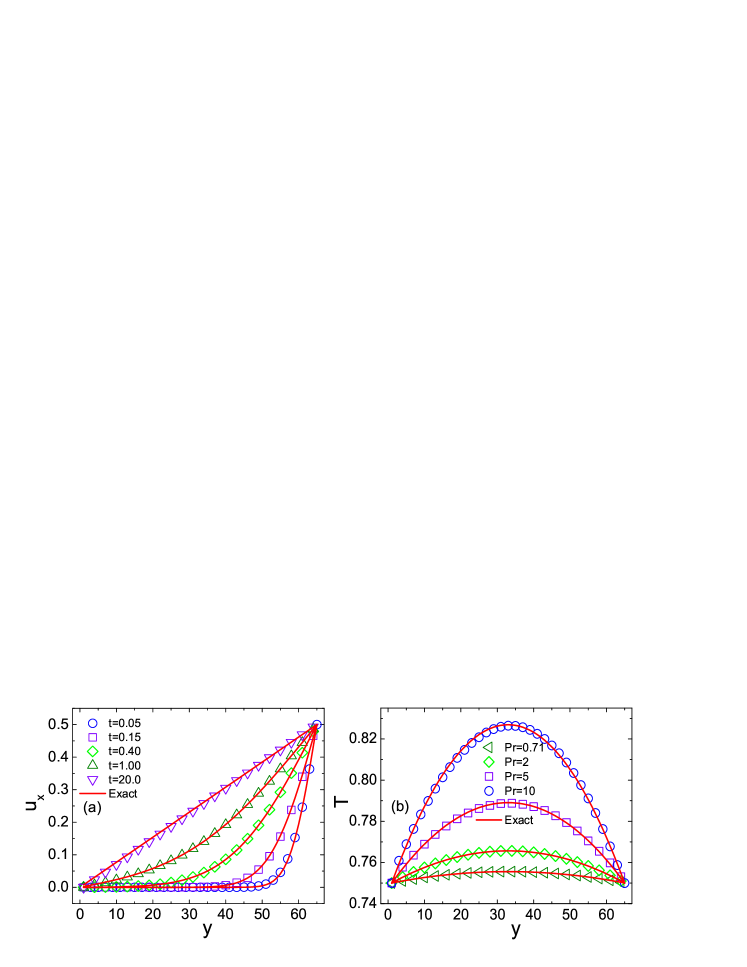
Figure 1: (a) Velocity profiles in unsteady Couette flow at characteristic times. (b) Temperature profiles in steady Couette flow for cases with various Prandtl numbers.

As a classical test where viscosity and heat transfer dominate, the thermal plane Couette flow is commonly applied to examine the ability of the DBM for simulating compressible flows with flexible Prandtl number 71 (71, 101, 102). For this problem considered, a viscous fluid flow between two infinite parallel flat plates separated by a constant distance of $H$, possesses the following initial conditions $(\rho,T,u_{x},u_{y})=(1.0,0.75,0.0,0.0)$. When the simulation starts, the top plate moves horizontally at the speed of $u_{0}=0.5$, while the bottom plate keeps stationary. Periodic BCs and nonequilibrium extrapolation scheme are applied in the $x$ and $y$ directions, respectively. Simulations have been carried out on a uniform mesh $N_{x}\times N_{y}=4\times 65$ with $\Delta x=\Delta y=3\times 10^{-3}$, $\tau=100\Delta t=10^{-3}$, $c=0.84$ and $\eta_{0}=2.0$. Figure 1(a) shows comparisons between the distributions of the horizontal velocity $u_{x}$ along the $y$-axis and the exact solutions at characteristic times $t=0.05$, $0.15$, $0.40$, $1.00$, $20.0$, respectively. To be noticed is that the simulation results agree well with the analytical solutions

$$u_{x}=\frac{y}{H}u_{0}+\frac{2}{\pi}u_{0}\overset{\infty}{\underset{n=1}{\sum}}[\frac{(-1)^{n}}{n}\exp(-n^{2}\pi^{2}\frac{\mu t}{\rho H^{2}})\sin(\frac{n\pi y}{H})]\text{,}$$ (6)

with $\mu=P\tau$ the viscosity coefficient. Figure 1(b) displays temperature profiles along the $y$-direction in the steady state for cases with different Prandtl numbers, where the following theoretical solutions are also exhibited for comparisons

$$T=T_{0}+\frac{\Pr}{2c_{p}}u_{0}^{2}\frac{y}{H}(1-\frac{y}{H})\text{.}$$ (7)

Here $T_{0}=0.75$ is the temperature of the top/bottom wall, $c_{p}=\gamma c_{v}$ is the specific heat at constant pressure with $\gamma=4/3$. As shown, the simulation results also match well with the corresponding analytical solutions, indicating the validity of the DBM in mimicking compressible flows with flexible Prandtl number.

III.2 Sod shock tube

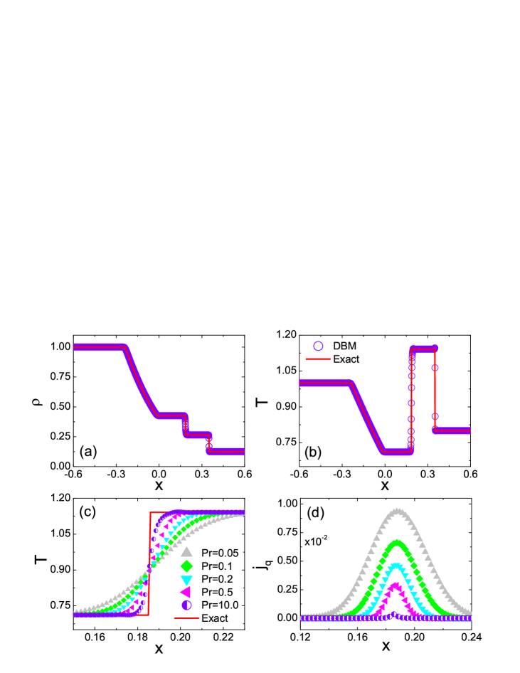
Figure 2: Profiles of density (a), temperature (b), local temperature (c) and heat flux (d) nearby the contact discontinuity with various Prandtl numbers calculated from DBM and Riemann solutions for the Sod shock tube, where $t=0.2$ and $\gamma=1.4$.

Due to the inclusion of rich and complex characteristic structures, the Sod shock tube problem is also a classical test used to verify the performance of models for compressible flow. The initial conditions are

$$\left\{\begin{array}[]{c}(\rho,T,u_{x},u_{y})|_{L}=(1.0,1.0,0.0,0.0),\\ (\rho,T,u_{x},u_{y})|_{R}=(0.125,0.8,0.0,0.0),\end{array}\right.$$ (8)

where subscripts “L" and “R" stand for macroscopic variables at the left and right sides of the discontinuity, respectively. In the $x$ and $y$ directions, we adopt the supersonic inflow and periodic BCs, respectively. Parameters are set to be $\Delta x=\Delta y=10^{-3}$, $\Delta t=5\times 10^{-5}$, $c=1.06$, $\eta_{0}=1.5$, $\gamma=1.4$, $N_{x}\times N_{y}=2000\times 4$. The relaxation time $\tau$ is fixed at $5\times 10^{-5}$ for all simulations. Shown in Fig. 2 are the computed profiles of density, temperature, local temperature and heat flux nearby the contact discontinuity for cases with various Prandtl numbers at $t=0.2$, where solid lines indicate Riemann solutions. From the top two subgraphs, it is clear that the left-propagating rarefaction wave, the right-propagating shock wave and the contact discontinuity have been exactly captured with severely curtailed numerical dissipation. Enlargement of the local part containing shock wave manifests that the shock wave only spreads over three to four grid cells. For a fixed viscosity, the increase in Prandtl number leads to the decrease in heat conductivity. Figures 2(c)-(d) inform us that heat conduction smoothes the temperature profile, reduces the temperature gradient, but enlarges the amplitude of heat flux and extends the nonequilibrium region.

III.3 Modified Colella’s explosion wave test

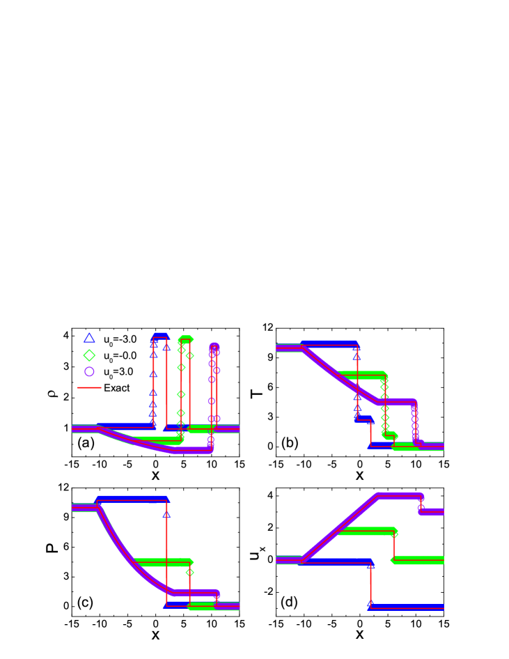
Figure 3: Profiles of density (a), temperature (b), pressure (c) and velocity (d) with various initial conditions calculated from DBM and Riemann solutions for the modified Colella’s shock tube, where $t=2.5$, $\gamma=5/3$ and $\Pr=0.71$.

To further examine the robustness and effectiveness of the model for compressible flows with high Mach number, we construct modified Colella’s explosion wave tests with weaker temperature discontinuity but stronger velocity discontinuity

$$\left\{\begin{array}[]{c}(\rho,T,u_{x},u_{y})|_{L}=(1.0,10.0,0.0,0.0),\\ (\rho,T,u_{x},u_{y})|_{R}=(1.0,1/30,u_{0},0.0).\end{array}\right.$$ (9)

Comparisons between simulation results and the exact solutions at $t=2.5$ are plotted in Fig. 3, with $u_{0}=-3.0$, $0.0$, and $3.0$. Parameters used here are $\Delta x=\Delta y=10^{-2}$, $\Delta t=5\times 10^{-5}$, $\tau=2\times 10^{-5}$, $c=2.06$, $\eta_{0}=20.0$, $\gamma=5/3$, $N_{x}\times N_{y}=4000\times 2$. The simulation results agree excellently with Riemann solutions for each case. Moreover, the shock wave and contact discontinuity are captured stably without overshoots or spurious oscillations. Successful simulation of this aggressive tests manifests that the proposed model is robust, accurate and applicable to compressible flows with high-Mach-number ( $Ma=12.7$ for case with $u_{0}=3.0$), high temperature and pressure ratios (up to $300$).

IV Effects of viscosity and heat conduction on KHI

In this section, we conduct a parametric study to evaluate the effects of viscosity and heat conduction on the formation and evolution of the KHI. Both the HNE and TNE manifestations provided by DBM, as well as morphological characterizations described by Minkowski measures, have been extracted to analyze and understand the complex configurations and nonequilibrium processes. For all simulations, the whole two dimensional calculation domain corresponds to a rectangle with length $L_{x}=1.8$ and height $L_{y}=0.6$, divided into $600\times 200$ grid cells.

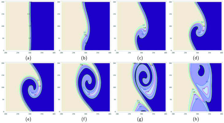
Figure 4: Time series of the density patterns simulated via the DBM, where $t=0.1$ in (a), $t=0.7$ in (b), $t=1.0$ in (c), $t=1.2$ in (d), $t=1.5$ in (e), $t=2.0$ in (f), $t=2.45$ in (g), and $t=2.85$ in (h). Only the part with $x$ in the range $[200:400]$ of the full grid is shown. From purple to light brown, the density increases.

IV.1 Density patterns, nonequilibrium and morphological characterizations

The initial configurations of our simulations are functions of $x$, read

$$\rho(x)=\frac{{\rho_{L}+\rho_{R}}}{2}-\frac{{\rho_{L}-\rho_{R}}}{2}\tanh(\frac{x-L_{x}/2}{{D_{\rho}}})\text{,}$$ (10)

$$u_{y}(x)=\frac{{u_{yL}+u_{yR}}}{2}-\frac{{u_{yL}-u_{yR}}}{2}\tanh(\frac{x-L_{x}/2}{{D_{u}}})\text{,}$$ (11)

$$P_{L}=P_{R}=P\text{,}$$ (12)

where $D_{\rho}=4$ ($D_{u}=4$) indicates the width of density (velocity) transition layer. $\rho_{L}=2.4$ ($\rho_{R}=0.6$) is the density away from the interface of the left (right) fluid. $u_{yL}=-u_{yR}=0.5$ stands for the fluid owning opposite vertical velocities in the two halves, while having homogeneous pressure $P=1.2$. In the absence of any perturbation, the configuration maintains in mechanical equilibrium. To trigger the KH rollup, we introduce a small velocity perturbation in the $x$ direction as

$$u_{x}(x)=u_{0}\sin(ky)\exp(-2\pi|x-L_{x}/2|)\text{,}$$ (13)

where $u_{0}=20\Delta x$ denotes the amplitude of the initial perturbation and $k=2\pi/L_{y}$ is the wave number of the initial perturbation. Periodic BCs are applied in the $y$ direction and outflow boundary conditions are adopted in the $x$ direction. The time step is set to be as small as $\Delta t=10^{-5}$ to reduce the numerical dissipation. The remaining parameters are $c=1.2$, $\eta_{0}=200$, $\tau=2\times 10^{-4}$ and $\gamma=5/3$.

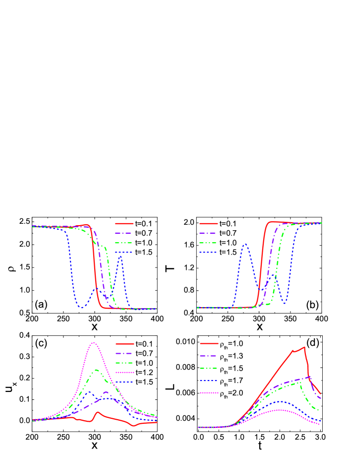
Figure 5: Profiles of density (a), temperature (b) and velocity(c) along the horizontal centerline $y=L_{y}/2$ at various times, and time evolutions of boundary length $L$ (d) for various density thresholds $\rho_{\text{th}}$.

Figure 4 shows time series of density patterns with five contour lines during the evolution of KHI. From it, four distinct evolutionary regimes, i.e., the oscillatory regime, the linear growth stage, the nonlinear growth stage with highly rolled-up vortices, and finally, a turbulent phase with nonregular structures, can be distinguished. Specifically, in the first stage [see panel (a)], the continuous interface between the two layers begins wiggling under the action of the initial perturbation and the velocity shear. After such a transient period, the perturbation grows exponentially and results in a sinuous structure dominating in panels (b)-(d). In the subsequent nonlinear phase, a roughly circular vortex is formed at the expense of the vortex in the braid regions [see panel (e)]. After saturation, the vortex is further stretched in the $y$ direction and becomes elliptical as shown in panel (f). In the final stage, the normal vortex structure collapses and the mixing layer approaches the boundary, marking that the system proceeds to the turbulent stage. Moreover, it is observed that the position of the mixing layer moves toward the $x$ direction from the center of the computational domain, which enhances the transfer of fluids from the dense to the tenuous region.

To further understand the development of the vortex or the mixing layer, in Fig. 5, we illustrate the density, temperature and velocity profiles along the horizontal centerline $y=L_{y}/2$ at representative times. The density and temperature profiles vary from being smooth (tangent profiles) to being irregular. The width of the mixing layer and the amplitude of the oscillation increase with time, due to the mass-momentum-energy transport from the dense (hot) to the rarefactive (cold) regions, see the crest at $x=340$ ($x=277$) in the density (temperature) profile at $t=1.5$ and the fully developed horizontal velocity $u_{x}(x)$, which attains a maximum at $t=1.2$ (roughly $70\%$ of $u_{yL}$), before decreasing monotonically to zero.

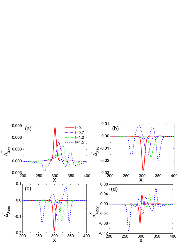
Figure 6: Nonequilibrium measures $\Delta_{2xy}^{*}$ (a), $\Delta_{31x}^{*}$ (b), $\Delta_{3xxx}^{*}$ (c), and $\Delta_{42xy}^{*}$ (d) along the horizontal centerline $y=L_{y}/2$ at various times.

Next, the Minkowski measures are presented to extract information from the complex patterns displayed in Fig. 4. According to the morphological analysis, a physical field $\Theta(\mathbf{r},t)$ of interest can be condensed as two kinds of characteristic regimes: the white (with $\Theta>\Theta_{\text{th}}$) and the black (with $\Theta<\Theta_{\text{th}}$), where $\Theta_{\text{th}}$ is a threshold of $\Theta$. For such a Turing pattern, a general theorem of integral geometry states that all the properties of a $d$-dimensional convex set satisfying motion invariance and additivity are contained in $d+1$ Minkowski measures. To be specific, for a two dimensional density field, the three Minkowski measures are the total fractional area $A$ of the high-density regimes, the boundary length $L$ between the high- and low-density regimes per unit area, and the Euler characteristic $\chi$ per unit area. Figure 5(d) depicts the time evolutions of boundary length $L$ for various density thresholds $\rho_{\text{th}}$, in a log-linear scale. As shown, these curves behave qualitatively similar and can be roughly divided into four stages, marked individually by red arrows for $L(t)$ curve with $\rho_{\text{th}}$ equaling to the averaged density. The first stage corresponds to the time delay for observing evident KH billows. Still no notable instability occurs for all the density thresholds. Afterwards, $L$ increases exponentially till $t=1.5$, followed by a slow increase to attain the peak at about $t=2.5$; whereafter decreases abruptly, especially for cases with smaller thresholds. The first increase and the subsequent decrease in $L$ are due to the growth, formation, and deformation of the KH rolls from small fluctuations undergoing the linear and nonlinear stages, and the finally coalesce of the high- and low-density domains by the secondary instabilities that induces vortex breakup during the oversaturated turbulent stage, respectively.

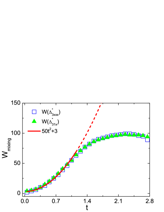
Figure 7: Widths of the mixing layers obtained from interface-tracking technique based on the nonequilibrium measures $\Delta_{3xxx}^{*}$ and $\Delta_{31x}^{*}$.

Besides being able to recover hydrodynamic equations at various levels (Navier-Stokes, Burnett, super-Burnett, etc.), DBM also provides us a set of handy, effective and efficient tools to describe, measure, and analyze the TNE behaviors, by calculating the difference between the non-conserved central kinetic moments of discrete distribution function and DEDF, $\bm{\Delta}_{m,n}^{\ast}=\mathbf{M}_{m,n}^{\ast}(f_{i})-\mathbf{M}_{m,n}^{\ast}(f_{i}^{(0)})=\sum\nolimits_{i}(f_{i}-f_{i}^{(0)})(\frac{v_{i}^{\ast 2}+\eta_{i}^{2}}{2})^{\frac{m-n}{2}}\mathbf{v}_{i}^{\ast n}$, with $\mathbf{v}_{i}^{\ast}=\mathbf{v}_{i}-\mathbf{u}$ the thermal velocity. Figure 6 qualitatively portrays the typical nonequilibrium manifestations $\Delta_{2xy}^{\ast}$, $\Delta_{3,1x}^{\ast}$, $\Delta_{3xxx}^{\ast}$, and $\Delta_{4,2xy}^{\ast}$ during the development of KHI. The following features can be obtained: (i) For an ideal gas system, gradient force acts as the unique driving force for TNE and HNE. So, the TNE quantities are mostly around the interface where the gradients of macroscopic quantities are pronounced and exactly attain their local maxima (minima) at the points of the maxima ($\bm{\nabla}\rho,\bm{\nabla}T,\bm{\nabla}\bm{u})_{\text{max}}$; while approach zero at positions far away from the interface or at peaks (valleys) with vanishing gradients. For example, at the peak ($x=277$) and valley ($x=340$) of $T(x,L_{y}/2)$ at the time $t=1.5$ [see Fig. 5(b)], $\Delta_{3,1x}^{\ast}$ is nearly in its thermodynamic equilibrium [see Fig. 6(b)]. At the two sides of the peak (valley), the system deviates from its equilibrium in opposite directions. (ii) For each kind of TNE quantity, the shear component, such as $\Delta_{2xy}^{\ast}$ and $\Delta_{4,2xy}^{\ast}$, or the flux in the $x$ direction, such as $\Delta_{3,1x}^{\ast}$ and $\Delta_{3xxx}^{\ast}$, own the largest amplitudes (other components such as $\Delta_{2xx}^{\ast}$, $\Delta_{3,1y}^{\ast}$, $\Delta_{3xxy}^{\ast}$, etc., are not shown here). Behaviors of TNE measures can be interpreted as follows. Physically, $\bm{\Delta}_{2}^{\ast}$ and $\bm{\Delta}_{3,1}^{\ast}$ correspond to more generalized viscous stress and heat flux, respectively; $\bm{\Delta}_{3}^{\ast}$ and $\bm{\Delta}_{4,2}^{\ast}$ correspond to more generalized fluxes of viscous stress and heat flux, respectively. Essentially, KHI is a kind of shearing instability through which mass-momentum-energy transfer through the initial interface, resulting in remarkable shear-induced nonequilibrium and transporting nonequilibrium. (iii) For any TNE manifestation, although the nonequilibrium amplitude evolves complicatedly, the nonequilibrium region (NER) extends with evolution on account of the KHI-induced mixing process. The width of the NER justly corresponds to the width of the mixing layers $w_{\text{mixing}}$. Therefore, we present here an interface-tracking method through tracking the leftmost and the rightmost positions with $|\bm{\Delta}_{m,n}^{\ast}|\geq|\bm{\Delta}_{m,n}^{\ast}|_{\text{th}}$, where $|\bm{\Delta}_{m,n}^{\ast}|_{\text{th}}$ is a threshold of $|\bm{\Delta}_{m,n}^{\ast}|$.

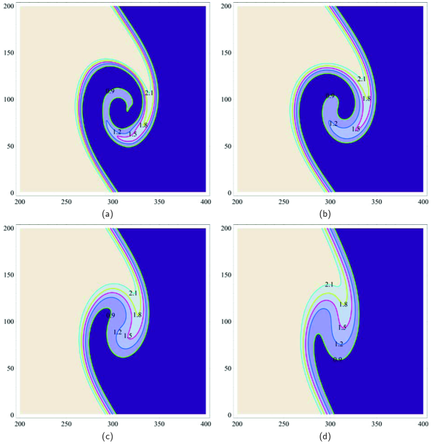
Figure 8: Vortices in the mixing layer as a function of viscosity at $t=1.4$, where $\tau=10^{-5},10^{-4},5\times 10^{-4}$ and $10^{-3}$ in (a), (b), (c) and (d), respectively. Only the part with $x$ in the range $[200:400]$ of the full grid is shown. From purple to light brown, the density increases.

Figure 9: Time evolution of the logarithm of the perturbed peak kinetic energy $E_{x\text{-max}}$ for cases with various viscosities, where solid lines represent the linear fits to the initial linear growth regimes (a). Linear growth rate as a function of $\tau$ (b). Saturation time $t_{\text{sat}}$ (c) and peak perturbed kinetic energy (d) for cases with various viscosities.

Figure 10: Effects of viscosity on nonequilibrium measure $\Delta_{2xy}^{*}$ (a) and high velocity area fraction $A$ for $|u|_{\text{th}}=0.2$ (c). Effects of viscosity on the non-dimensionalized nonequilibrium intensity $D^{*}$ (b) and boundary length $L$ for $\rho_{\text{th}}=1.80$ (d).

Essentially, the mixing zone width and its growth rate are of great significance in the study of the hydrodynamic instability and turbulent mixing 29 (29, 103, 104, 105, 106, 107, 108). The time evolution of $w_{\text{mixing}}$, revealing the mixing extent and efficiency, is an important parameter to quantitatively study the development of KHI. Usually, for incompressible KHI, the measurement is readily performed by tracing the constant density. Nevertheless, in the compressible case, how to measure the mixing layer remains a thorny problem. The interface-tracking approach based on TNE measures may shed some light on identification, labelling and extraction of characteristic structures from complex physical fields. To elaborate on this point, Fig. 7 exhibits temporal evolution of the mixing layers thickness by tracking boundaries of $\Delta_{3xxx}^{*}$ and $\Delta_{31x}^{*}$. It is evident that, although acquired from different TNE measures, $w_{\text{mixing}}$ approximately overlap with each other, manifesting that TNE quantities have been coupled with each other. In other words, gradient in one quantity, say density gradient, can stimulate gradients in other quantities, say velocity and temperature gradients. The non-monotonic $w_{\text{mixing}}$ can be approximately divided into four stages, i.e., a drastic increase until $t=1.4$, a mild increase, a plateau, and a steep decrease from about $t=2.5$ which are basically consistent with scenarios in Figs. 4 and 5. Moreover, it is found that, when $t<1.4$, $w_{\text{mixing}}$ dramatically increase with $t$ according the the following way

$$w_{\text{mixing}}=At^{2}+B\text{,}$$ (14)

with $A=50$ and $B=3$, which is substantially different from the the Richtmyer-Meshkov instability 105 (105).

IV.2 Effects of viscosity

Here, focus is on how and to what extent viscosity affects the dynamic patterns, nonequilibrium and morphological features. To this end, we have performed comparative calculations with fixed thermal conductivity $\kappa_{T}=1.2\times 10^{-3}$, but varying viscosity coefficients $\mu$ through changing relaxation time $\tau$ over two decades. Figure 8 shows density maps for $\tau=10^{-5},10^{-4},5\times 10^{-4}$ and $10^{-3}$ with five contour lines at $t=1.4$, respectively. Apparently, the striking differences in density patters demonstrate that the evolution of KHI depends on viscosity strongly. For fixed initial conditions and model parameters, the larger the viscosity, the weaker the KHI, and the later the vortex appears. The viscous force persistently extracts perturbation kinetic energy from the fluids and erases progressively the small substructures. Therefore, we see from the top row that, at lower viscosity, largely rolled billows consisting of more windings, diverse length scales, and very sharp density interfaces, appear. Larger viscosity delays the formation of the instability and inhibits the onset completely in cases with extremely high values. As observed in the bottom row of Fig. 8, cusps, instead of roll-up motions, forms. Figure 8 indicates that the fluid viscosity tends to suppress and limit the growth of the KHI.

The stabilizing effects of viscosity can be further confirmed by the temporal evolution of logarithm of the perturbed peak kinetic energy $E_{x\text{-max}}(t)$ for cases with various $\tau$ [see Fig. 9(a)]. For each case, $E_{x\text{-max}}(t)$ experiences four stages as well, in accordance with Figs. 4, 5 and 7. After an initial settling period, it increases exponentially during the linear phase, until the reach of the saturation stage with the saturation energy $E_{\text{sat}}$. $E_{\text{sat}}$, determined as the first peak amplitude in $E_{x\text{-max}}(t)$ arrived at time $t_{\text{sat}}$, can be used to measure the suppression level by viscosity and the non-linear evolution of KHI. After that, we also see the finite-amplitude oscillation in $E_{x\text{-max}}(t)$, owing to the generation and development of the subharmonic modes. Subsequently, $E_{x\text{-max}}(t)$ decreases almost exponentially towards the initial perturbed level ($t>1.8$, not shown here). The linear growth rate $\gamma$ can be obtained from the slope of the linear function fitted to the growth phase, shown by the solid lines. $E_{x\text{-max}}(t)$ represents the interacting strength of two different fluids. At the same moment, the larger the viscosity, the lower the perturbed peak kinetic energy, manifesting hindering effects of viscosity on KHI. Figure 9 demonstrates that the viscosity effects are threefold: significantly refrain both the linear growth rate $\gamma$ and the saturation energy $E_{\text{sat}}$, prominently prolong the duration of the linear growth stage $t_{\text{linear}}$ or postpone the saturation time $t_{\text{sat}}$, approximately in the following ways:

$$\gamma=a-b\tau^{0.3}\text{,}$$ (15)

$$\ln E_{\text{sat}}=c-d\tau\text{,}$$ (16)

$$t_{\text{sat}}=e+f\tau^{0.5}\text{,}$$ (17)

with $a=4.90$, $b=30.30$, $c=-1.65$, $d=2402.79$, $e=0.94$, and $f=30.73$, respectively. In the classical case where Euler equations dominate, the linear growth rate reads $\gamma_{c}=k\sqrt{\rho_{1}\rho_{2}}\Delta v/(\rho_{1}+\rho_{2})$ 47 (47, 48), where $\Delta v$ is the shear velocity difference. Higher viscous dissipation hampers the development of $\Delta v$ and removes more kinetic energy gained from the shear velocity, resulting in a smaller growth rate, a lower saturation energy, and a longer linear growth stage.

Figure 10(a) reveals how viscosity affects the shear TNE component $\Delta_{2xy}^{*}$ along the line $y=N_{y}/2$ at $t=0.6$. To be seen is that, viscosity enhances both the local and global nonequilibrium strengths, broadens the nonequilibrium region. For case with $\tau=10^{-4}$, the nonequilibrium region is confined to $[294:322]$ and the nonequilibrium amplitude is about $0.003$; while for case with $\tau=8\times 10^{-4}$, the counterparts are $[260:342]$ and $0.0127$, respectively. Moreover, we find that, although $\Delta_{2xy}^{*}$ is proportional to $\tau$, the amplitudes of $\Delta_{2xy}^{*}$ do not increase with $\tau$ linearly. This is because, the relaxation time $\tau$ plays opposite roles in both the thermodynamical and hydrodynamical aspects. Thermodynamically, it maintains the system in a far-from-equilibrium state through retaining the macroscopic quantity gradients to high levels. But hydrodynamically, it extends the density profile, reduces the temperature gradient, etc., then makes the system deviate less from its thermodynamic equilibrium. Effects of viscosity on high-velocity area fraction $A$ for $u_{\text{th}}=0.2$ are shown in Fig. 10(c). These curves behave qualitatively similar and can be divided into three stages, corresponding to the time delay stage with nearly zero value of $A$, the rapid increase and the subsequent decrease in $A$. Asides from similarity, the distinct differences resulted from various $\tau$ are as below. The larger the viscosity, the longer the time delay for observable KHI under fixed velocity threshold, as well as the smaller the slope and amplitude of $A(t)$ curve in the second stage. In fact, slopes of $A(t)$ curves correspond approximately to the evolution speed of KHI. From this point of view, the instability is remarkably decelerated by viscosity.

Figure 10(b) exhibits effects of viscosity on the non-dimensionalized nonequilibrium intensity $D$ and boundary length $L$ for $\rho_{\text{th}}=1.80$ [panel (d)]. Here $D$ is defined as

$$D=\frac{1}{L_{x}L_{y}}\int_{0}^{L_{x}}\int_{0}^{L_{y}}(\frac{\bm{\Delta}_{2}^{\ast 2}}{T^{2}}+\frac{\bm{\Delta}_{3,1}^{\ast 2}}{T^{3}}+\frac{\bm{\Delta}_{3}^{\ast 2}}{T^{3}}+\frac{\bm{\Delta}_{4,2}^{\ast 2}}{T^{4}})^{1/2}dxdy\text{,}$$ (18)

where $D=0$ in the thermodynamic equilibrium state and $D>0$ in the thermodynamic nonequilibrium state. Clearly, for a fixed $\tau$, $D(t)$ increases to its maximum then decreases slowly. For cases with different $\tau$, all $D(t)$ curves increase with $\tau$ and approach their maxima at about the same time $t=2.0$. The evolutions of $D(t)$ and $L(t)$ present considerably high degree of correlation. For instance, $L(t)$ also increases with $\tau$ and behaves the first increase and latter decrease way as $D(t)$. Once again, all $L(t)$ curves reach their peaks also at the same moment with $D(t)$ for cases with various $\tau$. Physically, the dominating part of non-dimensionalized nonequilibrium intensity $D(t)$ is a combination of products of hydrodynamic quantities gradients ($\bm{\nabla}\rho$, $\bm{\nabla}\mathbf{u}$ and $\bm{\nabla}T$) and $\tau$. Therefore, for a single curve, a larger boundary length $L(t)$ corresponds to greater density gradients and more intense nonequilibrium extent. Owing to the violent resistance effects of $\tau$ on KHI, we mention that, the smaller the $\tau$, the larger the $L(t)$. Oppositely, the larger the $L(t)$, the weaker the $D(t)$, indicating the leading role of $\tau$ versus ($\bm{\nabla}\rho$, $\bm{\nabla}\mathbf{u}$ and $\bm{\nabla}T$). Comparisons between panels (b) and (d) show that the evolutions of TNE intensity and boundary length present high correlation and attain their maxima almost simultaneously.

Figure 11: Widths of the mixing layers for cases with various viscosities obtained from evolutions of $\Delta_{3xxx}^{*}$.

Figure 11 displays widths of the mixing layers $w_{\text{mixing}}$ for several cases with different viscosities obtained from the interface-tracking technique based on TNE measure $\Delta_{3xxx}^{*}$. As shown, for different cases, evolutions of $w_{\text{mixing}}$ are self-similar and behave qualitatively quite similar as boundary length $L$ [Fig. 10(d)]. Nevertheless, different relaxation times $\tau$ generate different $w_{\text{mixing}}$. The larger the $\tau$, the narrower the $w_{\text{mixing}}$. Figure 11 quantitatively reflects the hindering effects of viscosity on the onset and development of KHI.

IV.3 Effects of heat conduction

Figure 12: Vortices in the mixing layer as a function of heat conduction at $t=1.4$, where $\kappa_{T}=1.5\times 10^{-4},1.5\times 10^{-3},6\times 10^{-3}$ and $1.5\times 10^{-2}$ in (a), (b), (c) and (d), respectively. Only the part with $x$ in the range $[200:400]$ of the full grid is shown. From purple to light brown, the density increases.

Effects of heat conduction are tentatively analyzed in a similar way with fixed relaxation time $\tau=10^{-4}$ and various thermal conductivities $\kappa_{T}$. Shown in Fig. 12 are the typical density patterns at $t=1.4$ for cases with $\kappa_{T}=1.5\times 10^{-4},1.5\times 10^{-3},6\times 10^{-3}$ and $1.5\times 10^{-2}$, respectively. The KH structure changes considerably as the heat conduction varies. For case with smaller $\kappa_{T}$, the cat’s eye structure with spiral arm has been observed from the density fields. While, at larger $\kappa_{T}$, the initial disturbance merely develops into brawny cusp that tentatively whirls across the transition layer. Meanwhile, the mixing layer is thickening and the higher order harmonic is refraining by thermal diffusion, which results in single and larger scale configuration. Roughly speaking, the heat conduction stabilize the KHI by suppressing the growth of the initial perturbation and the appearance of the higher order harmonics.

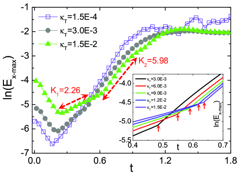
Figure 13: Time evolution of the perturbed peak kinetic energies $E_{x\text{-max}}$ in a ln-linear scale for cases with various heat conductivities $\kappa_{T}$. Evolution of $E_{x\text{-max}}(t)$ during the stage $0.4<t<0.7$ has been shown in the inset, where red arrows pointing towards the inflection points.

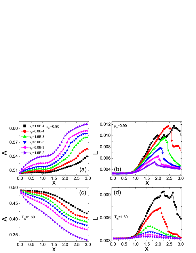
Figure 14: Effects of heat conduction on high density area fraction $A$ (a) and high density boundary length $L$ (b) for $\rho_{\text{th}}=0.90$. Effects of heat conduction on high temperature area fraction $A$ (c) and high temperature boundary length $L$ (d) for $T_{\text{th}}=1.60$.

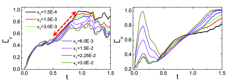
Figure 15: Temporal evolutions of the average widths of density (a) and longitudinal velocity (b) transition layers.

Figure 13 gives time evolution of the perturbed peak kinetic energies $E_{x\text{-max}}$ in a ln-linear scale for cases with various $\kappa_{T}$. Generally speaking, $\kappa_{T}$ reduces the linear growth rate. Nevertheless, the stabilizing effects are not as obvious as viscosity, moreover, become less important for larger $\kappa_{T}$, manifested by the little differences in slopes of $E_{x\text{-max}}(t)$ and the nearly identical saturation kinetic energy $E_{\text{sat}}$ for diverse cases. Meanwhile we mention a significant effect of $\kappa_{T}$, for large enough $\kappa_{T}$, say $\kappa_{T}=1.5\times 10^{-2}$, after the initial transient period and before the vortex has been well formed, the evolution of $E_{x\text{-max}}(t)$ undergoes two linear stages with distinct slopes. To highlight this point, evolution of $E_{x\text{-max}}(t)$ during the stage $0.4<t<0.7$ has been shown in the inset, where red arrows pointing towards the inflection points. The larger the heat conductivity, the later the inflection point appears, the smaller the perturbed peak kinetic energy before the inflection point, but the greater the perturbed peak kinetic energy after the inflection point. Behaviors of $E_{x\text{-max}}(t)$ at large $\kappa_{T}$ demonstrate that the heat conduction effects are not monotonic: first refrain but favor the evolution afterwards.

To further clarify effects of heat conduction, we illustrate the morphological features of density and temperature fields in Fig. 14. For all cases, the high density area fraction $A(t)$ and boundary length $L(t)$ for $\rho_{\text{th}}=0.90$ increase with time due to the viscous heating, the timely heat diffusion, and the appearance of new interface between fluids of different densities. Nevertheless, effects of heat conduction on $A(t)$ and $L(t)$ are completely opposite. At the same moment, the larger the $\kappa_{T}$, the higher the $A$, but the lower the $L$. This indicates that the thermal diffusion primarily promotes the translational motion of the interface and suppresses the curl of the initial perturbation. The slope of $L(t)$ clearly represents the development rate of KHI. Once again, we conclude the KHI is decelerated by heat conduction. The $A(t)$ and $L(t)$ curves for temperature field at threshold $T_{\text{th}}=1.60$ are shown in the bottom row of Fig. 14. Similar conclusion can be acquired from $L(t)$ curves for temperature field. But for $A(t)$ curves, we see that heat conduction lowers the proportion with temperature $T>T_{\text{th}}$ owing to the larger $\kappa_{T}$ that makes the system approach thermodynamical equilibrium quickly.

To interpret behaviors of $E_{x\text{-max}}(t)$ at large $\kappa_{T}$, in Fig. 15, we monitor the temporal histories of the normalized widths of density and velocity transition layers, refereed to as $\bar{L}_{\rho}$ and $\bar{L}_{u}$, respectively. Therein, $\bar{L}_{\rho}$ is defined as

$$\bar{L}_{\rho}=\frac{1}{L_{\rho}^{\text{max}}}\frac{1}{L_{x}L_{y}}\int_{0}^{L_{x}}\int_{0}^{L_{y}}\rho(|\frac{\partial\rho}{\partial x}|^{-2}+|\frac{\partial\rho}{\partial y}|^{-2})^{1/2}dxdy$$ (19)

when $|\frac{\partial\rho}{\partial x}|>0.1$ and $|\frac{\partial\rho}{\partial y}|>0.1$; otherwise $\bar{L}_{\rho}=0$. $\bar{L}_{u}$ is defined similarly. As can be seen, for all $\bar{L}_{\rho}(t)$ curves, when $t<0.25$, they increase sharply and overlap with each other, representing the initial relaxation stage where the violent temperature gradients attempt to initiate the instability through thickening the density transition layer. Compared to $\bar{L}_{\rho}(t)$, $\bar{L}_{u}(t)$ grows more steeply, impetuously and inconsistently during this period. As a result, significant differences appear in $\bar{L}_{u}(t)$. For example, $\bar{L}_{u}(t)$ for $\kappa_{T}=3\times 10^{-2}$ is about 3 times wider than that for $\kappa_{T}=1.5\times 10^{-4}$ at $t=0.14$. The wider transition layer $\bar{L}_{u}$ effectively decreases the local shear velocity difference $\Delta v$ and results in a smaller linear growth rate in $E_{x-\text{max}}(t)$. This can be seen more clearly from the square of the linear growth rate for the classical case 48 (48), $\gamma_{c}^{2}=k^{2}\rho_{1}\rho_{2}(v_{1}-v_{2})^{2}/(\rho_{1}+\rho_{2})^{2}\propto(1-A^{2})\Delta v^{2}$, where $A=(\rho_{1}-\rho_{2})/(\rho_{1}+\rho_{2})$ is the Atwood number.

On the other hand, when $0.25<t<1.0$, all $\bar{L}_{\rho}(t)$ curves further increase with time, but decreases prominently with $\kappa_{T}$, until the arrivals of the slightly oscillating platforms with various heights (labelled by red line with double-headed arrows). The persistent and notable growth in $\bar{L}_{\rho}$, gives rise to a wider density transition zone that reduces the effective Atwood number around the interface. Therefore, in the process of exchanging momentum along the direction normal to the interface, the perturbation obtains energy easily from the shear layers than in cases with steeper interfaces or with higher density ratios. Meanwhile, $\bar{L}_{u}$ slide to their valleys at about $t=0.5$. Consequently, the limited $\bar{L}_{u}$ and the fully developed $\bar{L}_{\rho}$ advance the instability enormously, and give rise to the second and steeper increase in $E_{x-\text{max}}(t)$.

V Conclusions and remarks

An efficient and easily implementable discrete Boltzmann model is proposed to systematically study the viscosity and heat conduction effects on the onset and growth of compressible Kelvin-Hemholtz instability (KHI). Both thermodynamic nonequilibrium (TNE) and morphological characterizations are extracted, for the first time, to analyze and understand the configurations and the kinetic processes.

The findings are as below. On the technical side, two novel approaches, independent from each other, are presented to quantitatively feature the evolution of KHI. One is to determine the thickness of mixing layers via tracking the distributions and evolutions of the TNE measures. The other is to access the growth rate of KHI via the slopes of Minkowski measures. On the physical side, it is interesting to find that the time histories of width of mixing layer, TNE intensity, and boundary length between the high and low macroscopic quantity regimes show high correlation and attain their maxima simultaneously. The effects of viscosity are twofold. One is to stabilize the KHI through reducing the linear growth rate, prolonging the duration of the linear growth stage, and suppressing the hydrodynamic velocity and the perturbed peak kinetic energy. The other is to enhance both the local and global nonequilibrium strengths via enlarging the relaxation time and broadening the nonequilibrium region, respectively. Contrary to the monotonically inhibiting effects of viscosity, the simulations reveal that the heat conduction effects refrain at first then accelerate the evolution afterwards. This is because heat conduction extends both the widths of density and velocity transition layers simultaneously. While the two kinds of widths act oppositely on the evolution of KHI. During the first period, the growing velocity transition layer dominates the evolution; After that, the persistently increasing density transition layer together with the temporarily decreasing velocity transition layer dominates the evolution jointly.

Although this work focus on two-dimensional case, the introduced morphological analysis method and the developed interface-capturing technique based on TNE measures, can be applied to pick up information from three-dimensional physical fields. The nonequilibrium and morphological characterizations of three-dimensional KHI in multiphase flows and compressible flows deviating far away from thermodynamic equilibrium deserve further study and are currently in progress.

References

- (1) S. Chandrasekhar, Hydrodynamic and Hydromagnetic Stability (Oxford University, London, 1961)
- (2) W. D. Smyth and J. N. Moum, Anisotropy of turbulence in stably stratified mixing layers, Phys. Fluids 12, 1327 (2000)
- (3) Y. Matsumoto and M. Hoshino, Onset of turbulence induced by a Kelvin-Helmholtz vortex, Geophys. Res. Lett. 31, L02807 (2004)
- (4) O. Berné and Y. Matsumoto, The Kelvin-Helmholtz instability in Orion: a source of turbulence and chemical mixing, Astrophys. J. Lett. 761, L4 (2012)
- (5) Z. Xia, Y. Shi, and Y. Zhao, Assessment of the shear-improved Smagorinsky model in laminar-turbulent transitional channel flow, J. Turbul. 16, 925 (2015)
- (6) Z. Xia, Y. Shi, and S. Chen, Direct numerical simulation of turbulent channel flow with spanwise rotation, J. Fluid Mech. 788, 42 (2016)
- (7) Z. Xia, Y. Shi, Q. Cai, M. Wan, and S. Chen, Multiple states in turbulent plane Couette flow with spanwise rotation, J. Fluid Mech. 837, 477 (2018)
- (8) R. P. Drake, High-Energy-Density Physics: Fundamentals, Inertial Fusion and Experimental Astrophysics (Springer, New York, 2006)
- (9) M. T. Montgomery, V. A. Vladimirov, and P. V. Denissenko, An experimental study on hurricane mesovortices, J. Fluid Mech. 471, 1 (2002)
- (10) K. Wada and J. Koda, Instabilities of spiral shocks-I. Onset of wiggle instability and its mechanism, Mon. Not. R. Astron. Soc. 349, 270 (2004)
- (11) S. N. Borovikov and N. V. Pogorelov, Voyager 1 near the heliopause, Astrophys. J. Lett. 783, L16 (2014)
- (12) K. Avinash, G. P. Zank, B. Dasgupta, and S. Bhadoria, Instability of the heliopause driven by charge exchange interactions, Astrophys. J. Lett. 791, 102 (2014)
- (13) H. Hasegawa, M. Fujimoto, T. D. Phan, H. Rème, A. Balogh, M. W. Dunlop, C. Hashimoto, and R. TanDokoro, Transport of solar wind into Earth’s magnetosphere through rolled-up Kelvin-Helmholtz vortices, Nature 430, 755 (2004)
- (14) C. Foullon, E. Verwichte, V. M. Nakariakov, K. Nykyri, and C. J. Farrugia, Magnetic Kelvin-Helmholtz instability at the Sun, Astrophys. J. Lett. 729, L8 (2011)
- (15) X. T. He and W. Y. Zhang, Inertial fusion research in China, Eur. Phys. J. D 44, 227 (2007)
- (16) L. Wang, W. Ye, X. He, J. Wu, Z. Fan, C. Xue, H. Guo, W. Miao, Y. Yuan, J. Dong, G. Jia, J. Zhang, Y. Li, J. Liu, M. Wang, Y. Ding, and W. Zhang, Theoretical and simulation research of hydrodynamic instabilities in inertial-confinement fusion implosions, Sci. China-Phys. Mech. Astron. 60, 055201 (2017)
- (17) M. Vandenboomgaerde, M. Bonnefille, and P. Gauthier, The Kelvin-Helmholtz instability in National Ignition Facility hohlraums as a source of gold-gas mixing, Phys. Plasmas 23, 052704 (2016)
- (18) M. Hishida, T. Fujiwara, and P. Wolanski, Fundamentals of rotating detonations, Shock Waves 19, 1 (2009)
- (19) V. Bychkov, D. Valiev, V. akkerman, and C. K. Law, Gas compression moderates flame acceleration in deflagration-to-detonation transition, Combust. Sci. Technol. 184, 1066 (2012)
- (20) A. Petrarolo, M. Kobald, and S. Schlechtriem, Understanding Kelvin-Helmholtz instability in paraffin-based hybrid rocket fuels, Exp. Fluids 59, 62 (2018)
- (21) H. Takeuchi, N. Suzuki, K. Kasamatsu, H. Saito, and M. Tsubota, Quantum Kelvin-Helmholtz instability in phase-separated two-component Bose-Einstein condensates, Phys. Rev. B 81, 094517 (2010)
- (22) D. Kobyakov, A. Bezett, E. Lundh, M. Marklund, and V. Bychkov, Turbulence in binary Bose-Einstein condensates generated by highly nonlinear Rayleigh-Taylor and Kelvin-Helmholtz instabilities, Phys. Rev. A 89, 013631 (2014)
- (23) R. V. Coelho, M. Mendoza, M. M. Doria, and H. J. Herrmann, Kelvin-Helmholtz instability of the Dirac fluid of charge carriers on graphene, Phys. Rev. B 96, 184307 (2017)
- (24) M. Livio, Astrophysical jets: a phenomenological examination of acceleration and collimation, Phys. Rep. 311, 225 (1999)
- (25) L. F. Wang, W. H. Ye, and Y. J. Li, Combined effect of the density and velocity gradients in the combination of Kelvin-Helmholtz and Rayleigh-Taylor instabilities, Phys. Plasmas 17, 042103 (2010)
- (26) W. H. Ye, L. F. Wang, C. Xue, Z. F. Fan, and X. T. He, Competitions between Rayleigh-Taylor instability and Kelvin-Helmholtz instability with continuous density and velocity profiles, Phys. Plasmas 18, 022704 (2011)
- (27) A. P. Lobanov and J. A. Zensus, A cosmic double helix in the archetypical quasar 3C273, Science 294, 128 (2001)
- (28) B. A. Remington, R. P. Drake, and D. D. Ryutov, Experimental astrophysics with high power lasers and Z pinches, Rev. Mod. Phys. 78, 775 (2006)
- (29) X. Luo, F. Zhang, J. Ding, T. Si, J. Yang, Z. Zhai, and C. Wen, Long-term effect of Rayleigh-Taylor stabilization on converging Richtmyer-Meshkov instability, J. Fluid Mech. 849, 231 (2018)
- (30) J. J. Tao, X. T. He, and W. H. Ye, and F. H. Busse, Nonlinear Rayleigh-Taylor instability of rotating inviscid fluids, Phys. Rev. E 87, 013001 (2013)
- (31) C. Y. Xie, J. J. Tao, and Z. L. Sun, and J. Li, Retarding viscous Rayleigh-Taylor mixing by an optimized additional mode, Phys. Rev. E 95, 023109 (2017)
- (32) W. Liu, C. Yu, H. Jiang, and X. Li, Bell-Plessett effect on harmonic evolution of spherical Rayleigh-Taylor instability in weakly nonlinear scheme for arbitrary Atwood numbers, Phys. Plasmas 24, 022102 (2017)
- (33) Y. Zhou, Rayleigh-Taylor and Richtmyer-Meshkov instability induced flow, turbulence, and mixing. I, Phys. Rep. 720-722, 1 (2017)
- (34) Y. Zhou, Rayleigh-Taylor and Richtmyer-Meshkov instability induced flow, turbulence, and mixing. II, Phys. Rep. 723-725, 1 (2017)
- (35) L. F. Wang, W. H. Ye, Z. F. Fan, Y. J. Li, X. T. He and M. Y. Yu, Weakly nonlinear analysis on the Kelvin-Helmholtz instability, EPL 86, 15002 (2009)
- (36) U. V. Amerstorfer, N. V. Erkaev, U. Taubenschuss, and H. K. Biernat, Influence of a density increase on the evolution of the Kelvin-Helmholtz instability and vortices, Phys. Plasmas 17, 072901 (2010)
- (37) M. Zellinger, U. V. Möstl, N. V. Erkaev, and H. K. Biernat, 2.5D magnetohydrodynamic simulation of the Kelvin-Helmholtz instability around Venus-Comparison of the influence of gravity and density increase, Phys. Plasmas 19, 022104 (2012)
- (38) H. G. Lee and J. Kim, Two-dimensional Kelvin-Helmholtz instabilities of multi-component fluids, Eur. J. Mech. B. Fluids 49, 77 (2015)
- (39) A. Fakhari and T. Lee, Multiple-relaxation-time lattice Boltzmann method for immiscible fluids at high Reynolds numbers, Phys. Rev. E 87, 023304 (2013)
- (40) T. A. Howson, I. De Moortel, and P. Antolin, The effects of resistivity and viscosity on the Kelvin-Helmholtz instability in oscillating coronal loops, Astron. Astrophys. 602, A74 (2017)
- (41) K. S. Kim and M. Kim, Simulation of the Kelvin-Helmholtz instability using a multi-liquid moving particle semi-implicit method, Ocean Eng. 130, 531 (2017)
- (42) R. Zhang, X. He, G. Doolen, and S. Chen, Surface tension effects on two-dimensional two-phase Kelvin-Helmholtz instabilities, Adv. Water Res. 24, 461 (2001)
- (43) N. D. Hamlin and W. I. Newman, Role of the Kelvin-Helmholtz instability in the evolution of magnetized relativistic sheared plasma flows, Phys. Rev. E 87, 043101 (2013)
- (44) Y. Liu, Z. H. Chen, H. H. Zhang, and Z. Y. Lin, Physical effects of magnetic fields on the Kelvin-Helmholtz instability in a free shear layer, Phys. Fluids 30, 044102 (2018)
- (45) W. C. Wan, G. Malamud, A. Shimony, C. A. Di Stefano, M. R. Trantham, S. R. Klein, D. Shvarts, C. C. Kuranz, and R. P. Drake, Observation of single-mode, Kelvin-Helmholtz instability in a supersonic flow, Phys. Rev. Lett. 115, 145001 (2015)
- (46) M. Karimi and S. S. Girimaji, Suppression mechanism of Kelvin-Helmholtz instability in compressible fluid flows, Phys. Rev. E 93, 041102(R) (2016)
- (47) Y. Gan, A. Xu, G. Zhang, and Y. Li, Lattice Boltzmann study on Kelvin-Helmholtz instability: Roles of velocity and density gradients, Phys. Rev. E 83, 056704 (2011)
- (48) L. F. Wang, C. Xue, W. H. Ye, and Y. J. Li, Destabilizing effect of density gradient on the Kelvin-Helmholtz instability, Phys. Plasmas 16, 112104 (2009)
- (49) L. F. Wang, W. H. Ye, and Y. J. Li, Numerical investigation on the ablative Kelvin-Helmholtz instability, EPL 87, 54005 (2009)
- (50) L. F. Wang, W. H. Ye, W. Don, Z. M. Sheng, Y. J. Li, and X. T. He, Formation of large-scale structures in ablative Kelvin-Helmholtz instability, Phys. Plasmas 17, 122308 (2010)
- (51) R. Asthana and G. S. Agrawal, Viscous potential flow analysis of electrohydrodynamic Kelvin-Helmholtz instability with heat and mass transfer, Int. J. Eng. Sci. 48, 1925 (2010)
- (52) M. K. Awasthi, R. Asthana, and G. S. Agrawal, Viscous corrections for the viscous potential flow analysis of magnetohydrodynamic Kelvin-Helmholtz instability with heat and mass transfer, Eur. Phys. J. A 48, 174 (2012)
- (53) M. K. Awasthi, R. Asthana, and G. S. Agrawal, Viscous correction for the viscous potential flow analysis of Kelvin-Helmholtz instability of cylindrical flow with heat and mass transfe, Int. J. Heat Mass Transfer 78, 251 (2014)
- (54) G. Liu, Y. Wang, G. Zang, and H. Zhao, Viscous Kelvin-Helmholtz instability analysis of liquid-vapor two-phase stratified flow for condensation in horizontal tubes, Int. J. Heat Mass Transfer 84, 592 (2015)
- (55) Y. Gan, A. Xu, G. Zhang, and S. Succi, Discrete Boltzmann modeling of multiphase flows: hydrodynamic and thermodynamic non-equilibrium effects, Soft Matter 11, 5336 (2015)
- (56) Y. Gan, A. Xu, G. Zhang, Y. Zhang, and S. Succi, Discrete Boltzmann trans-scale modeling of high-speed compressible flows, Phys. Rev. E 97, 053312 (2018)
- (57) S. Li and Q. Li, Thermal non-equilibrium effect of small-scale structures in compressible turbulence, Mod. Phys. Lett. B 32, 1840013 (2018)
- (58) A. Xu, G. Zhang, Y. Gan, F. Chen and X. Yu, Lattice Boltzmann modeling and simulation of compressible flows, Front. Phys. 7, 582 (2012)
- (59) A. Xu, G. Zhang, Y. Ying, and C. Wang, Complex fields in heterogeneous materials under shock: modeling, simulation and analysis, Sci. China-Phys. Mech. Astron. 59, 650501 (2016)
- (60) Y. Gan, A. Xu, G. Zhang, and Y. Yang, Lattice BGK kinetic model for high-speed compressible flows: Hydrodynamic and nonequilibrium behaviors, EPL 103, 24003 (2013)
- (61) B. Yan, A. Xu, G. Zhang, Y. Ying, and H. Li, Lattice Boltzmann model for combustion and detonation, Front. Phys. 8, 94 (2013)
- (62) C. Lin, A. Xu, G. Zhang, Y. Li, and S. Succi, Polar-coordinate lattice Boltzmann modeling of compressible flows, Phys. Rev. E 89, 013307 (2014)
- (63) A. Xu, C. Lin, G. Zhang, and Y. Li, Multiple-relaxation-time lattice Boltzmann kinetic model for combustion, Phys. Rev. E 91, 043306 (2015)
- (64) F. Chen, A. Xu, and G. Zhang, Viscosity, heat conductivity, and Prandtl number effects in the Rayleigh-Taylor instability, Front. Phys. 11, 114703 (2016)
- (65) H. Lai, A. Xu, G. Zhang, Y. Gan, Y. Ying, and S. Succi, Nonequilibrium thermohydrodynamic effects on the Rayleigh-Taylor instability in compressible flows Huilin, Phys. Rev. E 94, 023106 (2016)
- (66) C. Lin, A. Xu, G. Zhang, and Y. Li, Double-distribution-function discrete Boltzmann model for combustion, Combust. Flame 164, 137 (2016)
- (67) Y. Zhang, A. Xu, G. Zhang, C. Zhu, and C. Lin, Kinetic modeling of detonation and effects of negative temperature coefficient, Combust. Flame 173, 483 (2016)
- (68) C. Lin, A. Xu, G. Zhang, K. H. Luo, and Y. Li, Discrete Boltzmann modeling of Rayleigh-Taylor instability in two-component compressible flows, Phys. Rev. E 96, 053305 (2017)
- (69) C. Lin, K. H. Luo, L. Fei, and S. Succi, A multi-component discrete Boltzmann model for nonequilibrium reactive flows, Sci. Rep. 7, 14580 (2017)
- (70) C. Lin and K. H. Luo, MRT discrete Boltzmann method for compressible exothermic reactive flows, Comput. Fluids 166, 176 (2018)
- (71) Y. Gan, A. Xu, G. Zhang, and H. Lai, Three-dimensional discrete Boltzmann models for compressible flows in and out of equilibrium, Proc. Inst. Mech. Eng. Part C: J. Mech. Eng. Sci. 232, 477 (2018)
- (72) Y. Zhang, A. Xu, G. Zhang, Z. Chen, and P. Wang, Discrete ellipsoidal statistical BGK model and Burnett equations, Front. Phys. 13, 135101 (2018)
- (73) A. Xu, G. Zhang, Y. Zhang, P. Wang, and Y. Ying, Discrete Boltzmann model for implosion- and explosion-related compressible flow with spherical symmetry, Front. Phys. 13, 135102 (2018)
- (74) C. Lin and K. H. Luo, Mesoscopic simulation of nonequilibrium detonation with discrete Boltzmann method, Combust. Flame 198, 356 (2018)
- (75) . Chen, A. Xu and G. Zhang, Collaboration and competition between Richtmyer-Meshkov instability and Rayleigh-Taylor instability, Phys. Fluids 30, 102105 (2018)
- (76) P. Henri, S. S. Cerri, F. Califano, F. Pegoraro, C. Rossi, M. Faganello, O. Šebek, P. M. Tráavníček, P. Hellinger, J. T. Frederiksen, A. Nordlund, S. Markidis, R. Keppens, and G. Lapenta, Nonlinear evolution of the magnetized Kelvin-Helmholtz instability: From fluid to kinetic modeling, Phys. Plasmas 20, 102118 (2013)
- (77) T. Umeda, N. Yamauchi, Y. Wada, and S. Ueno, Evaluating gyro-viscosity in the Kelvin-Helmholtz instability by kinetic simulations, Phys. Plasmas 23, 054506 (2016)
- (78) A. Rosenfeld and A. C. Kak, Digital Picture Processing (Academic Press, New York, 1976)
- (79) V. Sofonea and K. R. Mecke, Morphological characterization of spinodal decomposition kinetics, Eur. Phys. J. B 8, 99 (1999)
- (80) Y. Gan, A. Xu, G. Zhang, Y. Li, and H. Li, Phase separation in thermal systems: A lattice Boltzmann study and morphological characterization, Phys. Rev. E 84, 046715 (2011)
- (81) Y. Gan, A. Xu, G. Zhang, P. Zhang and Y. Li, Lattice Boltzmann study of thermal phase separation: Effects of heat conduction, viscosity and Prandtl number, EPL 97, 44002 (2012)
- (82) A. Xu, G. Zhang, X. Pan, P. Zhang and J. Zhu, Morphological characterization of shocked porous material, J. Phys. D 42, 075409 (2009)
- (83) R. Machado, On the generalized Hermite-based lattice Boltzmann construction, lattice sets, weights, moments, distribution functions and high-order models, Front. Phys. 9, 490 (2014)
- (84) T. Kataoka and M. Tsutahara, Lattice Boltzmann model for the compressible Navier-Stokes equations with flexible specific-heat ratio, Phys. Rev. E 69, 035701(R) (2004)
- (85) Y. Zhang, R. Qin, and D. R. Emerson, Lattice Boltzmann simulation of rarefied gas flows in microchannels, Phys. Rev. E 71, 047702 (2005)
- (86) Y. H. Zhang, R. S. Qin, Y. H. Sun, R. W. Barber, and D. R. Emerson, Gas flow in microchannels-A lattice Boltzmann method approach, J. Stat. Phys. 121, 257 (2005)
- (87) B. I. Green and P. Vedula, A lattice based solution of the collisional Boltzmann equation with applications to microchannel flows, J. Stat. Mech: Theory Exp. P07016 (2013)
- (88) L. H. Holway, New statistical models for kinetic theory: Methods of construction, Phys. Fluids 9, 1658 (1966)
- (89) E. M. Shakhov, Generalization of the Krook kinetic relaxation equation, Fluid Dyn. 3, 95 (1968)
- (90) G. Liu, A method for constructing a model form for the Boltzmann equation, Phys. Fluids A 2, 277 (1990)
- (91) X. Shan, Simulation of Rayleigh-Bénard convection using a lattice Boltzmann method, Phys. Rev. E 55, 2770 (1997)
- (92) F. Chen, A. Xu, G. Zhang, Y. Li, and S. Succi, Multiple-relaxation-time lattice Boltzmann approach to compressible flows with flexible specific-heat ratio and Prandtl number, EPL 90, 54003 (2010)
- (93) F. Chen, A. Xu, G. Zhang, and Y. Wang, Two-dimensional MRT LB model for compressible and incompressible flows, Front. Phys. 9, 246 (2014)
- (94) R. Machado, On the moment system and a flexible Prandtl number, Mod. Phys. Lett. B 28, 1450048 (2014)
- (95) F. M. White, Viscous Fluid Flow (McGraw-Hill, New York, 1974)
- (96) G. A. Sod, A survey of several finite difference methods for systems of nonlinear hyperbolic conservation laws, J. Comput. Phys. 27, 1 (1978)
- (97) P. Woodward and P. Colella, The numerical simulation of two-dimensional fluid flow with strong shocks, J. Comput. Phys. 54, 115 (1984)
- (98) G. S. Jiang and C. W. Shu, Efficient Implementation of Weighted ENO Schemes, J. Comput. Phys. 126, 202 (1996)
- (99) H. X. Zhang, Non-oscillatory and non-free-parameter dissipation difference scheme, Acta Aerodyna. Sinica 6, 143 (1988)
- (100) U. M. Ascher, S. J. Ruuth, and R. J. Spiteri, Implicit-explicit Runge-Kutta methods for time-dependent partial differential equations , Appl. Numer. Math. 25, 151 (1997)
- (101) Q. Li, Y. L. He, Y. Wang, and W. Q. Tao, Coupled double-distribution-function lattice Boltzmann method for the compressible Navie-Stokes equations, Phys. Rev. E 76, 056705 (2007)
- (102) L. M. Yang, C. Shu, and Y. Wang, Development of a discrete gas-kinetic scheme for simulation of two-dimensional viscous incompressible and compressible flows, Phys. Rev. E 93, 033311 (2016)
- (103) F. Gao, Y. Zhang, Z. He, and B. Tian, Formula for growth rate of mixing width applied to Richtmyer-Meshkov instability, Phys. Fluids 28, 114101 (2016)
- (104) Y. Zhang, Z. He, F. Gao, X. Li, and B. Tian, Evolution of mixing width induced by general Rayleigh-Taylor instability, Phys. Rev. E 93, 063102 (2016)
- (105) F. Gao, Y. Zhang, Z. He, L. Li, and B. Tian, Characteristics of turbulent mixing at late stage of the Richtmyer-Meshkov instability, AIP Adv. 7, 075020 (2017)
- (106) F. Lei, J. Ding, T. Si, Z. Zhai and X. Luo, Experimental study on a sinusoidal air/SF6 interface accelerated by a cylindrically converging shock, J. Fluid Mech. 826, 819 (2017)
- (107) J. Ding, T. Si, J. Yang, X. Lu, Z. Zhai, and X. Luo, Measurement of a Richtmyer-Meshkov instability at an Air-SF6 interface in a semiannular shock tube, Phys. Rev. Lett. 119, 014501 (2017)
- (108) B. Guan, Z. Zhai, T. Si, X. Lu, and X. Luo, Manipulation of three-dimensional Richtmyer-Meshkov instability by initial interfacial principal curvatures, Phys. Fluids 29, 032106 (2017)
- (109) S. Huang, W. Wang, and X. Luo, Molecular-dynamics simulation of Richtmyer-Meshkov instability on a Li-H2 interface at extreme compressing conditions, Phys. Plasmas 25, 062705 (2018)