Particle decay in Gaussian wave-packet formalism revisited

Abstract

We derive the Fermi’s golden rule in the Gaussian wave-packet formalism of quantum field theory, proposed by Ishikawa, Shimomura, and Tobita, for the particle decay within a finite time interval. We present a systematic procedure to separate the bulk contribution from those of time boundaries, while manifestly maintaining the unitarity of the $S$-matrix unlike the proposal by Stueckelberg in 1951. We also revisit the suggested deviation from the golden rule and clarify that it indeed corresponds to the boundary contributions, though their physical significance is yet to be confirmed.

^∗ Department of Physics, Hokkaido University, Hokkaido 060-0810, Japan
^∗ Research and Education Center for Natural Sciences, Keio University
Kanagawa 223-8521, Japan
^† Department of Physics, Osaka University, Osaka 560-0043, Japan

1 Introduction

Strictly speaking, the $S$-matrix in quantum field theory is defined only by using wave packets; see any textbook, e.g., Ref. [1, 2]. The derivation of a physical quantity, such as a decay rate, in terms of plane waves is “actually more a mnemonic than a derivation” [2].

Ishikawa and Shimomura have proposed a formulation of a free Gaussian wave packet in relativistic quantum field theory [3]; see also Refs. [4, 5, 6, 7] for earlier related works. Ishikawa and Tobita have developed a systematic method to approximate the $S$-matrix in various limits in the Gaussian wave-packet formalism [8, 9, 10]; further development has been made by themselves and Tajima to include the photon state [11]. The authors have claimed that there can be a deviation from the Fermi’s golden rule if we consider an $S$-matrix with finite time interval [8, 9, 11, 10].

Stueckelberg correctly pointed out in 1951 that the plane-wave $S$-matrix with finite time interval exhibits an extra ultraviolet (UV) divergence coming from the interaction point at the boundary in time [12]: In order to remove it within the plane-wave formalism, a phenomenological factor has been introduced so that the uncertainty of the initial and final times of the process can be taken into account. This has lead to the violation of unitarity, and the necessary modification of the $S$-matrix to cure the pathology has become complicated and rather intractable.

In this paper, we revisit the Gaussian wave-packet formalism to derive the Fermi’s golden rule. We separate the bulk effect from the boundary ones, while manifestly maintaining the unitarity. We further show that the might-be deviation from the Fermi’s golden rule, claimed in Refs. [8, 9, 11, 10], indeed corresponds to the decay at the boundary in time.

For clarity, in Secs. 2–4, we will first spell out our results using an example of the tree-level decay process of a heavy scalar $\Phi$ into a pair of light scalars $\phi\phi$ due to the super-renormalizable interaction $\Phi\phi\phi$. In order to show how to generalize our results to include the momentum-dependent factors in the interaction and in the wave functions, in Sec. 5, we will then turn to the tree-level decay process of a pseudo-scalar $\varphi$ into a pair of photons due to the non-renormalizable interaction $\varphi F_{\mu\nu}\tilde{F}^{\mu\nu}$. More generalization will be presented in Appendix A.

The paper is organized as follows: In Sec. 2, we review the Gaussian wave-packet formalism for the scalar field. In Sec. 3, we reformulate the Gaussian $S$-matrix and present a systematic procedure to separate the bulk contribution from the boundary ones. In Sec. 4, we obtain the decay probability and derive the Fermi’s golden rule. We briefly discuss the boundary effect too. In Sec. 5, we generalize our result to the decay into the diphoton final state. In Sec. 6, we summarize our results. In Appendix A, we review the Gaussian wave-packet formalism for the scalar, spinor, and vector. In Appendix B, we show the saddle-point approximation of the Gaussian wave packet in the large-width (plane-wave) expansion. In Appendix C, we show the expressions for the plane-wave and particle limits of the decaying particle and for the decay at rest. In Appendix D, we present possible expressions for the boundary limit.

2 Gaussian formalism

We review the Gaussian formalism. As said above, we consider the decay of a heavy real scalar $\Phi$ into a pair of light real scalars $\phi\phi$ by the following interaction:

$$\mathcal{L}_{\text{int}} =-{\kappa\over 2}\Phi\phi^{2},$$ (1)

where $\kappa$ is a coupling constant of mass dimension unity. The interaction Hamiltonian density is $\mathcal{H}_{\text{int}}=-\mathcal{L}_{\text{int}}$. We write the initial and final momenta $\boldsymbol{p}_{0}$ and $\boldsymbol{p}_{1},\boldsymbol{p}_{2}$, respectively. In this section, we will let $\Psi$ stand for either $\Phi$ or $\phi$. We write their masses $m_{\Phi}$ and $m_{\phi}$ and consider the case $m_{\Phi}>2m_{\phi}$.

2.1 Plane-wave $S$-matrix

First we briefly review the plane-wave computation of the $S$-matrix. We can expand the free field operator $\hat{\Psi}^{\text{(I)}}\!\left(x\right)$ at $x=\left(x^{0},\boldsymbol{x}\right)=\left(t,\boldsymbol{x}\right)$ in the interaction picture in terms of the annihilation and creation operators of planes waves:

$$\hat{\Psi}^{\text{(I)}}\!\left(x\right) =\left.\int{\text{d}^{3}\boldsymbol{p}\over\sqrt{2p^{0}}\left(2\pi\right)^{3/2}}\left[\hat{a}_{\Psi}\!\left(\boldsymbol{p}\right)e^{ip\cdot x}+\hat{a}_{\Psi}^{\dagger}\!\left(\boldsymbol{p}\right)e^{-ip\cdot x}\right]\,\right|_{p^{0}=E_{\Psi}\!\left(\boldsymbol{p}\right)},$$ (2)

where we work in the $(-,+,+,+)$ metric convention and write the kinetic energy

$$E_{\Psi}\!\left(\boldsymbol{p}\right):=\sqrt{m_{\Psi}^{2}+\boldsymbol{p}^{2}}.$$ (3)

Throughout this paper, we use both $x^{0}$ and $t$ interchangeably (as well as $X^{0}$ and $T$ that appear below).

We define the following free one- and two-particle states:

$$\Ket{\boldsymbol{p}_{0}}\!{}^{\text{(SB)}}_{\Phi}\, =\hat{a}_{\Phi}^{\dagger}\!\left(\boldsymbol{p}_{0}\right)\Ket{0},$$

$$\Ket{\boldsymbol{p}}\!{}^{\text{(SB)}}_{\phi}\, =\hat{a}_{\phi}^{\dagger}\!\left(\boldsymbol{p}\right)\Ket{0},$$

$$\Ket{\boldsymbol{p}_{1},\boldsymbol{p}_{2}}\!{}^{\text{(SB)}}_{\phi\phi}\, ={1\over\sqrt{2}}\hat{a}_{\phi}^{\dagger}\!\left(\boldsymbol{p}_{1}\right)\hat{a}_{\phi}^{\dagger}\!\left(\boldsymbol{p}_{2}\right)\Ket{0},$$ (4)

where (SB) refers to the time-independent basis state in the Schrödinger picture (see Appendix A.1), which are the eigenstates of the free Hamiotonian:

$$\hat{H}_{\text{free}}\Ket{\boldsymbol{p}_{0}}\!{}^{\text{(SB)}}_{\Phi}\, =E_{\Phi}\!\left(\boldsymbol{p}_{0}\right)\Ket{\boldsymbol{p}_{0}}\!{}^{\text{(SB)}}_{\Phi}\,,$$

$$\hat{H}_{\text{free}}\Ket{\boldsymbol{p}}\!{}^{\text{(SB)}}_{\phi}\, =E_{\phi}\!\left(\boldsymbol{p}\right)\Ket{\boldsymbol{p}}\!{}^{\text{(SB)}}_{\phi}\,,$$

$$\hat{H}_{\text{free}}\Ket{\boldsymbol{p}_{1},\boldsymbol{p}_{2}}\!{}^{\text{(SB)}}_{\phi\phi}\, =\left(E_{\phi}\!\left(\boldsymbol{p}_{1}\right)+E_{\phi}\!\left(\boldsymbol{p}_{2}\right)\right)\Ket{\boldsymbol{p}_{1},\boldsymbol{p}_{2}}\!{}^{\text{(SB)}}_{\phi\phi}\,.$$ (5)

In terms of these states, the free field operator (2) can also be written as

$$\hat{\Psi}^{\text{(I)}}\!\left(x\right) =\int{\text{d}^{3}\boldsymbol{p}\over\sqrt{2E_{\Psi}\!\left(\boldsymbol{p}\right)}}\left[\hat{a}_{\Psi}\!\left(\boldsymbol{p}\right)\left({}^{\text{\ (IB)}}_{\ \ \ \Psi}\!\Braket{x}{\boldsymbol{p}}\!{}^{\text{(SB)}}_{\Psi}\,\right)+\hat{a}_{\Psi}^{\dagger}\!\left(\boldsymbol{p}\right)\left({}^{\text{\ (IB)}}_{\ \ \ \Psi}\!\Braket{x}{\boldsymbol{p}}\!{}^{\text{(SB)}}_{\Psi}\,\right)^{*}\right],$$ (6)

where $\Ket{x}\!{}^{\text{(IB)}}_{\Psi}\,=e^{i\hat{H}_{\text{free}}t}\Ket{\boldsymbol{x}}\!{}^{\text{(SB)}}_{\Psi}\,$ is the position basis state in the interaction picture; see Appendix A.2.

Usually, the time-independent in and out states in the Heisenberg picture are defined as the eigenstates of the total Hamiltonian that become close to the free states (4) at sufficiently remote past and future in the following sense:

$$e^{-i\hat{H}t}\Ket{\text{in};\boldsymbol{p}_{0}}\!{}^{\text{(H)}}_{\Phi}\, \to e^{-i\hat{H}_{\text{free}}t}\Ket{\boldsymbol{p}_{0}}\!{}^{\text{(SB)}}_{\Phi}\, \text{for }t \to T_{\text{in}}\text{ ($\to-\infty$),}$$ (7)

$$e^{-i\hat{H}t}\Ket{\text{out};\boldsymbol{p}_{1},\boldsymbol{p}_{2}}\!{}^{\text{(H)}}_{\phi\phi}\, \to e^{-i\hat{H}_{\text{free}}t}\Ket{\boldsymbol{p}_{1},\boldsymbol{p}_{2}}\!{}^{\text{(SB)}}_{\phi\phi}\, \text{for }t \to T_{\text{out}}\text{ ($\to\infty$),}$$ (8)

where $\hat{H}=\hat{H}_{\text{free}}+\hat{H}_{\text{int}}$ is the total Hamiltonian. To be more precise, Eqs. (7) and (8) are meaningless in themselves and should rather be understood as follows (see any textbook, e.g., Refs. [1, 2]): The in and out states are really defined by wave packets such that, for arbitrary smooth and sufficiently fast-decaying functions $g_{\text{in}}\!\left(\boldsymbol{p}_{0}\right)$ and $g_{\text{out}}\!\left(\boldsymbol{p}_{1},\boldsymbol{p}_{2}\right)$, they satisfy

$$\int\text{d}^{3}\boldsymbol{p}_{0}\,g_{\text{in}}\!\left(\boldsymbol{p}_{0}\right)\,e^{-i\hat{H}t}\Ket{\text{in};\boldsymbol{p}_{0}}\!{}^{\text{(H)}}_{\Phi}\, \approx\int\text{d}^{3}\boldsymbol{p}_{0}\,g_{\text{in}}\!\left(\boldsymbol{p}_{0}\right)\,e^{-i\hat{H}_{\text{free}}t}\Ket{\boldsymbol{p}_{0}}\!{}^{\text{(SB)}}_{\Phi}\,,$$ (9)

$$\int\text{d}^{3}\boldsymbol{p}_{1}\,\text{d}^{3}\boldsymbol{p}_{2}\,g_{\text{out}}\!\left(\boldsymbol{p}_{1},\boldsymbol{p}_{2}\right)\,e^{-i\hat{H}t}\Ket{\text{out};\boldsymbol{p}_{1},\boldsymbol{p}_{2}}\!{}^{\text{(H)}}_{\phi\phi}\, \approx\int\text{d}^{3}\boldsymbol{p}_{1}\,\text{d}^{3}\boldsymbol{p}_{2}\,g_{\text{out}}\!\left(\boldsymbol{p}_{1},\boldsymbol{p}_{2}\right)\,e^{-i\hat{H}_{\text{free}}t}\Ket{\boldsymbol{p}_{1},\boldsymbol{p}_{2}}\!{}^{\text{(SB)}}_{\phi\phi}\,,$$ (10)

as $t\to T_{\text{in}}$ ($\to-\infty$) and $t\to T_{\text{out}}$ ($\to\infty$), respectively.

The $S$-matrix is defined by

$$S =\,{}^{\text{(H)}}_{\phi\phi}\!\!\Braket{\text{out};\boldsymbol{p}_{1},\boldsymbol{p}_{2}}{\text{in};\boldsymbol{p}_{0}}\!{}^{\text{(H)}}_{\Phi}\,.$$ (11)

For $T_{\text{in}}$ and $T_{\text{out}}$ sufficiently remote past and future, respectively, one obtains

$$S \approx{}^{\text{\ (SB)}}_{\ \ \,\phi\phi}\!\Bra{\boldsymbol{p}_{1},\boldsymbol{p}_{2}}\hat{U}\!\left(T_{\text{out}},T_{\text{in}}\right)\Ket{\boldsymbol{p}_{0}}\!{}^{\text{(SB)}}_{\Phi}\,,$$ (12)

where

$$\hat{U}\!\left(T_{\text{out}},T_{\text{in}}\right) :=e^{i\hat{H}_{\text{free}}T_{\text{out}}}e^{-i\hat{H}\left(T_{\text{out}}-T_{\text{in}}\right)}e^{-i\hat{H}_{\text{free}}T_{\text{in}}}$$

$$=\operatorname{T}\exp\!\left(-i\int_{T_{\text{in}}}^{T_{\text{out}}}\text{d}t\,\hat{H}_{\text{int}}^{\text{(I)}}\!\left(t\right)\right),$$ (13)

in which $\operatorname{T}$ denotes the time-ordering and $\hat{H}_{\text{int}}^{\text{(I)}}\!\left(t\right)=e^{i\hat{H}_{\text{free}}t}\hat{H}_{\text{int}}e^{-i\hat{H}_{\text{free}}t}$ is the interaction Hamiltonian in the interaction picture.

As is well known, the expression (12) is badly divergent when squared, being proportional to the momentum-space delta function $\delta^{4}\!\left(0\right)$. Also, one needs to insert an infinitesimal imaginary part for the interaction Hamiltonian by hand in order to make the perturbation (13) convergent. This is because the overlap between plane waves can never be suppressed no matter how remote past and future one moves on, which is the reason why one needs wave packets (9) and (10) for complete treatment of the $S$-matrix. The cluster decomposition never occurs for the infinitely spread plane waves, while it does for properly defined wave packets.

2.2 Gaussian basis

Now we switch from the plane-wave basis to the Gaussian basis. Detailed notations for this subsection can be found in Appendix A.

Instead of the plane-wave expansion (2), one may also expand the free field in terms of the annihilation and creation operators of the free Gaussian wave:

$$\hat{\Psi}^{\text{(I)}}\!\left(x\right) =\int{\text{d}^{3}\boldsymbol{X}\,\text{d}^{3}\boldsymbol{P}\over\left(2\pi\right)^{3}}\left[f_{\Psi,\sigma;X,\boldsymbol{P}}\!\left(x\right)\hat{A}_{\Psi,\sigma}\!\left(X,\boldsymbol{P}\right)+f_{\Psi,\sigma;X,\boldsymbol{P}}^{*}\!\left(x\right)\hat{A}_{\Psi,\sigma}^{\dagger}\!\left(X,\boldsymbol{P}\right)\right],$$ (14)

where $\sqrt{\sigma}$ is the width of the wave packet; $\boldsymbol{X}$ is the location of center at time $T$ (and we write collectively $X=\left(X^{0},\boldsymbol{X}\right)=\left(T,\boldsymbol{X}\right)$ as said above); and $\boldsymbol{P}$ is its central momentum. We also use the shorthand notation

$$\Pi :=\left(X,\boldsymbol{P}\right), \boldsymbol{\Pi} :=\left(\boldsymbol{X},\boldsymbol{P}\right), \text{d}^{6}\boldsymbol{\Pi} :={\text{d}^{3}\boldsymbol{X}\,\text{d}^{3}\boldsymbol{P}\over\left(2\pi\right)^{3}},$$ (15)

so that

$$\hat{\Psi}^{\text{(I)}}\!\left(x\right) =\int\text{d}^{6}\boldsymbol{\Pi}\left[f_{\Psi,\sigma;\Pi}\!\left(x\right)\hat{A}_{\Psi,\sigma}\!\left(\Pi\right)+f_{\Psi,\sigma;\Pi}^{*}\!\left(x\right)\hat{A}_{\Psi,\sigma}^{\dagger}\!\left(\Pi\right)\right].$$ (16)

The explicit form of the coefficient function $f_{\Psi,\sigma;\Pi}$ ($=f_{\Psi,\sigma;X,\boldsymbol{P}}$) is obtained as

$$f_{\Psi,\sigma;\Pi}\!\left(x\right) =\int{\text{d}^{3}\boldsymbol{p}\over\sqrt{2E_{\Psi}\!\left(\boldsymbol{p}\right)}}{}^{\text{\ (IB)}}_{\ \ \ \Psi}\!\Braket{x}{\boldsymbol{p}}\!{}^{\text{(SB)}}_{\Psi}\,{}^{\text{\ (SB)}}_{\ \ \ \,\Psi}\!\Braket{\boldsymbol{p}}{\Pi}\!{}^{\text{(IB)}}_{\Psi}\,$$

$$=\left(\sigma\over\pi\right)^{3/4}\left.\int{\text{d}^{3}\boldsymbol{p}\over\sqrt{2p^{0}}\left(2\pi\right)^{3/2}}e^{ip\cdot\left(x-X\right)-{\sigma\over 2}\left(\boldsymbol{p}-\boldsymbol{P}\right)^{2}}\right|_{p^{0}=E_{\Psi}\!\left(\boldsymbol{p}\right)}.$$ (17)

Throughout the main text, we abbreviate e.g. $\Ket{\sigma;\Pi}$ to $\Ket{\Pi}$, in which it is understood that $\sigma$ can be different from each other among the in- and out-state particles.

In the large-$\sigma$ expansion, the leading saddle point approximation gives

$$f_{\Psi,\sigma;\Pi}\!\left(x\right) \to\left.\left(\sigma\over\pi\right)^{3/4}\left(2\pi\over\sigma\right)^{3/2}{1\over\sqrt{2P^{0}}\left(2\pi\right)^{3/2}}e^{iP\cdot\left(x-X\right)-{\left(\boldsymbol{x}-\boldsymbol{\Xi}\!\left(t\right)\right)^{2}\over 2\sigma}}\right|_{P^{0}=E_{\Psi}\!\left(\boldsymbol{P}\right)},$$ (18)

where

$$\boldsymbol{\Xi}\!\left(t\right):=\boldsymbol{X}+\boldsymbol{V}_{\Psi}\!\left(\boldsymbol{P}\right)\left(t-T\right)$$ (19)

is the location of the center of the wave packet at time $t$, in which $\boldsymbol{V}_{\Psi}\!\left(\boldsymbol{P}\right):=\boldsymbol{P}/E_{\Psi}\!\left(\boldsymbol{P}\right)$; see Appendix B. Within this leading order approximation, the width of the wave pack remains constant in time.

2.3 Free Gaussian wave-packet states

Now we can explicitly prepare the free wave-packet states, employed in the right-hand sides of Eqs. (9) and (10),

$$\int\text{d}^{3}\boldsymbol{p}_{0}\,g_{\text{in}}\!\left(\boldsymbol{p}_{0}\right)\Ket{\boldsymbol{p}_{0}}\!{}^{\text{(SB)}}_{\Phi}\,, \int\text{d}^{3}\boldsymbol{p}_{1}\int\text{d}^{3}\boldsymbol{p}_{2}\,g_{\text{out}}\!\left(\boldsymbol{p}_{1},\boldsymbol{p}_{2}\right)\Ket{\boldsymbol{p}_{1},\boldsymbol{p}_{2}}\!{}^{\text{(SB)}}_{\phi\phi}\,,$$ (20)

respectively, as follows:

$$\Ket{\Pi}\!{}^{\text{(SB)}}_{\Phi}\, =\hat{A}_{\Phi}^{\dagger}\!\left(\Pi\right)\Ket{0}, \Ket{\Pi_{1},\Pi_{2}}\!{}^{\text{(SB)}}_{\phi\phi}\, ={1\over\sqrt{2}}\hat{A}_{\phi}^{\dagger}\!\left(\Pi_{1}\right)\hat{A}_{\phi}^{\dagger}\!\left(\Pi_{2}\right)\Ket{0}.$$ (21)

As said above, $\Ket{\sigma_{1},\Pi_{1};\sigma_{2},\Pi_{2}}$ is abbreviated to $\Ket{\Pi_{1},\Pi_{2}}$ throughout the main text.

2.4 Gaussian $S$-matrix

Suppose that the interaction (1) is negligible at some initial and final times $T_{\text{in}}$ and $T_{\text{out}}$. Then we may define the corresponding in and out states, following Eqs. (9) and (10), by

$$e^{-i\hat{H}t}\Ket{\text{in};\Pi_{0}}\!{}^{\text{(H)}}_{\Phi}\, \approx e^{-i\hat{H}_{\text{free}}t}\Ket{\Pi_{0}}\!{}^{\text{(SB)}}_{\Phi}\, (t\to T_{\text{in}}),$$

$$e^{-i\hat{H}t}\Ket{\text{out};\Pi_{1},\Pi_{2}}\!{}^{\text{(H)}}_{\phi\phi}\, \approx e^{-i\hat{H}_{\text{free}}t}\Ket{\Pi_{1},\Pi_{2}}\!{}^{\text{(SB)}}_{\phi\phi}\, (t\to T_{\text{out}}).$$ (22)

Now the Gaussian $S$-matrix is the inner product between these physical states:

$$S =\,{}^{\text{(H)}}_{\phi\phi}\!\!\Braket{\text{out};\Pi_{1},\Pi_{2}}{\text{in};\Pi_{0}}\!{}^{\text{(H)}}_{\Phi}\,.$$ (23)

Note that these in and out states become close, in the sense of Eq. (22), to the free states (21), which are square-integrable and of finite norm. This is in contrast to the plane-wave $S$-matrix (11), which is the inner product between the states that become close to the plane waves (4), which are not square-integrable, not elements of the Hilbert space, and hence not the physical states. Due to this finiteness of the Gaussian $S$-matrix, the probability for the transition $\Ket{\text{in};\Pi_{0}}\!{}^{\text{(H)}}_{\Phi}\,\to\Ket{\text{out};\Pi_{1},\Pi_{2}}\!{}^{\text{(H)}}_{\phi\phi}\,$ is simply its square: $\left|S\right|^{2}$. There is no need of the hand-waving argument of the momentum delta function $\delta^{4}\!\left(0\right)$ becoming spacetime volume etc.

Using Eq. (22), we get

$$S\approx{}^{\text{\ (SB)}}_{\ \ \,\phi\phi}\!\Bra{\Pi_{1},\Pi_{2}}\hat{U}\!\left(T_{\text{out}},T_{\text{in}}\right)\Ket{\Pi_{0}}\!{}^{\text{(SB)}}_{\Phi}\,.$$ (24)

At the first order in the Dyson series (13),

$$\hat{U}\!\left(T_{\text{out}},T_{\text{in}}\right) =1-i\int_{T_{\text{in}}}^{T_{\text{out}}}\text{d}t\int\text{d}^{3}\boldsymbol{x}\,\hat{\mathcal{H}}^{\text{(I)}}_{\text{int}}\!\left(x\right)+\cdots,$$ (25)

the $S$-matrix becomes

$$S =i\int_{T_{\text{in}}}^{T_{\text{out}}}\text{d}t\int\text{d}^{3}\boldsymbol{x}\,{}^{\text{\ (SB)}}_{\ \ \,\phi\phi}\!\Bra{\Pi_{1},\Pi_{2}}\hat{\mathcal{L}}_{\text{int}}^{\text{(I)}}\!\left(x\right)\Ket{\Pi_{0}}\!{}^{\text{(SB)}}_{\Phi}\,$$

$$={i\kappa\over 2}\int_{T_{\text{in}}}^{T_{\text{out}}}\text{d}t\int\text{d}^{3}\boldsymbol{x}\,{}^{\text{\ (SB)}}_{\ \ \,\phi\phi}\!\Bra{\Pi_{1},\Pi_{2}}\hat{\phi}^{\text{(I)}}\!\left(x\right)\hat{\phi}^{\text{(I)}}\!\left(x\right)\Ket{0}\,\Bra{0}\hat{\Phi}^{\text{(I)}}\!\left(x\right)\Ket{\Pi_{0}}\!{}^{\text{(SB)}}_{\Phi}\,$$

$$={i\kappa\over\sqrt{2}}\int_{T_{\text{in}}}^{T_{\text{out}}}\text{d}t\int\text{d}^{3}\boldsymbol{x}\,f_{\phi,\sigma_{1};\Pi_{1}}^{*}\!\left(x\right)\,f_{\phi,\sigma_{2};\Pi_{2}}^{*}\!\left(x\right)\,f_{\Phi,\sigma_{0};\Pi_{0}}\!\left(x\right).$$ (26)

3 Gaussian $S$-matrix: separation of bulk and boundary effects

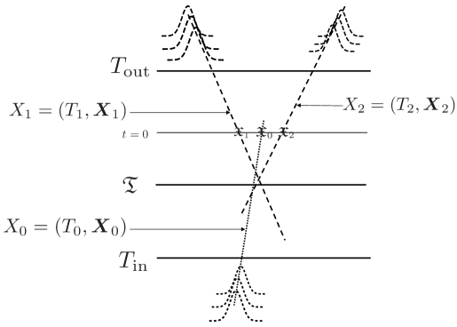
Figure 1: Schematic figure for a configuration with fixed $\Pi_{A}=\left(\boldsymbol{P}_{A},X_{A}\right)$ with $A=0,1,2$. ($\sigma_{A}$ are kept fixed throughout this paper.) Each wave packet is defined at time $T_{A}$ as a free Gaussian wave packet centered at $\boldsymbol{X}_{A}$. Within our leading saddle-point approximation, the widths of the wave packets do not change in time, see Eq. (18), and therefore it does not really matter at which time each wave packet is set to be the free Gaussian wave packet. The wave packets intersect at the time $\mathfrak{T}$, around which the interactions occur most. $\boldsymbol{\mathfrak{X}}_{A}$ is the location of the center of each wave packet at the (arbitrarily chosen) reference time $t=0$. At time $t$, the location of the center moves to $\boldsymbol{\Xi}_{A}\!\left(t\right)=\boldsymbol{\mathfrak{X}}_{A}+\boldsymbol{V}_{A}t$.

Now we compute the Gaussian $S$-matrix. In Sec. 3.1, we obtain the $S$-matrix in the leading saddle-point approximation (18) for the large widths expansion. In Sec. 3.2, we exactly integrate over the spacetime position $x$ of the interaction point. In Sec. 3.3, we separate the bulk and boundary effects. In Sec. 3.4, a limit of large argument is taken to get some physical insight. A schematic figure for this section is presented in Fig. 1.

3.1 Saddle-point approximation in plane-wave limit

With the leading saddle-point approximation (18) in the large width expansion for all the in and out wave packets, we obtain the $S$-matrix for a given configuration $\left(\Pi_{0},\Pi_{1},\Pi_{2}\right)$:

$$S \to{i\kappa\over\sqrt{2}}\left(\prod_{A=0}^{2}\left(\pi\sigma_{A}\right)^{-3/4}{1\over\sqrt{2E_{A}}}\right)e^{-{\sigma_{t}\over 2}\left(\delta\omega\right)^{2}-{\sigma_{s}\over 2}\left(\delta\boldsymbol{P}\right)^{2}-{\mathcal{R}\over 2}+i\left[\cdots\right]}$$

$$\quad\times\int_{T_{\text{in}}}^{T_{\text{out}}}\text{d}t\,e^{-{1\over 2\sigma_{t}}\left[t-\left(\mathfrak{T}+i\sigma_{t}\delta\omega\right)\right]^{2}}\int\text{d}^{3}\boldsymbol{x}\,e^{-{1\over 2\sigma_{s}}\left[\boldsymbol{x}-\left(\overline{\boldsymbol{\mathfrak{X}}}+\overline{\boldsymbol{V}}t-i\sigma_{s}\delta\boldsymbol{P}\right)\right]^{2}},$$ (27)

where the symbols indicate the following:

• $E_{A}$ are the on-shell energies:

  $$E_{A} :=\sqrt{m_{A}^{2}+\boldsymbol{P}_{A}^{2}} (A =0,1,2),$$ (28)

  with $m_{0}:=m_{\Phi}$ and $m_{a}:=m_{\phi}$ ($a=1,2$) being their masses. (This is mere a rephrasing of Eq. (3).)

• $\boldsymbol{V}_{A}$ are the corresponding group velocities:

  $$\boldsymbol{V}_{A} :={\boldsymbol{P}_{A}\over E_{A}}.$$ (29)

  We may freely choose either variable $\boldsymbol{P}_{A}$ or $\boldsymbol{V}_{A}$, which are in one-to-one correspondence.

• $\sqrt{\sigma_{s}}$ is the spatial size of the interaction region:

  $$\sigma_{s} :=\left(\sum_{A=0}^{2}{1\over\sigma_{A}}\right)^{-1}.$$ (30)

  Hereafter, we abbreviate e.g. $\sum_{A=0}^{2}$ to $\sum_{A}$. (We also let the lower-case letters $a,b,\dots$ run for the final states 1 and 2 such that $\sum_{a}:=\sum_{a=1}^{2}$, etc.)

• The overline denotes the following weighted sum (and not the complex conjugate): For arbitrary scalar and three-vector quantities $C_{A}$ and $\boldsymbol{Q}_{A}$, respectively, we define

  $$\overline{C} :=\sigma_{s}\sum_{A}{C_{A}\over\sigma_{A}}, \overline{\boldsymbol{Q}} :=\sigma_{s}\sum_{A}{\boldsymbol{Q}_{A}\over\sigma_{A}}.$$ (31)

  We further define, for any $\boldsymbol{Q}_{A}$,

  $$\Delta\boldsymbol{Q}^{2} :=\overline{\boldsymbol{Q}^{2}}-\overline{\boldsymbol{Q}}^{2},$$ (32)

  where $\overline{\boldsymbol{Q}^{2}}=\sigma_{s}\sum_{A}{\boldsymbol{Q}_{A}^{2}\over\sigma_{A}}$ and $\overline{\boldsymbol{Q}}^{2}=\overline{\boldsymbol{Q}}\cdot\overline{\boldsymbol{Q}}=\sigma_{s}^{2}\sum_{AB}{\boldsymbol{Q}_{A}\cdot\boldsymbol{Q}_{B}\over\sigma_{A}\sigma_{B}}$, which follow from the definition (31).

• $\sqrt{\sigma_{t}}$ is the time-like size of the interaction region:

  $$\sigma_{t} :={\sigma_{s}\over\Delta\boldsymbol{V}^{2}}.$$ (33)

• $\mathfrak{T}$ is what we call the intersection time, around which the interaction occurs:

  $$\mathfrak{T} :=\sigma_{t}{\overline{\boldsymbol{V}}\cdot\overline{\boldsymbol{\mathfrak{X}}}-\overline{\boldsymbol{V}\cdot\boldsymbol{\mathfrak{X}}}\over\sigma_{s}}={\overline{\boldsymbol{V}}\cdot\overline{\boldsymbol{\mathfrak{X}}}-\overline{\boldsymbol{V}\cdot\boldsymbol{\mathfrak{X}}}\over\Delta\boldsymbol{V}^{2}},$$ (34)

  where $\boldsymbol{\mathfrak{X}}_{A}=\boldsymbol{\Xi}_{A}\!\left(0\right)$ is the location of the center of each wave packet at our reference time $t=0$:

  $$\boldsymbol{\mathfrak{X}}_{A}:=\boldsymbol{X}_{A}-\boldsymbol{V}_{A}T_{A}.$$ (35)

• $\mathcal{R}$ is what we will call the overlap exponent that gives the suppression factor accounting for the non-overlap of the wave packets at the intersection point:

  $$\mathcal{R} :={\Delta\boldsymbol{\mathfrak{X}}^{2}\over\sigma_{s}}-{\mathfrak{T}^{2}\over\sigma_{t}}.$$ (36)

• We define the mometum and energy shifts, etc:

  $$\delta\boldsymbol{P} :=\boldsymbol{P}_{1}+\boldsymbol{P}_{2}-\boldsymbol{P}_{0}, \delta E :=E_{1}+E_{2}-E_{0}, \delta\omega :=\delta E-\overline{\boldsymbol{V}}\cdot\delta\boldsymbol{P}.$$ (37)

• “$i\left[\cdots\right]$” denotes the irrelevant pure imaginary terms that are independent of $x$. We will neglect them hereafter as they disappear when we take the absolute square of $S$.

Note that each quantity defined in the above list is a fixed real number for a given configuration of the wave packets $\left(\Pi_{0},\Pi_{1},\Pi_{2}\right)$. Later we will treat $\boldsymbol{X}_{a}$ ($a=1,2$) as variables of six degrees of freedom; others $\mathfrak{T}$, $\boldsymbol{\mathfrak{X}}_{a}$, and $\mathcal{R}$ are dependent ones. (If we vary the final state momenta, then $\boldsymbol{P}_{a}$ ($a=1,2$) also become variables; others $\boldsymbol{V}_{a}$, $\sigma_{t}$, $\delta\boldsymbol{P}$, $\delta E$, and $\delta\omega$ become dependent ones accordingly.)

For any pair of three-vectors $\boldsymbol{Q}_{A}$ and $\boldsymbol{Q}_{A}^{\prime}$ ($A=0,1,2$), we get

$$\overline{\boldsymbol{Q}\cdot\boldsymbol{Q}^{\prime}}-\overline{\boldsymbol{Q}}\cdot\overline{\boldsymbol{Q}^{\prime}} =\sigma_{s}^{2}\left[{\delta\boldsymbol{Q}_{1}\cdot\delta\boldsymbol{Q}_{1}^{\prime}\over\sigma_{0}\sigma_{1}}+{\delta\boldsymbol{Q}_{2}\cdot\delta\boldsymbol{Q}_{2}^{\prime}\over\sigma_{0}\sigma_{2}}+{\left(\delta\boldsymbol{Q}_{1}-\delta\boldsymbol{Q}_{2}\right)\cdot\left(\delta\boldsymbol{Q}_{1}^{\prime}-\delta\boldsymbol{Q}_{2}^{\prime}\right)\over\sigma_{1}\sigma_{2}}\right],$$ (38)

where we define, for any $\boldsymbol{Q}_{A}$,

$$\delta\boldsymbol{Q}_{a} :=\boldsymbol{Q}_{a}-\boldsymbol{Q}_{0}.$$ (39)

Note that we always have $\delta\boldsymbol{Q}_{1}-\delta\boldsymbol{Q}_{2}=\boldsymbol{Q}_{1}-\boldsymbol{Q}_{2}$. Especially,

$$\Delta\boldsymbol{Q}^{2} =\sigma_{s}^{2}\left[{\left(\delta\boldsymbol{Q}_{1}\right)^{2}\over\sigma_{0}\sigma_{1}}+{\left(\delta\boldsymbol{Q}_{2}\right)^{2}\over\sigma_{0}\sigma_{2}}+{\left(\delta\boldsymbol{Q}_{1}-\delta\boldsymbol{Q}_{2}\right)^{2}\over\sigma_{1}\sigma_{2}}\right]$$

$$=\sigma_{s}^{2}\left[{\left(\boldsymbol{Q}_{1}-\boldsymbol{Q}_{0}\right)^{2}\over\sigma_{0}\sigma_{1}}+{\left(\boldsymbol{Q}_{2}-\boldsymbol{Q}_{0}\right)^{2}\over\sigma_{0}\sigma_{2}}+{\left(\boldsymbol{Q}_{1}-\boldsymbol{Q}_{2}\right)^{2}\over\sigma_{1}\sigma_{2}}\right],$$ (40)

or more concretely,

$$\Delta\boldsymbol{\mathfrak{X}}^{2} =\sigma_{s}^{2}\left[{\left(\delta\boldsymbol{\mathfrak{X}}_{1}\right)^{2}\over\sigma_{0}\sigma_{1}}+{\left(\delta\boldsymbol{\mathfrak{X}}_{2}\right)^{2}\over\sigma_{0}\sigma_{2}}+{\left(\delta\boldsymbol{\mathfrak{X}}_{1}-\delta\boldsymbol{\mathfrak{X}}_{2}\right)^{2}\over\sigma_{1}\sigma_{2}}\right],$$ (41)

$$\Delta\boldsymbol{V}^{2} =\sigma_{s}^{2}\left[{\left(\delta\boldsymbol{V}_{1}\right)^{2}\over\sigma_{0}\sigma_{1}}+{\left(\delta\boldsymbol{V}_{2}\right)^{2}\over\sigma_{0}\sigma_{2}}+{\left(\delta\boldsymbol{V}_{1}-\delta\boldsymbol{V}_{2}\right)^{2}\over\sigma_{1}\sigma_{2}}\right].$$ (42)

Then we get

$$\sigma_{t} ={1\over\sigma_{s}}\left[{\left(\delta\boldsymbol{V}_{1}\right)^{2}\over\sigma_{0}\sigma_{1}}+{\left(\delta\boldsymbol{V}_{2}\right)^{2}\over\sigma_{0}\sigma_{2}}+{\left(\delta\boldsymbol{V}_{1}-\delta\boldsymbol{V}_{2}\right)^{2}\over\sigma_{1}\sigma_{2}}\right]^{-1},$$ (43)

$$\mathfrak{T} =-\sigma_{s}\sigma_{t}\left[{\delta\boldsymbol{\mathfrak{X}}_{1}\cdot\delta\boldsymbol{V}_{1}\over\sigma_{0}\sigma_{1}}+{\delta\boldsymbol{\mathfrak{X}}_{2}\cdot\delta\boldsymbol{V}_{2}\over\sigma_{0}\sigma_{2}}+{\left(\delta\boldsymbol{\mathfrak{X}}_{1}-\delta\boldsymbol{\mathfrak{X}}_{2}\right)\cdot\left(\delta\boldsymbol{V}_{1}-\delta\boldsymbol{V}_{2}\right)\over\sigma_{1}\sigma_{2}}\right],$$ (44)

$$\mathcal{R} =\sigma_{s}\Bigg{\{}{\left(\delta\boldsymbol{\mathfrak{X}}_{1}\right)^{2}\over\sigma_{0}\sigma_{1}}+{\left(\delta\boldsymbol{\mathfrak{X}}_{2}\right)^{2}\over\sigma_{0}\sigma_{2}}+{\left(\delta\boldsymbol{\mathfrak{X}}_{1}-\delta\boldsymbol{\mathfrak{X}}_{2}\right)^{2}\over\sigma_{1}\sigma_{2}}$$

$$\qquad-{\sigma_{s}\sigma_{t}}\left[{\delta\boldsymbol{\mathfrak{X}}_{1}\cdot\delta\boldsymbol{V}_{1}\over\sigma_{0}\sigma_{1}}+{\delta\boldsymbol{\mathfrak{X}}_{2}\cdot\delta\boldsymbol{V}_{2}\over\sigma_{0}\sigma_{2}}+{\left(\delta\boldsymbol{\mathfrak{X}}_{1}-\delta\boldsymbol{\mathfrak{X}}_{2}\right)\cdot\left(\delta\boldsymbol{V}_{1}-\delta\boldsymbol{V}_{2}\right)\over\sigma_{1}\sigma_{2}}\right]^{2}\Bigg{\}}.$$ (45)

Note that for a parent particle at rest, $\boldsymbol{P}_{0}=0$, we may simply replace $\delta\boldsymbol{V}_{a}\to\boldsymbol{V}_{a}$. Expressions in various limits are shown in Appendix C.

Let us prove the non-negativity of $\mathcal{R}$. In general, the weighted average for any real vector $\boldsymbol{Q}$ satisfies

$$\Delta\boldsymbol{Q}^{2}=\overline{\boldsymbol{Q}^{2}}-\overline{\boldsymbol{Q}}^{2}=\overline{\left(\boldsymbol{Q}-\overline{\boldsymbol{Q}}\right)^{2}} \geq 0.$$ (46)

From this, one can deduce the non-negativity of $\mathcal{R}$ as follows: At time $t$, the center of each wave packet is located at

$$\boldsymbol{Z}_{A} :=\boldsymbol{\mathfrak{X}}_{A}+\boldsymbol{V}_{A}t.$$ (47)

The square completion of $\Delta\boldsymbol{Z}^{2}=\overline{\boldsymbol{Z}^{2}}-\overline{\boldsymbol{Z}}^{2}$ with respect to $t$ shows that $\Delta\boldsymbol{Z}^{2}$ takes its minimum value $\sigma_{s}\mathcal{R}$ at $t=\mathfrak{T}$:

$$\Delta\boldsymbol{Z}^{2} =\Delta\boldsymbol{V}^{2}\left(t-\mathfrak{T}\right)^{2}+\sigma_{s}\mathcal{R}.$$ (48)

As $\Delta\boldsymbol{Z}^{2}\geq 0$ for any $t$, we obtain $\sigma_{s}\mathcal{R}\geq 0$, hence the non-negativity of $\mathcal{R}$.

In particular, if the center of all the three wave packets coincide at $\boldsymbol{Z}_{A}=\boldsymbol{x}$ at some time $t$, then $\overline{\boldsymbol{Z}}=\boldsymbol{x}$ and $\Delta\boldsymbol{Z}^{2}=0$. Eq. (48) shows that this can be the case when and only when $t=\mathfrak{T}$ (for $\Delta\boldsymbol{V}^{2}>0$) and that we get no suppression in such a case, $\mathcal{R}=0$.

Let us see the physical meaning of $\mathfrak{T}$. Suppose that we recklessly take the particle limit $\sigma_{t},\sigma_{s}\to 0$ in the second line in Eq. (27) even though the expression itself is obtained in the contrary plane-wave expansion. Then we see that the interaction indeed occurs around the spacetime point

$$x=\left(t,\boldsymbol{x}\right)\sim\left(\mathfrak{T},\overline{\boldsymbol{\mathfrak{X}}}+\overline{\boldsymbol{V}}\mathfrak{T}\right),$$ (49)

which we call the intersection point.

One can show (without taking the particle limit) that the intersection point (49) is transformed properly by the spacetime translation: By a constant spacetime translation

$$\boldsymbol{X}_{A} \to\boldsymbol{X}_{A}+\boldsymbol{d},$$

$$T_{A} \to T_{A}+d^{0},$$ (50)

the center of each wave packet (at $t=0$) and its average transform as

$$\boldsymbol{\mathfrak{X}}_{A} \to\boldsymbol{\mathfrak{X}}_{A}+\boldsymbol{d}-\boldsymbol{V}_{A}d^{0},$$ (51)

$$\overline{\boldsymbol{\mathfrak{X}}} \to\overline{\boldsymbol{\mathfrak{X}}}+\boldsymbol{d}-\overline{\boldsymbol{V}}d^{0},$$ (52)

and hence

$$\mathfrak{T} \to\mathfrak{T}+d^{0},$$ (53)

$$\left(\overline{\boldsymbol{\mathfrak{X}}}+\overline{V}\mathfrak{T}\right) \to\left(\overline{\boldsymbol{\mathfrak{X}}}+\overline{V}\mathfrak{T}\right)+\boldsymbol{d}.$$ (54)

One can also check that the overlap exponent $\mathcal{R}$ is translationally invariant (as it should physically be):

$$\mathcal{R} \to\mathcal{R}.$$ (55)

In particular, we may choose

$$\boldsymbol{d}=\boldsymbol{V}_{0}d^{0},$$ (56)

such that the center of the initial wave packet at $t=0$, $\boldsymbol{\mathfrak{X}}_{0}=\boldsymbol{X}_{0}-\boldsymbol{V}_{0}T_{0}$, is kept invariant. Then the center of each final-state wave packet, $\boldsymbol{\mathfrak{X}}_{a}$, is shifted as

$$\boldsymbol{\mathfrak{X}}_{a} \to\boldsymbol{\mathfrak{X}}_{a}-\delta\boldsymbol{V}_{a}d^{0}, \delta\boldsymbol{\mathfrak{X}}_{a} \to\delta\boldsymbol{\mathfrak{X}}_{a}-\delta\boldsymbol{V}_{a}d^{0}.$$ (57)

Later, this translation will correspond to the zero mode (91).

3.2 Spacetime integral over position of interaction point

One can exactly perform the Gaussian integrals over the interaction point $x=\left(t,\boldsymbol{x}\right)$ in Eq. (27) to get

$$S ={i\kappa\over\sqrt{2}}\left(\prod_{A}\left(\pi\sigma_{A}\right)^{-3/4}{1\over\sqrt{2E_{A}}}\right)e^{-{\sigma_{t}\over 2}\left(\delta\omega\right)^{2}-{\sigma_{s}\over 2}\left(\delta\boldsymbol{P}\right)^{2}-{\mathcal{R}\over 2}}\left(2\pi\sigma_{s}\right)^{3/2}\sqrt{2\pi\sigma_{t}}\,G\!\left(\mathfrak{T}\right),$$ (58)

where we have defined the window function:

$$G\!\left(\mathfrak{T}\right) :=\int_{T_{\text{in}}}^{T_{\text{out}}}{\text{d}t\over\sqrt{2\pi\sigma_{t}}}e^{-{1\over 2\sigma_{t}}\left(t-\mathfrak{T}-i\sigma_{t}\delta\omega\right)^{2}}$$

$$={1\over 2}\left[\operatorname{erf}\!\left(\mathfrak{T}-T_{\text{in}}+i\sigma_{t}\delta\omega\over\sqrt{2\sigma_{t}}\right)-\operatorname{erf}\!\left(\mathfrak{T}-T_{\text{out}}+i\sigma_{t}\delta\omega\over\sqrt{2\sigma_{t}}\right)\right],$$ (59)

in which

$$\operatorname{erf}\!\left(z\right) :={2\over\sqrt{\pi}}\int_{0}^{z}e^{-x^{2}}\text{d}x$$ (60)

is the Gauss error function. In the small and large $\left|z\right|$ limits, its (asymptotic) expansion reads, respectively,

$$\operatorname{erf}\!\left(z\right) ={2z\over\sqrt{\pi}}+\mathcal{O}\!\left(z^{3}\right),$$ (61)

$$\operatorname{erf}\!\left(z\right) =\operatorname{sgn}\!\left(z\right)+e^{-z^{2}}\left(-{1\over\sqrt{\pi}z}+\mathcal{O}\!\left(z^{-3}\right)\right),$$ (62)

where we have defined a sign function for a complex variable:

$$\operatorname{sgn}\!\left(z\right) :=\begin{cases}1&\text{for $\Re z>0$ or ($\Re z=0$ and $\Im z>0$),}\\ -1&\text{for $\Re z<0$ or ($\Re z=0$ and $\Im z<0$),}\\ 0&\text{for $z=0$.}\end{cases}$$ (63)

From Eq. (58), we see that the $S$-matrix is exponentially suppressed unless the momentum is nearly conserved, $\delta\boldsymbol{P}\sim 0$. This is also the case for the energy conservation $\delta\omega\sim 0$ except in the boundary regions, at which the translational invariance is explicitly broken; see Sec. 3.4 below. As said above, the overlap exponent $\mathcal{R}$ gives another suppression when the wave packets do not overlap.

3.3 Separation of bulk and boundary effects

It is convenient to separate the window function (59) into the bulk part and the in- and out-boundary ones:

$$G\!\left(\mathfrak{T}\right) =G_{\text{bulk}}\!\left(\mathfrak{T}\right)+G_{\text{in-bdry}}\!\left(\mathfrak{T}\right)+G_{\text{out-bdry}}\!\left(\mathfrak{T}\right),$$ (64)

where

$$G_{\text{bulk}}\!\left(\mathfrak{T}\right) :={1\over 2}\left[\operatorname{sgn}\!\left(\mathfrak{T}-T_{\text{in}}+i\sigma_{t}\delta\omega\over\sqrt{2\sigma_{t}}\right)-\operatorname{sgn}\!\left(\mathfrak{T}-T_{\text{out}}+i\sigma_{t}\delta\omega\over\sqrt{2\sigma_{t}}\right)\right],$$ (65)

$$G_{\text{in-bdry}}\!\left(\mathfrak{T}\right) :={1\over 2}\left[\operatorname{erf}\!\left(\mathfrak{T}-T_{\text{in}}+i\sigma_{t}\delta\omega\over\sqrt{2\sigma_{t}}\right)-\operatorname{sgn}\!\left(\mathfrak{T}-T_{\text{in}}+i\sigma_{t}\delta\omega\over\sqrt{2\sigma_{t}}\right)\right],$$

$$G_{\text{out-bdry}}\!\left(\mathfrak{T}\right) :={1\over 2}\left[\operatorname{sgn}\!\left(\mathfrak{T}-T_{\text{out}}+i\sigma_{t}\delta\omega\over\sqrt{2\sigma_{t}}\right)-\operatorname{erf}\!\left(\mathfrak{T}-T_{\text{out}}+i\sigma_{t}\delta\omega\over\sqrt{2\sigma_{t}}\right)\right].$$ (66)

One can rewrite the boundary parts:

$$G_{\text{in-bdry}}\!\left(\mathfrak{T}\right) ={1\over 2}G_{\text{bdry}}\!\left(\mathfrak{T}-T_{\text{in}}+i\sigma_{t}\delta\omega\over\sqrt{2\sigma_{t}}\right),$$ (67)

$$G_{\text{out-bdry}}\!\left(\mathfrak{T}\right) =-{1\over 2}G_{\text{bdry}}\!\left(\mathfrak{T}-T_{\text{out}}+i\sigma_{t}\delta\omega\over\sqrt{2\sigma_{t}}\right),$$ (68)

where

$$G_{\text{bdry}}\!\left(z\right) :=\operatorname{erf}\!\left(z\right)-\operatorname{sgn}\!\left(z\right).$$ (69)

More explicitly, the bulk part reads

$$G_{\text{bulk}}\!\left(\mathfrak{T}\right) =\begin{cases}1&(T_{\text{in}}<\mathfrak{T}<T_{\text{out}}),\\ 0&(\mathfrak{T}<T_{\text{in}}\text{ or }T_{\text{out}}<\mathfrak{T}),\\ \theta\!\left(\delta\omega\right)&(\mathfrak{T}=T_{\text{in}}),\\ \theta\!\left(-\delta\omega\right)&(\mathfrak{T}=T_{\text{out}}),\end{cases}$$ (70)

where

$$\theta\!\left(x\right) ={1+\operatorname{sgn}\!\left(x\right)\over 2}=\begin{cases}1&(x>0),\\ {1\over 2}&(x=0),\\ 0&(x<0),\end{cases}$$ (71)

is the step function.

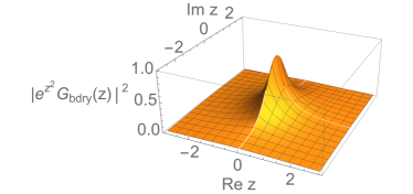
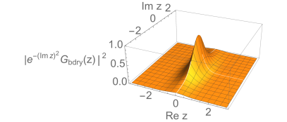
Figure 2: Normalized boundary function $\left|e^{z^{2}}G_{\text{bdry}}\!\left(z\right)\right|^{2}$ (left) and the combination that appears in physical setup $\left|e^{-\left(\Im z\right)^{2}}G_{\text{bdry}}\!\left(z\right)\right|^{2}$ (right).

We note that $G_{\text{bdry}}\!\left(z\right)$ is discontinuous at $\Re z=0$ but the combination $\left|e^{z^{2}}G_{\text{bdry}}\!\left(z\right)\right|^{2}$ is continuous and finite everywhere on the complex $z$ plane (except at the origin $z=0$); see Fig. 2. Especially in the limit $\left|z\right|\to\infty$, we obtain

$$\left|e^{z^{2}}G_{\text{bdry}}\!\left(z\right)\right|^{2} \to{1\over\pi\left|z\right|^{2}}.$$ (72)

The explicit formula in the boundary limit $\left|\mathfrak{T}-T_{\text{in/out}}\right|\ll\sigma_{t}\delta\omega$ is

$$G_{\text{bdry}}\!\left(\mathfrak{T}-T_{\text{in/out}}+i\sigma_{t}\delta\omega\over\sqrt{2\sigma_{t}}\right) \to\pm{2i\over\sqrt{\pi}}F\!\left(\sqrt{\sigma_{t}\over 2}\delta\omega\right)e^{{\sigma_{t}\over 2}\left(\delta\omega\right)^{2}}\mp\begin{cases}\operatorname{sgn}\!\left(\delta\omega\right)&\text{for }\mathfrak{T}=T_{\text{in/out}},\\ \operatorname{sgn}\!\left(\mathfrak{T}-T_{\text{in/out}}\right)&\text{for }\mathfrak{T}\neq T_{\text{in/out}},\end{cases}$$ (73)

that is,

$$e^{-\sigma_{t}\left(\delta\omega\right)^{2}}\left|G_{\text{bdry}}\!\left(\mathfrak{T}-T_{\text{in/out}}+i\sigma_{t}\delta\omega\over\sqrt{2\sigma_{t}}\right)\right|^{2} \to{4\over\pi}F^{2}\!\left(\sqrt{\sigma_{t}\over 2}\delta\omega\right)+e^{-\sigma_{t}\left(\delta\omega\right)^{2}},$$ (74)

where

$$F\!\left(x\right) :=e^{-x^{2}}\int_{0}^{x}e^{z^{2}}\text{d}z=-i{\sqrt{\pi}\over 2}e^{-x^{2}}\operatorname{erf}\!\left(ix\right)$$ (75)

is the Dawson function, whose (asymptotic) expansions read

$$F\!\left(x\right) =x+\mathcal{O}\!\left(x^{3}\right),$$ (76)

$$F\!\left(x\right) =-i{\sqrt{\pi}\over 2}e^{-x^{2}}\operatorname{sgn}\!\left(ix\right)+{1\over 2x}+\mathcal{O}\!\left(1\over x^{3}\right).$$ (77)

More explicitly, the large $\sqrt{\sigma_{t}}\delta\omega$ expansion gives

$${4\over\pi}F^{2}\!\left(\sqrt{\sigma_{t}\over 2}\delta\omega\right)+e^{-\sigma_{t}\left(\delta\omega\right)^{2}} ={2\over\pi}{1\over\sigma_{t}\left(\delta\omega\right)^{2}}+\mathcal{O}\!\left({1\over\sigma_{t}^{2}\left(\delta\omega\right)^{4}}\right).$$ (78)

In Fig. 3, we plot $G_{\text{bdry}}$ right at either boundary $\mathfrak{T}=T_{\text{in/out}}$.

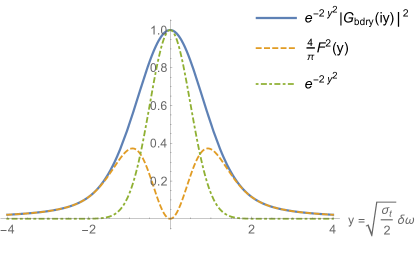
Figure 3: We plot $e^{-2y^{2}}\left|G_{\text{bdry}}\!\left(iy\right)\right|^{2}$ (solid), ${4\over\pi}F^{2}\!\left(y\right)$ (dashed), and $e^{-2y^{2}}$ (dot-dashed) as a function of $y=\sqrt{\sigma_{t}\over 2}\delta\omega$, which corresponds to right on either boundary $\mathfrak{T}=T_{\text{in/out}}$. The solid line is the sum of the dashed and dot-dashed lines and corresponds to the ridge line at $\Re z=0$ in Fig. 2.

3.4 Limit of large argument

In the limit

$${\left|\mathfrak{T}-T_{\text{in}}+i\sigma_{t}\delta\omega\right|\over\sqrt{\sigma_{t}}},{\left|\mathfrak{T}-T_{\text{out}}+i\sigma_{t}\delta\omega\right|\over\sqrt{\sigma_{t}}}\gg 1,$$ (79)

the possible leading contributions are

$$G\!\left(\mathfrak{T}\right) \to{1\over 2}\bigg{[}\operatorname{sgn}\!\left(\mathfrak{T}-T_{\text{in}}+i\sigma_{t}\delta\omega\over\sqrt{2\sigma_{t}}\right)-\operatorname{sgn}\!\left(\mathfrak{T}-T_{\text{out}}+i\sigma_{t}\delta\omega\over\sqrt{2\sigma_{t}}\right)$$

$$\phantom{\to{1\over 2}\bigg{[}}-e^{-{\left(\mathfrak{T}-T_{\text{in}}\right)^{2}\over 2\sigma_{t}}+{\sigma_{t}\over 2}\left(\delta\omega\right)^{2}-i\,\delta\omega\left(\mathfrak{T}-T_{\text{in}}\right)}\sqrt{2\sigma_{t}\over\pi}{1\over\mathfrak{T}-T_{\text{in}}+i\sigma_{t}\delta\omega}$$

$$\phantom{\to{1\over 2}\bigg{[}}+e^{-{\left(\mathfrak{T}-T_{\text{out}}\right)^{2}\over 2\sigma_{t}}+{\sigma_{t}\over 2}\left(\delta\omega\right)^{2}-i\,\delta\omega\left(\mathfrak{T}-T_{\text{out}}\right)}\sqrt{2\sigma_{t}\over\pi}{1\over\mathfrak{T}-T_{\text{out}}+i\sigma_{t}\delta\omega}\bigg{]}.$$ (80)

We see that the range of $\mathfrak{T}$ in this limit can be separated into the following regions:

• In the bulk region

  $$\left|\mathfrak{T}-T_{\text{in}}\right|,\left|\mathfrak{T}-T_{\text{out}}\right|\gg\sigma_{t}\delta\omega,$$ (81)

  where the intersection time $\mathfrak{T}$ is well separated from both the boundary times $T_{\text{in}}$ and $T_{\text{out}}$, we obtain

  $$G\!\left(\mathfrak{T}\right) \to W\!\left(\mathfrak{T}\right):=\begin{cases}1&(T_{\text{in}}<\mathfrak{T}<T_{\text{out}}),\\ 0&\text{(otherwise),}\end{cases}$$ (82)

  hence the name “window function.”

• In the in and out boundary regions $\mathfrak{T}\sim T_{\text{in}}$ and $T_{\text{out}}$ (namely $\left|\mathfrak{T}-T_{\text{in}}\right|\lesssim\sigma_{t}\delta\omega$ and $\left|\mathfrak{T}-T_{\text{out}}\right|\lesssim\sigma_{t}\delta\omega$), the contribution from the second and third lines, respectively, in Eq. (80) becomes sizable:

  $$e^{-\sigma_{t}\left(\delta\omega\right)^{2}}\left|G\!\left(\mathfrak{T}\right)\right|^{2} \to e^{-{\left(\mathfrak{T}-T_{\text{in/out}}\right)^{2}\over\sigma_{t}}}{2\over\pi}{1\over{\left(\mathfrak{T}-T_{\text{in/out}}\right)^{2}\over\sigma_{t}}+\sigma_{t}\left(\delta\omega\right)^{2}}.$$ (83)

  We see that the exponential suppression $e^{-\sigma_{t}\left(\delta\omega\right)^{2}}$ for $\sigma_{t}\left(\delta\omega\right)^{2}\gg 1$ becomes absent in the boundary region.

In Refs. [8, 9, 11, 10], the authors have claimed that contributions from the boundary region can become non-negligible and that there can be physical consequences. In this paper, we leave this issue open and proceed by taking into account only the bulk region contribution (82); we will briefly comment on the boundary effects in Sec. 4.3.

Eq. (83) appears singular in the simultaneous limit $\left|\mathfrak{T}-T_{\text{in/out}}\right|\to 0$ and $\sigma_{t}\delta\omega\to 0$. This apparent singularity is an artifact of first taking the limit (80): If we take the limit $\left|\mathfrak{T}-T_{\text{in/out}}+i\sigma_{t}\delta\omega\right|\ll\sqrt{\sigma_{t}}$ in the original expression (59), we obtain

$$e^{-\sigma_{t}\left(\delta\omega\right)^{2}}\left|G\!\left(\mathfrak{T}\right)\right|^{2} \to{\left(\mathfrak{T}-T_{\text{in/out}}\right)^{2}+\left(\sigma_{t}\delta\omega\right)^{2}\over 2\pi\sigma_{t}}.$$ (84)

It is manifest that we have no singularity.

4 Decay probability: derivation of Fermi’s golden rule

Recalling the (over-)completeness of the Gaussian basis (143), we see that the decay probability into an infinitesimal phase-space range $[\boldsymbol{X}_{a},\boldsymbol{X}_{a}+\text{d}\boldsymbol{X}_{a}]$ and $[\boldsymbol{P}_{a},\boldsymbol{P}_{a}+\text{d}\boldsymbol{P}_{a}]$ ($a=1,2$) is

$$\text{d}P ={\text{d}^{3}\boldsymbol{X}_{1}\,\text{d}^{3}\boldsymbol{P}_{1}\over\left(2\pi\right)^{3}}{\text{d}^{3}\boldsymbol{X}_{2}\,\text{d}^{3}\boldsymbol{P}_{2}\over\left(2\pi\right)^{3}}\left|S\right|^{2}$$

$$={\kappa^{2}\over 2}{1\over 2E_{0}}{\text{d}^{3}\boldsymbol{P}_{1}\over\left(2\pi\right)^{3}2E_{1}}{\text{d}^{3}\boldsymbol{P}_{2}\over\left(2\pi\right)^{3}2E_{2}}\left(2\pi\right)^{4}\left(\sqrt{\sigma_{t}\over\pi}e^{-\sigma_{t}\left(\delta\omega\right)^{2}}\right)\left(\left(\sigma_{s}\over\pi\right)^{3/2}e^{-\sigma_{s}\left(\delta\boldsymbol{P}\right)^{2}}\right)$$

$$\qquad\times\sqrt{{\sigma_{t}\over\pi^{5}}\left(\sigma_{s}\over\sigma_{0}\sigma_{1}\sigma_{2}\right)^{3}}\,\text{d}^{3}\boldsymbol{X}_{1}\,\text{d}^{3}\boldsymbol{X}_{2}\,e^{-\mathcal{R}}\,\left|G\!\left(\mathfrak{T}\right)\right|^{2}.$$ (85)

We note that this expression is exact up to the leading saddle point approximation (18).

In Sec. 4.1, we show how to diagonalize the overlap exponent $\mathcal{R}$. In Sec. 4.2, we focus on the bulk contribution $G_{\text{bulk}}$ and derive the Fermi’s golden rule. In Sec. 4.3, we briefly comment on the boundary contribution $G_{\text{bdry}}$.

4.1 Diagonalization of overlap exponent

Now we want to perform the Gaussian integral over the central positions of the wave packets $\boldsymbol{X}_{a}$. We may rewrite $\mathcal{R}$, in the matrix notation, as follows:

$$\mathcal{R} =\begin{bmatrix}\delta\boldsymbol{\mathfrak{X}}_{1}^{\text{t}}&\delta\boldsymbol{\mathfrak{X}}_{2}^{\text{t}}\end{bmatrix}\mathcal{M}\begin{bmatrix}\delta\boldsymbol{\mathfrak{X}}_{1}\\ \delta\boldsymbol{\mathfrak{X}}_{2}\end{bmatrix},$$ (86)

where the superscript “t” denotes the transposition; as defined in Eq. (39),

$$\delta\boldsymbol{\mathfrak{X}}_{a} :=\boldsymbol{\mathfrak{X}}_{a}-\boldsymbol{\mathfrak{X}}_{0} \delta\boldsymbol{V}_{a} :=\boldsymbol{V}_{a}-\boldsymbol{V}_{0},$$ (87)

for $a=1,2$; and $\mathcal{M}$ is the following real symmetric $6\times 6$ matrix:

$$\mathcal{M} ={\sigma_{s}\over\sigma_{1}\sigma_{2}}\begin{bmatrix}1&-1\\ -1&1\end{bmatrix}+{\sigma_{s}\over\sigma_{0}}\begin{bmatrix}{1\over\sigma_{1}}&0\\ 0&{1\over\sigma_{2}}\end{bmatrix}+\sigma_{s}^{2}\sigma_{t}\begin{bmatrix}\widetilde{\delta\boldsymbol{V}_{1}}\,\widetilde{\delta\boldsymbol{V}_{1}}^{\text{t}}&\widetilde{\delta\boldsymbol{V}_{1}}\,\widetilde{\delta\boldsymbol{V}_{2}}^{\text{t}}\\ \widetilde{\delta\boldsymbol{V}_{2}}\,\widetilde{\delta\boldsymbol{V}_{1}}^{\text{t}}&\widetilde{\delta\boldsymbol{V}_{2}}\,\widetilde{\delta\boldsymbol{V}_{2}}^{\text{t}}\end{bmatrix},$$ (88)

in which

$$\widetilde{\delta\boldsymbol{V}_{1}} :={\delta\boldsymbol{V}_{1}\over\sigma_{0}\sigma_{1}}+{\delta\boldsymbol{V}_{1}-\delta\boldsymbol{V}_{2}\over\sigma_{1}\sigma_{2}}={1\over\sigma_{1}}\left[\left({1\over\sigma_{0}}+{1\over\sigma_{2}}\right)\delta\boldsymbol{V}_{1}-{\delta\boldsymbol{V}_{2}\over\sigma_{2}}\right],$$ (89)

$$\widetilde{\delta\boldsymbol{V}_{2}} :={\delta\boldsymbol{V}_{2}\over\sigma_{0}\sigma_{2}}-{\delta\boldsymbol{V}_{1}-\delta\boldsymbol{V}_{2}\over\sigma_{1}\sigma_{2}}={1\over\sigma_{2}}\left[\left({1\over\sigma_{0}}+{1\over\sigma_{1}}\right)\delta\boldsymbol{V}_{2}-{\delta\boldsymbol{V}_{1}\over\sigma_{1}}\right].$$ (90)

Hereafter, we employ the shifted $\delta\boldsymbol{\mathfrak{X}}_{a}=\boldsymbol{X}_{a}-\left(\boldsymbol{V}_{a}T_{a}+\boldsymbol{X}_{0}-\boldsymbol{V}_{0}T_{0}\right)$ as six integration variables.

One can check that $\mathcal{M}$ has a zero eigenvector:

$$\mathcal{M}\overrightarrow{\mathcal{X}_{0}} =0, \overrightarrow{\mathcal{X}_{0}} ={1\over\sqrt{\left(\delta\boldsymbol{V}_{1}\right)^{2}+\left(\delta\boldsymbol{V}_{2}\right)^{2}}}\begin{bmatrix}\delta\boldsymbol{V}_{1}\\ \delta\boldsymbol{V}_{2}\end{bmatrix},$$ (91)

where we have normalized $\overrightarrow{\mathcal{X}_{0}}$ as $\overrightarrow{\mathcal{X}_{0}}^{\text{t}}\,\overrightarrow{\mathcal{X}_{0}}=1$. This is a direct consequence of the translational invariance under Eq. (57). This zero-mode will eventually give the factor $T_{\text{out}}-T_{\text{in}}$, which is the characteristic of the Fermi’s golden rule.

Writing other five normalized eigenvectors $\overrightarrow{\mathcal{X}_{I}}$ ($I=1,\dots,5$), we get

$$\mathcal{O}^{\text{t}}\mathcal{M}\mathcal{O} =\operatorname{diag}\left(0,\lambda_{1},\dots,\lambda_{5}\right), \mathcal{M} =\sum_{I=1}^{5}\lambda_{I}\overrightarrow{\mathcal{X}_{I}}\overrightarrow{\mathcal{X}_{I}}^{\text{t}},$$ (92)

where $\mathcal{O}:=\begin{bmatrix}\overrightarrow{\mathcal{X}_{0}}&\overrightarrow{\mathcal{X}_{1}}&\cdots&\overrightarrow{\mathcal{X}_{5}}\end{bmatrix}$. Explicit forms of the other five eigenvalues $\lambda_{1},\dots,\lambda_{5}$ are

$${\sigma_{s}\over 2\sigma_{0}}\left({1\over\sigma_{1}}+{1\over\sigma_{2}}\right)+{\sigma_{s}\over\sigma_{1}\sigma_{2}}\left(1\pm\sqrt{1+\left(\sigma_{1}-\sigma_{2}\over 2\sigma_{0}\right)^{2}}\right), {\sigma_{s}\sigma_{t}\over\sigma_{0}\sigma_{1}\sigma_{2}}\left(\left(\delta\boldsymbol{V}_{1}\right)^{2}+\left(\delta\boldsymbol{V}_{2}\right)^{2}\right),$$ (93)

where we have assumed $\Delta\boldsymbol{V}^{2}>0$ in deriving the former, which is two-fold degenerate per each $\pm$ sign, providing four of the five. After some computation, we obtain

$$\prod_{I=1}^{5}\lambda_{I} =\sigma_{t}\left(\sigma_{s}\over\sigma_{0}\sigma_{1}\sigma_{2}\right)^{3}\left(\left(\delta\boldsymbol{V}_{1}\right)^{2}+\left(\delta\boldsymbol{V}_{2}\right)^{2}\right).$$ (94)

We define new integration variables $\left(y_{0},y_{1},\dots,y_{5}\right)$ by

$$\begin{bmatrix}y_{0}\\ \vdots\\ y_{5}\end{bmatrix} =\mathcal{O}^{\text{t}}\begin{bmatrix}\delta\boldsymbol{\mathfrak{X}}_{1}\\ \delta\boldsymbol{\mathfrak{X}}_{2}\end{bmatrix}, \begin{bmatrix}\delta\boldsymbol{\mathfrak{X}}_{1}\\ \delta\boldsymbol{\mathfrak{X}}_{2}\end{bmatrix} =\mathcal{O}\begin{bmatrix}y_{0}\\ \vdots\\ y_{5}\end{bmatrix}.$$ (95)

In particular, we get

$$y_{0} ={\delta\boldsymbol{V}_{1}\cdot\delta\boldsymbol{\mathfrak{X}}_{1}+\delta\boldsymbol{V}_{2}\cdot\delta\boldsymbol{\mathfrak{X}}_{2}\over\sqrt{\left(\delta\boldsymbol{V}_{1}\right)^{2}+\left(\delta\boldsymbol{V}_{2}\right)^{2}}}.$$ (96)

As said above, the integral over $y_{0}$ does not have a Gaussian suppression and will yield the factor $\propto\left(T_{\text{out}}-T_{\text{in}}\right)$. Note that

$$\text{d}^{3}\boldsymbol{X}_{1}\,\text{d}^{3}\boldsymbol{X}_{2}=\text{d}^{6}y$$ (97)

as $\mathcal{O}$ is a special orthogonal matrix.

4.2 Bulk contribution: derivation of Fermi’s golden rule

Now we concentrate on the bulk contribution (65). Physically, this takes into account the bulk region (81), in which the window function takes the particularly simple form (82), by which the spatial $\text{d}^{6}y$ integral is confined within the range that satisfies

$$T_{\text{in}}<\mathfrak{T}<T_{\text{out}},$$ (98)

where the explicit form of $\mathfrak{T}$ is given in Eq. (44). We note that $\mathfrak{T}$ is linear in $\delta\boldsymbol{\mathfrak{X}}_{a}$, and hence in $y_{I}$.

In a typical non-singular configuration of $\left(\boldsymbol{P}_{1},\boldsymbol{P}_{2}\right)$ with $\Delta\boldsymbol{V}^{2}>0$, the integral over all the other five variables $y_{1},\dots,y_{5}$ are confined by the Gaussian factor within the range of the order of $\sqrt{\sigma_{s}}$; see Eq. (93). By definition, the interaction point of the bulk region is well separated from the boundaries, and hence the window function can be regarded as unity for the integral over $y_{1},\dots,y_{5}$. That is, we may safely perform each integral over these five variables as simply Gaussian:

$$\int\text{d}^{5}y\,e^{-\mathcal{R}} =\sqrt{\pi^{5}\over\prod_{I=1}^{5}\lambda_{I}}=\sqrt{{\pi^{5}\over\sigma_{t}}\left(\sigma_{0}\sigma_{1}\sigma_{2}\over\sigma_{s}\right)^{3}}{1\over\sqrt{\left(\delta\boldsymbol{V}_{1}\right)^{2}+\left(\delta\boldsymbol{V}_{2}\right)^{2}}},$$ (99)

in which we used the product of eigenvalues given in Eq. (94).

Rewriting $\delta\boldsymbol{\mathfrak{X}}_{a}$ in Eq. (44) by $y_{0},\dots,y_{5}$ using the latter of Eq. (95), $\begin{bmatrix}\delta\boldsymbol{\mathfrak{X}}_{1}\\ \delta\boldsymbol{\mathfrak{X}}_{2}\end{bmatrix}=\sum_{I=0}^{5}\overrightarrow{\mathcal{X}_{I}}\,y_{I}$, we can read off the coefficient of $y_{0}$ in $\mathfrak{T}$. After some computation, we obtain

$$\mathfrak{T} =-{y_{0}\over\sqrt{\left(\delta\boldsymbol{V}_{1}\right)^{2}+\left(\delta\boldsymbol{V}_{2}\right)^{2}}}+\cdots,$$ (100)

where the dots denote the terms linear in $y_{1},\dots,y_{5}$, which are fixed to be of the order of $\sqrt{\sigma_{s}}$ by the above Gaussian integrals and are neglected hereafter. Now the region of the window function $T_{\text{in}}<\mathfrak{T}<T_{\text{out}}$ corresponds to

$$-\sqrt{\left(\delta\boldsymbol{V}_{1}\right)^{2}+\left(\delta\boldsymbol{V}_{2}\right)^{2}}\,T_{\text{out}}<y_{0}<-\sqrt{\left(\delta\boldsymbol{V}_{1}\right)^{2}+\left(\delta\boldsymbol{V}_{2}\right)^{2}}\,T_{\text{in}},$$ (101)

and the $y_{0}$ integral yields

$$\int\text{d}y_{0}W\!\left(\mathfrak{T}\right) =\sqrt{\left(\delta\boldsymbol{V}_{1}\right)^{2}+\left(\delta\boldsymbol{V}_{2}\right)^{2}}\left(T_{\text{out}}-T_{\text{in}}\right).$$ (102)

To summarize, the integral over $\left(\boldsymbol{X}_{1},\boldsymbol{X}_{2}\right)$ results in

$$\text{d}P ={\kappa^{2}\over 2}{1\over 2E_{0}}{\text{d}^{3}\boldsymbol{P}_{1}\over\left(2\pi\right)^{3}2E_{1}}{\text{d}^{3}\boldsymbol{P}_{2}\over\left(2\pi\right)^{3}2E_{2}}\left(2\pi\right)^{4}\left(\sqrt{\sigma_{t}\over\pi}e^{-\sigma_{t}\left(\delta\omega\right)^{2}}\right)\left(\left(\sigma_{s}\over\pi\right)^{3/2}e^{-\sigma_{s}\left(\delta\boldsymbol{P}\right)^{2}}\right)\left(T_{\text{out}}-T_{\text{in}}\right).$$ (103)

In the wave limit $\sigma_{s},\sigma_{t}\to\infty$, we obtain

$${\text{d}P\over T_{\text{out}}-T_{\text{in}}} ={\kappa^{2}\over 2}{1\over 2E_{0}}\left(\text{d}^{3}\boldsymbol{P}_{1}\over\left(2\pi\right)^{3}2E_{1}\right)\left(\text{d}^{3}\boldsymbol{P}_{2}\over\left(2\pi\right)^{3}2E_{2}\right)\left(2\pi\right)^{4}\delta^{4}\!\left(P_{1}+P_{2}-P_{0}\right).$$ (104)

This is nothing but the Fermi’s golden rule: the decay probability per time-interval $T_{\text{out}}-T_{\text{in}}$. The resultant total decay rate reads

$${P\over T_{\text{out}}-T_{\text{in}}} ={\kappa^{2}\over 32\pi E_{0}}\sqrt{1-{4m_{\phi}^{2}\over m_{\Phi}^{2}}}.$$ (105)

4.3 Comments on boundary contribution

We examine the contributions (66), which come from either in or out boundary region $\left|\mathfrak{T}-T_{\text{in/out}}\right|\lesssim\sigma_{t}\delta\omega$ (tentatively closing our eyes on the point discussed in footnote 19). Formulae for the boundary contributions in the boundary limit are summarized in Appendix (D).

Let us estimate the effect of the $\text{d}^{6}y$ integral over the Gaussian peak $e^{-\left(\mathfrak{T}-T_{\text{in/out}}\right)^{2}/\sigma_{t}}$ in Eq (83), which results from the limit ${\left(\mathfrak{T}-T_{\text{in/out}}\right)^{2}\over\sigma_{t}}+\sigma_{t}\left(\delta\omega\right)^{2}\gg 1$:

$$\text{d}P \to{\kappa^{2}\over 2}{1\over 2E_{0}}{\text{d}^{3}\boldsymbol{P}_{1}\over\left(2\pi\right)^{3}2E_{1}}{\text{d}^{3}\boldsymbol{P}_{2}\over\left(2\pi\right)^{3}2E_{2}}\left(2\pi\right)^{4}\left(\sqrt{\sigma_{t}\over\pi}\right)\left(\left(\sigma_{s}\over\pi\right)^{3/2}e^{-\sigma_{s}\left(\delta\boldsymbol{P}\right)^{2}}\right)$$

$$\qquad\times\sqrt{{\sigma_{t}\over\pi^{5}}\left(\sigma_{s}\over\sigma_{0}\sigma_{1}\sigma_{2}\right)^{3}}\,\text{d}^{6}y\,e^{-\mathcal{R}}e^{-{\left(\mathfrak{T}-T_{\text{in/out}}\right)^{2}\over\sigma_{t}}}{2\over\pi}{1\over{\left(\mathfrak{T}-T_{\text{in/out}}\right)^{2}\over\sigma_{t}}+\sigma_{t}\left(\delta\omega\right)^{2}}.$$ (106)

As discussed in the paragraph containing Eq. (84), this expression is valid only when $\sigma_{t}\left(\delta\omega\right)^{2}\gg 1$ at $\mathfrak{T}=T_{\text{in/out}}$; see Appendix D for possible generalization.

Naively, the integral over the above-mentioned Gaussian peak would be estimated by taking the formal limit $\sigma_{t}\to 0$,

$$e^{-{\left(\mathfrak{T}-T_{\text{in/out}}\right)^{2}\over\sigma_{t}}} \to\sqrt{\pi\sigma_{t}}\,\delta\!\left(\mathfrak{T}-T_{\text{in/out}}\right),$$ (107)

and by regarding the integral $\text{d}^{5}y\,e^{-\mathcal{R}}$ as Gaussian (99); the remaining $y_{0}$ integral would again give the factor $\sqrt{\left(\delta\boldsymbol{V}_{1}\right)^{2}+\left(\delta\boldsymbol{V}_{2}\right)^{2}}$:

$$\text{d}P \sim{\kappa^{2}\over 2}{1\over 2E_{0}}{\text{d}^{3}\boldsymbol{P}_{1}\over\left(2\pi\right)^{3}2E_{1}}{\text{d}^{3}\boldsymbol{P}_{2}\over\left(2\pi\right)^{3}2E_{2}}\left(2\pi\right)^{4}\left[\left(\sigma_{s}\over\pi\right)^{3/2}e^{-\sigma_{s}\left(\delta\boldsymbol{P}\right)^{2}}\right]{2\over\pi}{1\over\left(\delta\omega\right)^{2}}.$$ (108)

We may further take the plane-wave limit $\sigma_{s}\to\infty$, which renders the factor in the square brackets into the delta function $\delta^{3}\!\left(\delta\boldsymbol{P}\right)$:

$$\text{d}P ={\kappa^{2}\over 2}{1\over 2E_{0}}{\text{d}^{3}\boldsymbol{P}_{1}\over\left(2\pi\right)^{3}2E_{1}}{1\over\left(2\pi\right)^{3}2E_{2}}\left(2\pi\right)^{4}{2\over\pi}{1\over\left(\delta E\right)^{2}},$$ (109)

where we have also replaced $\delta\omega$ by $\delta E$; see Eq. (37). We see that the ultraviolet behavior of the momentum integral is

$$\text{d}P \propto\int{\text{d}\left|\boldsymbol{P}_{1}\right|\over\left|\boldsymbol{P}_{1}\right|^{2}},$$ (110)

which is convergent. This convergence itself is independent of the limits that we have taken.

There is no ultraviolet divergence from the boundary regions if the decay is due to the superrenormalizable interaction (1). In contrast, if the decay of scalar were due to a marginal operator of dimension four, we would have got a linearly divergent integral instead of Eq (110).

We comment on the possible ultraviolet divergence at the boundary. First, one might want to take into account the “uncertainty” of $T_{\text{in/out}}$ that is defined in our treatment to be the time (at which the interacting state can well be identified to the free state), by “diffusing the boundary” à la Stueckelberg [12]. This would provide an additional UV suppression factor on the momentum integral, but the necessary unitarity violation requires the change of very definition of the $S$-matrix. Second, as said in footnote 19, the identification of the interacting state with the free state at $T_{\text{in/out}}$ cannot be justified for the boundary contribution. Third, in realistic (particle physics) situation, there is no ideally-sharp time boundary but some production and detection mechanisms that are extended in spacetime. The phenomenology on the boundary region could strongly depend on the microscopic physics of the boundary. Thus, the boundary contribution depends on the situation or might not be valid when it is ultraviolet divergent. Further discussion and implication will be presented elsewhere.

5 Diphoton decay

In order to exhibit how to generalize the simplest scalar decay by the interaction (1) to more realistic cases, we consider the decay of a pseudoscalar into a diphoton pair:

$$\mathcal{L}_{\text{int}} =-{g_{\Phi}\over 4}\Phi\varepsilon_{\lambda\mu\nu\rho}F^{\lambda\mu}F^{\nu\rho}=-\mathcal{H}_{\text{int}},$$ (111)

where $\varepsilon^{\lambda\mu\nu\rho}$ is the totally anti-symmetric tensor and $g_{\Phi}$ is a coupling constant of mass dimension $-1$. For the pion decay, we set $g_{\Phi}={\sqrt{2}\alpha\over\pi f_{\pi}}$, where $\alpha\simeq 1/137$ and $f_{\pi}\simeq 130\,\text{MeV}$ are the fine-structure and pion decay constants, respectively.

It is actually straightforward to generalize the previous analysis to the diphoton decay. The photon field operator can be expanded in terms of the creation/annihilation operators of the plane and Gaussian waves as

$$\hat{A}_{\mu}\!\left(x\right) =\left.\sum_{s}\int{\text{d}^{3}\boldsymbol{p}\over\sqrt{2p^{0}}\left(2\pi\right)^{3/2}}\left[\hat{a}\!\left(s,\boldsymbol{p}\right)\epsilon_{\mu}\!\left(s,\boldsymbol{p}\right)e^{ip\cdot x}+\hat{a}^{\dagger}\!\left(s,\boldsymbol{p}\right)\epsilon^{*}_{\mu}\!\left(s,\boldsymbol{p}\right)e^{-ip\cdot x}\right]\right|_{p^{0}=\left|\boldsymbol{p}\right|}$$ (112)

$$=\sum_{s}\int{\text{d}^{3}\boldsymbol{X}\text{d}^{3}\boldsymbol{P}\over\left(2\pi\right)^{3}}\left[E_{\mu}\!\left(s,\sigma;X,\boldsymbol{P}\right)\hat{A}\!\left(s,\sigma;X,\boldsymbol{P}\right)+E_{\mu}^{*}\!\left(s,\sigma;X,\boldsymbol{P}\right)\hat{A}^{\dagger}\!\left(s,\sigma;X,\boldsymbol{P}\right)\right],$$ (113)

respectively, where

$$E_{\mu}\!\left(s,\sigma;X,\boldsymbol{P}\right) =\left.\int{\text{d}^{3}\boldsymbol{p}\over\sqrt{2p^{0}}}\epsilon_{\mu}\!\left(s,\boldsymbol{p}\right)e^{ip\cdot\left(x-X\right)-{\sigma\over 2}\left(\boldsymbol{p}-\boldsymbol{P}\right)^{2}}\right|_{p^{0}=\left|\boldsymbol{p}\right|};$$ (114)

see Appendix A.3. The saddle-point approximation in the large-width expansion gives

$$E_{\mu}\!\left(s,\sigma;X,\boldsymbol{P}\right) \simeq\left(\sigma\over\pi\right)^{4/3}\left(2\pi\over\sigma\right)^{3/2}\left(1\over\left(2\pi\right)^{3}2\left|\boldsymbol{P}\right|\right)^{1/2}\epsilon_{\mu}\!\left(s,\boldsymbol{P}\right)e^{-i\left|\boldsymbol{P}\right|\left(t-T\right)+i\boldsymbol{P}\cdot\left(\boldsymbol{x}-\boldsymbol{X}\right)-{\left(\boldsymbol{x}-\boldsymbol{\Xi}\!\left(t\right)\right)^{2}\over 2\sigma}};$$ (115)

see Appendix B.

In obtaining the $S$-matrix, all we have to do is to replace $\kappa$ by

$$\kappa \mapsto g_{\Phi}\,\varepsilon_{\lambda\mu\nu\rho}P_{1}^{\lambda}\epsilon^{\mu*}\!\left(s_{1},\boldsymbol{P}_{1}\right)P_{2}^{\nu}\epsilon^{\rho*}\!\left(s_{2},\boldsymbol{P}_{2}\right)$$ (116)

in Eq. (58). The spin-summed decay probability is then, from Eq. (85),

$$\text{d}P ={2g_{\Phi}^{2}\left(P_{1}\cdot P_{2}\right)^{2}\over 2}{1\over 2E_{0}}{\text{d}^{3}\boldsymbol{P}_{1}\over\left(2\pi\right)^{3}2E_{1}}{\text{d}^{3}\boldsymbol{P}_{2}\over\left(2\pi\right)^{3}2E_{2}}\left(2\pi\right)^{4}\left(\sqrt{\sigma_{t}\over\pi}e^{-\sigma_{t}\left(\delta\omega\right)^{2}}\right)\left(\left(\sigma_{s}\over\pi\right)^{3/2}e^{-\sigma_{s}\left(\delta\boldsymbol{P}\right)^{2}}\right)$$

$$\qquad\times\sqrt{{\sigma_{t}\over\pi^{5}}\left(\sigma_{s}\over\sigma_{0}\sigma_{1}\sigma_{2}\right)^{3}}\,\text{d}^{3}\boldsymbol{X}_{1}\,\text{d}^{3}\boldsymbol{X}_{2}\,e^{-\mathcal{R}}\,\left|G\!\left(\mathfrak{T}\right)\right|^{2}.$$ (117)

where we have used

$$\sum_{s_{1},s_{2}}\left|\varepsilon_{\lambda\mu\nu\rho}P_{1}^{\lambda}\epsilon^{\mu}\!\left(s_{1},\boldsymbol{P}_{1}\right)P_{2}^{\nu}\epsilon^{\rho}\!\left(s_{2},\boldsymbol{P}_{2}\right)\right|^{2} =2\left(P_{1}\cdot P_{2}\right)^{2}.$$ (118)

After taking the plane-wave limit, the final expression for the Fermi’s golden rule (104) becomes

$${\text{d}P\over T_{\text{out}}-T_{\text{in}}} ={g_{\Phi}^{2}m_{\Phi}^{4}\over 8E_{0}}\left(\text{d}^{3}\boldsymbol{P}_{1}\over\left(2\pi\right)^{3}2E_{1}\right)\left(\text{d}^{3}\boldsymbol{P}_{2}\over\left(2\pi\right)^{3}2E_{2}\right)\left(2\pi\right)^{4}\delta^{4}\!\left(P_{1}+P_{2}-P_{0}\right),$$ (119)

where we used, under the momentum delta function and the on-shell condition,

$$P_{1}\cdot P_{2} ={\left(P_{1}+P_{2}\right)^{2}\over 2}={P_{0}^{2}\over 2}=-{m_{\Phi}^{2}\over 2}.$$ (120)

The total decay rate is

$${P\over T_{\text{out}}-T_{\text{in}}} ={g_{\Phi}^{2}m_{\Phi}^{4}\over 64\pi E_{0}}.$$ (121)

That is, the replacement in the final expression reads $\kappa^{2}\mapsto g_{\Phi}^{2}m_{\Phi}^{4}/2$ (and of course $m_{\phi}\mapsto 0$).

6 Summary

We have reformulated the Gaussian $S$-matrix within a finite time interval in the Gaussian wave-packet formalism. The normalizable Gaussian basis allows the computation of the decay probability without the momentum-space $\delta^{4}\!\left(0\right)$ singularity that necessarily appears in the one involving the plane-wave basis. We have performed the exact four dimensional integration over the interaction point $x$ for the decay probability. The unitarity is manifestly maintained throughout the whole computation.

We have proposed a separation of the obtained result into the bulk and boundary parts. This separation corresponds to whether the interaction point is near the time boundary or not and hence is rather intuitive and easy to envisage. The Fermi’s golden rule is derived from the bulk contribution. As a byproduct, we have also shown that the ultraviolet divergence in the boundary contribution is absent for the decay of a scalar into a pair of light scalars by the superrenormalizable interaction, though its physical significance is yet to be confirmed. We have generalized our results to the case of diphoton decay and to more general initial and final state particles.

Acknowledgement

We owe Hiromasa Nakatsuka for valuable contributions at the early stages of this work and for reading the manuscript. We are grateful to Osamu Jinnouchi, Arisa Kubota, Terence Sloan, and Risa Ushioda for stimulating discussion. We thank Akio Hosoya, Izumi Ojima, and Masaharu Tanabashi for useful comments. The work of K.I. and K.O. are in part supported by JSPS KAKENHI Grant Nos. 24340043 (K.I.) and 15K05053 (K.O.).

Appendix

Appendix A Gaussian wave packet formalism

We review and spell out our notation for the Gaussian wave-packet basis [3, 8, 11].

A.1 Heisenberg, Schrödinger, and interaction pictures

We may always separate the total Lagrangian density $\mathcal{L}$ into the free part $\mathcal{L}_{\text{free}}$ that contains quadratic terms in fields and the interaction one $\mathcal{L}_{\text{int}}$ that is the rest:

$$\mathcal{L} =\mathcal{L}_{\text{free}}+\mathcal{L}_{\text{int}}.$$ (122)

Correspondingly, we may separate the Hamiltonian (density) $H$ ($\mathcal{H}$) into the free and interaction parts $H_{\text{free}}$ ($\mathcal{H}_{\text{free}}$) and $H_{\text{int}}$ ($\mathcal{H}_{\text{int}}$), respectively:

$$H =H_{\text{free}}+H_{\text{int}}, \mathcal{H} =\mathcal{H}_{\text{free}}+\mathcal{H}_{\text{int}}.$$ (123)

We list the time dependence of the physical state, operator, and eigenbasis in the Heisenberg, Schrödinger, and interaction pictures in the following table:

Picture		State		Operator		Basis
Heisenberg		$\Ket{\Phi}\!{}^{\text{(H)}}\,$	$\hat{O}^{\text{(H)}}\!\left(t\right)$	$=e^{i\hat{H}t}\hat{O}^{\text{(S)}}e^{-i\hat{H}t}$	$\Ket{\Phi,t}\!{}^{\text{(HB)}}\,$	$=e^{i\hat{H}t}\Ket{\Phi}\!{}^{\text{(SB)}}\,$
Schrödinger	$\Ket{\Phi,t}\!{}^{\text{(S)}}\,$	$=e^{-i\hat{H}t}\Ket{\Phi}\!{}^{\text{(H)}}\,$		$\hat{O}^{\text{(S)}}$		$\Ket{\Phi}\!{}^{\text{(SB)}}\,$
Interaction	$\Ket{\Phi,t}\!{}^{\text{(I)}}\,$	$=e^{i\hat{H}_{\text{free}}t}e^{-i\hat{H}t}\Ket{\Phi}\!{}^{\text{(H)}}\,$	$\hat{O}^{\text{(I)}}\!\left(t\right)$	$=e^{i\hat{H}_{\text{free}}t}\hat{O}^{\text{(S)}}e^{-i\hat{H}_{\text{free}}t}$	$\Ket{\Phi,t}\!{}^{\text{(IB)}}\,$	$=e^{i\hat{H}_{\text{free}}t}\Ket{\Phi}\!{}^{\text{(SB)}}\,$

Throughout this paper, $\hat{H}$ ($\hat{H}_{\text{free}}$) denotes the time-independent total (free) Hamiltonian in the Schrödinger or Heisenberg (interaction) picture. Any Schrödinger eigenbasis $\Ket{\Phi}\!{}^{\text{(SB)}}\,$ can be regarded as a Heisenberg state:

$$\Ket{\Phi}\!{}^{\text{(SB)}}\, =\Ket{\Phi}\!{}^{\text{(H)}}\,.$$ (124)

A.2 Plane-wave expansion

Let us spell out the ordinary plane-wave basis as a preparation for the Gaussian basis.

A free field operator $\hat{\Psi}^{\text{(I)}}\!\left(x\right)$ at $x=\left(x^{0},\boldsymbol{x}\right)=\left(t,\boldsymbol{x}\right)$ in the interaction picture can be expanded in terms of the plane waves $e^{\pm ip\cdot x}$:

$$\hat{\Psi}^{\text{(I)}}\!\left(x\right) =\left.\sum_{s}\int{\text{d}^{3}\boldsymbol{p}\over\sqrt{2p^{0}}\left(2\pi\right)^{3/2}}\left[\hat{a}_{\Psi}\!\left(s,\boldsymbol{p}\right)U\!\left(s,\boldsymbol{p}\right)e^{ip\cdot x}+\hat{a}_{\Psi}^{c\dagger}\!\left(s,\boldsymbol{p}\right)V\!\left(s,\boldsymbol{p}\right)e^{-ip\cdot x}\right]\,\right|_{p^{0}=E_{\Psi}\!\left(\boldsymbol{p}\right)},$$ (125)

where $E_{\Psi}\!\left(\boldsymbol{p}\right)$ is given in Eq. (3); $s$ is the helicity or the spin (of the little group); and the coefficient functions $U$ and $V$ are given, e.g., for a scalar ($s=0$), a Dirac spinor ($s=\pm 1/2$), and a massless vector ($s=\pm 1$) as

$$U\!\left(s,\boldsymbol{p}\right) =\begin{cases}1,\\ u\!\left(s,\boldsymbol{p}\right),\\ \epsilon_{\mu}\!\left(s,\boldsymbol{p}\right),\end{cases} V\!\left(s,\boldsymbol{p}\right) =\begin{cases}1,\\ v\!\left(s,\boldsymbol{p}\right),\\ \epsilon_{\mu}^{*}\!\left(s,\boldsymbol{p}\right),\end{cases} \hat{\Psi}^{\text{(I)}}\!\left(x\right) =\begin{cases}\hat{\varphi}\!\left(x\right)&\text{(scalar)},\\ \hat{\psi}\!\left(x\right)&\text{(spinor)},\\ \hat{A}_{\mu}\!\left(x\right)&\text{(vector)}.\end{cases}$$ for (126)

Here and hereafter, the annihilation operators $\hat{a}$ and $\hat{a}^{c}$ are always given in the Schrödinger picture (i.e. time-independently) as usual. The creation and annihilation operators obey

$$\left[\hat{a}_{\Psi}\!\left(s,\boldsymbol{p}\right),\hat{a}_{\Psi^{\prime}}^{\dagger}\!\left(s^{\prime},\boldsymbol{p}^{\prime}\right)\right]_{\pm} =\delta_{\Psi\Psi^{\prime}}\delta_{ss^{\prime}}\delta^{3}\!\left(\boldsymbol{p}-\boldsymbol{p}^{\prime}\right),$$

$$\left[\hat{a}_{\Psi}^{c}\!\left(s,\boldsymbol{p}\right),\hat{a}_{\Psi^{\prime}}^{c\dagger}\!\left(s^{\prime},\boldsymbol{p}^{\prime}\right)\right]_{\pm} =\delta_{\Psi\Psi^{\prime}}\delta_{ss^{\prime}}\delta^{3}\!\left(\boldsymbol{p}-\boldsymbol{p}^{\prime}\right),$$

others $$=0.$$ (127)

where plus and minus signs correspond to the anticommutator and commutator when both $\Psi$ and $\Psi^{\prime}$ are fermions ($s=\pm 1/2$) and when otherwise, respectively. A real (Majorana) field corresponds to $\hat{a}^{c}\!\left(s,\boldsymbol{p}\right)=\hat{a}\!\left(s,\boldsymbol{p}\right)$.

A free massless (massive) one-particle state with a definite helicity (spin) $s$ and a momentum $\boldsymbol{p}$ is given by

$$\Ket{s,\boldsymbol{p}}\!{}^{\text{(SB)}}_{\Psi}\, =\hat{a}_{\Psi}^{\dagger}\!\left(s,\boldsymbol{p}\right)\Ket{0},$$ (128)

where we have normalized such that

$${}^{\text{\ (SB)}}_{\ \ \ \,\Psi}\!\Braket{s,\boldsymbol{p}}{s^{\prime},\boldsymbol{p}^{\prime}}\!{}^{\text{(SB)}}_{\Psi^{\prime}}\, =\delta^{3}\!\left(\boldsymbol{p}-\boldsymbol{p}^{\prime}\right)\delta_{ss^{\prime}}\delta_{\Psi\Psi^{\prime}}, \int\text{d}^{3}\boldsymbol{p}\,\Ket{s,\boldsymbol{p}}\!{}^{\text{(SB)}}_{\Psi}\,{}^{\text{\ (SB)}}_{\ \ \ \,\Psi}\!\Bra{s,\boldsymbol{p}} =\hat{1},$$ (129)

where $\hat{1}$ is the identity operator in the one-particle subspace with a definite $s$. One obtains the free Hamiltonian

$$\hat{H}_{\text{free}}=\sum_{\Psi}\sum_{s}\int\text{d}^{3}\boldsymbol{p}\,E_{\Psi}\!\left(\boldsymbol{p}\right)\hat{a}_{\Psi}^{\dagger}\!\left(s,\boldsymbol{p}\right)\hat{a}_{\Psi}\!\left(s,\boldsymbol{p}\right)$$ (130)

up to a constant term, and the state (128) becomes the eigenbasis for it:

$$\hat{H}_{\text{free}}\Ket{s,\boldsymbol{p}}\!{}^{\text{(SB)}}_{\Psi}\, =E_{\Psi}\!\left(\boldsymbol{p}\right)\Ket{s,\boldsymbol{p}}\!{}^{\text{(SB)}}_{\Psi}\,.$$ (131)

As in the ordinary quantum mechanics, the one-particle position eigenbasis $\!{}^{\text{\ (SB)}}_{\ \ \ \,\Psi}\!\Bra{s,\boldsymbol{x}}$ is defined to yield the plane-wave function when multiplied on $\Ket{s,\boldsymbol{p}}\!{}^{\text{(SB)}}_{\Psi}\,$:

$${}^{\text{\ (SB)}}_{\ \ \ \,\Psi}\!\Braket{s,\boldsymbol{x}}{s^{\prime},\boldsymbol{p}}\!{}^{\text{(SB)}}_{\Psi^{\prime}}\, ={e^{i\boldsymbol{p}\cdot\boldsymbol{x}}\over\left(2\pi\right)^{3/2}}\delta_{ss^{\prime}}\delta_{\Psi\Psi^{\prime}},$$ (132)

where its normalization is chosen such that

$${}^{\text{\ (SB)}}_{\ \ \ \,\Psi}\!\Braket{s,\boldsymbol{x}}{s^{\prime},\boldsymbol{x}^{\prime}}\!{}^{\text{(SB)}}_{\Psi^{\prime}}\, =\delta^{3}\!\left(\boldsymbol{x}-\boldsymbol{x}^{\prime}\right)\delta_{ss^{\prime}}\delta_{\Psi\Psi^{\prime}}, \int\text{d}^{3}\boldsymbol{x}\,\Ket{s,\boldsymbol{x}}\!{}^{\text{(SB)}}_{\Psi}\,{}^{\text{\ (SB)}}_{\ \ \ \,\Psi}\!\Bra{s,\boldsymbol{x}} =\hat{1}.$$ (133)

We may call the position eigenbasis in the interaction picture at time $t$ “the time-translated position eigenbasis at $x=\left(x^{0},\boldsymbol{x}\right)=\left(t,\boldsymbol{x}\right)$”:

$${}^{\text{\ (IB)}}_{\ \ \ \Psi}\!\Bra{s,x} :={}^{\text{\ (SB)}}_{\ \ \ \,\Psi}\!\Bra{s,\boldsymbol{x}}e^{-i\hat{H}_{\text{free}}t}.$$ (134)

Concretely, we get

$${}^{\text{\ (IB)}}_{\ \ \ \Psi}\!\Braket{s,x}{s^{\prime},\boldsymbol{p}}\!{}^{\text{(SB)}}_{\Psi}\, =\left.{e^{ip\cdot x}\over\left(2\pi\right)^{3/2}}\right|_{p^{0}=E_{\Psi}\!\left(\boldsymbol{p}\right)}\delta_{ss^{\prime}}.$$ (135)

The completeness still holds,

$$\int\text{d}^{3}\boldsymbol{x}\Ket{s,x}\!{}^{\text{(IB)}}_{\Psi}\,{}^{\text{\ (IB)}}_{\ \ \ \Psi}\!\Bra{s,x} =\hat{1},$$ (136)

whereas the orthogonality holds only at the equal time:

$$\left.{}^{\text{\ (IB)}}_{\ \ \ \Psi}\!\Braket{s,x}{s^{\prime},x^{\prime}}\!{}^{\text{(IB)}}_{\Psi^{\prime}}\,\right|_{t=t^{\prime}} =\delta^{3}\!\left(\boldsymbol{x}-\boldsymbol{x}^{\prime}\right)\delta_{ss^{\prime}}\delta_{\Psi\Psi^{\prime}}.$$ (137)

Now we may rewrite

$$\hat{\Psi}^{\text{(I)}}\!\left(x\right) =\sum_{s}\int{\text{d}^{3}\boldsymbol{p}\over\sqrt{2E_{\Psi}\!\left(\boldsymbol{p}\right)}}\left[\hat{a}\!\left(s,\boldsymbol{p}\right)U\!\left(s,\boldsymbol{p}\right)\left({}^{\text{\ (IB)}}_{\ \ \ \Psi}\!\Braket{s,x}{s,\boldsymbol{p}}\!{}^{\text{(SB)}}_{\Psi}\,\right)+\hat{a}^{c\dagger}\!\left(s,\boldsymbol{p}\right)V\!\left(s,\boldsymbol{p}\right)\left({}^{\text{\ (IB)}}_{\ \ \ \Psi}\!\Braket{s,x}{s,\boldsymbol{p}}\!{}^{\text{(SB)}}_{\Psi}\,\right)^{*}\right].$$ (138)

A.3 Gaussian wave packets

We define a free Gaussian wave-packet state $\Ket{s,\sigma;\boldsymbol{X},\boldsymbol{P}}\!{}^{\text{(SB)}}_{\Psi}\,$ that is localized at $\boldsymbol{X}$ with the width $\sqrt{\sigma}$ and with the central momentum $\boldsymbol{P}$ by the standard Gaussian wave function of $\boldsymbol{x}$:

$${}^{\text{\ (SB)}}_{\ \ \ \,\Psi}\!\Braket{s,\boldsymbol{x}}{s^{\prime},\sigma;\boldsymbol{X},\boldsymbol{P}}\!{}^{\text{(SB)}}_{\Psi}\, ={1\over\left(\pi\sigma\right)^{3/4}}e^{i\boldsymbol{P}\cdot\left(\boldsymbol{x}-\boldsymbol{X}\right)}e^{-{1\over 2\sigma}\left(\boldsymbol{x}-\boldsymbol{X}\right)^{2}}\delta_{ss^{\prime}},$$ (139)

where we have normalized such that

$$\int\text{d}^{3}\boldsymbol{x}\left|{}^{\text{\ (SB)}}_{\ \ \ \,\Psi}\!\Braket{s,\boldsymbol{x}}{s,\sigma;\boldsymbol{X},\boldsymbol{P}}\!{}^{\text{(SB)}}_{\Psi}\,\right|^{2}=1.$$ (140)

Analogously to the plane-wave basis in Eq. (134), we may define the Gaussian basis that is centered at $X=\left(X^{0},\boldsymbol{X}\right)=\left(T,\boldsymbol{X}\right)$ by

$${}^{\text{\ (IB)}}_{\ \ \ \Psi}\!\Bra{s,\sigma;X,\boldsymbol{P}} :={}^{\text{\ (SB)}}_{\ \ \ \,\Psi}\!\Bra{s,\sigma;\boldsymbol{X},\boldsymbol{P}}e^{-i\hat{H}_{\text{free}}T}.$$ (141)

Concretely, we obtain

$${}^{\text{\ (IB)}}_{\ \ \ \Psi}\!\Braket{s,\sigma;X,\boldsymbol{P}}{s,\boldsymbol{p}}\!{}^{\text{(SB)}}\, =\left(\sigma\over\pi\right)^{3/4}\left.e^{ip\cdot X}e^{-{\sigma\over 2}\left(\boldsymbol{p}-\boldsymbol{P}\right)^{2}}\right|_{p^{0}=E_{\Psi}\!\left(\boldsymbol{p}\right)},$$ (142)

where we have used Eqs. (135) and (139). Note that the completeness relation now becomes

$$\int{\text{d}^{3}\boldsymbol{X}\,\text{d}^{3}\boldsymbol{P}\over\left(2\pi\right)^{3}}\Ket{s,\sigma;X,\boldsymbol{P}}\!{}^{\text{(IB)}}_{\Psi}\,{}^{\text{\ (IB)}}_{\ \ \ \Psi}\!\Bra{s,\sigma;X,\boldsymbol{P}} =\hat{1}$$ (143)

and that the Gaussian basis states are not orthogonal to each other even if $T=T^{\prime}$:

$$\left.{}^{\text{\ (IB)}}_{\ \ \ \Psi}\!\Braket{s,\sigma;X,\boldsymbol{P}}{s^{\prime},\sigma^{\prime};X^{\prime},\boldsymbol{P}^{\prime}}\!{}^{\text{(IB)}}_{\Psi^{\prime}}\,\right|_{T=T^{\prime}}$$

$$\qquad=\left(\sigma_{\text{I}}\over\sigma_{\text{A}}\right)^{3/4}e^{-{1\over 4\sigma_{\text{A}}}\left(\boldsymbol{X}-\boldsymbol{X}^{\prime}\right)^{2}}e^{-{\sigma_{\text{I}}\over 4}\left(\boldsymbol{P}-\boldsymbol{P}^{\prime}\right)^{2}}e^{{i\over 2\sigma_{\text{I}}}\left(\sigma\boldsymbol{P}+\sigma^{\prime}\boldsymbol{P}^{\prime}\right)\cdot\left(\boldsymbol{X}-\boldsymbol{X}^{\prime}\right)}\,\delta_{ss^{\prime}}\delta_{\Psi\Psi^{\prime}},$$ (144)

where $\sigma_{\text{A}}:={\sigma+\sigma^{\prime}\over 2}$ and $\sigma_{\text{I}}:=\left(\sigma^{-1}+\sigma^{\prime-1}\over 2\right)^{-1}={2\sigma\sigma^{\prime}\over\sigma+\sigma^{\prime}}$ are the average and the inverse of inverse average, respectively. Namely, the Gaussian basis is overcomplete.

Now we define the creation operator of the free wave packet $\hat{A}_{\Psi}^{\dagger}\!\left(s,\sigma;X,\boldsymbol{P}\right)$ by

$$\hat{A}_{\Psi}^{\dagger}\!\left(s,\sigma;X,\boldsymbol{P}\right)\Ket{0} =\Ket{s,\sigma;X,\boldsymbol{P}}\!{}^{\text{(IB)}}_{\Psi}\,,$$ (145)

which leads to

$$\hat{A}_{\Psi}\!\left(s,\sigma;X,\boldsymbol{P}\right) =\int\text{d}^{3}\boldsymbol{p}\left({}^{\text{\ (IB)}}_{\ \ \ \Psi}\!\Braket{s,\sigma;X,\boldsymbol{P}}{s;\boldsymbol{p}}\!{}^{\text{(SB)}}_{\Psi}\,\right)\hat{a}_{\Psi}\!\left(s,\boldsymbol{p}\right),$$ (146)

$$\hat{a}_{\Psi}\!\left(s,\boldsymbol{p}\right) =\int{\text{d}^{3}\boldsymbol{X}\text{d}^{3}\boldsymbol{P}\over\left(2\pi\right)^{3}}\left({}^{\text{\ (SB)}}_{\ \ \ \,\Psi}\!\Braket{s,\boldsymbol{p}}{s,\sigma;X,\boldsymbol{P}}\!{}^{\text{(IB)}}_{\Psi}\,\right)\hat{A}_{\Psi}\!\left(s,\sigma;X,\boldsymbol{P}\right).$$ (147)

Note that

$$\left[\hat{A}_{\Psi}\!\left(s,\sigma;X,\boldsymbol{P}\right),\hat{A}_{\Psi^{\prime}}^{\dagger}\!\left(s^{\prime},\sigma^{\prime};X^{\prime},\boldsymbol{P}^{\prime}\right)\right]_{\pm} ={}^{\text{\ (IB)}}_{\ \ \ \Psi}\!\Braket{s^{\prime},\sigma;X,\boldsymbol{P}}{s,\sigma^{\prime};X^{\prime},\boldsymbol{P}^{\prime}}\!{}^{\text{(IB)}}_{\Psi^{\prime}}\,,$$

others $$=0.$$ (148)

To obtain the explicit form of the expansion in terms of the Gaussian basis, one may put Eq. (147) into Eq. (138):

$$\hat{\Psi}^{\text{(I)}}\!\left(x\right) =\sum_{s}\int{\text{d}^{3}\boldsymbol{X}\text{d}^{3}\boldsymbol{P}\over\left(2\pi\right)^{3}}\left[\mathcal{U}_{s,\sigma;X,\boldsymbol{P}}\!\left(x\right)\hat{A}_{\Psi}\!\left(s,\sigma;X,\boldsymbol{P}\right)+\mathcal{V}_{s,\sigma;X,\boldsymbol{P}}\!\left(x\right)\hat{A}_{\Psi}^{c\dagger}\!\left(s,\sigma;X,\boldsymbol{P}\right)\right],$$ (149)

where

$$\mathcal{U}_{s,\sigma;X,\boldsymbol{P}}\!\left(x\right) :=\int{\text{d}^{3}\boldsymbol{p}\over\sqrt{2E_{\Psi}\!\left(\boldsymbol{p}\right)}}\left({}^{\text{\ (IB)}}_{\ \ \ \Psi}\!\Braket{s,x}{s,\boldsymbol{p}}\!{}^{\text{(SB)}}_{\Psi}\,\right)U\!\left(s,\boldsymbol{p}\right)\left({}^{\text{\ (SB)}}_{\ \ \ \,\Psi}\!\Braket{s,\boldsymbol{p}}{s,\sigma;X,\boldsymbol{P}}\!{}^{\text{(IB)}}_{\Psi}\,\right),$$ (150)

$$\mathcal{V}_{s,\sigma;X,\boldsymbol{P}}\!\left(x\right) :=\int{\text{d}^{3}\boldsymbol{p}\over\sqrt{2E_{\Psi}\!\left(\boldsymbol{p}\right)}}\left({}^{\text{\ (IB)}}_{\ \ \ \Psi}\!\Braket{s,\sigma;X,\boldsymbol{P}}{s,\boldsymbol{p}}\!{}^{\text{(SB)}}_{\Psi}\,\right)V\!\left(s,\boldsymbol{p}\right)\left({}^{\text{\ (SB)}}_{\ \ \ \,\Psi}\!\Braket{s,\boldsymbol{p}}{s,x}\!{}^{\text{(IB)}}_{\Psi}\,\right).$$ (151)

Using Eqs. (135) and (142), one may write down the integral form more explicitly:

$$\mathcal{U}_{s,\sigma;X,\boldsymbol{P}}\!\left(x\right) =\left.\left(\sigma\over\pi\right)^{3/4}\int{\text{d}^{3}\boldsymbol{p}\over\sqrt{2p^{0}}\left(2\pi\right)^{3/2}}U\!\left(s,\boldsymbol{p}\right)e^{ip\cdot\left(x-X\right)-{\sigma\over 2}\left(\boldsymbol{p}-\boldsymbol{P}\right)^{2}}\right|_{p^{0}=E_{\Psi}\!\left(\boldsymbol{p}\right)},$$ (152)

$$\mathcal{V}_{s,\sigma;X,\boldsymbol{P}}\!\left(x\right) =\left.\left(\sigma\over\pi\right)^{3/4}\int{\text{d}^{3}\boldsymbol{p}\over\sqrt{2p^{0}}\left(2\pi\right)^{3/2}}V\!\left(s,\boldsymbol{p}\right)e^{-ip\cdot\left(x-X\right)-{\sigma\over 2}\left(\boldsymbol{p}-\boldsymbol{P}\right)^{2}}\right|_{p^{0}=E_{\Psi}\!\left(\boldsymbol{p}\right)}.$$ (153)

Note that $T$ ($=X^{0}$) and $\sigma$ can be chosen arbitrarily for the expansion (149). The coefficient functions $\mathcal{U}$ and $\mathcal{V}$ are nothing but the external line factor in the computation of $S$-matrix:

$$\Bra{0}\hat{\Psi}^{\text{(I)}}\!\left(x\right)\Ket{s,\sigma;X,\boldsymbol{P}}\!{}^{\text{(IB)}}_{\Psi}\, =\sum_{s}\int\text{d}^{6}\boldsymbol{\Pi}^{\prime}\ \mathcal{U}_{s;\Pi^{\prime}}\!\left(x\right)\,\Bra{0}\hat{A}_{\Psi}\!\left(s;\Pi^{\prime}\right)\hat{A}^{\dagger}_{\Psi}\!\left(s;\Pi\right)\Ket{0}$$

$$=\sum_{s}\int\text{d}^{6}\boldsymbol{\Pi}^{\prime}\left(\int{\text{d}^{3}\boldsymbol{p}\over\sqrt{2E_{\Psi}\!\left(\boldsymbol{p}\right)}}\Braket{x}{\boldsymbol{p}}U\!\left(\boldsymbol{p}\right)\Braket{\boldsymbol{p}}{\Pi^{\prime}}\right)\Braket{\Pi^{\prime}}{\Pi}$$

$$=\sum_{s}\int{\text{d}^{3}\boldsymbol{p}\over\sqrt{2E_{\Psi}\!\left(\boldsymbol{p}\right)}}\Braket{x}{\boldsymbol{p}}U\!\left(\boldsymbol{p}\right)\Braket{\boldsymbol{p}}{\Pi}$$

$$=\mathcal{U}_{s,\sigma;X,\boldsymbol{P}}\!\left(x\right),$$ (154)

and so on, where we have omitted $\Psi$, $\sigma$, and $s$ in the intermediate steps and have used the abbreviation (15).

Appendix B Saddle-point approximation

Let us obtain the approximate formulae for the functions (152) and (153) using the saddle-point method for the large width expansion. When evaluating the momentum integration, we encounter the exponent of the form

$$F_{\pm}\!\left(\boldsymbol{p}\right) :=\mp iE\!\left(\boldsymbol{p}\right)\left(t-T\right)\pm i\boldsymbol{p}\cdot\left(\boldsymbol{x}-\boldsymbol{X}\right)-{\sigma\over 2}\left(\boldsymbol{p}-\boldsymbol{P}\right)^{2},$$ (155)

where $E\!\left(\boldsymbol{p}\right):=\sqrt{\boldsymbol{p}^{2}+m^{2}}$. First,

$${\partial F_{\pm}\!\left(\boldsymbol{p}\right)\over\partial p_{i}} =\mp iv_{i}\!\left(\boldsymbol{p}\right)\left(t-T\right)\pm i\left(x-X\right)_{i}-\sigma\left(p-P\right)_{i},$$ (156)

$${\partial^{2}F_{\pm}\!\left(\boldsymbol{p}\right)\over\partial p_{i}\partial p_{j}} =\mp i{t-T\over E\!\left(\boldsymbol{p}\right)}\left[\delta_{ij}-v_{i}\!\left(\boldsymbol{p}\right)v_{j}\!\left(\boldsymbol{p}\right)\right]-\sigma\delta_{ij},$$ (157)

where

$$\boldsymbol{v}\!\left(\boldsymbol{p}\right) :={\boldsymbol{p}\over E\!\left(\boldsymbol{p}\right)}$$ (158)

and we have used

$${\partial E\!\left(\boldsymbol{p}\right)\over\partial p_{j}} =v_{j}\!\left(\boldsymbol{p}\right), {\partial v_{i}\!\left(\boldsymbol{p}\right)\over\partial p_{j}} ={\delta_{ij}-v_{i}\!\left(\boldsymbol{p}\right)v_{j}\!\left(\boldsymbol{p}\right)\over E\!\left(\boldsymbol{p}\right)}.$$ (159)

Let $\boldsymbol{P}_{s}$ be the solution to the saddle point condition:

$${\partial F_{\pm}\!\left(\boldsymbol{P}_{s}\right)\over\partial p_{i}} =0,$$ (160)

where for arbitrary $\boldsymbol{P}$ and function $f\!\left(\boldsymbol{p}\right)$, we write

$${\partial f\!\left(\boldsymbol{P}\right)\over\partial p_{i}} :=\left.{\partial f\!\left(\boldsymbol{p}\right)\over\partial p_{i}}\right|_{\boldsymbol{p}=\boldsymbol{P}}.$$ (161)

The zeroth and second derivatives read

$$F_{\pm}\!\left(\boldsymbol{P}_{s}\right) =\mp iE\!\left(\boldsymbol{P}_{s}\right)\left(t-T\right)\pm i\boldsymbol{P}_{s}\cdot\left(\boldsymbol{x}-\boldsymbol{X}\right)-{\sigma\over 2}\left(\boldsymbol{P}_{s}-\boldsymbol{P}\right)^{2},$$ (162)

$${\partial^{2}F_{\pm}\!\left(\boldsymbol{P}_{s}\right)\over\partial p_{i}\partial p_{j}} =-\left(\sigma\pm i{t-T\over E\!\left(\boldsymbol{P}_{s}\right)}\right)\delta_{ij}\pm i{t-T\over E\!\left(\boldsymbol{P}_{s}\right)}v_{i}\!\left(\boldsymbol{P}_{s}\right)v_{j}\!\left(\boldsymbol{P}_{s}\right)=:M_{ij}.$$ (163)

The complex symmetric matrix $M_{ij}=a\delta_{ij}+bv_{j}v_{j}$ can be diagonalized by a complex special orthogonal matrix $U$ that obeys $U^{\text{t}}U=1$ and $\det U=1$:

$$U^{\text{t}}MU =\begin{bmatrix}a&0&0\\ 0&a&0\\ 0&0&a+b\boldsymbol{v}^{2}\end{bmatrix}.$$ (164)

The complex Gaussian integral reads

$$\int\text{d}^{3}p\,e^{F_{\pm}\!\left(\boldsymbol{p}\right)}Q\!\left(\boldsymbol{p}\right) \simeq e^{F\!\left(\boldsymbol{P}_{s}\right)}Q\!\left(\boldsymbol{P}_{s}\right)\int\text{d}^{3}p\,e^{{1\over 2}\left(p-P_{s}\right)_{i}{\partial^{2}F\!\left(\boldsymbol{P}_{s}\right)\over\partial p_{i}\partial p_{j}}\left(p-P_{s}\right)_{j}}$$

$$=\left(2\pi\over\sigma\right)^{3/2}{e^{F\!\left(\boldsymbol{P}_{s}\right)}Q\!\left(\boldsymbol{P}_{s}\right)\over\left(1\pm i{t-T\over\sigma E\!\left(\boldsymbol{P}_{s}\right)}\right)\sqrt{1\pm i{t-T\over\sigma E\!\left(\boldsymbol{P}_{s}\right)}\left(1-\boldsymbol{v}^{2}\!\left(\boldsymbol{P}_{s}\right)\right)}},$$ (165)

for any polynomial $Q\!\left(\boldsymbol{p}\right)$. Note that the Gaussian integral can be performed when

$$1 >\mp\Im{t-T\over\sigma E\!\left(\boldsymbol{P}_{s}\right)}=\pm{t-T\over\sigma\left|E\!\left(\boldsymbol{P}_{s}\right)\right|}{\Im E\!\left(\boldsymbol{P}_{s}\right)\over\left|E\!\left(\boldsymbol{P}_{s}\right)\right|},$$ (166)

$$1 >\mp\Im{\left(t-T\right)\left(1-\boldsymbol{v}^{2}\!\left(\boldsymbol{P}_{s}\right)\right)\over\sigma E\!\left(\boldsymbol{P}_{s}\right)}=\pm{t-T\over\sigma\left|E\!\left(\boldsymbol{P}_{s}\right)\right|}{\left(1-\Re\boldsymbol{v}^{2}\!\left(\boldsymbol{P}_{s}\right)\right)\Im E\!\left(\boldsymbol{P}_{s}\right)-\Re E\!\left(\boldsymbol{P}_{s}\right)\Im\boldsymbol{v}^{2}\!\left(\boldsymbol{P}_{s}\right)\over\left|E\!\left(\boldsymbol{P}_{s}\right)\right|}.$$ (167)

To summarize, the saddle-point method yields

$$\mathcal{U}_{s,\sigma;X,\boldsymbol{P}}\!\left(x\right) =\left(\sigma\over\pi\right)^{3/4}\left(1\over 2E_{\Psi}\!\left(\boldsymbol{P}_{s}\right)\sigma^{3}\right)^{1/2}{U\!\left(s,\boldsymbol{P}_{s}\right)e^{-iE_{\Psi}\!\left(\boldsymbol{P}_{s}\right)\left(t-T\right)+i\boldsymbol{P}_{s}\cdot\left(\boldsymbol{x}-\boldsymbol{X}\right)-{\sigma\over 2}\left(\boldsymbol{P}_{s}-\boldsymbol{P}\right)^{2}}\over\left(1\pm i{t-T\over\sigma E_{\Psi}\!\left(\boldsymbol{P}_{s}\right)}\right)\sqrt{1\pm i{t-T\over\sigma E_{\Psi}\!\left(\boldsymbol{P}_{s}\right)}\left(1-\boldsymbol{v}^{2}\!\left(\boldsymbol{P}_{s}\right)\right)}},$$ (168)

$$\mathcal{V}_{s,\sigma;X,\boldsymbol{P}}\!\left(x\right) =\left(\sigma\over\pi\right)^{3/4}\left(1\over 2E_{\Psi}\!\left(\boldsymbol{P}_{s}\right)\sigma^{3}\right)^{1/2}{V\!\left(s,\boldsymbol{P}_{s}\right)e^{iE_{\Psi}\!\left(\boldsymbol{P}_{s}\right)\left(t-T\right)-i\boldsymbol{P}_{s}\cdot\left(\boldsymbol{x}-\boldsymbol{X}\right)-{\sigma\over 2}\left(\boldsymbol{P}_{s}-\boldsymbol{P}\right)^{2}}\over\left(1\pm i{t-T\over\sigma E_{\Psi}\!\left(\boldsymbol{P}_{s}\right)}\right)\sqrt{1\pm i{t-T\over\sigma E_{\Psi}\!\left(\boldsymbol{P}_{s}\right)}\left(1-\boldsymbol{v}^{2}\!\left(\boldsymbol{P}_{s}\right)\right)}}.$$ (169)

When necessary we may expand them using

$$\left(E\!\left(\boldsymbol{P}+\Delta\boldsymbol{P}\right)\right)^{-1/2} =\left(m^{2}+\left(\boldsymbol{P}+\Delta\boldsymbol{P}\right)^{2}\right)^{-1/4}=\left(m^{2}+\boldsymbol{P}^{2}+2\boldsymbol{P}\cdot\Delta\boldsymbol{P}+\cdots\right)^{-1/4}$$

$$=\left(E\!\left(\boldsymbol{P}\right)\right)^{-1/2}\left(1-{\boldsymbol{v}\!\left(\boldsymbol{P}\right)\cdot\Delta\boldsymbol{P}\over 2E\!\left(\boldsymbol{P}\right)}+\cdots\right),$$ (170)

etc., and the leading order result for the large $\sigma$ limit is

$$\mathcal{U}_{s,\sigma;X,\boldsymbol{P}}\!\left(x\right) =\left(\sigma\over\pi\right)^{3/4}\left(2\pi\over\sigma\right)^{3/2}\left(1\over\left(2\pi\right)^{3}2E_{\Psi}\!\left(\boldsymbol{P}\right)\right)^{1/2}U\!\left(s,\boldsymbol{P}\right)e^{-iE_{\Psi}\!\left(\boldsymbol{P}\right)\left(t-T\right)+i\boldsymbol{P}\cdot\left(\boldsymbol{x}-\boldsymbol{X}\right)-{\left(\boldsymbol{x}-\boldsymbol{\Xi}\!\left(t\right)\right)^{2}\over 2\sigma}},$$ (171)

$$\mathcal{V}_{s,\sigma;X,\boldsymbol{P}}\!\left(x\right) =\left(\sigma\over\pi\right)^{3/4}\left(2\pi\over\sigma\right)^{3/2}\left(1\over\left(2\pi\right)^{3}2E_{\Psi}\!\left(\boldsymbol{P}\right)\right)^{1/2}V\!\left(s,\boldsymbol{P}\right)e^{iE_{\Psi}\!\left(\boldsymbol{P}\right)\left(t-T\right)-i\boldsymbol{P}\cdot\left(\boldsymbol{x}-\boldsymbol{X}\right)-{\left(\boldsymbol{x}-\boldsymbol{\Xi}\!\left(t\right)\right)^{2}\over 2\sigma}}.$$ (172)

This is used in Eqs. (18) and (115).

In the large $\sigma$ limit, we may iteratively solve the saddle point condition (160) by $\boldsymbol{P}_{s}=\boldsymbol{P}+\Delta_{1}\boldsymbol{P}+\Delta_{2}\boldsymbol{P}+\cdots$ with $\Delta_{n}\boldsymbol{P}=\mathcal{O}\!\left(\sigma^{-n}\right)$. The result is

$$\boldsymbol{P}_{s} =\boldsymbol{P}\pm i{\boldsymbol{x}-\boldsymbol{\Xi}\!\left(t\right)\over\sigma}+\mathcal{O}\!\left(1\over\sigma^{2}\right),$$ (173)

where $\boldsymbol{\Xi}\!\left(t\right):=\boldsymbol{X}+\boldsymbol{V}\left(t-T\right)$ with $\boldsymbol{V}:=\boldsymbol{v}\!\left(\boldsymbol{P}\right)$, corresponding to Eq. (19). The zeroth and second derivatives read

$$F_{\pm}\!\left(\boldsymbol{P}_{s}\right) =\mp iE\!\left(\boldsymbol{P}\right)\left(t-T\right)\pm i\boldsymbol{P}\cdot\left(\boldsymbol{x}-\boldsymbol{X}\right)-{\left(\boldsymbol{x}-\boldsymbol{\Xi}\!\left(t\right)\right)^{2}\over 2\sigma}+\mathcal{O}\!\left(1\over\sigma^{2}\right),$$ (174)

$${\partial^{2}F_{\pm}\!\left(\boldsymbol{P}_{s}\right)\over\partial p_{i}\partial p_{j}} =-\sigma\delta_{ij}\mp i{t-T\over E\!\left(\boldsymbol{P}\right)}\left(\delta_{ij}-V_{i}V_{j}\right)+\mathcal{O}\!\left(1\over\sigma\right),$$ (175)

where we used

$$E\!\left(\boldsymbol{P}_{s}\right) =E\!\left(\boldsymbol{P}\right)\pm i{\boldsymbol{V}\cdot\left(\boldsymbol{x}-\boldsymbol{\Xi}\!\left(t\right)\right)\over\sigma}+\mathcal{O}\!\left(1\over\sigma^{2}\right),$$ (176)

$$\boldsymbol{v}\!\left(\boldsymbol{P}_{s}\right) =\boldsymbol{V}\pm i{\boldsymbol{x}-\boldsymbol{\Xi}\!\left(t\right)-\boldsymbol{V}\left[\boldsymbol{V}\cdot\left(\boldsymbol{x}-\boldsymbol{\Xi}\!\left(t\right)\right)\right]\over\sigma E\!\left(\boldsymbol{P}\right)}+\mathcal{O}\!\left(1\over\sigma^{2}\right).$$ (177)

Especially, the necessary conditions (166) and (167) read, at the leading order,

$$1 >{t-T\over\sigma^{2}}{\boldsymbol{V}\cdot\left(\boldsymbol{x}-\boldsymbol{\Xi}\!\left(t\right)\right)\over\boldsymbol{P}^{2}+m^{2}},$$ (178)

$$1 >-{t-T\over\sigma^{2}}{\boldsymbol{V}\cdot\left(\boldsymbol{x}-\boldsymbol{\Xi}\!\left(t\right)\right)\over\boldsymbol{P}^{2}+m^{2}}\left(1-\boldsymbol{V}^{2}\right).$$ (179)

Appendix C Wave and particle limits for decaying particle

C.1 Wave limit

In the wave limit of the initial state, $\sigma_{0}\gg\sigma_{a}$, we get

$$\sigma_{s} \to{\sigma_{1}\sigma_{2}\over\sigma_{1}+\sigma_{2}}=:\sigma_{\text{out}},$$ (180)

and then Eqs. (42)–(45) reduce to

$$\Delta\boldsymbol{V}^{2} \to{\sigma_{\text{out}}\over\sigma_{1}+\sigma_{2}}\left(\boldsymbol{V}_{1}-\boldsymbol{V}_{2}\right)^{2},$$ (181)

$$\sigma_{t} \to{\sigma_{1}+\sigma_{2}\over\left(\boldsymbol{V}_{1}-\boldsymbol{V}_{2}\right)^{2}},$$ (182)

$$\mathfrak{T} \to-{\left(\boldsymbol{V}_{1}-\boldsymbol{V}_{2}\right)\cdot\left(\boldsymbol{\mathfrak{X}}_{1}-\boldsymbol{\mathfrak{X}}_{2}\right)\over\left(\boldsymbol{V}_{1}-\boldsymbol{V}_{2}\right)^{2}},$$ (183)

$$\mathcal{R} \to{1\over\sigma_{1}+\sigma_{2}}\left[\left(\boldsymbol{\mathfrak{X}}_{1}-\boldsymbol{\mathfrak{X}}_{2}\right)^{2}-{\left[\left(\boldsymbol{V}_{1}-\boldsymbol{V}_{2}\right)\cdot\left(\boldsymbol{\mathfrak{X}}_{1}-\boldsymbol{\mathfrak{X}}_{2}\right)\right]^{2}\over\left(\boldsymbol{V}_{1}-\boldsymbol{V}_{2}\right)^{2}}\right],$$ (184)

where we used, for arbitrary $$\boldsymbol{Q}_{A} \boldsymbol{Q}_{A}^{\prime}$$ and ,

$$\overline{\boldsymbol{Q}\cdot\boldsymbol{Q}^{\prime}}-\overline{\boldsymbol{Q}}\cdot\overline{\boldsymbol{Q}^{\prime}} \to{\sigma_{\text{out}}\over\sigma_{1}+\sigma_{2}}\left(\boldsymbol{Q}_{1}-\boldsymbol{Q}_{2}\right)\cdot\left(\boldsymbol{Q}_{1}^{\prime}-\boldsymbol{Q}_{2}^{\prime}\right).$$ (185)

(Recall that $\boldsymbol{\mathfrak{X}}_{1}-\boldsymbol{\mathfrak{X}}_{2}=\boldsymbol{X}_{1}-\boldsymbol{X}_{2}-\boldsymbol{V}_{1}T_{1}+\boldsymbol{V}_{2}T_{2}$.) Note that the $\boldsymbol{V}_{0}$ dependence drops out in the wave limit.

In the limit, the eigenvalues (93) become

$${2\over\sigma_{1}+\sigma_{2}}, {1\over 2\sigma_{0}}, {1\over\sigma_{0}}{\left(\boldsymbol{V}_{1}-\boldsymbol{V}_{0}\right)^{2}+\left(\boldsymbol{V}_{2}-\boldsymbol{V}_{0}\right)^{2}\over\left(\boldsymbol{V}_{1}-\boldsymbol{V}_{2}\right)^{2}},$$ (186)

where the first two are two-fold degenerate per each.

C.2 Particle limit

In the particle limit of the initial state $\sigma_{0}\ll\sigma_{a}$, we obtain

$$\sigma_{s} \to\sigma_{0},$$ (187)

$$\Delta\boldsymbol{V}^{2} \to\sigma_{0}\left({\left(\delta\boldsymbol{V}_{1}\right)^{2}\over\sigma_{1}}+{\left(\delta\boldsymbol{V}_{2}\right)^{2}\over\sigma_{2}}\right),$$ (188)

$$\sigma_{t} \to\left({\left(\delta\boldsymbol{V}_{1}\right)^{2}\over\sigma_{1}}+{\left(\delta\boldsymbol{V}_{2}\right)^{2}\over\sigma_{2}}\right)^{-1},$$ (189)

$$\mathfrak{T} \to-{{\delta\boldsymbol{\mathfrak{X}}_{1}\cdot\delta\boldsymbol{V}_{1}\over\sigma_{1}}+{\delta\boldsymbol{\mathfrak{X}}_{2}\cdot\delta\boldsymbol{V}_{2}\over\sigma_{2}}\over{\left(\delta\boldsymbol{V}_{1}\right)^{2}\over\sigma_{1}}+{\left(\delta\boldsymbol{V}_{2}\right)^{2}\over\sigma_{2}}},$$ (190)

$$\mathcal{R} \to{\left(\delta\boldsymbol{\mathfrak{X}}_{1}\right)^{2}\over\sigma_{1}}+{\left(\delta\boldsymbol{\mathfrak{X}}_{2}\right)^{2}\over\sigma_{2}}-{\left({\delta\boldsymbol{\mathfrak{X}}_{1}\cdot\delta\boldsymbol{V}_{1}\over\sigma_{1}}+{\delta\boldsymbol{\mathfrak{X}}_{2}\cdot\delta\boldsymbol{V}_{2}\over\sigma_{2}}\right)^{2}\over{\left(\delta\boldsymbol{V}_{1}\right)^{2}\over\sigma_{1}}+{\left(\delta\boldsymbol{V}_{2}\right)^{2}\over\sigma_{2}}},$$ (191)

where we used, for arbitrary $$\boldsymbol{Q}_{A} \boldsymbol{Q}_{A}^{\prime}$$ and ,

$$\overline{\boldsymbol{Q}\cdot\boldsymbol{Q}^{\prime}}-\overline{\boldsymbol{Q}}\cdot\overline{\boldsymbol{Q}^{\prime}} \to\sigma_{0}\left({\delta\boldsymbol{Q}_{1}\cdot\delta\boldsymbol{Q}_{1}^{\prime}\over\sigma_{1}}+{\delta\boldsymbol{Q}_{2}\cdot\delta\boldsymbol{Q}_{2}^{\prime}\over\sigma_{2}}\right).$$ (192)

(Recall that $\delta\boldsymbol{V}_{a}=\boldsymbol{V}_{a}-\boldsymbol{V}_{0}$ and that $\delta\boldsymbol{\mathfrak{X}}_{a}=\boldsymbol{X}_{a}-\boldsymbol{X}_{0}-T_{a}\boldsymbol{V}_{a}+T_{0}\boldsymbol{V}_{0}$.) The eigenvalues (93) become

$${1\over\sigma_{1}}, {1\over\sigma_{2}}, {1\over\sigma_{1}\sigma_{2}}{\left(\delta\boldsymbol{V}_{1}\right)^{2}+\left(\delta\boldsymbol{V}_{2}\right)^{2}\over{\left(\delta\boldsymbol{V}_{1}\right)^{2}\over\sigma_{1}}+{\left(\delta\boldsymbol{V}_{2}\right)^{2}\over\sigma_{2}}},$$ (193)

where the first two are two-fold degenerate per each.

More concretely,

$$\mathfrak{T} =-{{\left(\boldsymbol{X}_{1}-\boldsymbol{X}_{0}-\boldsymbol{V}_{1}T_{1}+\boldsymbol{V}_{0}T_{0}\right)\cdot\left(\boldsymbol{V}_{1}-\boldsymbol{V}_{0}\right)\over\sigma_{1}}+{\left(\boldsymbol{X}_{2}-\boldsymbol{X}_{0}-\boldsymbol{V}_{2}T_{2}+\boldsymbol{V}_{0}T_{0}\right)\cdot\left(\boldsymbol{V}_{2}-\boldsymbol{V}_{0}\right)\over\sigma_{2}}\over{\left(\boldsymbol{V}_{1}-\boldsymbol{V}_{0}\right)^{2}\over\sigma_{1}}+{\left(\boldsymbol{V}_{2}-\boldsymbol{V}_{0}\right)^{2}\over\sigma_{2}}},$$ (194)

$$\mathcal{R} ={\left(\boldsymbol{X}_{1}-\boldsymbol{X}_{0}-\boldsymbol{V}_{1}T_{1}+\boldsymbol{V}_{0}T_{0}\right)^{2}\over\sigma_{1}}+{\left(\boldsymbol{X}_{2}-\boldsymbol{X}_{0}-\boldsymbol{V}_{2}T_{2}+\boldsymbol{V}_{0}T_{0}\right)^{2}\over\sigma_{2}}$$

$$\quad-{\left({\left(\boldsymbol{X}_{1}-\boldsymbol{X}_{0}-\boldsymbol{V}_{1}T_{1}+\boldsymbol{V}_{0}T_{0}\right)\cdot\left(\boldsymbol{V}_{1}-\boldsymbol{V}_{0}\right)\over\sigma_{1}}+{\left(\boldsymbol{X}_{2}-\boldsymbol{X}_{0}-\boldsymbol{V}_{2}T_{2}+\boldsymbol{V}_{0}T_{0}\right)\cdot\left(\boldsymbol{V}_{2}-\boldsymbol{V}_{0}\right)\over\sigma_{2}}\right)^{2}\over{\left(\boldsymbol{V}_{1}-\boldsymbol{V}_{0}\right)^{2}\over\sigma_{1}}+{\left(\boldsymbol{V}_{2}-\boldsymbol{V}_{0}\right)^{2}\over\sigma_{2}}}.$$ (195)

Without loss of generality, we may set $X_{0}=\left(T_{0},\boldsymbol{X}_{0}\right)=0$, and then we obtain

$$\mathfrak{T} =-{{\left(\boldsymbol{X}_{1}-\boldsymbol{V}_{1}T_{1}\right)\cdot\left(\boldsymbol{V}_{1}-\boldsymbol{V}_{0}\right)\over\sigma_{1}}+{\left(\boldsymbol{X}_{2}-\boldsymbol{V}_{2}T_{2}\right)\cdot\left(\boldsymbol{V}_{2}-\boldsymbol{V}_{0}\right)\over\sigma_{2}}\over{\left(\boldsymbol{V}_{1}-\boldsymbol{V}_{0}\right)^{2}\over\sigma_{1}}+{\left(\boldsymbol{V}_{2}-\boldsymbol{V}_{0}\right)^{2}\over\sigma_{2}}},$$ (196)

$$\mathcal{R} ={\left(\boldsymbol{X}_{1}-\boldsymbol{V}_{1}T_{1}\right)^{2}\over\sigma_{1}}+{\left(\boldsymbol{X}_{2}-\boldsymbol{V}_{2}T_{2}\right)^{2}\over\sigma_{2}}-{\left({\left(\boldsymbol{X}_{1}-\boldsymbol{V}_{1}T_{1}\right)\cdot\left(\boldsymbol{V}_{1}-\boldsymbol{V}_{0}\right)\over\sigma_{1}}+{\left(\boldsymbol{X}_{2}-\boldsymbol{V}_{2}T_{2}\right)\cdot\left(\boldsymbol{V}_{2}-\boldsymbol{V}_{0}\right)\over\sigma_{2}}\right)^{2}\over{\left(\boldsymbol{V}_{1}-\boldsymbol{V}_{0}\right)^{2}\over\sigma_{1}}+{\left(\boldsymbol{V}_{2}-\boldsymbol{V}_{0}\right)^{2}\over\sigma_{2}}}.$$ (197)

C.3 Decay at rest

Finally, we list the corresponding expression to Eqs. (42)–(45) for the decay at rest $\boldsymbol{V}_{0}=0$ (and hence $\boldsymbol{P}_{0}=0$ and $E_{0}=m_{0}$), without taking any limit:

$$\Delta\boldsymbol{V}^{2} =\sigma_{s}^{2}\left[{\boldsymbol{V}_{1}^{2}\over\sigma_{0}\sigma_{1}}+{\boldsymbol{V}_{2}^{2}\over\sigma_{0}\sigma_{2}}+{\left(\boldsymbol{V}_{1}-\boldsymbol{V}_{2}\right)^{2}\over\sigma_{1}\sigma_{2}}\right],$$ (198)

$$\sigma_{t} ={1\over\sigma_{s}}\left[{\boldsymbol{V}_{1}^{2}\over\sigma_{0}\sigma_{1}}+{\boldsymbol{V}_{2}^{2}\over\sigma_{0}\sigma_{2}}+{\left(\boldsymbol{V}_{1}-\boldsymbol{V}_{2}\right)^{2}\over\sigma_{1}\sigma_{2}}\right]^{-1},$$ (199)

$$\mathfrak{T} =-{{\left(\boldsymbol{X}_{1}-\boldsymbol{X}_{0}-\boldsymbol{V}_{1}T_{1}\right)\cdot\boldsymbol{V}_{1}\over\sigma_{1}}+{\left(\boldsymbol{X}_{2}-\boldsymbol{X}_{0}-\boldsymbol{V}_{2}T_{2}\right)\cdot\boldsymbol{V}_{2}\over\sigma_{2}}\over{\boldsymbol{V}_{1}^{2}\over\sigma_{1}}+{\boldsymbol{V}_{2}^{2}\over\sigma_{2}}},$$ (200)

$$\mathcal{R} ={\left(\boldsymbol{X}_{1}-\boldsymbol{X}_{0}-\boldsymbol{V}_{1}T_{1}\right)^{2}\over\sigma_{1}}+{\left(\boldsymbol{X}_{2}-\boldsymbol{X}_{0}-\boldsymbol{V}_{2}T_{2}\right)^{2}\over\sigma_{2}}$$

$$\quad-{\left({\left(\boldsymbol{X}_{1}-\boldsymbol{X}_{0}-\boldsymbol{V}_{1}T_{1}\right)\cdot\boldsymbol{V}_{1}\over\sigma_{1}}+{\left(\boldsymbol{X}_{2}-\boldsymbol{X}_{0}-\boldsymbol{V}_{2}T_{2}\right)\cdot\boldsymbol{V}_{2}\over\sigma_{2}}\right)^{2}\over{\boldsymbol{V}_{1}^{2}\over\sigma_{1}}+{\boldsymbol{V}_{2}^{2}\over\sigma_{2}}}.$$ (201)

An experimentalist-friendly parametrization for the decay at rest might be

$$\left(\delta\boldsymbol{P}\right)^{2} =p_{1}^{2}+2p_{1}p_{2}\cos\theta+p_{2}^{2},$$ (202)

$$\delta\omega =E_{1}+E_{2}-m_{0}-{\sigma_{s}p_{1}\over\sigma_{1}E_{1}}\left(p_{1}+p_{2}\cos\theta\right)-{\sigma_{s}p_{2}\over\sigma_{2}E_{2}}\left(p_{2}+p_{1}\cos\theta\right),$$ (203)

$$\sigma_{t} ={\sigma_{0}\sigma_{1}\sigma_{2}\over\sigma_{s}}{1\over\left(\sigma_{0}+\sigma_{1}\right){p_{2}^{2}\over E_{2}^{2}}-2\sigma_{0}{p_{1}p_{2}\over E_{1}E_{2}}\cos\theta+\left(\sigma_{0}+\sigma_{2}\right){p_{1}^{2}\over E_{1}^{2}}},$$ (204)

where $p_{a}:=\left|\boldsymbol{P}_{a}\right|$ for $a=1,2$; the angle is defined by $\cos\theta:={\boldsymbol{P}_{1}\cdot\boldsymbol{P}_{2}\over p_{1}p_{2}}$; and $E_{a}$ and $\sigma_{s}$ are given in Eqs. (28) and (30), respectively. One may further take the above plane-wave or particle limit to simplify the expression if one wishes.

Without loss of generality, we may set $X_{0}=\left(T_{0},\boldsymbol{X}_{0}\right)=0$, and then Eqs. (200) and (201) further simplify to

$$\mathfrak{T} =-{{\left(\boldsymbol{X}_{1}-\boldsymbol{V}_{1}T_{1}\right)\cdot\boldsymbol{V}_{1}\over\sigma_{1}}+{\left(\boldsymbol{X}_{2}-\boldsymbol{V}_{2}T_{2}\right)\cdot\boldsymbol{V}_{2}\over\sigma_{2}}\over{\boldsymbol{V}_{1}^{2}\over\sigma_{1}}+{\boldsymbol{V}_{2}^{2}\over\sigma_{2}}},$$ (205)

$$\mathcal{R} ={\left(\boldsymbol{X}_{1}-\boldsymbol{V}_{1}T_{1}\right)^{2}\over\sigma_{1}}+{\left(\boldsymbol{X}_{2}-\boldsymbol{V}_{2}T_{2}\right)^{2}\over\sigma_{2}}-{\left({\left(\boldsymbol{X}_{1}-\boldsymbol{V}_{1}T_{1}\right)\cdot\boldsymbol{V}_{1}\over\sigma_{1}}+{\left(\boldsymbol{X}_{2}-\boldsymbol{V}_{2}T_{2}\right)\cdot\boldsymbol{V}_{2}\over\sigma_{2}}\right)^{2}\over{\boldsymbol{V}_{1}^{2}\over\sigma_{1}}+{\boldsymbol{V}_{2}^{2}\over\sigma_{2}}}.$$ (206)

To cultivate intuition, we present the results for a simple configuration $\sigma_{2}=\sigma_{1}$, $\boldsymbol{V}_{0}=0$, $\boldsymbol{V}_{2}=-\boldsymbol{V}_{1}$, and $T_{1}=T_{2}=:T_{\text{out}}$:

$$\mathfrak{T} =T_{\text{out}}-{\boldsymbol{X}_{1}-\boldsymbol{X}_{2}\over 2\left|\boldsymbol{V}_{1}\right|}\cdot{\boldsymbol{V}_{1}\over\left|\boldsymbol{V}_{1}\right|},$$ (207)

$$\mathcal{R} ={1\over\sigma_{1}}\left(\boldsymbol{X}_{1}^{2}+\boldsymbol{X}_{2}^{2}-{1\over 2}\left[{\boldsymbol{V}_{1}\over\left|\boldsymbol{V}_{1}\right|}\cdot\left(\boldsymbol{X}_{1}-\boldsymbol{X}_{2}\right)\right]^{2}\right).$$ (208)

Appendix D Boundary contributions in boundary limit

Here we present the boundary contributions in boundary limit $\left|\mathfrak{T}-T_{\text{in/out}}\right|\ll\sqrt{\sigma_{t}}$, which might be applicable for $\sigma_{t}\left(\delta\omega\right)^{2}\lesssim 1$ too.

As discussed in the paragraph containing Eq. (84), the expression (106) is valid only when $\sigma_{t}\left(\delta\omega\right)^{2}\gg 1$ at $\mathfrak{T}=T_{\text{in/out}}$. It might be convenient if we have an expression in the boundary limit $\left|\mathfrak{T}-T_{\text{in/out}}\right|\ll\sqrt{\sigma_{t}}$, valid for small $\delta\omega$ too. For that purpose, we expand the rational function in Eq. (83) around $\mathfrak{T}-T_{\text{in/out}}=0$ and naively replace, by using Eq. (78), as

$${2\over\pi}{1\over\sigma_{t}\left(\delta\omega\right)^{2}} \mapsto\left[{4\over\pi}F^{2}\!\left(\sqrt{\sigma_{t}\over 2}\delta\omega\right)+e^{-\sigma_{t}\left(\delta\omega\right)^{2}}\right],$$ (209)

to obtain

$$e^{-\sigma_{t}\left(\delta\omega\right)^{2}}\left|G\!\left(\mathfrak{T}\right)\right|^{2} \simeq e^{-{\left(\mathfrak{T}-T_{\text{in/out}}\right)^{2}\over\sigma_{t}}}\left[{4\over\pi}F^{2}\!\left(\sqrt{\sigma_{t}\over 2}\delta\omega\right)+e^{-\sigma_{t}\left(\delta\omega\right)^{2}}\right].$$ (210)

The first and second terms in the square brackets are exactly the dashed and dot-dashed lines, respectively, in Fig. 3 (and their sum is the solid line). For reference, we show the boundary contribution with this naive replacement:

$$\text{d}P \simeq{\kappa^{2}\over 2}{1\over 2E_{0}}{\text{d}^{3}\boldsymbol{P}_{1}\over\left(2\pi\right)^{3}2E_{1}}{\text{d}^{3}\boldsymbol{P}_{2}\over\left(2\pi\right)^{3}2E_{2}}\left(2\pi\right)^{4}\left(\sqrt{\sigma_{t}\over\pi}\right)\left(\left(\sigma_{s}\over\pi\right)^{3/2}e^{-\sigma_{s}\left(\delta\boldsymbol{P}\right)^{2}}\right)$$

$$\qquad\times\sqrt{{\sigma_{t}\over\pi^{5}}\left(\sigma_{s}\over\sigma_{0}\sigma_{1}\sigma_{2}\right)^{3}}\,\text{d}^{3}\boldsymbol{X}_{1}\,\text{d}^{3}\boldsymbol{X}_{2}\,e^{-\mathcal{R}}e^{-{\left(\mathfrak{T}-T_{\text{in/out}}\right)^{2}\over\sigma_{t}}}\left[{4\over\pi}F^{2}\!\left(\sqrt{\sigma_{t}\over 2}\delta\omega\right)+e^{-\sigma_{t}\left(\delta\omega\right)^{2}}\right].$$ (211)

The formal limit (107) of this expression reads

$$\text{d}P \to{\kappa^{2}\over 2}{1\over 2E_{0}}{\text{d}^{3}\boldsymbol{P}_{1}\over\left(2\pi\right)^{3}2E_{1}}{\text{d}^{3}\boldsymbol{P}_{2}\over\left(2\pi\right)^{3}2E_{2}}\left(2\pi\right)^{4}\left(\sqrt{\sigma_{t}\over\pi}\right)\left(\left(\sigma_{s}\over\pi\right)^{3/2}e^{-\sigma_{s}\left(\delta\boldsymbol{P}\right)^{2}}\right)$$

$$\qquad\times\sqrt{{\sigma_{t}\over\pi^{5}}\left(\sigma_{s}\over\sigma_{0}\sigma_{1}\sigma_{2}\right)^{3}}\,\text{d}^{6}y\,e^{-\mathcal{R}}\,\sqrt{\pi\sigma_{t}}\,\delta\!\left(\mathfrak{T}-T_{\text{in/out}}\right)\left[{4\over\pi}F^{2}\!\left(\sqrt{\sigma_{t}\over 2}\delta\omega\right)+e^{-\sigma_{t}\left(\delta\omega\right)^{2}}\right].$$ (212)

Naively, integration over $\text{d}^{5}y\,e^{-\mathcal{R}}$ would again give Eq. (99), and then the $y_{0}$ integral over the delta function gives the extra factor $\sqrt{\left(\delta\boldsymbol{V}_{1}\right)^{2}+\left(\delta\boldsymbol{V}_{2}\right)^{2}}$:

$$\text{d}P ={\kappa^{2}\over 2}{1\over 2E_{0}}{\text{d}^{3}\boldsymbol{P}_{1}\over\left(2\pi\right)^{3}2E_{1}}{\text{d}^{3}\boldsymbol{P}_{2}\over\left(2\pi\right)^{3}2E_{2}}\left(2\pi\right)^{4}\left(\left(\sigma_{s}\over\pi\right)^{3/2}e^{-\sigma_{s}\left(\delta\boldsymbol{P}\right)^{2}}\right)\sigma_{t}\left[{4\over\pi}F^{2}\!\left(\sqrt{\sigma_{t}\over 2}\delta\omega\right)+e^{-\sigma_{t}\left(\delta\omega\right)^{2}}\right].$$ (213)

Recall that $\delta\boldsymbol{P}$, $\delta\omega$, and $\sigma_{t}$ simplify to Eqs. (202)–(204) for the case of the decay at rest.

References

- [1] M. E. Peskin and D. V. Schroeder, An Introduction to quantum field theory. Addison-Wesley, Reading, USA, 1995. http://www.slac.stanford.edu/~mpeskin/QFT.html.
- [2] S. Weinberg, The Quantum theory of fields. Vol. 1: Foundations. Cambridge University Press, 2005.
- [3] K. Ishikawa and T. Shimomura, “Generalized S-matrix in mixed representations,” Prog. Theor. Phys. 114 (2006) 1201–1234, arXiv:hep-ph/0508303 [hep-ph].
- [4] H. Araki, Y. Munakata, M. Kawaguchi, and T. Gotô, “Quantum field theory of unstable particles,” Progress of Theoretical Physics 17 no. 3, (1957) 419–442. http://dx.doi.org/10.1143/PTP.17.419.
- [5] H. Araki, Y. Munakata, M. Kawaguchi, and T. Gotô, “Quantum field theory of unstable particles,” Progress of Theoretical Physics 18 no. 1, (1957) 101. http://dx.doi.org/10.1143/PTP.18.101b.
- [6] K. Yamamoto, “Theory of unstable particles in the wave-packet-formalism,” Progress of Theoretical Physics 20 no. 6, (1958) 857–867. http://dx.doi.org/10.1143/PTP.20.857.
- [7] G.-C. Cho, H. Kasari, and Y. Yamaguchi, “The Time evolution of unstable particles,” Prog. Theor. Phys. 90 (1993) 803–816.
- [8] K. Ishikawa and Y. Tobita, “Matter-enhanced transition probabilities in quantum field theory,” Annals Phys. 344 (2014) 118–178, arXiv:1206.2593 [hep-ph].
- [9] K. Ishikawa and Y. Tobita, “Finite-size corrections to Fermi’s golden rule: I. Decay rates,” PTEP 2013 (2013) 073B02, arXiv:1303.4568 [hep-ph].
- [10] K. Ishikawa and Y. Tobita, “Finite-size corrections to Fermi’s Golden rule II: Quasi-stationary composite states,” arXiv:1607.08522 [hep-ph].
- [11] K. Ishikawa, T. Tajima, and Y. Tobita, “Anomalous radiative transitions,” PTEP 2015 (2015) 013B02, arXiv:1409.4339 [hep-ph].
- [12] E. C. G. Stueckelberg, “Relativistic Quantum Theory for Finite Time Intervals,” Phys. Rev. 81 (1951) 130–133.
- [13] V. Weisskopf and E. P. Wigner, “Calculation of the natural brightness of spectral lines on the basis of Dirac’s theory,” Z. Phys. 63 (1930) 54–73.
- [14] K. Ishikawa, T. Nozaki, M. Sentoku, and Y. Tobita, “Transition Probability for the Neutrino Wave in Muon Decay and Oscillation Experiments,” arXiv:1405.0582 [hep-ph].
- [15] T. D. Newton and E. P. Wigner, “Localized States for Elementary Systems,” Rev. Mod. Phys. 21 (1949) 400–406.