A model to explain angular distributions of ${J\!/\psi}$ and ${\psi(2S)}$ decays into $\Lambda\overline{\Lambda}$ and $\Sigma^{0}{\overline{\Sigma}}{}^{0}$

Abstract

BESIII data show a particular angular distribution for the decay of the $J/\psi$ and $\psi(2S)$ mesons into the hyperons $\Lambda\overline{\Lambda}$ and $\Sigma^{0}{\overline{\Sigma}}{}^{0}$. More in details the angular distribution of the decay ${\psi(2S)}\to\Sigma^{0}\overline{\Sigma}{}^{0}$ exhibits an opposite trend with respect to that of the other three channels: $J/\psi\to\Lambda\overline{\Lambda}$, $J/\psi\to\Sigma^{0}{\overline{\Sigma}}{}^{0}$ and $\psi(2S)\to\Lambda\overline{\Lambda}$. We define a model to explain the origin of this phenomenon.

I Introduction

Since their discovery, charmonia, i.e., $c\overline{c}$ mesons, have been representing unique tools to deepen and expand our understanding of the strong interaction dynamics at low and medium energy ranges. Especially in case of the lightest charmonia, decay mechanisms can be studied only by means of effective models, since, due to their low-energy regime, these processes do escape the perturbative description of the quantum chromodynamics.
We study the decays of the ${J\!/\psi}$ and ${\psi(2S)}$ mesons into baryon-antibaryon pairs $B\overline{B}=\Lambda\overline{\Lambda}$, $\Sigma^{0}\overline{\Sigma}{}^{0}$. The differential cross section of the process $e^{+}e^{-}\to\psi\to B\overline{B}$ has the well known parabolic expression in $\cos\theta$ Brodsky:1981kj

$$\frac{dN}{d\cos\theta}\propto 1+\alpha_{B}\cos^{2}\theta\,,$$

where $\alpha_{B}$ is the so-called polarization parameter and $\theta$ is the baryon scattering angle, i.e., the angle between the outgoing baryon and the beam direction in the $e^{+}e^{-}$ center of mass frame. As already pointed out in Ref. Ablikim:2005cda , only the decay ${J\!/\psi}\to\Sigma^{0}\overline{\Sigma}{}^{0}$ has a negative polarization parameter $\alpha_{B}$.

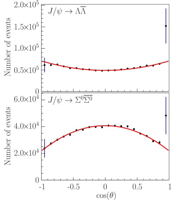
Figure 1: Angular distribution of the baryon for the ${J\!/\psi}$ decays into $\Lambda\overline{\Lambda}$ (upper panel) and $\Sigma^{0}\overline{\Sigma}{}^{0}$ (lower panel).

Figure 1 and 2 show BESIII data brdata on the angular distribution of the four decays: ${J\!/\psi}\to\Lambda\overline{\Lambda}$, ${J\!/\psi}\to\Sigma^{0}\overline{\Sigma}{}^{0}$, and ${\psi(2S)}\to\Lambda\overline{\Lambda}$, ${\psi(2S)}\to\Sigma^{0}\overline{\Sigma}{}^{0}$ respectively.

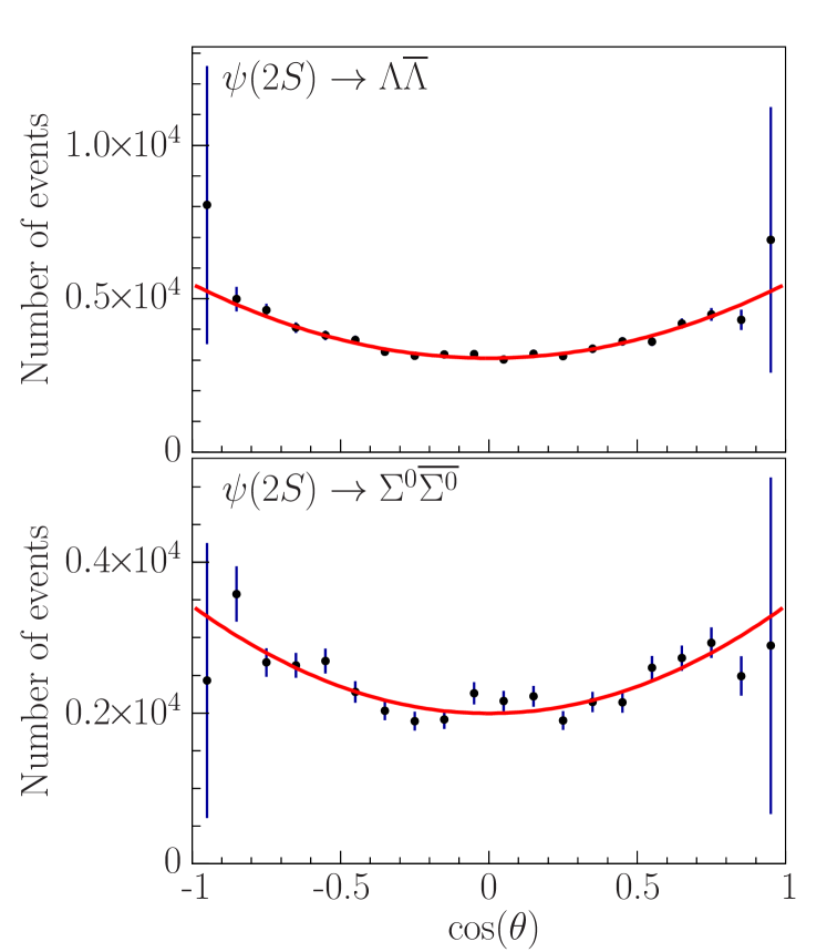
Figure 2: Angular distribution of the baryon for the ${\psi(2S)}$ decays into $\Lambda\overline{\Lambda}$ (upper panel) and $\Sigma^{0}\overline{\Sigma}{}^{0}$ (lower panel).

II Amplitudes and branching ratios

The Feynman amplitude for the decay $\psi\to B\overline{B}$ can be written in terms of the strong magnetic and Dirac FFs as

$$\mathcal{M}_{\psi\to B\overline{B}}=-i\epsilon_{\psi}^{\mu}\,\overline{u}(p_{1})\Gamma_{\mu}v(p_{2})$$

where the matrix $\Gamma_{\mu}$ is defined in Eq. (5), $\epsilon_{\psi}^{\mu}$ is the polarization vector of the $\psi$ meson, and the four-momenta follow the labelling of Eq. (4). The branching ratio (BR) is given by the standard form for the two-body decay

$$\mathcal{B}_{\psi\to B\overline{B}}={1\over\Gamma_{\psi}}\frac{1}{8\pi}\overline{\left|\mathcal{M}_{\psi\to B\overline{B}}\right|^{2}}\frac{\left|\vec{p}_{1}\right|}{M_{\psi}^{2}}\,,$$

where $\Gamma_{\psi}$ is the total width of the $\psi$ meson. Using the mean value of the modulus squared of the amplitude, written in terms of the Sachs couplings,

$$\overline{\left|\mathcal{M}_{\psi\to B\overline{B}}\right|^{2}} \!=\! \frac{4}{3}M_{\psi}^{2}\left(|g_{M}^{B}|^{2}+\frac{2M_{B}^{2}}{M_{\psi}^{2}}|g_{E}^{B}|^{2}\right)\,.$$

we obtain the BR

$$\mathcal{B}_{\psi\to B\overline{B}}=\frac{M_{\psi}\beta}{12\pi\Gamma_{\psi}}\left(|g_{M}^{B}|^{2}+\frac{2M_{B}^{2}}{M_{\psi}^{2}}|g_{E}^{B}|^{2}\right).$$ (1)

Since it does not depend on $\alpha_{B}$, it cannot be used to determine the polarization parameter.
The previous expression for the BR can be written as the sum of the moduli squared of two amplitudes

$${\mathcal{B}}_{\psi\to B\overline{B}}=\left|A^{B}_{M}\right|^{2}+\left|A^{B}_{E}\right|^{2}\,,$$ (2)

where, comparing with Eq. (1),

$$A^{B}_{M}=\sqrt{\frac{M_{\psi}\beta}{12\pi\Gamma_{\psi}}}\,g_{M}^{B}\,,\ \ A^{B}_{E}=\sqrt{\frac{M_{\psi}\beta}{6\pi\Gamma_{\psi}}}\frac{M_{B}}{M_{\psi}}\,g_{E}^{B}\,.$$

It follows that the polarization parameter of Eq. (6) can be also written as

$$\alpha_{B}={1-2|A_{E}^{B}|^{2}/|A_{M}^{B}|^{2}\over 1+2|A_{E}^{B}|^{2}/|A_{M}^{B}|^{2}}\,.$$

III Effective model

The SU(3) baryon octet states can be described by a matrix notation as follows ottetto

$$O_{B} = \begin{pmatrix}\Lambda/\sqrt{6}+\Sigma^{0}/\sqrt{2}&\Sigma^{+}&p\\ \Sigma^{-}&\Lambda/\sqrt{6}-\Sigma^{0}/\sqrt{2}&n\\ \Xi^{-}&\Xi^{0}&-2\Lambda/\sqrt{6}\end{pmatrix}\,,$$

$$O_{\overline{B}} = \begin{pmatrix}\overline{\Lambda}/\sqrt{6}+\overline{\Sigma}^{0}/\sqrt{2}&\overline{\Sigma}^{+}&\overline{\Xi}^{+}\\ \overline{\Sigma}^{-}&\overline{\Lambda}/\sqrt{6}-\overline{\Sigma}^{0}/\sqrt{2}&\overline{\Xi}^{0}\\ \overline{p}&\overline{n}&-2\overline{\Lambda}/\sqrt{6}\\ \end{pmatrix}\,,$$

where the first matrix is for baryons and the latter for antibaryons. We can consider the $J/\psi$ and $\psi(2S)$ mesons as SU(3) singlets. Following the SU(3) symmetry the level zero Lagrangian density should have the SU(3) invariant form $\mathcal{L}^{0}\propto{\ \rm Tr}(B\overline{B})$. Moreover, we consider two SU(3) breaking sources: the quark mass and the EM interaction. The first one can be parametrized by introducing the spurion matrix Zhu:2015bha

$$S_{m}={g_{m}\over 3}\begin{pmatrix}1&0&0\\ 0&1&0\\ 0&0&-2\\ \end{pmatrix}\,,$$

where $g_{m}$ is an effective coupling constant. This matrix describes the mass breaking effect due to the mass difference between $s$ and, $u$ and $d$ quarks, where the SU(2) isospin symmetry is assumed, so that $m_{u}=m_{d}$. This SU(3) breaking is proportional to the 8^th Gell-Mann matrix $\lambda_{8}$. The EM breaking effect is related to the fact that the photon coupling to quarks, described by the four-current

$${1\over 2}\overline{q}\gamma^{\mu}\left(\lambda_{3}+\lambda_{8}/\sqrt{3}\right)q\,,$$

is proportional to the electric charge. This effect can be parametrized using the following spurion matrix

$$S_{e}={g_{e}\over 3}\begin{pmatrix}2&0&0\\ 0&-1&0\\ 0&0&-1\\ \end{pmatrix}\,,$$

where $g_{e}$ is an EM effective coupling constant.
The most general SU(3) invariant effective Lagrangian density is given by Zhu:2015bha

$$\mathcal{L} = g\,{\rm Tr}(OO_{\overline{B}})+d\,{\rm Tr}\big{(}\{O,O_{\overline{B}}\}S_{e}\big{)}+f\,{\rm Tr}\big{(}[OO_{\overline{B}}]S_{e}\big{)}$$

$$+d^{\prime}\,{\rm Tr}\big{(}\{O,O_{\overline{B}}\}S_{m}\big{)}+f^{\prime}\,{\rm Tr}\big{(}[O,O_{\overline{B}}]S_{m}\big{)}\,,$$

where $g$, $d$, $f$, $d^{\prime}$ and $f^{\prime}$ are coupling constants. We can extract the Lagrangians describing the $J/\psi$ and $\psi(2S)$ decays into $\Lambda\overline{\Lambda}$ and $\Sigma^{0}\overline{\Sigma}^{0}$

$${\mathcal{L}}_{\Sigma^{0}\overline{\Sigma}{}^{0}}=(G_{0}+G_{1})\,\Sigma^{0}\overline{\Sigma}{}^{0}\,,\ {\mathcal{L}}_{\Lambda\overline{\Lambda}}=(G_{0}-G_{1})\,\Lambda\overline{\Lambda}\,,$$ (3)

where $G_{0}$ and $G_{1}$ are combinations of coupling constants, i.e.,

$$G_{0}=g\,,\hskip 28.45274ptG_{1}={d\over 3}\,(2g_{m}+g_{e})\,.$$

By using the same structure of Eq. (2), the BRs can be expressed in terms of electric and magnetic amplitudes as

$$\mathcal{B}_{\psi\to\Sigma^{0}\overline{\Sigma}^{0}} = |A_{E}^{\Sigma}|^{2}+|A_{M}^{\Sigma}|^{2}\,,$$

$$\mathcal{B}_{\psi\to\Lambda\overline{\Lambda}} = |A_{E}^{\Lambda}|^{2}+|A_{M}^{\Lambda}|^{2}\,.$$

Moreover, as obtained in Eq. (3), such amplitudes can be further decomposed as combinations of leading, $E_{0}$ and $M_{0}$, and sub-leading terms, $E_{1}$ and $M_{1}$, with opposite relative signs, i.e.,

$${{\mathcal{B}}}_{\psi\to\Sigma^{0}\overline{\Sigma}{}^{0}} = |E_{0}+E_{1}|^{2}+|M_{0}+M_{1}|^{2}$$

$$= |E_{0}|^{2}+|E_{1}|^{2}+2|E_{0}||E_{1}|\cos(\rho_{E})$$

$$+|M_{0}|^{2}+|M_{1}|^{2}+2|M_{0}||M_{1}|\cos(\rho_{M})\,,$$

$${{\mathcal{B}}}_{\psi\to\Lambda\overline{\Lambda}} = |E_{0}-E_{1}|^{2}+|M_{0}-M_{1}|^{2}$$

$$= |E_{0}|^{2}+|E_{1}|^{2}-2|E_{0}||E_{1}|\cos(\rho_{E})$$

$$+|M_{0}|^{2}+|M_{1}|^{2}-2|M_{0}||M_{1}|\cos(\rho_{M})\,,$$

where $\rho_{E}$ and $\rho_{M}$ are the phases of the ratios $E_{0}/E_{1}$ and $M_{0}/M_{1}$.

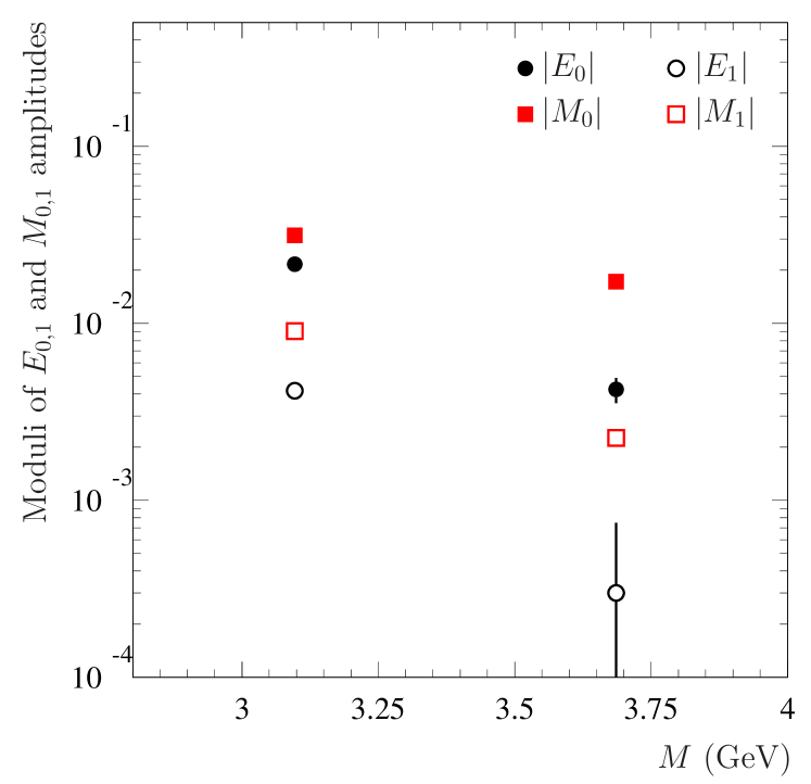
Figure 3: Moduli of the parameters from table 2 as a function of the charmonium state mass $M$.

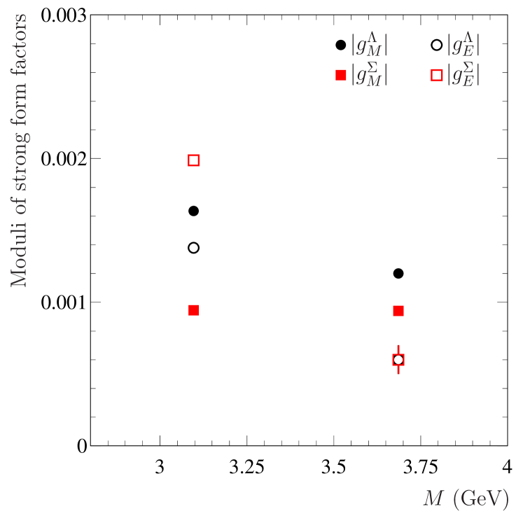
Figure 4: Moduli of the parameters from table 3 as a function of the charmonium state mass $M$.

Table 1: Branching ratios and polarization parameters from Ref. brdata . In particular the value of $\alpha_{B}$ for the decay ${J\!/\psi}\to\Lambda\overline{\Lambda}$ is from Ref. Ablikim:2018zay .

Decay	BR	Pol. par. $\alpha_{B}$
$J/\psi\to\Sigma^{0}\overline{\Sigma}^{0}$	$(11.64\pm 0.04)\times 10^{-4}$	$-0.449\pm 0.020$
$J/\psi\to\Lambda\overline{\Lambda}$	$(19.43\pm 0.03)\times 10^{-4}$	$0.461\pm 0.009$
$\psi(2S)\to\Sigma^{0}\overline{\Sigma}^{0}$	$(2.44\pm 0.03)\times 10^{-4}$	$0.71\pm 0.11$
$\psi(2S)\to\Lambda\overline{\Lambda}$	$(3.97\pm 0.03)\times 10^{-4}$	$0.824\pm 0.074$

Table 2: Moduli of the leading and sub-leading amplitudes.

Ampl.	$J/\psi$	$\psi(2S)$
$|E_{0}|$	$(2.16\pm 0.02)\times 10^{-2}$	$(0.42\pm 0.07)\times 10^{-2}$
$|E_{1}|$	$(0.42\pm 0.02)\times 10^{-2}$	$(0.03\pm 0.05)\times 10^{-2}$
$|M_{0}|$	$(3.15\pm 0.02)\times 10^{-2}$	$(1.72\pm 0.02)\times 10^{-2}$
$|M_{1}|$	$(0.90\pm 0.02)\times 10^{-2}$	$(0.23\pm 0.02)\times 10^{-2}$

Table 3: Moduli of the strong Sachs FFs.

FFs	$J/\psi$	$\psi(2S)$
$|g_{E}^{\Sigma}|$	$(1.99\pm 0.04)\times 10^{-3}$	$(0.6\pm 0.1)\times 10^{-3}$
$|g_{M}^{\Sigma}|$	$(0.94\pm 0.02)\times 10^{-3}$	$(0.94\pm 0.02)\times 10^{-3}$
$|g_{E}^{\Lambda}|$	$(1.37\pm 0.04)\times 10^{-3}$	$(0.6\pm 0.1)\times 10^{-3}$
$|g_{M}^{\Lambda}|$	$(1.64\pm 0.03)\times 10^{-3}$	$(1.20\pm 0.02)\times 10^{-3}$

IV Results

In this work we have used data from precise measurements brdata ; Ablikim:2018zay of the BRs and polarization parameters, reported in table 1, based on events collected with the BESIII detector at the BEPCII collider. These data are in agreement with the results of other experiments Ablikim:2012pj ; Aubert:2007uf ; Pedlar:2005px ; Ablikim:2006aw ; Dobbs:2014ifa . Since for each charmonium state we have six free parameters (four moduli and two relative phases) and only four constrains (two BRs and two polarization parameters), we have to fix the relative phases $\rho_{E}$ and $\rho_{M}$. The values $\rho_{E}=0$ and $\rho_{M}=\pi$ appear as phenomenologically favored by the data themselves. Indeed, (largely) different phases would give negative, and hence unphysical, values for the moduli $|E_{0}|$, $|E_{1}|$, $|M_{0}|$ and $|M_{1}|$. Moreover, as shown in Fig. 5, where the four moduli for $J/\psi$ and $\psi(2S)$ are represented as functions of the phases with $\rho_{E}\in[-\pi/2,\pi/2]$ and $\rho_{M}\in[\pi/2,3\pi/2]$, the obtained results are quite stable, and the central values $\rho_{E}=0$, $\rho_{M}=\pi$ maximise the hierarchy between the moduli of leading, $E_{0}$ and $M_{0}$, and sub-leading amplitudes, $E_{1}$ and $M_{1}$.

Figure 5: Red and black bands represent moduli of leading and sub-leading amplitudes respectively. The vertical width indicates the error. Top left: moduli of amplitudes $E_{0}$ and $E_{1}$ of $J/\psi$. Top right: moduli of amplitudes $M_{0}$ and $M_{1}$ of $J/\psi$. Bottom left: moduli of amplitudes $E_{0}$ and $E_{1}$ of $\psi(2S)$. Bottom right: moduli of amplitudes $M_{0}$ and $M_{1}$ of $\psi(2S)$.

Such values for $|E_{0}|$, $|E_{1}|$, $|M_{0}|$ and $|M_{1}|$ are reported in table 2 and shown in Fig. 3. The corresponding values of $|g_{E}|$, $|g_{M}|$ are reported in table 3 and shown in Fig. 4. The large sub-leading ${J\!/\psi}$ amplitudes $|E_{1}|$, $|M_{1}|$ (see table 2 and Fig. 3) are responsible for the inversion of the $|g_{E}^{B}|$, $|g_{M}^{B}|$ hierarchy (see Fig. 4 and table 3).

V Conclusions

Different $\Lambda$ and $\Sigma^{0}$ angular distributions can be explained using an effective model with the SU(3)-driven Lagrangian

$$\mathcal{L}_{\Sigma^{0}\overline{\Sigma}{}^{0}+\Lambda\overline{\Lambda}}=(G_{0}+G_{1})\Sigma^{0}\overline{\Sigma}^{0}+(G_{0}-G_{1})\Lambda\overline{\Lambda}\,.$$

The interplay between leading $G_{0}$ and sub-leading $G_{1}$ contributions to the decay amplitudes determines signs and values of polarization parameters $\alpha_{B}$.
In particular the different behavior of the ${J\!/\psi}\to\Sigma^{0}\overline{\Sigma}{}^{0}$ angular distribution is due to the large values of the sub-leading amplitudes $|E_{1}|$ and $|M_{1}|$. It implies that the SU(3) mass breaking and EM effects, which are responsible for these amplitudes, play a different role in the dynamics of the ${J\!/\psi}$ and ${\psi(2S)}$ decays.
It is interesting to notice that angular distributions of $\Sigma^{0}(1385)$ and $\Sigma^{\pm}(1385)$, measured by BESIII Ablikim:2016sjb ; Ablikim:2016iym , show the same $\Sigma^{0}$ behavior.
The process $e^{+}e^{-}\to{J\!/\psi}\to\Sigma^{+}\overline{\Sigma}^{-}$ is currently under investigation ref.p , the behavior of its angular distribution would add important pieces of information to the knowledge of the $J\!/\psi$ decay mechanism.

Appendix A Production cross section

We consider the decay of a charmonium state, a $c\overline{c}$ vector meson $\psi$, produced via $e^{+}e^{-}$ annihilation, into a pair baryon-antibaryon $B\overline{B}$, i.e., the process

$$e^{-}(k_{1})+e^{+}(k_{2})\to\psi(q)\to B(p_{1})+\overline{B}(p_{2})\,,$$ (4)

where in parentheses are shown the 4-momenta.

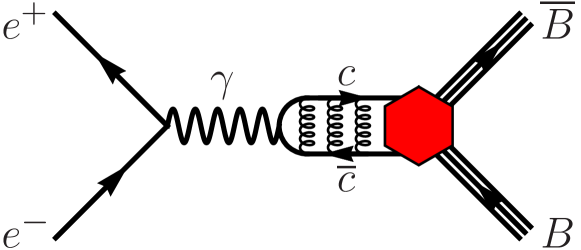
Figure 6: Feynman diagram of the process $e^{+}e^{-}\to\psi\to B\overline{B}$, the red hexagon represents the $\psi B\overline{B}$ coupling.

The Feynman diagram is shown in Fig. 6 and the corresponding amplitude is

$$\mathcal{M}_{e^{+}e^{-}\to\psi\to B\overline{B}}=-ie^{2}J_{B}^{\mu}\ D_{\psi}\!\left(q^{2}\right)\,\overline{v}(k_{2})\gamma_{\mu}u(k_{1})\,,$$

where $J_{B}^{\mu}=\overline{u}(p_{1})\Gamma^{\mu}v(p_{2})$ is the baryonic four-current, $D_{\psi}\left(q^{2}\right)$ is the $\psi$ propagator, which includes the $\gamma$-$\psi$ electromagnetic (EM) coupling, and $\overline{v}(k_{2})\gamma_{\mu}u(k_{1})$ is the leptonic four-current, the four-momenta follow the labelling of Eq. (4). The $\Gamma^{\mu}$ matrix can be written as dirac-pauli

$$\Gamma^{\mu}=\gamma^{\mu}f_{1}^{B}+\frac{i\sigma^{\mu\nu}q_{\nu}}{2M_{B}}\,f_{2}^{B}\,,$$ (5)

where $M_{B}$ is the baryon mass and, $f_{1}^{B}$ and $f_{2}^{B}$ are constant form factors (FFs) that we call “strong” Dirac and Pauli couplings, they weight the vector and tensor part of the $\psi B\overline{B}$ vertex . We can introduce the strong electric and magnetic Sachs couplings sachs

$$g_{E}^{B}=f_{1}^{B}+\frac{M_{\psi}^{2}}{4M_{B}^{2}}f_{2}^{B}\,,\hskip 14.22636ptg_{M}^{B}=f_{1}^{B}+f_{2}^{B}\,,$$

that have the same structure of the EM Sachs FFs Claudson:1981fj , $M_{\psi}$ is the mass of the charmonium state. The four quantities $f_{1}^{B}$, $f_{2}^{B}$, $g_{E}^{B}$ and $g_{M}^{B}$ are in general complex numbers. The differential cross section of the process $e^{+}e^{-}\to\psi\to B\overline{B}$, in the $e^{+}e^{-}$ center of mass frame, in terms of the two Sachs couplings, reads

$$\frac{d\sigma}{d\cos\theta}=\frac{\pi\alpha^{2}\beta}{2M_{\psi}^{2}}\left(\left|g_{M}^{B}\right|^{2}+\frac{4M_{B}^{2}}{M_{\psi}^{2}}\left|g_{E}^{B}\right|^{2}\right)\!\Big{(}1+\alpha_{B}\cos^{2}\theta\Big{)}\,,$$

where

$$\beta=\sqrt{1-{4M_{B}^{2}\over M_{\psi}^{2}}}$$

is the velocity of the out-going baryon at the $\psi$ mass, $\theta$ is the scattering angle, and the polarization parameter $\alpha_{B}$ is given by

$$\alpha_{B}=\frac{M_{\psi}^{2}\left|g_{M}^{B}\right|^{2}-4M_{B}^{2}|g_{E}^{B}|^{2}}{M_{\psi}^{2}\left|g_{M}^{B}\right|^{2}+4M_{B}^{2}\left|g_{E}^{B}\right|^{2}}\,,$$ (6)

$\alpha_{B}\in[-1,1]$. It depends only on the modulus of the ratio ${g_{E}^{B}}/{g_{M}^{B}}$, e.g., Fig. 7 shows the behavior of $\alpha_{\Lambda}$ in the case of $\psi={J\!/\psi}$ as a function of $|g_{E}^{\Lambda}|/|g_{M}^{\Lambda}|$. The strong Sachs and, Dirac and Pauli couplings are related through $\alpha_{B}$. Let us consider three peculiar cases. With maximum positive polarization, $\alpha_{B}=1$, the strong electric Sachs coupling vanishes, i.e.,

$$\alpha_{B}=1\ \ \to\ \ g_{E}^{B}=0\,,\ \ f_{1}^{B}=-\frac{M_{\psi}^{2}}{4M_{B}^{2}}f_{2}^{B}\,,$$

$$g_{M}^{B}=f_{1}^{B}\left(1-\frac{4M_{B}^{2}}{M_{\psi}^{2}}\right)=f_{2}^{B}\left(1-\frac{M_{\psi}^{2}}{4M_{B}^{2}}\right)\,,$$

the relative phase between $f_{1}^{B}$ and $f_{2}^{B}$ is $i\pi$, and the ratio of the moduli is $M_{\psi}^{2}/(4M_{B}^{2})$.

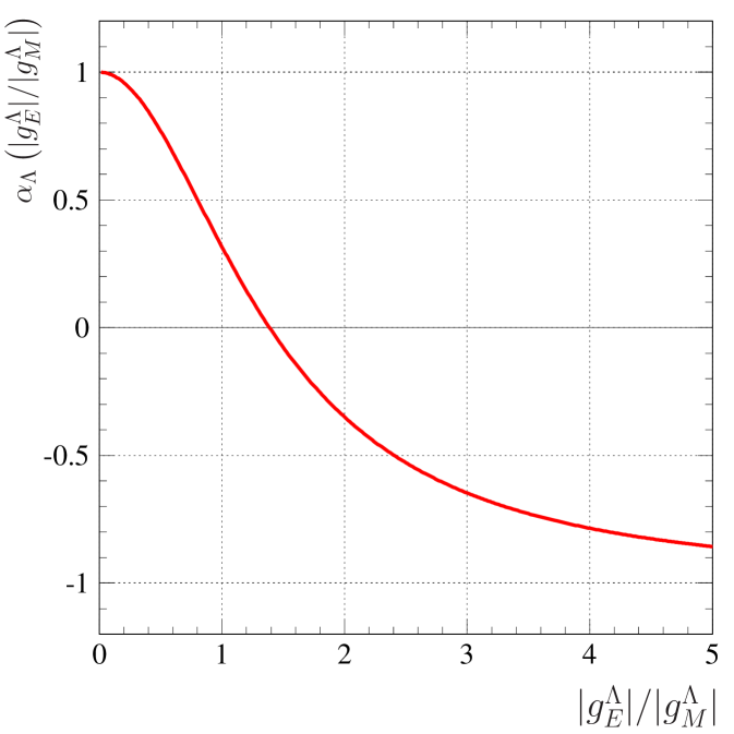
Figure 7: Polarization parameter $\alpha_{\Lambda}$ for the $\psi=J/\psi$ as a function of the ratio $|g_{E}^{\Lambda}|/|g_{M}^{\Lambda}|$. The masses are from Ref. pdg .

With maximum negative polarization we have

$$\alpha_{B}=-1\ \ \to\ \ g_{M}^{B}=0\,,\ \ f_{1}^{B}=-f_{2}^{B}\,,$$

$$g_{E}^{B}=f_{1}^{B}\left(1-\frac{M_{\psi}^{2}}{4M_{B}^{2}}\right)=f_{2}^{B}\left(\frac{M_{\psi}^{2}}{4M_{B}^{2}}-1\right)\,,$$

in this case the strong magnetic Sachs coupling vanishes, the relative phase between $f_{1}^{B}$ and $f_{2}^{B}$ is $-i\pi$ and the ratio of the moduli is one.
Finally in the case with no polarization, $\alpha_{B}=0$, we obtain the modulus of the ratio between the Sachs couplings

$$\alpha_{B}=0\ \ \to\ \ \frac{|g_{E}^{B}|}{|g_{M}^{B}|}=\frac{M_{\psi}}{2M_{B}}\,.$$

References

(1)
S. J. Brodsky and G. P. Lepage,
Phys. Rev. D 24 (1981) 2848.
(2)
M. Ablikim et al. [BES Collaboration],
Phys. Lett. B 632 (2006) 181
[hep-ex/0506020].
(3)
M. Ablikim et al. [BESIII Collaboration],
Phys. Rev. D 95 (2017) no.5, 052003
[arXiv:1701.07191 [hep-ex]].
(4) M. Gell-Mann,
Phys. Rev. 125 (1962) 1067.
(5)
K. Zhu, X. H. Mo and C. Z. Yuan,
Int. J. Mod. Phys. A 30 (2015) no.25, 1550148
[arXiv:1505.03930 [hep-ph]].
(6)
M. Ablikim et al. [BESIII Collaboration],
arXiv:1808.08917 [hep-ex].
(7)
M. Ablikim et al. [BESIII Collaboration],
Chin. Phys. C 37 (2013) 063001
[arXiv:1209.6199 [hep-ex]].
(8)
B. Aubert et al. [BaBar Collaboration],
Phys. Rev. D 76 (2007) 092006
[arXiv:0709.1988 [hep-ex]].
(9)
T. K. Pedlar et al. [CLEO Collaboration],
Phys. Rev. D 72 (2005) 051108
[hep-ex/0505057].
(10)
M. Ablikim et al. [BES Collaboration],
Phys. Lett. B 648 (2007) 149
[hep-ex/0610079].
(11)
S. Dobbs, A. Tomaradze, T. Xiao, K. K. Seth and G. Bonvicini,
Phys. Lett. B 739 (2014) 90
[arXiv:1410.8356 [hep-ex]].
(12)
M. Ablikim et al. [BESIII Collaboration],
Phys. Lett. B 770 (2017) 217
[arXiv:1612.08664 [hep-ex]].
(13)
M. Ablikim et al. [BESIII Collaboration],
Phys. Rev. D 93 (2016) no.7, 072003
[arXiv:1602.06754 [hep-ex]].
(14)
L. Yan (BESIII Collaboration), private communication.
(15)
G. Salzman,
Phys. Rev. 99 (1955) 973.
(16) F. J. Ernst, R. G. Sachs and K. C. Wali,
Phys. Rev. 119 (1960) 1105.
(17)
M. Claudson, S. L. Glashow and M. B. Wise,
Phys. Rev. D 25 (1982) 1345.
doi:10.1103/PhysRevD.25.1345
(18)
C. Patrignani et al. [Particle Data Group],
Chin. Phys. C 40 (2016) no.10, 100001.