Abstract

Ensembles of deep neural networks significantly improve generalization accuracy. However, training neural network ensembles requires a large amount of computational resources and time. State-of-the-art approaches either train all networks from scratch leading to prohibitive training cost that allows only very small ensemble sizes in practice, or generate ensembles by training a monolithic architecture, which results in lower model diversity and decreased prediction accuracy. We propose MotherNets to enable higher accuracy and practical training cost for large and diverse neural network ensembles: A MotherNet captures the structural similarity across some or all members of a deep neural network ensemble which allows us to share data movement and computation costs across these networks. We first train a single or a small set of MotherNets and, subsequently, we generate the target ensemble networks by transferring the function from the trained MotherNet(s). Then, we continue to train these ensemble networks, which now converge drastically faster compared to training from scratch. MotherNets handle ensembles with diverse architectures by clustering ensemble networks of similar architecture and training a separate MotherNet for every cluster. MotherNets also use clustering to control the accuracy vs. training cost tradeoff. We show that compared to state-of-the-art approaches such as Snapshot Ensembles, Knowledge Distillation, and TreeNets, MotherNets provide a new Pareto frontier for the accuracy-training cost tradeoff. Crucially, training cost and accuracy improvements continue to scale as we increase the ensemble size (2 to 3 percent reduced absolute test error rate and up to 35 percent faster training compared to Snapshot Ensembles). We verify these benefits over numerous neural network architectures and large data sets.

1 Introduction

Neural network ensembles. Various applications increasingly use ensembles of multiple neural networks to scale the representational power of their deep learning pipelines. For example, deep neural network ensembles predict relationships between chemical structure and reactivity Agrafiotis et al. (2002), segment complex images with multiple objects Ju et al. (2017), and are used in zero-shot as well as multiple choice learning Guzman-Rivera et al. (2014); Ye & Guo (2017). Further, several winners and top performers on the ImageNet challenge are ensembles of neural networks Lee et al. (2015a); Russakovsky et al. (2015). Ensembles function as collections of experts and have been shown, both theoretically and empirically, to improve generalization accuracy Drucker et al. (1993); Dietterich (2000); Granitto et al. (2005); Huggins et al. (2016); Ju et al. (2017); Lee et al. (2015a); Russakovsky et al. (2015); Xu et al. (2014). For instance, by combining several image classification networks on the CIFAR-10, CIFAR-100, and SVHN data sets, ensembles can reduce the misclassification rate by up to $20$ percent, e.g., from $6$ percent to $4.5$ percent for ensembles of ResNets on CIFAR-10 Huang et al. (2017a); Ju et al. (2017).

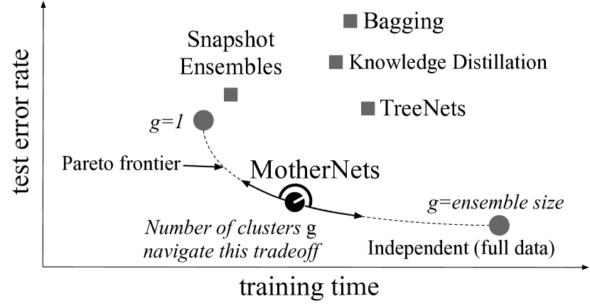
Figure 1: MotherNets establish a new Pareto frontier for the accuracy-training time tradeoff as well as navigate this tradeoff.

The growing training cost. Training ensembles of multiple deep neural networks takes a prohibitively large amount of time and computational resources. Even on high-performance hardware, a single deep neural network may take several days to train and this training cost grows linearly with the size of the ensemble as every neural network in the ensemble needs to be trained Szegedy et al. (2015); He et al. (2016); Huang et al. (2017b; a). This problem persists even in the presence of multiple machines. This is because the holistic cost of training, in terms of buying or renting out these machines through a cloud service provider, still increases linearly with the ensemble size. The rising training cost is a bottleneck for numerous applications, especially when it is critical to quickly incorporate new data and to achieve a target accuracy. For instance, in one use case, where deep learning models are applied to detect Diabetic Retinopathy (a leading cause of blindness), newly labelled images become available every day. Thus, incorporating new data in the neural network models as quickly as possible is crucial in order to enable more accurate diagnosis for the immediately next patient Gulshan et al. (2016).

Table 1: Existing approaches to train ensembles of deep neural networks are limited in speed, accuracy, diversity, and size.

	Fast	High	Diverse	Large
	train.	acc.	arch.	size
Full data	$\times$			$\times$
Bagging	$\sim$	$\times$		$\times$
Knowledge Dist.	$\sim$	$\times$		$\times$
TreeNets	$\sim$	$\sim$	$\times$	$\times$
Snapshot Ens.			$\times$	$\times$
MotherNets

Problem 1: Restrictive ensemble size. Due to this prohibitive training cost, researchers and practitioners can only feasibly train and employ small ensembles Szegedy et al. (2015); He et al. (2016); Huang et al. (2017b; a). In particular, neural network ensembles contain drastically fewer individual models when compared with ensembles of other machine learning methods. For instance, random decision forests, a popular ensemble algorithm, often has several hundreds of individual models (decision trees), whereas state-of-the-art ensembles of deep neural networks consist of around five networks He et al. (2016); Huang et al. (2017b; a); Oshiro et al. (2012); Szegedy et al. (2015). This is restrictive since the generalization accuracy of an ensemble increases with the number of well-trained models it contains Oshiro et al. (2012); Bonab & Can (2016); Huggins et al. (2016). Theoretically, for best accuracy, the size of the ensemble should be at least equal to the number of class labels, of which there could be thousands in modern applications Bonab & Can (2016).

Additional problems: Speed, accuracy, and diversity. Typically, every deep neural network in an ensemble is initialized randomly and then trained individually using all training data (full data), or by using a random subset of the training data (i.e., bootstrap aggregation or bagging) Ju et al. (2017); Lee et al. (2015a); Moghimi & Vasconcelos (2016). This requires a significant amount of processing time and computing resources that grow linearly with the ensemble size.

To alleviate this linear training cost, two techniques have been recently introduced that generate a $k$ network ensemble from a single network: Snapshot Ensembles and TreeNets. Snapshot Ensembles train a single network and use its parameters at $k$ different points of the training process to instantiate $k$ networks that will form the target ensemble Huang et al. (2017a). Snapshot Ensembles vary the learning rate in a cyclical fashion, which enables the single network to converge to $k$ local minima along its optimization path. TreeNets also train a single network but this network is designed to branch out into $k$ sub-networks after the first few layers. Effectively every sub-network functions as a separate member of the target ensemble Lee et al. (2015b).

While these approaches do improve training time, they also come with two critical problems. First, the resulting ensembles are less accurate because they are less diverse compared to using $k$ different and individually trained networks. Second, these approaches cannot be applied to state-of-the-art diverse ensembles. Such ensembles may contain arbitrary neural network architectures with structural differences to achieve increased accuracy (for instance, such as those used in the ImageNet competitions Lee et al. (2015a); Russakovsky et al. (2015)).

Knowledge Distillation provides a middle ground between separate training and ensemble generation approaches Hinton et al. (2015). With Knowledge Distillation, an ensemble is trained by first training a large generalist network and then distilling its knowledge to an ensemble of small specialist networks that may have different architectures (by training them to mimic the probabilities produced by the larger network) Hinton et al. (2015); Li & Hoiem (2017). However, this approach results in limited improvement in training cost as distilling knowledge still takes around $70$ percent of the time needed to train from scratch. Even then, the ensemble networks are still closely tied to the same large network that they are distilled from. The result is significantly lower accuracy and diversity when compared to ensembles where every network is trained individually Hinton et al. (2015); Li & Hoiem (2017).

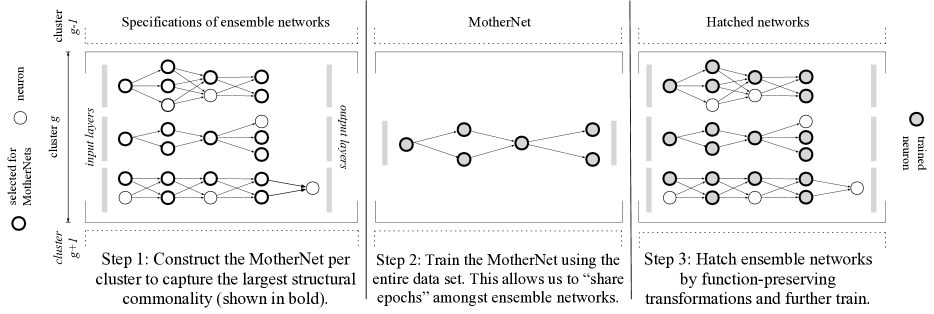
Figure 2: MotherNets train an ensemble of neural networks by first training a set of MotherNets and transferring the function to the ensemble networks. The ensemble networks are then further trained converging significantly faster than training individually.

MotherNets. We propose MotherNets, which enable rapid training of large feed-forward neural network ensembles. The core benefits of MotherNets are depicted in Table 1. MotherNets provide: (i) lower training time and better generalization accuracy than existing fast ensemble training approaches and (ii) the capacity to train large ensembles with diverse network architectures.

Figure 2 depicts the core intuition behind MotherNets: A MotherNet is a network that captures the maximum structural similarity between a cluster of networks (Figure 2 Step (1)). An ensemble may consist of one or more clusters; one MotherNet is constructed per cluster. Every MotherNet is trained to convergence using the full data set (Figure 2 Step (2)). Then, every target network in the ensemble is hatched from its MotherNet using function-preserving transformations (Figure 2 Step (3)) ensuring that knowledge from the MotherNet is transferred to every network. The ensemble networks are then trained. They converge significantly faster compared to training from scratch (within tens of epochs).

The core technical intuition behind the MotherNets design is that it enables us to “share epochs” between the ensemble networks. At a lower level what this means is that the networks implicitly share part of the data movement and computation costs that manifest during training over the same data. This design draws intuition from systems techniques such as “shared scans” in data systems where many queries share data movement and computation for part of a scan over the same data Harizopoulos et al. (2005); Zukowski et al. (2007); Qiao et al. (2008); Arumugam et al. (2010); Candea et al. (2011); Giannikis et al. (2012); Psaroudakis et al. (2013); Giannikis et al. (2014); Kester et al. (2017).

Accuracy-training time tradeoff. MotherNets do not train each network individually but “source” all networks from the same set of “seed” networks instead. This introduces some reduction in diversity and accuracy compared to an approach that trains all networks independently. There is no way around this. In practice, there is an intrinsic tradeoff between ensemble accuracy and training time. All existing approaches are affected by this and their design decisions effectively place them at a particular balance within this tradeoff Guzman-Rivera et al. (2014); Lee et al. (2015a); Huang et al. (2017a).

We show that MotherNets, strike a superior balance between accuracy and training time than all existing approaches. In fact, we show that MotherNets establish a new Pareto frontier for this tradeoff and that we can navigate this tradeoff. To achieve this, MotherNets cluster ensemble networks (taking into account both the topology and the architecture class) and train a separate MotherNet for each cluster. The number of clusters used (and thus the number of MotherNets) is a knob that helps navigate the training time vs. accuracy tradeoff. Figure 1 depicts visually the new tradeoff achieved by MotherNets.

Contributions. We describe how to construct MotherNets in detail and how to trade accuracy for speed. Then through a detailed experimental evaluation with diverse data sets and architectures we demonstrate that MotherNets bring three benefits: (i) MotherNets establish a new Pareto frontier of the accuracy-training time tradeoff providing up to $2$ percent better absolute test error rate compared to fast ensemble training approaches at comparable or less training cost. (ii) MotherNets allow robust navigation of this new Pareto frontier of the tradeoff between accuracy and training time. (iii) MotherNets enable scaling of neural network ensembles to large sizes (100s of models) with practical training cost and increasing accuracy benefits.

We provide a web-based interactive demo as an additional resource to help in understanding the training process in MotherNets: http://daslab.seas.harvard.edu/mothernets/.

2 Rapid Ensemble Training

Definition: MotherNet. Given a cluster of $k$ neural networks $C=\{N_{1},N_{2},\dots N_{k}\}$, where $N_{i}$ denotes the $i$-th neural network in $C$, the MotherNet $M_{c}$ is defined as the largest network from which all networks in $C$ can be obtained through function-preserving transformations. MotherNets divide an ensemble into one or more such network clusters and construct a separate MotherNet for each.

Constructing a MotherNet for fully-connected networks. Assume a cluster $C$ of fully-connected neural networks. The input and the output layers of $M_{c}$ have the same structure as all networks in $C$, since they are all trained for the same task. $M_{c}$ is initialized with as many hidden layers as the shallowest network in $C$. Then, we construct the hidden layers of $M_{c}$ one-by-one going from the input to the output layer. The structure of the $i$-th hidden layer of $M_{c}$ is the same as the $i$-th hidden layer of the network in $C$ with the least number of parameters at the $i$-th layer. Figure 2 shows an example of how this process works for a toy ensemble of two three-layered and one four-layered neural networks. Here, the MotherNet is constructed with three layers. Every layer has the same structure as the layer with the least number of parameters at that position (shown in bold in Figure 2 Step (1)). In Appendix A we also include a pseudo-code description of this algorithm.

Constructing a MotherNet for convolutional networks. Convolutional neural network architectures consist of blocks of one or more convolutional layers separated by pooling layers He et al. (2016); Shazeer et al. (2017); Simonyan & Zisserman (2015); Szegedy et al. (2015). These blocks are then followed by another block of one or more fully-connected layers. For instance, VGGNets are composed of five blocks of convolutional layers separated by max-pooling layers, whereas, DenseNets consist of four blocks of densely connected convolutional layers. For convolutional networks, we construct the MotherNet $M_{c}$ block-by-block instead of layer-by-layer. The intuition is that deeper or wider variants of such networks are created by adding or expanding layers within individual blocks instead of adding them all at the end of the network. For instance, VGG-C (with 16 convolutional layers) is obtained by adding one layer to each of the last three blocks of VGG-B (with 13 convolutional layers) Simonyan & Zisserman (2015). To construct the MotherNet for every block, we select as many convolutional layers to include in the MotherNet as the network in $C$ with the least number of layers in that block. Every layer within a block is constructed such that it has the least number of filters and the smallest filter size of any layer at the same position within that block. An example of this process is shown in Figure 3. Here, we construct a MotherNet for three convolutional neural networks block-by-block. For instance, in the first block, we include one convolutional layer in the MotherNet having the smallest filter width and the least number of filters (i.e., 3 and 32 respectively). In Appendix A we also include a pseudo-code description of this algorithm.

Constructing MotherNets for ensembles of neural networks with different sizes and topologies. By construction, the overall size and topology (sequence of layer sizes) of a MotherNet is limited by the smallest network in its cluster. If we were to assign a single cluster to all networks in an ensemble that has a large difference in size and topology between the smallest and the largest networks, there will be a correspondingly large difference between at least one ensemble network and the MotherNet. This may lead to a scenario where the MotherNet only captures an insignificant amount of commonality. This would negatively affect performance as we would not be able to share significant computation and data movement costs across the ensemble networks. This property is directly correlated with the size of the MotherNet.

In order to maintain the ability to share costs in diverse ensembles, we partition such an ensemble into $g$ clusters, and for every cluster, we construct and train a separate MotherNet. To perform this clustering, the $m$ networks in the ensemble $E=\{N_{1},N_{2},\dots N_{m}\}$ are represented as vectors $E_{v}=\{V_{1},V_{2},\dots V_{m}\}$ such that $V_{i}^{j}$ stores the size of the $j$-th layer in $N_{i}$. These vectors are zero-padded to a length of $\max(\{|N_{1}|,|N_{2}|,\dots|N_{m}|\})$ (where $|N_{i}|$ is the number of layers in $N_{i}$). For convolutional neural networks, these vectors are created by first creating similarly zero-padded sub-vectors per block and then concatenating the sub-vectors to get the final vector. In this case, to fully represent convolutional layers, $V_{i}^{j}$ stores a 2-tuple of filter sizes and number of filters.

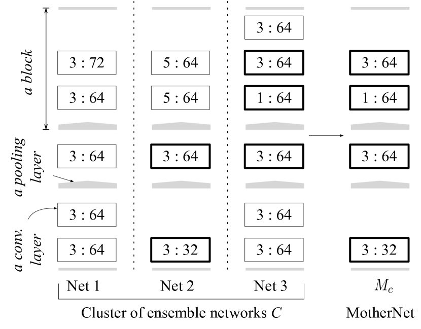
Figure 3: Constructing MotherNet for convolutional neural networks block-by-block. For each layer, we select the layer with the least number of parameters from the ensemble networks (shown in bold rectangles) (Notation: <filter_width>:<filter_number>).

Given a set of vectors $E_{v}$, we create $g$ clusters using the balanced K-means algorithm while minimizing the Levenshtein distance between the vector representation of networks in a cluster and its MotherNet Levenshtein (1966); MacQueen (1967). The Levenshtein or the edit distance between two vectors is the minimum number of edits – insertions, deletions, or substitutions – needed to transform one vector to another. By minimizing this distance, we ensure that, for every cluster, the ensemble networks can be obtained from their cluster’s MotherNet with the minimal amount of edits constrained on $g$. During every iteration of the K-means algorithm, instead of computing centers of candidate clusters, we construct MotherNets corresponding to every cluster. Then, we use the edit distance between these MotherNets and all networks to perform cluster reassignments.

Constructing MotherNets for ensembles of diverse architecture classes. An individual MotherNet is built for a cluster of networks that belong to a single architecture class. Each architecture class has the property of function-preserving navigation. This is to say that given any member of this class, we can build another member of this class with more parameters but having the same function. Multiple types of neural networks fall under the same architecture class Cai et al. (2018). For instance, we can build a single MotherNet for ensembles of AlexNets, VGGNets, and Inception Nets as well as one for DenseNets and ResNets. To handle scenarios when an ensemble contains members from diverse architecture classes i.e., we cannot navigate the entire set of ensemble networks in a function-preserving manner, we build a separate MotherNet for each class (or a set of MotherNets if each class also consists of networks of diverse sizes).

Overall, the techniques described in the previous paragraphs allow us to create $g$ MotherNets for an ensemble, being able to capture the structural similarity across diverse networks both in terms of architecture and topology. We now describe how to train an ensemble using one or more MotherNets to help share the data movement and computation costs amongst the target ensemble networks.

Training Step 1: Training the MotherNets. First, the MotherNet for every cluster is trained from scratch using the entire data set until convergence. This allows the MotherNet to learn a good core representation of the data. The MotherNet has fewer parameters than any of the networks in its cluster (by construction) and thus it takes less time per epoch to train than any of the cluster networks.

Training Step 2: Hatching ensemble networks. Once the MotherNet corresponding to a cluster is trained, the next step is to generate every cluster network through a sequence of function-preserving transformations that allow us to expand the size of any feed-forward neural network, while ensuring that the function (or mapping) it learned is preserved Chen et al. (2016). We call this process hatching and there are two distinct approaches to achieve this: Net2Net increases the capacity of the given network by adding identity layers or by replicating existing weights Chen et al. (2016). Network Morphism, on the other hand, derives sufficient and necessary conditions that when satisfied will extend the network while preserving its function and provides algorithms to solve for those conditions Wei et al. (2016; 2017).

In MotherNets, we adopt the first approach i.e., Net2Net. Not only is it conceptually simpler but in our experiments we observe that it serves as a better starting point for further training of the expanded network as compared to Network Morphism. Overall, function-preserving transformations are readily applicable to a wide range of feed-forward neural networks including VGGNets, ResNets, FractalNets, DenseNets, and Wide ResNets Chen et al. (2016); Wei et al. (2016; 2017); Huang et al. (2017b). As such MotherNets is applicable to all of these different network architectures. In addition, designing function-preserving transformations is an active area of research and better transformation techniques may be incorporated in MotherNets as they become available.

Hatching is a computationally inexpensive process that takes negligible time compared to an epoch of training Wei et al. (2016). This is because generating every network in a cluster through function preserving transformations requires at most a single pass on layers in its MotherNet.

Training Step 3: Training hatched networks. To explicitly add diversity to the hatched networks, we randomly perturb their parameters with gaussian noise before further training. This breaks symmetry after hatching and it is a standard technique to create diversity when training ensemble networks Hinton et al. (2015); Lee et al. (2015b); Wei et al. (2016; 2017). Further, adding noise forces the hatched networks to be in a different part of the hypothesis space from their MotherNets.

The hatched ensemble networks are further trained converging significantly faster compared to training from scratch. This fast convergence is due to the fact that by initializing every ensemble network through its MotherNet, we placed it in a good position in the parameter space and we need to explore only for a relatively small region instead of the whole parameter space. We show that hatched networks typically converge in a very small number epochs.

We experimented with both full data and bagging to train hatched networks. We use full data because given the small number of epochs needed for the hatched networks, bagging does not offer any significant advantage in speed while it hurts accuracy.

Table 2: We experiment with ensembles of various sizes and neural network architectures.

Ensemble	Member networks	Param.	SE alternative	Param.
V5	VGG $13$, $16$, $16A$, $16B$, and $19$ from the VGGNet paper Simonyan & Zisserman (2015)	682M	VGG-16 $\times$ 5	690M
D5	Two variants of DenseNet-40 (with $12$ and $24$ convolutional filters per layer) and three variants of DenseNet-100 (with $12$, $16$, and $24$ filters per layer) Huang et al. (2017b)	17M	DenseNet-60 $\times$ 5	17.3M
R10	Two variants each of ResNet 20, 32, 44, 56, and 110 from the ResNet paper He et al. (2016)	327M	R-56 $\times$ 10	350M
V25	$25$ variants of VGG-16 with distinct architectures created by progressively varying one layer from VGG16 in one of three ways: (i) increasing the number of filters, (ii) increasing the filter size, or (iii) applying both (i) and (ii)	3410M	VGG-16 $\times$ 25	3450M
V100	$100$ variants of VGG-$16$ created as described above	13640M	VGG-16 $\times$ 100	13800M

Accuracy-training time tradeoff. MotherNets can navigate the tradeoff between accuracy and training time by controlling the number of clusters $g$, which in turn controls how many MotherNets we have to train independently from scratch. For instance, on one extreme if $g$ is set to $m$, then every network in $E$ will be trained independently, yielding high accuracy at the cost of higher training time. On the other extreme, if $g$ is set to one then, all ensemble networks have a shared ancestor and this process may yield networks that are not as diverse or accurate, however, the training time will be low.

MotherNets expose $g$ as a tuning knob. As we show in our experimental analysis, MotherNets achieve a new Pareto frontier for the accuracy-training cost tradeoff which is a well-defined convex space. That is, with every step in increasing $g$ (and consequently the number of independently trained MotherNets) accuracy does get better at the cost of some additional training time and vice versa. Conceptually this is shown in Figure 1. This convex space allows robust and predictable navigation of the tradeoff. For example, unless one needs best accuracy or best training time (in which case the choice is simply the extreme values of g), they can start with a single MotherNet and keep adding MotherNets in small steps until the desired accuracy is achieved or the training time budget is exhausted. This process can further be fine-tuned using known approaches for hyperparameter tuning methods such as bayesian optimization, training on sampled data, or learning trajectory sampling Goodfellow et al. (2016).

Parallel training. MotherNets create a new schedule for “sharing epochs” amongst networks of an ensemble but the actual process of training in every epoch remains unchanged. As such, state-of-the-art approaches for distributed training such as parameter-server Dean et al. (2012) and asynchronous gradient descent Gupta et al. (2016); Iandola et al. (2016) can be applied to fully utilize as many machines as available during any stage of MotherNets’ training.

Fast inference. MotherNets can also be used to improve inference time by keeping the MotherNet parameters shared across the hatched networks. We describe this idea in Appendix C.

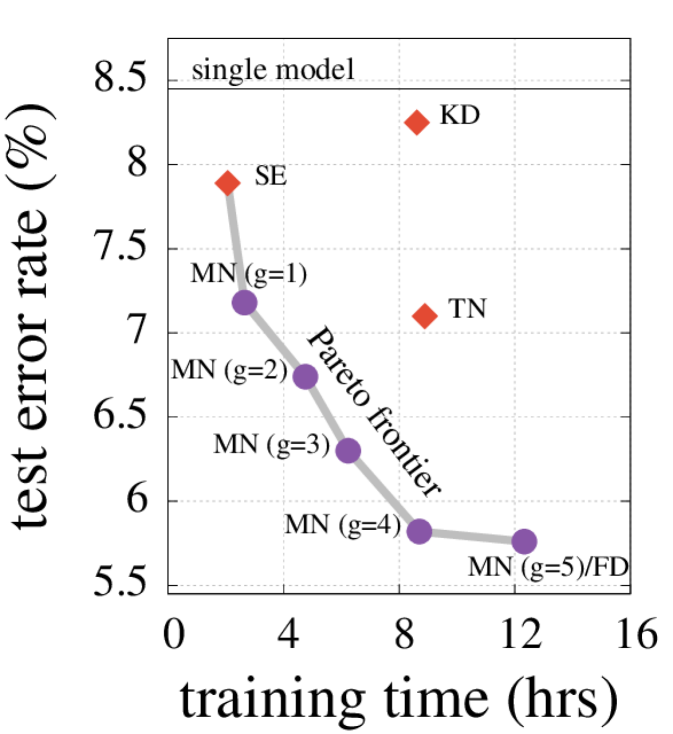
(a) V5 (C-10)

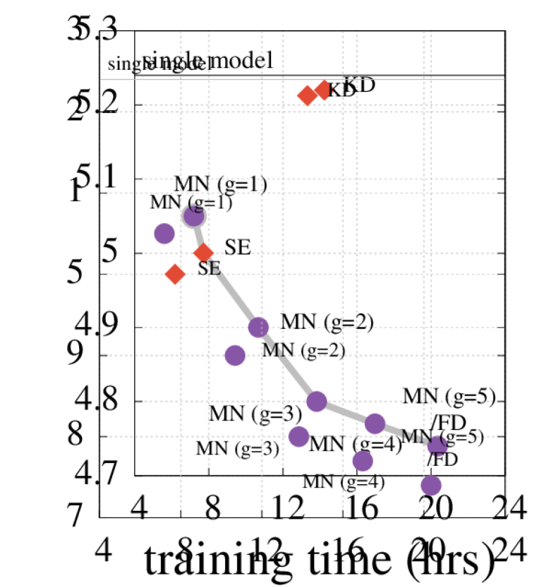
(b) D5 (C-10)

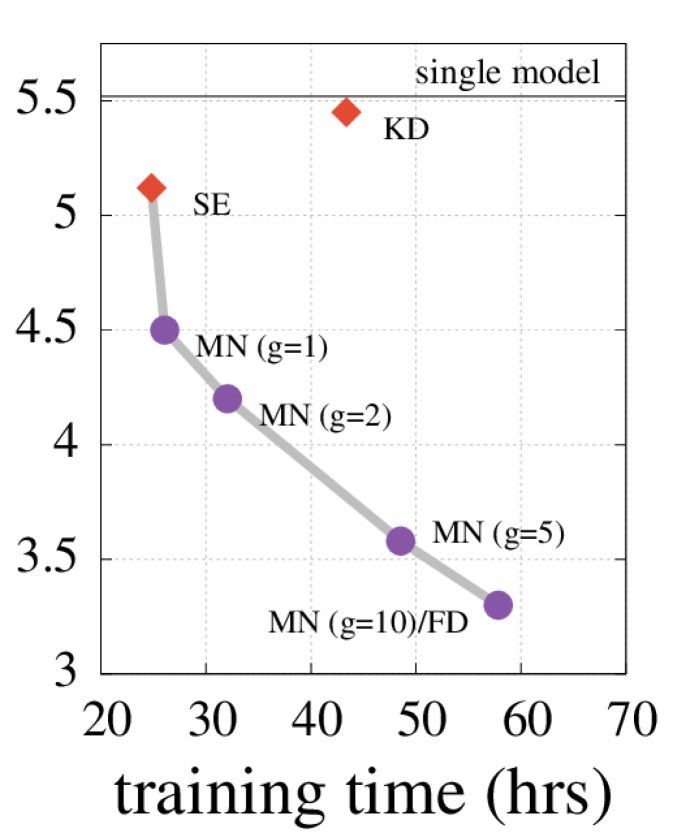
(c) R10 (C-10)

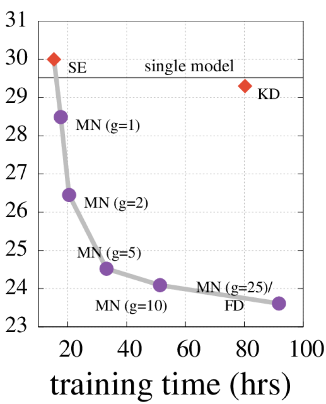
(d) V25 (C-100)

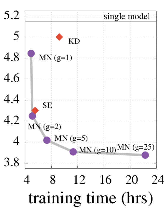
(e) V25 (SVHN)

Figure 4: MotherNets provide consistently better accuracy-training time tradeoff when compared with existing fast ensemble training approaches across various data sets, architectures, and ensemble sizes.

3 Experimental Analysis

We demonstrate that MotherNets enable a better training time-accuracy tradeoff than existing fast ensemble training approaches across multiple data sets and architectures. We also show that MotherNets make it more realistic to utilize large neural network ensembles.

Baselines. We compare against five state-of-the-art methods spanning both techniques that train all ensemble networks individually, i.e., Full Data (FD) and Bagging (BA), as well as approaches that generate ensembles by training a single network, i.e., Knowledge Distillation (KD), Snapshot Ensembles (SE), and TreeNets (TN).

Evaluation metrics. We capture both the training cost and the resulting accuracy of an ensemble. For the training cost, we report the wall clock time as well as the monetary cost for training on the cloud. For ensemble test accuracy, we report the test error rate under the widely used ensemble-averaging method Van der Laan et al. (2007); Guzman-Rivera et al. (2012; 2014); Lee et al. (2015b). Experiments with alternative inference methods (e.g., super learner and voting Ju et al. (2017)) showed that the method we use does not affect the overall results in terms of comparing the training algorithms.

Ensemble networks. We experiment with ensembles of various convolutional architectures such as VGGNets, ResNets, Wide ResNets, and DenseNets. Ensembles of these architectures have been extensively used to evaluate fast ensemble training approaches Lee et al. (2015a); Huang et al. (2017a). Each of these ensembles are composed of networks having diverse architectures as described in Table 2.

To provide a fair comparison with SE (where the snapshots have to be from the same network architecture), we create snapshots having comparable number of parameters to each of the ensembles described above. This comparable alternatives we used for SE are also summarized in Table 2.

For TN, we varied the number of shared layers and found that sharing the $3$ initial layers provides the best accuracy. This is similar to the optimal proportion of shared layers in the TreeNets paper Lee et al. (2015a). TN is not applicable to DenseNets or ResNets as it is designed only for networks without skip-connections Lee et al. (2015a). We omit comparison with TN for such ensembles.

Training setup. For all training approaches we use stochastic gradient descent with a mini-batch size of $256$ and batch-normalization. All weights are initialized by sampling from a standard normal distribution. Training data is randomly shuffled before every training epoch. The learning rate is set to $0.1$ with the exception of DenseNets. For DenseNets, we use a learning rate of $0.1$ to train MotherNets and $0.01$ to train hatched networks. This is inline with the learning rate decay used in the DenseNets paper Huang et al. (2017b). For FD, KD, TN, and MotherNets, we stop training if the training accuracy does not improve for 15 epochs. For SE we use the optimized training setup proposed in the original paper Huang et al. (2017a), starting with an initial learning rate of 0.2 and then training every snapshot for 60 epochs.

Data sets. We experiment with a diverse array of data sets: SVHN, CIFAR-10, and CIFAR-100 Krizhevsky (2009); Netzer et al. . The SVHN data set is composed of images of house numbers and has ten class labels. There are a total of $99$K images. We use $73$K for training and $26$K for testing. The CIFAR-10 and CIFAR-100 data sets have $10$ and $100$ class labels respectively corresponding to various images of everyday objects. There are a total of $60$K images – $50$K training and $10$K test images.

Hardware platform. All experiments are run on the same server with Nvidia Tesla V100 GPU.

3.1 Better training time-accuracy tradeoff

We first show how MotherNets strike an overall superior accuracy-training time tradeoff when compared to existing fast ensemble training approaches.

Figure 4 shows results across all our test data sets and ensemble networks. All graphs in Figure 4 depict the tradeoff between training time needed versus accuracy achieved. The core observation from Figure 4 is that across all datasets and networks, MotherNets help establish a new Pareto frontier of this tradeoff. The different versions of MotherNets shown in Figure 4 represent different numbers of clusters used ($g$). When $g$=1, we use a single MotherNet, optimizing for training time, while when $g$ becomes equal to the ensemble size, we optimize for accuracy (effectively this is equal to FD as every network is trained independently in its own cluster).

The horizontal line at the top of each graph indicates the accuracy of the best-performing single model in the ensemble trained from scratch. This serves as a benchmark and, in the vast majority of cases, all approaches do improve over a single model even when they have to sacrifice on accuracy to improve training time. MotherNets is consistently and significantly better than that benchmark.

Next we discuss each individual training approach and how it compares to MotherNets.

MotherNets vs. KD, TN, and BA. MotherNets (with $g$=1) is $2\times$ to $4.2\times$ faster than KD and results in up to $2$ percent better test accuracy. KD suffers in terms of accuracy because its ensemble networks are more closely tied to the base network as they are trained from the output of the same network. KD’s higher training cost is because distilling is expensive. Every network starts from scratch and is trained on the data set using a combination of empirical loss and the loss from the output of the teacher network. We observe that distilling a network still takes around $60$ to $70$ percent of the time required to train it using just the empirical loss.

To achieve comparable accuracy to MotherNets (with $g$=1), TN requires up to $3.8\times$ more training time on $V5$. In the same time budget, MotherNets can train with $g$=4 providing over one percent reduction in test error rate. The higher training time of TN is due to the fact that it combines several networks together to create a monolithic architecture with various branches. We observe that training this takes a significant time per epoch as well as requires more epochs to converge. Moreover, TN does not generalize to neural networks with skip-connections.

Figure 4 does not show results for BA because it is an outlier. BA takes on average 73 percent of the time FD needs to train but results in significantly higher test error rate than any of the baseline approaches including the single model. Compared to BA, MotherNets is on average 3.6 $\times$ faster and results in significantly better accuracy – up to 5.5 percent lower absolute test error rate. These observations are consistent with past studies that show how BA is ineffective when training deep neural networks as it reduces the number of unique data items seen by individual networks Lee et al. (2015a).

Overall, the low test error rate of MotherNets when compared to KD, TN, and BA stems from the fact that transferring the learned function from MotherNets to target ensemble networks provides a good starting point as well as introduces regularization for further training. This also allows hatched ensemble networks to converge significantly faster, resulting in overall lower training time.

Training time breakdown. To better understand where the time goes during the training process, Figure 6 provides the time breakdown per ensemble network. We show this for the D5 ensemble and compare MotherNets (with $g$=1) with individual training approaches FD, BA, and KD. While other approaches spend significant time training each network, MotherNets, can train these networks very quickly after having trained the core MotherNet (black part in the MotherNets stacked bar in Figure 6). We observe similar time breakdown across all ensembles in our experiments.

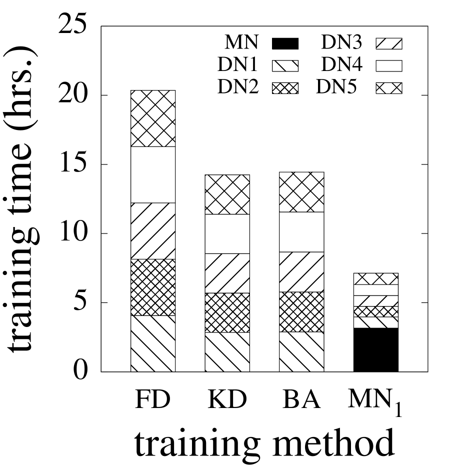
Figure 5: MotherNets train ensemble networks significantly faster after having trained the MotherNet (shown in black).

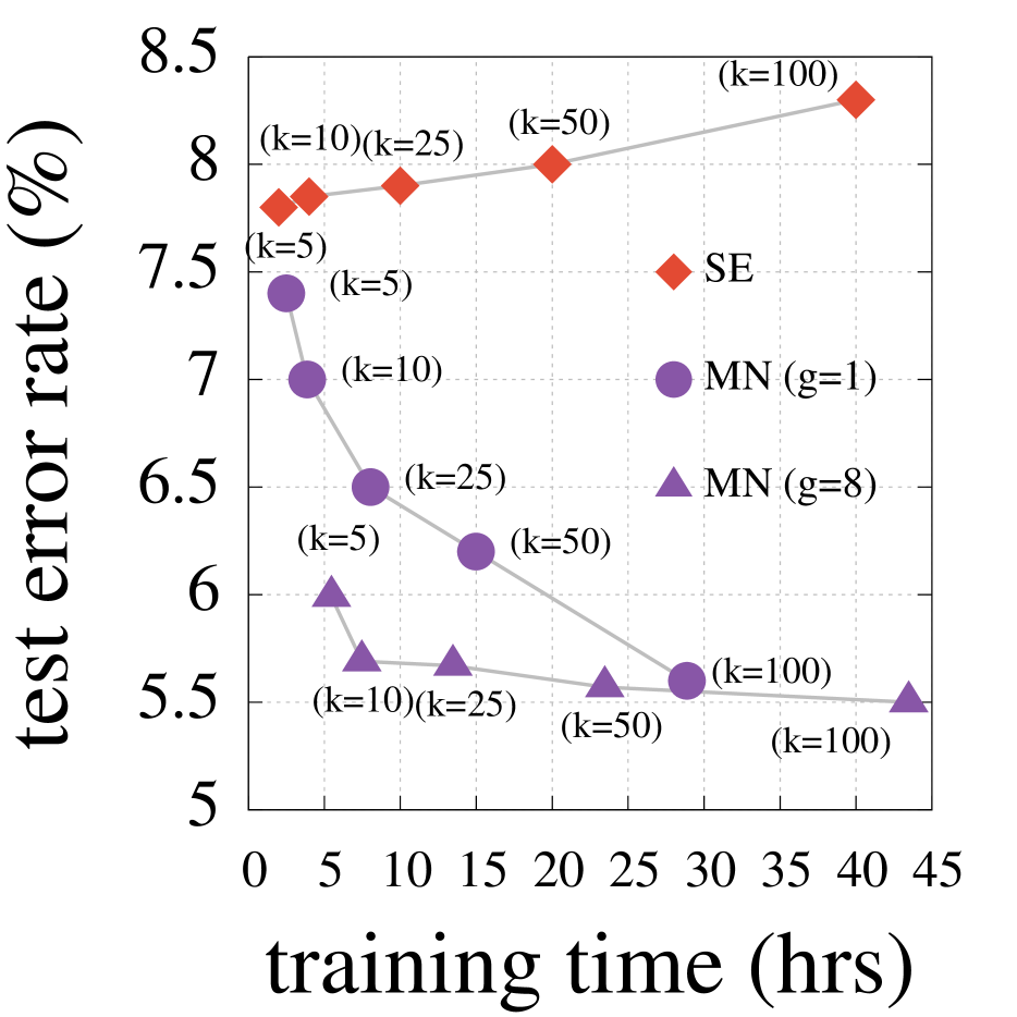
Figure 6: As the size of the ensemble grows, MotherNets scale better than SE both in terms of training time and accuracy achieved.

3.2 MotherNets vs. SE and scaling to large ensembles

Across all experiments in Figure 4, SE is the closest baseline to MotherNets. In effect, SE is part of the very same Pareto frontier defined by MotherNets in the accuracy-training cost tradeoff. That is, it represents one more valid point that can be useful depending on the desired balance. For example, in Figure 4(a) (for V5 CIFAR-10), SE sacrifices nearly one percent in test error rate compared to MotherNets (with $g$=1) for a small improvement in training cost. We observe similar trends in Figure 4(c) and 4(d)). In Figure 4(b), SE achieves a balance that is in between MotherNets with one and two clusters. However, when training V25 on SVHN (Figure 4(e)) SE is in fact outside the Pareto frontier as it is both slower and achieves worst accuracy.

Overall, MotherNets enables drastic improvements in either accuracy or training time compared to SE by being able to control and navigate the tradeoff between the two.

Table 3: MotherNets (with $g$=1) give better oracle test accuracy compared to Snapshot ensembles.

	V5 C10	D5 C10	R10 C10	V25 C100	V25 SVHN
MN	96.71	97.43	98.61	87.5	97.17
SE	96.03	96.91	97.11	86.9	97.3

Oracle accuracy. Also, Table 3 shows that MotherNets (with $g$=1) enable better oracle test accuracy when compared with SE across all our experiments. This is the accuracy if an oracle were to pick the prediction of the most accurate network in the ensemble per test element Guzman-Rivera et al. (2012; 2014); Lee et al. (2015b). Oracle accuracy is an upper bound for the accuracy that any ensemble inference technique could achieve. This metric is also used to evaluate the utility of ensembles when they are applied to solve Multiple Choice Learning (MCL) problems Guzman-Rivera et al. (2014); Lee et al. (2016); Brodie et al. (2018).

Scaling to very large ensembles. As we discussed before, large ensembles help improve accuracy and thus ideally we would like to scale neural network ensembles to large number of models as it happens for other ensembles such as random forests Oshiro et al. (2012); Bonab & Can (2016; 2017). Our previous results were for small to medium ensembles of 5, 10 or 25 networks. We now show that when it comes to larger ensembles, MotherNets dominate SE in both how accuracy and training time scale.

Figure 6 shows results as we increase the number of networks up to a hundred variants of VGGNets trained on CIFAR-10. For every point in Figure 6, $k$ indicates the number of networks. For MotherNets we plot results for the time-optimized version with $g$=1, as well as with $g$=8.

Figure 6 shows that as the size of the ensemble grows, MotherNets scale much better in terms of training time. Toward the end (for 100 networks), MotherNets train more than 10 hours faster (out of 40 total hours needed for SE). The training time of MotherNets grows at a much smaller rate because once the MotherNet has been trained, it takes $40$ percent less time to train a hatched network than the time it takes to train one snapshot.

In addition, Figure 6 shows that MotherNets does not only scale better in terms of training time, but also it scales better in terms of accuracy. As we add more networks to the ensemble, MotherNets keeps improving its error rate by nearly 2 percent while SE actually becomes worse by more than 0.5 percent. The declining accuracy of SE as the size of the ensemble increases has also been observed in the past, where by increasing the number of snapshots above six results in degradation in performance Huang et al. (2017a).

Finaly, Figure 6 shows that different cluster settings for MotherNets allow us to achieve different performance balances while still providing robust and predictable navigation of the tradeoff. In this case, with $g$=8 accuracy improves consistently across all points (compared to $g$=1) at the cost of extra training time.

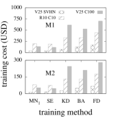
Figure 7: Training cost (USD)

3.3 Improving cloud training cost

One approach to speed up training of large ensembles is to utilize more than one machines. For example, we could train $k$ individual networks in parallel using $k$ machines. While this does save time, the holistic cost in terms of energy and resources spent is still linear to the ensemble size.

One proxy for capturing the holistic cost is to look at the amount of money one has to pay on the cloud for training a given ensemble. In our next experiment, we compare all approaches using this proxy. Figure 7 shows the cost (in USD) of training on four cloud instances across two cloud service providers: (i) M1 that maps to AWS P2.xlarge and Azure NC6, and (ii) M2 that maps to AWS P3.2xlarge and Azure NCv3. M1 is priced at USD $0.9$ per hour and M2 is priced at USD $3.06$ per hour for both cloud service providers Amazon (2019); Microsoft (2019).

Training time-optimized MotherNets provide significant reduction in training cost (up to $3\times$) as it can train a very large ensemble in a fraction of the training time compared to other approaches.

3.4 Diversity of model predictions

Next, we analyze how diversity of ensembles produced by MotherNets compares with SE and FD.

Ensembles and predictive diversity. Theoretical results suggest that ensembles of models perform better when the models’ predictions on a single example are less correlated. This is true under two assumptions: (i) models have equal correct classification probability and (ii) the ensemble uses majority vote for classification Krogh & Vedelsby (1994); Rosen (1996); Kuncheva & Whitaker (2003). Under ensemble averaging, no analytical proof that negative correlation reduces error rate exists, but lower correlation between models can be used to create a smaller upper bound on incorrect classification probability. More precise statements and their proofs are given in Appendix B.

Rapid ensemble training methods. For MotherNets, as well as for all other compared techniques for ensemble training, the training procedure binds the models together to decrease training time. This can have two negative effects compared to independent training of models:

1. by changing the model’s architecture or training pattern, the technique affects each model’s prediction quality (the model’s marginal prediction accuracy suffers)

2. by sharing layers (TN), attempted softmax values (KD), or training epochs (SE, MN), the training technique creates positive correlations between model errors.

We compare here the magnitude of these two effects forMotherNets and Snapshot Ensembles when compared to independent training of each model on CIFAR-10 using V5.

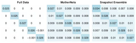
Figure 8: MotherNets (with $g$=1) train ensembles with lower model covariances compared to Snapshot Ensembles.

Individual model quality. For both SE and MN, the individual model accuracy drops, but the effect is more pronounced in SE than MN. The mean misclassification percentage of the individual models for V5 using FD, MN and SE are $8.1\%$, $8.4\%$ and $9.8\%$ respectively. The poor performance of SE in this area is due to its difficulty in consistently hitting performant local minima, either because it overfits to the training data when trained for a long time or because its early snapshots need to be far away from the final optimum to encourage diversity.

Model variance. Our goal in assessing variance is to see how the training procedure affects how models in the ensemble correlate with each other on each example. To do this, we train each of the five models in $V5$ five times under MN, SE, and FD. Letting $Y_{ij}$ be the softmax of the correct model on test example $j$ using model $i$, we then estimate $Var(Y_{ij})$ for each $i,j$ and $Cov(Y_{ij},Y_{i^{\prime}j})$ for each $i,i^{\prime},j$ with $i\neq i^{\prime}$ using the sample variance and covariance. To get a single number for a model, instead of one for each test example, we then average across all test examples, i.e. $Cov(Y_{i},Y_{i^{\prime}})=\frac{1}{n}\sum_{j=1}^{n}Cov(Y_{ij},Y_{i^{\prime}j})$. For total variance numbers for the ensemble, we perform the same procedure on $Y_{j}=\frac{1}{5}\sum_{i=1}^{5}Y_{ij}$.

Figure 8 shows the results. As expected, independent training between the models in FD makes their corresponding covariance 0 and provides the greatest overall variance reduction for the ensemble, with ensemble variance at $0.0051$. For both SE and MN, the covariance of separate models is non-zero at around $0.009$ per pair of models; however, it is also significantly less than the variance of a single model. As a result, both MN and SE provide significant variance reduction compared to a single model. Whereas a single model has variance around $0.026$, MN and SE provide ensemble variance of $0.0125$ and $0.0130$ respectively.

Takeaways. Since both SE and MN train nearly as fast as a single model, they provide variance reduction in prediction at very little training cost. Additionally, for MN, at the cost of higher training time, one can create more clusters and thus make the training of certain models independent of each other, zeroing out many of the covariance terms and reducing the overall ensemble variance. When compared to each other, MN with $g$=1 and SE have similar variance numbers, with MN slightly lower, but MotherNets has a substantial increase in individual model accuracy when compared to Snapshot Ensembles. As a result, its overall ensemble performs better.

Additional results. We demonstrate in Appendix C how MotherNets can improve inference time by $2\times$. In Appendix D, we show how the relative behavior of MotherNets remains the same when training using multiple GPUs. Finally, in Appendix E we provide experiments with Wide ResNets and demonstrate how MotherNets provide better accuracy-training time tradeoff when compared with Fast Geometric Ensembles.

4 Related Work

In this section, we briefly survey additional (but orthogonal) ensemble training techniques beyond Snapshot Ensembles, TreeNets, and Knowledge Distillation.

Parameter sharing. Various related techniques share parameters between different networks during ensemble training and, in doing so, improve training cost. One interpretation of techniques such as Dropout and Swapout is that, during training, they create several networks with shared weights within a single network. Then, they implicitly ensemble them during inference Wan et al. (2013); Srivastava et al. (2014); Huang et al. (2016); Singh et al. (2016); Huang et al. (2017a). Our approach, on the other hand, captures the structural similarity in an ensemble, where members have different and explicitly defined neural network architectures and trains it. Overall, this enables us to effectively combine well-known architectures together within an ensemble. Furthermore, implicit ensemble techniques (e.g., dropout and swapout) can be used as training optimizations to improve upon the accuracy of individual networks trained in MotherNets Srivastava et al. (2014); Singh et al. (2016).

Efficient deep network training. Various algorithmic techniques target fundamental bottlenecks in the training process Niu et al. (2011); Brown et al. (2016); Bottou et al. (2018). Others apply system-oriented techniques to reduce memory overhead and data movement De Sa & Feldman (2017); Jain et al. (2018). Recently, specialized hardware is being developed to improve performance, parallelism, and energy consumption of neural network training Prabhakar et al. (2016); De Sa & Feldman (2017); Jouppi et al. (2017). All techniques to improve upon training efficiency of individual neural networks are orthogonal to MotherNets and in fact directly compatible. This is because MotherNets does not make any changes to the core computational components of the training process. In our experiments, we do utilize some of the widely applied training optimizations such as batch-normalization and early-stopping. The advantage that MotherNets bring on top of these approaches is that we can further reduce the total number of epochs that are required to train an ensemble. This is because a set of MotherNets will train for the structural similarity present in the ensemble.

5 Conclusion

We present MotherNets which enable training of large and diverse neural network ensembles while being able to navigate a new Pareto frontier with respect to accuracy and training cost. The core intuition behind MotherNets is to reduce the number of epochs needed to train an ensemble by capturing the structural similarity present in the ensemble and training for it once.

6 Acknowledgments

We thank reviewers for their valuable feedback. We also thank Chang Xu for building the web-based demo and all DASlab members for their help. This work was partially funded by Tableau, Cisco, and the Harvard Data Science Institute.

Appendix

Algorithm A Constructing the MotherNet for fully-connected neural networks

Input: E: ensemble networks in one cluster;
Initialize: M: empty MotherNet;

// set input/output layer sizes M.input.num_param $\leftarrow$ E[0].input.num_param;
M.output.num_param $\leftarrow$ E[0].output.num_param;
M.num_layers $\leftarrow$ getShallowestNetwork(E).num_layers;

// set hidden layer sizes

for $i\leftarrow$ 0 …M.num_layers-1 do

       M.layers[i].num_param $\leftarrow$ getMin(E,i);

return M;
// Get the min. size layer at posn Function getMin(E,posn)

       min $\leftarrow$ E[0].layers[posn].num_param;
for $j\leftarrow$ 0 …len(E)-1 do

             if E[j].layers[posn].num_param $<$ min then

                   min $\leftarrow$ E[j].layers[posn].num_param

            

      return min;

A Algorithms for constructing MotherNets

We outline algorithms for constructing the MotherNet given a cluster of neural networks. We describe the algorithms for both fully-connected and convolutional neural networks.

Fully-Connected Neural Networks. Algorithm A describes how to construct the MotherNet for a cluster of fully-connected neural networks. We proceed layer-by-layer selecting the layer with the least number of parameters at every position.

Convolutional Neural Networks. Algorithm B provides a detailed strategy to construct the MotherNet for a cluster of convolutional neural networks. We proceed block-by-block, where each block is composed of multiple convolutional layers. The MotherNet has as many blocks as the network with the least number of blocks. Then, for every block, we proceed layer-by-layer and construct the MotherNet layer at every position as follows: First, we compute the least number of convolutional filters and convolutional filter sizes at that position across all ensemble networks. Let these be $F_{min}$ and $S_{min}$ respectively. Then, in MotherNet, we include a convolutional layer with $F_{min}$ filters of $S_{min}$ size at that position.

Algorithm B Constructing the MotherNet for convolutional neural networks block-by-block.

Input: E: ensemble of convolutional networks in one cluster;
Initialize: M: empty MotherNet; // set input/output layer sizes and number of blocks

M.input.num_param $\leftarrow$ E[0].input.num_param;
M.output.num_param $\leftarrow$ E[0].output.num_param;
M.num_blocks $\leftarrow$ getShallowestNetwork(E).num_blocks;

// set hidden layers block-by-block

for $k\leftarrow$ 0 …M.num_blocks-1 do

       M.block[k].num_hidden $\leftarrow$ getShallowestBlockAt(E,k).num_hidden; // select the shallowest block for $i\leftarrow$ 0 …M.block[k].num_hidden-1 do

             M.block[k].hidden[i]..num_filters, M.block[k].hidden[i]..filter_size $\leftarrow$ getMin(E,k,i)

      

return M;
// Get minimum number of filters and filter size at posn Function getMin(E,blk,posn)

       min_num_filters $\leftarrow$ E[0].block[blk].hidden[posn].num_filters;
min_filter_size $\leftarrow$ E[0].block[blk].hidden[posn].filter_size;
for $j\leftarrow$ 0 …len(E) do

             if E[j].block[blk].hidden[posn].num_filters $<$ min_num_filters then

                   min_num_filters $\leftarrow$ E[j].block[blk].hidden[posn].num_filters;

            if E[j].block[blk].hidden[posn].filter_size $<$ min_filter_size then

                   min_filter_size $\leftarrow$ E[j].block[blk].hidden[posn].filter_size;

            

      return min_num_filters, min_filter_size;

B Model Covariance and Ensemble Predictive Accuracy

We can analyze how model covariance effects ensemble performance by using Chebyshev’s Inequality to bound the chance that a model predicts an example incorrectly. By showing that lower covariance between models makes this bound on the probability smaller, we give an intuitive reason why ensembles with lower covariance between models perform better. The proof shows as well that the average model’s predictive accuracy is important; finally, no assumptions need to be made for the proof to hold. The individual models can be of different quality and have different chances of getting each example correct.

Given a fixed training dataset, let $Y_{i}$ be the softmax value of model $i$ in the ensemble for the correct class, and let $\hat{Y}=\frac{1}{m}\sum_{i=1}^{m}Y_{i}$ be the ensemble’s average softmax value on the correct class. Both are random variables with the randomness of $\hat{Y}$ and $Y_{i}$ coming through the randomness of neural network training. Under the mild assumption that $E[\hat{Y}]>\frac{1}{2}$, so that the a one vs. all softmax classifier would say on average that the correct class is more likely, than Chebyshev’s Inequality bounds the probability of incorrect prediction. Namely, the correct prediction is made with certainty if $\hat{Y}\geq\frac{1}{2}$ and so the probability of incorrect prediction is less than

$$P(|\hat{Y}-E[\hat{Y}]|\geq E[\hat{Y}]-\frac{1}{2})\leq\frac{Var(\hat{Y})}{(E[\hat{Y}]-\frac{1}{2})^{2}}$$

From the form of the equation, we immediately see that keeping the average model accuracy $E[Y_{i}]$ high is important, and that degradation in model quality can offset reductions in variance. Since the variance of $\hat{Y}$ decomposes into $\frac{1}{m^{2}}(\sum_{i=1}^{m}Var(Y_{i})+\sum_{i\neq i^{\prime}}Cov(Y_{i},Y_{i^{\prime}}))$, we see that low model covariance keeps the variance of the ensemble low, and that models which have which have high covariance with other models provides little benefit to the ensemble.

We explain how MotherNets improve the efficiency of ensemble inference.

Ensemble inference. Inference in an ensemble of neural networks proceeds as follows: First, the data item (e.g., an image or a feature vector) is passed through every network in the ensemble. These forward passes produce multiple predictions – one prediction for every network in the ensemble. The prediction of the ensemble is then computed by combining the individual predictions using some averaging or voting function. As the size of the ensemble grows, the inference cost in terms of memory and time required for inference increases linearly. This is because for every additional ensemble network, we need to maintain its parameters as well as do an additional forward pass on them.

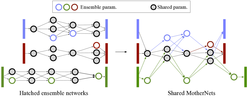
Figure A: To construct a shared-MotherNet, parameters originating from the MotherNet are combined together in the ensemble.

C Shared-MotherNets

Shared-MotherNets. We introduce shared-MotherNets to reduce inference time and memory requirement of ensembles trained through MotherNets. In shared-MotherNets, after the process of hatching (step 2 from §2), the parameters originating from the MotherNet are incrementally trained in a shared manner. This yields a neural network ensemble with a single copy of MotherNet parameters reducing both inference time and memory requirement.

Figure B: Shared MotherNets improve inference time by 2$\times$ for the V5 ensemble.

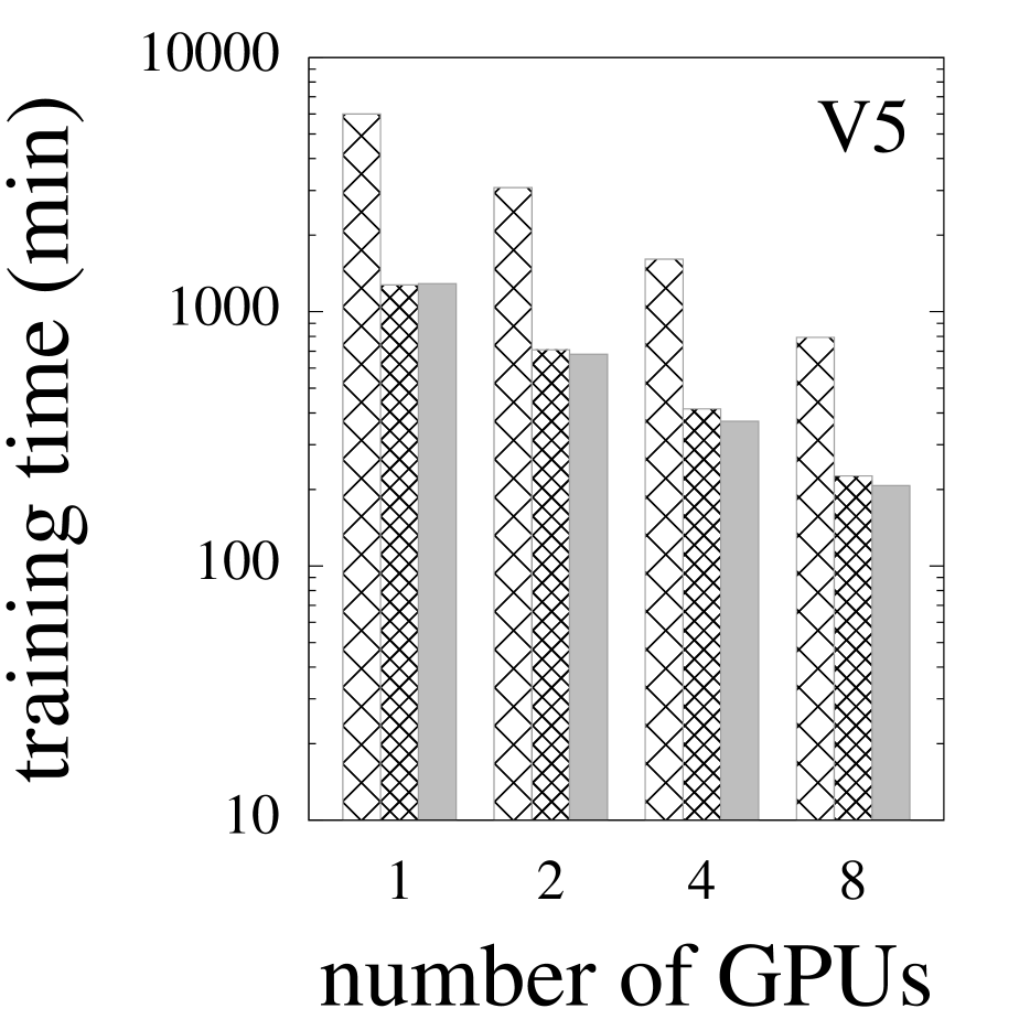
Figure C: MotherNets continue to improve training cost in parallel settings (V5).

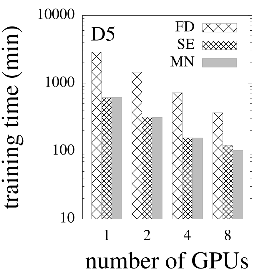
Figure D: MotherNets is able to utilize multiple GPUs effectively scaling better than SE.

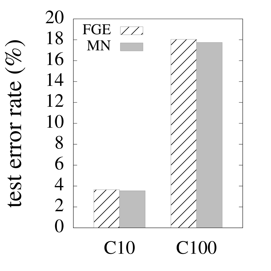
Figure E: MotherNets outperform FGE on Wide ResNet ensembles.

Constructing a shared-MotherNet. Given an ensemble $E$ of $K$ hatched networks (i.e., those networks that are obtained from a trained MotherNet), we construct a shared-MotherNet $S$ as follows: First, $S$ is initialized with $K$ input and output layers, one for every hatched network. This allows $S$ to produce as many as $K$ predictions. Then, every hidden layer of $S$ is constructed one-by-one going from the input to the output layer and consolidating all neurons across all of $E$ that originate from the MotherNet. To consolidate a MotherNet neuron at layer $l_{i}$, we first reduce the $k$ copies of that neuron (across all $K$ networks in H) to a single copy. All inputs to the neuron that may originate from various other neurons in the layer $l_{i-1}$ across different hatched networks are added together. The output of this consolidated neuron is then forwarded to all neurons in the next layer $l_{i+1}$ (across all hatched networks) which were connected to the consolidated neuron.

Figure A shows an example of how this process works for a simple ensemble of three hatched networks. The filled circles represent neurons originating from the MotherNet and the colored circles represent neurons from ensemble networks. To construct the shared-MotherNet (shown on the right), we go layer-by-layer consolidating MotherNet neurons.

The shared-MotherNet is then trained incrementally. This proceeds similarly to step 3 from §2, however, now through the shared-MotherNet, the neurons originating from the MotherNet are trained jointly. This results in an ensemble that has $K$ outputs, but some parameters between the networks are shared instead of being completely independent. This reduces the overall number of parameters, improving both the speed and the memory requirement of inference.

Memory reduction. Assume an ensemble $E=\{N_{0},N_{1},\dots N_{K-1}\}$ of $K$ neural networks (where $N_{i}$ denotes a neural network architecture in the ensemble with $|N_{i}|$ number of parameters) and its MotherNet $M$. The number of parameters in the ensemble is reduced by a factor of $\chi$ given by:

$$\chi=1-\frac{k|M|}{\sum_{i=0}^{K-1}|N_{i}|}$$

Results. Figure E shows how shared-MotherNets improves inference time for an ensemble of 5 variants of VGGNet as described in Table 1. This ensemble is trained on the CIFAR-10 data set. We report both overall ensemble test error rate and the inference time per image. We see an improvement of $2\times$ with negligible loss in accuracy. This improvement is because shared-MotherNets has a reduced number of parameters requiring less computation during inference time. This improvement scales with the ensemble size.

D Parallel training

Deep learning pipelines rely on clusters of multiple GPUs to train computationally-intensive neural networks. MotherNets continue to improve training time in such cases when an ensemble is trained on more than one GPUs. We show this experimentally.

To train an ensemble of multiple networks, we queue all networks that are ready to be trained and assign them to available GPUs in the following fashion: If the number of ready networks is greater than free GPUs, then we assign a separate network to every GPU. If the number of ensemble networks available to be trained are less than the number of idle GPUs, then we assign one network to multiple GPUs dividing idle GPUs equally between networks. In such cases, we adopt data parallelism to train a network across multiple machines Dean et al. (2012).

We train on a cluster of 8 Nvidia K80 GPUs and vary the number of available GPUs from 1 to 8. The training hyperparameters are the same as described in Section 3. Figure E and Figure E show the time to train the V5 and D5 ensembles respectively across FD, SE, and MotherNets. We observe that compared to Snapshot Ensembles, MotherNets (g=1) scale better as we increase the number of GPUs. The reason for this is that after the MotherNet has been trained, the rest of the ensemble networks are all ready to be trained. They can then be trained in a way that minimizes communication overhead by assigning them to as distinct set of GPUs as possible. Snapshot Ensembles, on the other hand, are generated one after the other. In a parallel setting this boils down to training a single network across multiple GPUs, which incurs communication overhead that increases as the number of GPUs increases Keuper & Preundt (2016).

E Improving over Fast Geometric Ensembles

Now we compare against Fast Geometric Ensembles (FGE), a technique closely related to Snapshot Ensembles (SE) Huang et al. (2017a); Garipov et al. (2018). FGE also trains a single neural network architecture and saves the network’s parameters at various points of its training trajectory. In particular, FGE uses a cyclical geometric learning rate schedule to explore various regions in a neural network’s loss surface that have a low test error Garipov et al. (2018). As the learning rate reaches its lowest value in a cycle, FGE saves ‘snapshots’ of the network parameters. These snapshots are then used in an ensemble.

We compare MotherNets to FGE using an ensemble of Wide Residual Networks trained on CIFAR-10 and CIFAR-100 Zagoruyko & Komodakis (2016). Our experiment consists of an ensemble with six WRN-28-10. For MotherNets, we use six variants of this architecture having different number of filters and filter widths. For FGE all networks in the ensemble are the same as is required by the approach. For a fair comparison, the number of parameters are kept identical between the two approaches. We use the same training hyperparameters as discussed in the FGE paper and train for a full training budget of 200 epochs. MotherNets is also allocated the same training budget. The MotherNet is trained for a $140$ epochs and every ensemble network is trained for $10$ epochs after hatching. The experimental hardware is the same as outlined in Section 3. Figure E shows that for identical training budget MotherNets is more accurate than FGE across both data sets.

References

- Agrafiotis et al. (2002) Agrafiotis, D. K., Cedeno, W., and Lobanov, V. S. On the use of neural network ensembles in qsar and qspr. Journal of chemical information and computer sciences, 42(4), 2002.
- Amazon (2019) Amazon. Aws pricing. https://aws.amazon.com/pricing/, 2019. (Accessed on 05/16/2019).
- Arumugam et al. (2010) Arumugam, S., Dobra, A., Jermaine, C. M., Pansare, N., and Perez, L. The DataPath System: A Data-centric Analytic Processing Engine for Large Data Warehouses. In Proceedings of the ACM SIGMOD International Conference on Management of Data, pp. 519–530, 2010. URL http://dl.acm.org/citation.cfm?id=1807167.1807224.
- Bonab & Can (2016) Bonab, H. R. and Can, F. A theoretical framework on the ideal number of classifiers for online ensembles in data streams. In Proceedings of the 25th ACM International on Conference on Information and Knowledge Management, 2016.
- Bonab & Can (2017) Bonab, H. R. and Can, F. Less is more: A comprehensive framework for the number of components of ensemble classifiers. IEEE Transactions on Neural Networks and Learning Systems, 2017.
- Bottou et al. (2018) Bottou, L., Curtis, F. E., and Nocedal, J. Optimization methods for large-scale machine learning. SIAM Review, 60(2), 2018.
- Brodie et al. (2018) Brodie, M., Tensmeyer, C., Ackerman, W., and Martinez, T. Alpha model domination in multiple choice learning. In IEEE International Conference on Machine Learning and Applications (ICMLA), 2018.
- Brown et al. (2016) Brown, K. J., Lee, H., Rompf, T., Sujeeth, A. K., Sa, C. D., Aberger, C. R., and Olukotun, K. Have abstraction and eat performance, too: Optimized heterogeneous computing with parallel patterns. In Proceedings of the International Symposium on Code Generation and Optimization, 2016.
- Cai et al. (2018) Cai, H., Chen, T., Zhang, W., Yu, Y., and Wang, J. Efficient architecture search by network transformation. In AAAI Conference on Artificial Intelligence, 2018.
- Candea et al. (2011) Candea, G., Polyzotis, N., and Vingralek, R. Predictable Performance and High Query Concurrency for Data Analytics. The VLDB Journal, 20(2):227–248, 2011. URL http://dl.acm.org/citation.cfm?id=1969331.1969355.
- Chen et al. (2016) Chen, T., Goodfellow, I. J., and Shlens, J. Net2net: Accelerating learning via knowledge transfer. In International Conference on Learning Representations (ICLR), San Juan, Puerto Rico, May 2-4, 2016, Conference Track Proceedings, 2016.
- De Sa & Feldman (2017) De Sa, C. and Feldman, M. Understanding and optimizing asynchronous low-precision stochastic gradient descent. In Annual International Symposium on Computer Architecture (ISCA), 2017.
- Dean et al. (2012) Dean, J., Corrado, G., Monga, R., Chen, K., Devin, M., Mao, M., Senior, A., Tucker, P., Yang, K., Le, Q. V., et al. Large scale distributed deep networks. In Advances in Neural Information Processing Systems, 2012.
- Dietterich (2000) Dietterich, T. G. Ensemble methods in machine learning. In International Workshop on Multiple Classifier Systems, 2000.
- Drucker et al. (1993) Drucker, H., Schapire, R., and Simard, P. Improving performance in neural networks using a boosting algorithm. In Advances in Neural Information Processing Systems, 1993.
- Garipov et al. (2018) Garipov, T., Izmailov, P., Podoprikhin, D., Vetrov, D. P., and Wilson, A. G. Loss surfaces, mode connectivity, and fast ensembling of dnns. In Advances in Neural Information Processing Systems, 2018.
- Giannikis et al. (2012) Giannikis, G., Alonso, G., and Kossmann, D. SharedDB: Killing One Thousand Queries with One Stone. Proceedings of the VLDB Endowment, 5(6):526–537, 2012. URL http://dl.acm.org/citation.cfm?id=2168651.2168654.
- Giannikis et al. (2014) Giannikis, G., Makreshanski, D., Alonso, G., and Kossmann, D. Shared Workload Optimization. Proceedings of the VLDB Endowment, 7(6):429–440, 2014. URL http://www.vldb.org/pvldb/vol7/p429-giannikis.pdf.
- Goodfellow et al. (2016) Goodfellow, I., Bengio, Y., and Courville, A. Deep Learning. MIT Press, 2016.
- Granitto et al. (2005) Granitto, P. M., Verdes, P. F., and Ceccatto, H. A. Neural network ensembles: Evaluation of aggregation algorithms. Artificial Intelligence, 163(2), 2005.
- Gulshan et al. (2016) Gulshan, V., Peng, L., Coram, M., Stumpe, M. C., Wu, D., Narayanaswamy, A., Venugopalan, S., Widner, K., Madams, T., Cuadros, J., et al. Development and validation of a deep learning algorithm for detection of diabetic retinopathy in retinal fundus photographs. Jama, 316(22), 2016.
- Gupta et al. (2016) Gupta, S., Zhang, W., and Wang, F. Model accuracy and runtime tradeoff in distributed deep learning: A systematic study. In IEEE International Conference on Data Mining (ICDM), 2016.
- Guzman-Rivera et al. (2012) Guzman-Rivera, A., Batra, D., and Kohli, P. Multiple choice learning: Learning to produce multiple structured outputs. In Advances in Neural Information Processing Systems, 2012.
- Guzman-Rivera et al. (2014) Guzman-Rivera, A., Kohli, P., Batra, D., and Rutenbar, R. Efficiently enforcing diversity in multi-output structured prediction. In Artificial Intelligence and Statistics, 2014.
- Harizopoulos et al. (2005) Harizopoulos, S., Shkapenyuk, V., and Ailamaki, A. QPipe: A Simultaneously Pipelined Relational Query Engine. In Proceedings of the ACM SIGMOD International Conference on Management of Data, pp. 383–394, 2005. URL http://dl.acm.org/citation.cfm?id=1066157.1066201.
- He et al. (2016) He, K., Zhang, X., Ren, S., and Sun, J. Deep residual learning for image recognition. In IEEE Conference on Computer Vision and Pattern Recognition (CVPR), 2016.
- Hinton et al. (2015) Hinton, G., Vinyals, O., and Dean, J. Distilling the knowledge in a neural network. In NIPS Deep Learning and Representation Learning Workshop, 2015.
- Huang et al. (2016) Huang, G., Sun, Y., Liu, Z., Sedra, D., and Weinberger, K. Q. Deep networks with stochastic depth. In European Conference on Computer Vision, 2016.
- Huang et al. (2017a) Huang, G., Li, Y., Pleiss, G., Liu, Z., Hopcroft, J. E., and Weinberger, K. Q. Snapshot ensembles: Train 1, get m for free. 5th International Conference on Learning Representations (ICLR), 2017a.
- Huang et al. (2017b) Huang, G., Liu, Z., van der Maaten, L., and Weinberger, K. Q. Densely connected convolutional networks. In IEEE Conference on Computer Vision and Pattern Recognition, (CVPR), 2017b.
- Huggins et al. (2016) Huggins, J., Campbell, T., and Broderick, T. Coresets for scalable bayesian logistic regression. In Advances in Neural Information Processing Systems, 2016.
- Iandola et al. (2016) Iandola, F. N., Moskewicz, M. W., Ashraf, K., and Keutzer, K. Firecaffe: Near-linear acceleration of deep neural network training on compute clusters. In IEEE Conference on Computer Vision and Pattern Recognition, 2016.
- Jain et al. (2018) Jain, A., Phanishayee, A., Mars, J., Tang, L., and Pekhimenko, G. Gist: Efficient data encoding for deep neural network training. In IEEE Annual International Symposium on Computer Architecture, 2018.
- Jouppi et al. (2017) Jouppi, N. P. et al. In-datacenter performance analysis of a tensor processing unit. In Annual International Symposium on Computer Architecture (ISCA), 2017.
- Ju et al. (2017) Ju, C., Bibaut, A., and van der Laan, M. J. The relative performance of ensemble methods with deep convolutional neural networks for image classification. CoRR, abs/1704.01664, 2017.
- Kester et al. (2017) Kester, M. S., Athanassoulis, M., and Idreos, S. Access Path Selection in Main-Memory Optimized Data Systems: Should I Scan or Should I Probe? In Proceedings of the ACM SIGMOD International Conference on Management of Data, pp. 715–730, 2017. ISBN 9781450341974. doi: 10.1145/3035918.3064049. URL http://dl.acm.org/citation.cfm?doid=3035918.3064049.
- Keuper & Preundt (2016) Keuper, J. and Preundt, F.-J. Distributed training of deep neural networks: Theoretical and practical limits of parallel scalability. In 2016 2nd Workshop on Machine Learning in HPC Environments (MLHPC), pp. 19–26. IEEE, 2016.
- Krizhevsky (2009) Krizhevsky, A. Learning multiple layers of features from tiny images. 2009.
- Krogh & Vedelsby (1994) Krogh, A. and Vedelsby, J. Neural network ensembles, cross validation and active learning. In International Conference on Neural Information Processing Systems, 1994.
- Kuncheva & Whitaker (2003) Kuncheva, L. I. and Whitaker, C. J. Measures of diversity in classifier ensembles and their relationship with the ensemble accuracy. Machine Learning, 51(2), 2003.
- Lee et al. (2015a) Lee, S., Purushwalkam, S., Cogswell, M., Crandall, D. J., and Batra, D. Why M heads are better than one: Training a diverse ensemble of deep networks. CoRR, abs/1511.06314, 2015a.
- Lee et al. (2015b) Lee, S., Purushwalkam, S., Cogswell, M., Crandall, D. J., and Batra, D. Why M heads are better than one: Training a diverse ensemble of deep networks. CoRR, abs/1511.06314, 2015b.
- Lee et al. (2016) Lee, S., Prakash, S. P. S., Cogswell, M., Ranjan, V., Crandall, D., and Batra, D. Stochastic multiple choice learning for training diverse deep ensembles. In Advances in Neural Information Processing Systems, 2016.
- Levenshtein (1966) Levenshtein, V. I. Binary codes capable of correcting deletions, insertions, and reversals. 1966.
- Li & Hoiem (2017) Li, Z. and Hoiem, D. Learning without forgetting. IEEE Transactions on Pattern Analysis and Machine Intelligence, 2017.
- MacQueen (1967) MacQueen, J. Some methods for classification and analysis of multivariate observations. In Berkeley Symposium on Mathematical Statistics and Probability, 1967.
- Microsoft (2019) Microsoft. Pricing - windows virtual machines | microsoft azure. https://azure.microsoft.com/en-us/pricing/details/virtual-machines/windows/, 2019. (Accessed on 05/16/2019).
- Moghimi & Vasconcelos (2016) Moghimi, M. and Vasconcelos, N. Boosted convolutional neural networks. In Proceedings of the British Machine Vision Conference, 2016.
- (49) Netzer, Y., Wang, T., Coates, A., Bissacco, A., Wu, B., and Ng, A. Y. Reading digits in natural images with unsupervised feature learning.
- Niu et al. (2011) Niu, F., Recht, B., Ré, C., and Wright, S. J. Hogwild!: A lock-free approach to parallelizing stochastic gradient descent. In Advances in Neural Information Processing Systems, 2011.
- Oshiro et al. (2012) Oshiro, T. M., Perez, P. S., and Baranauskas, J. A. How many trees in a random forest? In International Workshop on Machine Learning and Data Mining in Pattern Recognition. Springer, 2012.
- Prabhakar et al. (2016) Prabhakar, R., Koeplinger, D., Brown, K. J., Lee, H., Sa, C. D., Kozyrakis, C., and Olukotun, K. Generating configurable hardware from parallel patterns. In Proceedings of the Twenty-First International Conference on Architectural Support for Programming Languages and Operating Systems, ASPLOS ’16, Atlanta, GA, USA, April 2-6, 2016, pp. 651–665, 2016. doi: 10.1145/2872362.2872415. URL http://doi.acm.org/10.1145/2872362.2872415.
- Psaroudakis et al. (2013) Psaroudakis, I., Athanassoulis, M., and Ailamaki, A. Sharing Data and Work Across Concurrent Analytical Queries. Proceedings of the VLDB Endowment, 6(9):637–648, 2013. URL http://dl.acm.org/citation.cfm?id=2536360.2536364.
- Qiao et al. (2008) Qiao, L., Raman, V., Reiss, F., Haas, P. J., and Lohman, G. M. Main-memory Scan Sharing for Multi-core CPUs. Proceedings of the VLDB Endowment, 1(1):610–621, 2008. URL http://dl.acm.org/citation.cfm?id=1453856.1453924.
- Rosen (1996) Rosen, B. E. Ensemble learning using decorrelated neural networks. Connection Science, 1996.
- Russakovsky et al. (2015) Russakovsky, O., Deng, J., Su, H., Krause, J., Satheesh, S., Ma, S., Huang, Z., Karpathy, A., Khosla, A., Bernstein, M., et al. Imagenet large scale visual recognition challenge. International Journal of Computer Vision, 115(3), 2015.
- Shazeer et al. (2017) Shazeer, N., Mirhoseini, A., Maziarz, K., Davis, A., Le, Q., Hinton, G., and Dean, J. Outrageously large neural networks: The sparsely-gated mixture-of-experts layer. International Conference on Learning Representations (ICLR), 2017.
- Simonyan & Zisserman (2015) Simonyan, K. and Zisserman, A. Very deep convolutional networks for large-scale image recognition. In International Conference on Learning Representations (ICLR), 2015.
- Singh et al. (2016) Singh, S., Hoiem, D., and Forsyth, D. Swapout: Learning an ensemble of deep architectures. In Advances in Neural Information Processing Systems, 2016.
- Srivastava et al. (2014) Srivastava, N., Hinton, G., Krizhevsky, A., Sutskever, I., and Salakhutdinov, R. Dropout: A simple way to prevent neural networks from overfitting. The Journal of Machine Learning Research, 15(1), 2014.
- Szegedy et al. (2015) Szegedy, C., Liu, W., Jia, Y., Sermanet, P., Reed, S., Anguelov, D., Erhan, D., Vanhoucke, V., and Rabinovich, A. Going deeper with convolutions. In Computer Vision and Pattern Recognition (CVPR), 2015.
- Van der Laan et al. (2007) Van der Laan, M. J., Polley, E. C., and Hubbard, A. E. Super learner. Statistical applications in genetics and molecular biology, 6(1), 2007.
- Wan et al. (2013) Wan, L., Zeiler, M., Zhang, S., Le Cun, Y., and Fergus, R. Regularization of neural networks using dropconnect. In International Conference on Machine Learning, 2013.
- Wei et al. (2016) Wei, T., Wang, C., Rui, Y., and Chen, C. W. Network morphism. In International Conference on Machine Learning, 2016.
- Wei et al. (2017) Wei, T., Wang, C., and Chen, C. W. Modularized morphing of neural networks. CoRR, abs/1701.03281, 2017.
- Xu et al. (2014) Xu, L., Ren, J. S., Liu, C., and Jia, J. Deep convolutional neural network for image deconvolution. In Advances in Neural Information Processing Systems, 2014.
- Ye & Guo (2017) Ye, M. and Guo, Y. Self-training ensemble networks for zero-shot image recognition. Knowl.-Based Syst., 123:41–60, 2017.
- Zagoruyko & Komodakis (2016) Zagoruyko, S. and Komodakis, N. Wide residual networks. Proceedings of the British Machine Vision Conference, 2016.
- Zukowski et al. (2007) Zukowski, M., Héman, S., Nes, N. J., and Boncz, P. A. Cooperative Scans: Dynamic Bandwidth Sharing in a DBMS. In Proceedings of the International Conference on Very Large Data Bases (VLDB), pp. 723–734, 2007. URL http://dl.acm.org/citation.cfm?id=1325851.1325934.