A Singular Integral Measure for
$C^{1\mathord{}\mathchar 44\relax 1}$ and $C^{1}$ Boundaries

Abstract

The art of analysis involves the subtle combination of approximation, inequalities, and geometric intuition as well as being able to work at different scales. With this subtlety in mind, we present this paper in a manner designed for wide accessibility for both advanced undergraduate students and graduate students. The main results include a singular integral for measuring the level sets of a $C^{1\mathord{}\mathchar 44\relax 1}$ function mapping from $\mathbb{R}^{n}$ to $\mathbb{R}$, that is, one whose derivative is Lipschitz continuous. We extend this to measure embedded submanifolds in $\mathbb{R}^{2}$ that are merely $C^{1}$ using the distance function and provide an example showing that the measure does not hold for general rectifiable boundaries.

1 Introduction

Often times it happens that creative exploration leads to uncharted territory in mathematics. That is indeed the case in the development of the singular integral boundary measure for hypersurfaces in $\mathbb{R}^{n}$, presented below. To highlight this process, we shall first explore the simple analysis problem that led to our discovery of this integral and then present our singular integral that measures the $(n-1)$-dimensional Hausdorff measure $\mathcal{H}^{n-1}$ of level sets of $C^{1\mathord{}\mathchar 44\relax 1}$ functions, that is, those whose derivative is Lipschitz continuous.

Continuing the process of exploration and generalization, we present the same singular integral as a $C^{1}$-boundary measure using the distance function in $\mathbb{R}^{2}$. The arguments here are markedly different from the $C^{1\mathord{}\mathchar 44\relax 1}$ case and follow a “by-construction,” barehanded approach due to the fact that in this case, we may have $\epsilon$-neighborhoods of the boundary in which the normals intersect no matter how small $\epsilon$ is (i.e. we no longer have positive reach; see Definition 3.2), so we cannot use the Area Formula (see Theorem 3.2).

2 A Simple Analysis Problem

Consider the following simple analysis problem:

Problem 2.1.

For $f(x):\mathbb{R}\rightarrow\mathbb{R}$, suppose that $f(x)$ is differentiable, $f(0)=0$, and $\exists\lambda>0$ such that $\forall x\in\mathbb{R}$

$$\left|f^{\prime}(x)\right|\leq\lambda|f(x)|.$$ (1)

Prove that $f(x)=0$ everywhere.

Solution 1: ODE’s.

Take the families of curves in $\mathbb{R}^{2}$ $g_{C}=Ce^{2\lambda x}$ and $h_{C}=Ce^{-2\lambda x}$ as all the solutions to the differential equations $g^{\prime}=2\lambda g$ and $h^{\prime}=-2\lambda h$, respectively. Cleary $f(x)$ cannot simply be one of these curves since none of them are ever 0. Note that the 2 is included here so that any solution $f(x)$ that satisfies (1) that intersects one of these curves must cross it. Indeed, without loss of generality, suppose for $g_{C}$ there exists an $x_{0}$ such that for all $x>x_{0}$, $f(x)=C_{0}e^{2\lambda x}.$ Then we find that

$$\frac{2\lambda C_{0}e^{2\lambda x}}{C_{0}e^{2\lambda x}}\leq\lambda\Rightarrow 2\leq 1\mathord{}\mathchar 44\relax$$

a contradiction. A similar argument holds for $h_{C}$.

Now, for $g_{C}$, $f(x)$ can only cross from above to below as $x$ increases. If not, then $f^{\prime}(x)>C2\lambda e^{2\lambda x}=2\lambda f\Rightarrow\frac{f^{\prime}}{f}>2\lambda\mathord{}\mathchar 44\relax$ also a contradiction. Similarly, $f(x)$ can only cross $h_{C}$ from below to above as $x$ increases.

Now, suppose $f(x^{*})>0$ for some $x^{*}$ (for $f(x^{*})<0$, then $-f(x)$ satisfies (1) and is positive at $x^{*}$). Pick the corresponding $C^{+*}=f(x^{*})/e^{2\lambda x^{*}}$ for $g_{C^{+*}}$ and $C^{-*}=f(x^{*})/e^{-2\lambda x^{*}}$ for $h_{C^{-*}}$. These curves serve as “fences” ($g_{C^{+*}}$ for $x<x*$ and $h_{C^{-*}}$ for $x>x*$) that $f$ cannot cross so that $f\neq 0.$ Thus we have a contradiction which implies that $f(x)\equiv 0$ everywhere (see Figures 1, 2, and 3).

∎

Figure 1: The case where $f(x^{*})>0$ and $g_{C^{+*}}$ acts as a “fence” for $f(x)$ when $x<x*$, bounding it away from 0.

Figure 2: The case where $f(x^{*})>0$ and $h_{C^{-*}}$ acts as a “fence” for $f(x)$ when $x>x*$, bounding it away from 0.

Figure 3: The two combined cases from above.

Solution 2: Mean Value Theorem.

Suppose $f(x_{0})=0$. We prove $f(x)=0$ on $I=[x_{0}-\frac{1}{2\lambda}\mathchar 44\relax x_{0}+\frac{1}{2\lambda}]$. Cleary then we can pick the endpoints of this interval to extend our interval where $f(x)$ is 0. Continuing this process thus this implies that $f(x)$ is 0 everywhere.

Let $x\in I$. By the Mean Value Theorem,

$$|f(x)-f(x_{0})|\leq|f^{\prime}(y_{1})||x-x_{0}|\leq|f^{\prime}(y_{1})|\frac{1}{2\lambda}\mathord{}\mathchar 44\relax$$

for some $y_{1}\in I$. By (1), we have

$$|f(x)|=|f(x)-0|\leq|f^{\prime}(y_{1})|\frac{1}{2\lambda}\leq\frac{1}{2}f(y_{1}).$$

Similarly, $|f(y_{1})|\leq\frac{1}{2}f(y_{2})$ for some $y_{2}\in I$. Thus $|f(x)|\leq\frac{1}{2^{2}}f(y_{2})$. Continuing this process, we obtain

$$|f(x)|\leq\frac{1}{2^{n}}f(y_{n})$$ (2)

for some $y_{n}\in I\mathchar 44\relax n\in\mathbb{N}$.

From the Extreme Value Theorem, $f(x)$ continuous $\Rightarrow f(x)<M\text{ for all }x\in I$. Using this with (2), we get

$$|f(x)|\leq\frac{M}{2^{n}}\text{ for all }n\in\mathbb{N}.$$

Sending $n\rightarrow\infty$ gives $f(x)\equiv 0$.

∎

Solution 3: A Barehanded ODE Approach.

We shall construct “fences” similar to the first solution above. If $f(x)>0\ \forall x\in[x_{0}\mathord{}\mathchar 44\relax x_{1}]\subset E\subset\mathbb{R}$, then

$$\left|f^{\prime}(x)\right|\leq\lambda|f(x)|\ \Leftrightarrow\ -\lambda\leq\frac{f^{\prime}(x)}{f(x)}\leq\lambda.$$

Integrating both sides of this over the interval $[x_{0}\mathord{}\mathchar 44\relax x_{1}]$ gives

$$-\lambda(x_{1}-x_{0})\leq\ln\left(\frac{f(x_{1})}{f(x_{0})}\right)\leq\lambda(x_{1}-x_{0}).$$

But this is equivalent to

$$e^{-\lambda(x_{1}-x_{0})}\leq\frac{f(x_{1})}{f(x_{0})}\leq e^{\lambda(x_{1}-x_{0})}.$$ (3)

Now, let $f(x^{*})>0$. Define

$$l=\inf\{w|f(x)>0\text{ for all }w<x<x^{*}\}$$

and

$$u=\sup\{w|f(x)>0\text{ for all }x^{*}<x<w\}.$$

We see that $l\neq-\infty\Rightarrow f(l)=0$ and $u\neq\infty\Rightarrow f(u)=0.$

Using (3), assume $l\neq-\infty$. Without loss of generality, let $x_{1}=x^{*}$ and pick a sequence $\{x_{0}\}\downarrow l$. In the limit we find that $\infty\leq C$, where $C$ is finite; hence a contradiction.

Or, we may assume $u\neq\infty.$ Let $x_{0}=x^{*}$ and pick a sequence $\{x_{1}\}\uparrow u$ to obtain a similar contradiction of $C\leq 0$, where $C$ is positive.

In either case, we find that there is no $x^{*}$ such that $f(x^{*})>0$. Recalling that if $f(x^{*})<0$, then $-f(x)$ satisfies (1) and is positive at $x^{*}$, we find that $f(x)=0$ everywhere.

∎

One interpretation of what we have shown so far is if

1. $f$ is differentiable,

2. $f(x_{0})=0$, and

3. for some $\delta>0$, we have that $f(x)\neq 0$ when $x\neq x_{0}$ and $x\in[x_{0}-\delta\mathchar 44\relax x_{0}+\delta]$,

then letting $A_{f}(x)\equiv\left|\frac{f^{\prime}(x)}{f(x)}\right|$,

$$\limsup_{x\rightarrow x_{0}}A_{f}(x)=\infty.$$

Hence we see quite clearly that the ratio $\left|\frac{f^{\prime}(x)}{f(x)}\right|$ detects roots. We shall rely on this property in our singular integral boundary measure introduced below.

3 Geometric Measure Theory Background

In this section, we recall some important definitions and results for later use. In the next section, we present the first main result regarding the $\mathcal{H}^{n-1}$-measure of the 0-level sets of $C^{1\mathord{}\mathchar 44\relax 1}$ functions and compute the singular integral (5) for the simple example of a paraboloid whose 0-level set is the unit circle.

Definition 3.1.

Hausdorff Measure. With this outer (radon) measure, we can measure $k$-dimensional subsets of $\mathbb{R}^{n}$ $(k\leq n)$. While it is true that $\mathcal{L}^{n}=\mathcal{H}^{n}$ for $n\in\mathbb{N}$ (see Section 2.2 of [1]), Hausdorff measure $\mathcal{H}^{k}$ is also defined for $k\in[0\mathord{}\mathchar 44\relax\infty)$ so that even sets as wild as fractals are measurable in a meaningful way (see Figure 4). Note that $\mathcal{H}^{0}$ is the counting measure.

To compute the $k$-dimensional Hausdorff measure of $A\subset\mathbb{R}^{n}$:

1. Cover $A$ with a collection of sets $\mathcal{E}=\{E_{i}\}_{i=1}^{\infty}$, where diam$(E_{i})\leq d\ \forall i.$

2. Compute the $k$-dimensional measure of that cover:

   $$\mathcal{V}_{\mathcal{E}}^{k}(A)=\sum_{i}\alpha(k)\left(\frac{\text{diam}(E_{i})}{2}\right)^{k}\mathord{}\mathchar 44\relax$$

   where $\alpha(k)$ is the $k$-volume of the unit $k$-ball.

3. Define $\mathcal{H}_{d}^{k}(A)=\inf_{\mathcal{E}}\mathcal{V}_{\mathcal{E}}^{k}(A)$, where the infimum is taken over all covers whose elements have maximal diameter $d$.

4. Finally, we define $\mathcal{H}^{k}(A)=\lim_{d\downarrow 0}\mathcal{H}_{d}^{k}(A).$

Figure 4: The Hausdorff measure is derived from a cover of arbitrary sets.

Recall that a function $f:\mathbb{R}^{n}\rightarrow\mathbb{R}^{m}$ is Lipschitz continuous if $\ \exists\alpha>0$ such that $|f(x)-f(y)|\leq\alpha|x-y|$ for all $x\mathord{}\mathchar 44\relax y\in\mathbb{R}^{n}$, and we set $L\equiv\inf_{\beta}\{\alpha_{\beta}\}$ to be the Lipschitz constant of $f$. Also, recall that Lipschitz functions are differentiable almost everywhere by Rademacher’s Theorem [1].

Thus, while a $C^{1}$ function is one which is continuously differentiable, a $C^{1\mathord{}\mathchar 44\relax 1}$ function is one whose derivative is Lipschitz continuous. By a “$C^{1\mathord{}\mathchar 44\relax 1}$ set $E$,” we shall mean that for all $x\in\partial E$, there is a neighborhood of $x$, $U_{x}\subset\mathbb{R}^{n}$, such that after a suitable change of coordinates, there is a $C^{1\mathord{}\mathchar 44\relax 1}$ function $f:\mathbb{R}^{n-1}\rightarrow\mathbb{R}$ such that $\partial E\cap U_{x}$ is the graph of $f$.

Definition 3.2.

The reach of $E$, $\operatorname{reach}(E)$, is defined

$$\operatorname{reach}(E)\equiv\sup\{r\;|\text{ every ball of radius $r$ touching $E$ touches at a single point}\}.$$

Remark 3.1.

If a set $E$ has positive reach, then there exist $\epsilon$-neighborhoods $U_{\epsilon}$ of $E$ for all $\epsilon<\operatorname{reach}(E)$ such that for every $y\in U_{\epsilon}$ not in $E$, there exists a unique closest point $x\in E$, which is to say the normals $\vec{n}(x)$ to $E$ don’t intersect in any $U_{\epsilon}$, where $\epsilon<\operatorname{reach}(E)$.

Remark 3.2.

If $\partial E$ is $C^{1\mathord{}\mathchar 44\relax 1}$, then $E$ has positive reach (see Remark 4.20 in [2]).

Theorem 3.1.

[4][5] ($C^{k\mathord{}\mathchar 44\relax 1}$ Implicit Function Theorem) Let $f:\mathbb{R}^{n}\times\mathbb{R}^{m}\rightarrow\mathbb{R}^{m}$ be a $C^{k\mathord{}\mathchar 44\relax 1}$ function, $k\geq 1$ with the property that $f(x_{0}\mathord{}\mathchar 44\relax y_{0})=0$ and suppose that $\nabla_{y}f(x_{0}\mathord{}\mathchar 44\relax y_{0})\neq 0.$ Then there exists an open neighborhood $U$ of $x_{0}$ and an open neigborhood $V$ of $y_{0}$ such that for any $x\in U$ there exists a unique $g(x)\in V$ with the property that $f(x\mathord{}\mathchar 44\relax g(x))=0.$ The function $g:U\rightarrow V$ satisfies $g(x_{0})=y_{0}$ and $g\in C^{k\mathord{}\mathchar 44\relax 1}$.

The next theorem is a generalization of the change of variables formula from calculus, the first part of which says if $f$ behaves nicely enough, that is, $f$ is Lipschitz, then we can calculate the $\mathcal{H}^{n}$-measure of $f(A)$ under suitable conditions.

Theorem 3.2.

[1] (Area Formula I) Let $f:\mathbb{R}^{n}\rightarrow\mathbb{R}^{m}$ be Lipschitz continuous, $n\leq m$, and $dx\equiv d\mathcal{L}^{n}x.$ Then for each $\mathcal{L}^{n}$-measurable subset $A\subset\mathbb{R}^{n}$,

$$\int_{A}Jfdx=\int_{\mathbb{R}^{m}}\mathcal{H}^{0}(A\cap f^{-1}\{y\})d\mathcal{H}^{n}y.$$

Moreover, if $\Omega$ is an $\mathcal{L}^{n}$-measurable subset of $\mathbb{R}^{n}$, then for each $\mathcal{L}^{n}\,\hbox{\vrule height=6.0pt,depth=0.0pt\vrule height=0.4pt,depth=0.0pt,width=5.0pt}\,\Omega$-integrable function $g(x)$,

$$\int_{\Omega}g(x)Jf\,dx=\int_{f(\Omega)}\sum_{x\in f^{-1}\{y\}}g(x)d\mathcal{H}^{n}y.$$

Here $Jf$ is the Jacobian of $f$, the $n$-volume expansion/contraction factor associated with the linear approximation $Df$ at each point in the domain of $f$, and since $f$ is Lipschitz, it is differentiable $\mathcal{H}^{n}$-a.e. so that $Jf$ exists $\mathcal{H}^{n}$-a.e. The multiplicity function $\mathcal{H}^{0}(A\cap f^{-1}\{y\})$ takes into account the case in which $f$ is not 1-1 (see Figure 5).

Figure 5: Mapping $f$ such that the magenta areas correspond to multiplicity 2 regions in the image $f(A)$. Note that both cases show the domain of the set and not the graph space.

Since Lipschitz maps cannot increase the Hausdorff dimension of $A$, we can disregard the case where $f$ is a space-filling curve. Clearly though, the $\mathcal{H}^{n}$-measure of $f(A)$ would be infinite, as a plane has infinite length, for instance. On the other hand, if $Df$ is singular, then $Jf$ is identically 0, so for example, in the case of a 2-d set being compressed into a 1-d set, we have information being lost, and the $\mathcal{H}^{n}$-measure of $f(A)$ is 0, as expected.

Applications of the Area Formula include the case of mapping a curve from $\mathbb{R}$ into $\mathbb{R}^{3}$ and finding its new length; computing the surface area of a graph or of a parametric hypersurface; or finding the volume of a set mapped into a submanifold. As a simple example, we present the case of finding the length of a portion of the graph of the sine function in $\mathbb{R}$.

Example 3.1.

Since $f=\sin(x)$ is Lipschitz, we let the collection of points $g(x)=(x\mathord{}\mathchar 44\relax\sin(x))\mathchar 44\relax x\in[0\mathord{}\mathchar 44\relax 2\pi]$ define the graph of $f$ over $[0\mathord{}\mathchar 44\relax 2\pi].$ We compute the arc length (i.e., the 1-d surface area) of $f$ on the set $[0\mathord{}\mathchar 44\relax 2\pi].$

$$Dg=\begin{bmatrix}1\\ \cos(x)\end{bmatrix}$$

Since $g$ is 1-1 and $Jg=\sqrt{1+\cos^{2}(x)}$, we have $\mathcal{H}^{1}(\text{Graph of f on }[0\mathord{}\mathchar 44\relax 2\pi])$= (arc length of $f$ on $[0\mathord{}\mathchar 44\relax 2\pi])=\int_{0}^{2\pi}\sqrt{1+\cos^{2}(x)}\,dx\approx 7.64.$

We next present a special case of the second part of the Area Formula stated above.

Theorem 3.3.

[6] (Area Formula II) Let $f:\mathbb{R}^{n}\rightarrow\mathbb{R}^{m}$ be one-to-one and Lipschitz continuous, $n\leq m$, and $dx\equiv d\mathcal{L}^{n}x$. If $\Omega$ is an $\mathcal{L}^{n}$-measurable subset of $\mathbb{R}^{n}$, then for each $\mathcal{L}^{n}\,\hbox{\vrule height=6.0pt,depth=0.0pt\vrule height=0.4pt,depth=0.0pt,width=5.0pt}\,\Omega$-integrable function $g(x)$,

$$\int_{\Omega}g(x)Jf\,dx=\int_{f(\Omega)}g(f^{-1}(y))d\mathcal{H}^{n}y.$$ (4)

Definition 3.3.

Let $f:\mathbb{R}^{n}\rightarrow\mathbb{R}^{m}$ be a differentiable function with $m\leq n$. A regular value of $f$ is a value $c\in\mathbb{R}^{m}$ such that the differential $Df$ is surjective at every preimage of $c$. This implies that $Df$ is full rank on the set $f^{-1}\{c\}$.

We are interested in here in the case $m=1$, which if $c$ is a regular value implies $||Df||\neq 0$ on $f^{-1}\{c\}$. In fact, if we let $f\in C^{1}$ and $f^{-1}\{c\}\subset B(0\mathord{}\mathchar 44\relax R)$ (closed), we claim that there exists a neighborhood $E$ of $f^{-1}\{c\}$ on which $||Df||>0$ for all $y\in E.$ Indeed, since $Df\in C^{0}$ we have $0<\epsilon<||D_{x}f||<M<\infty$ for all $x\in f^{-1}\{c\}$.

Let $W_{\frac{\epsilon}{2}}\equiv\{y\ |\ ||D_{y}f||<\frac{\epsilon}{2}\}.$ Now, suppose there exists a distinct sequence $\{y_{i}\}\subset W_{\frac{\epsilon}{2}}$ such that $d(y_{i}\mathord{}\mathchar 44\relax f^{-1}\{c\})<\frac{1}{2^{i}}$, $i=1\mathord{}\mathchar 44\relax 2\mathord{}\mathchar 44\relax\dots.$ Since $y_{i}\in B(0\mathord{}\mathchar 44\relax 2R)$, by the Bolzano-Weierstrass Theorem, there exists a subsequence $\{y_{i_{k}}\}$ and a point $y^{*}$ such that $y_{i_{k}}\rightarrow y^{*}$ as $k\rightarrow\infty$. Since $d(y^{*}\mathord{}\mathchar 44\relax f^{-1}\{c\})=0$, we have $\{y_{i_{k}}\}\rightarrow f^{-1}\{c\}.$

But $||Df||$ is continuous, so this implies that $||D_{y^{*}}f||<\frac{\epsilon}{2}$, which is a contradiction. Thus there exists a $\delta>0$ such that $d(f^{-1}\{c\}\mathord{}\mathchar 44\relax W_{\frac{\epsilon}{2}})>\delta$, which implies

$$\cup_{x\in f^{-1}\{c\}}(B(x\mathord{}\mathchar 44\relax\delta)\cap W_{\frac{\epsilon}{2}})=\emptyset.$$

The result follows by taking $\cup_{x\in f^{-1}\{c\}}B(x\mathord{}\mathchar 44\relax\delta)$ to be the neighborhood where $||Df||\neq 0$.

Remark 3.3.

The general case of showing $Df$ is full rank in a neighborhood of $f^{-1}\{c\}$ for $f$ as in Definition 3.3 can be shown using the continuity of the determinant of a non-zero square submatrix in $D_{c}f$ of maximal dimension, which exists because $D_{c}f$ is full rank.

Theorem 3.4.

[3] Regular Value Theorem: If $c\in M$ is a regular value of a differentiable map $f:N\rightarrow M$ (where $N$ and $M$ are $n$- and $m$- dimensional manifolds, respectively), then its preimage $f^{-1}\{c\}\subset N$ is a submanifold whose codimension is equal to the dimension of $M.$

We note that $f^{-1}\{c\}$ is also a closed set since $f\in C(\mathbb{R}^{n})$ implies that the inverse image of a closed set is closed.

4 Measuring Level Sets of $C^{1\mathord{}\mathchar 44\relax 1}$ Functions

The following theorem establishes a singular integral for measuring the $\mathcal{H}^{n-1}$ “length” of level sets of $C^{1\mathord{}\mathchar 44\relax 1}$ functions under suitable conditions.

Theorem 4.1.

Let $f:\mathbb{R}^{n}\rightarrow\mathbb{R}^{1}$, and let $B(0\mathord{}\mathchar 44\relax R)$ represent the closed ball of radius $R$ centered at the origin. If $0\in f(\mathbb{R}^{n})$ is a regular value of $f\in C^{1\mathord{}\mathchar 44\relax 1}$ and $f^{-1}\{0\}\subset B(0\mathord{}\mathchar 44\relax R)$, then

$$\lim_{k\rightarrow\infty}\left\{\frac{1}{k}\int_{B(0\mathord{}\mathchar 44\relax 2R)}\left(\frac{||Df||}{|f|}\right)^{\frac{k-1}{k}}dx\right\}=2\mathcal{H}^{n-1}(\{x\ |\ f(x)=0\}).$$ (5)

Proof.

First, note that $||\cdot||$ is the operator norm, which in this case corresponds precisely to the Euclidean norm; and $|\cdot|$ is the Euclidean norm. Let $A\equiv\{x\ |\ f(x)=0\}$, the 0-level set of $f$, be such that $A\neq\emptyset$. Observe that Theorem 3.4 implies that $A$ is an $(n-1)$-dimensional submanifold, which implies that $\mathcal{H}^{n-1}(A)>0$. (In fact, $A$ is an embedded submanifold without boundary.) Since $A$ is closed, we have that $A$ is compact (as a subset of $\mathbb{R}^{n}$). Further, by Theorem 3.1, $A$ is (locally) the graph of a $C^{1\mathord{}\mathchar 44\relax 1}$ function and thus has positive reach, which intuitively says that the normals to $A$ do not intersect in an $\epsilon$ neighborhood of $A$ for all $\epsilon<\operatorname{reach}(A)$. Now, recall the Tube Formula [7] for the $\mathcal{H}^{n}$-dimensional volume of the $\epsilon$-“tube” $T_{\epsilon}$ surrounding $A$:

$$\mathcal{H}^{n}(T_{\epsilon})=2\epsilon\mathcal{H}^{n-1}(A)+o(\epsilon).$$ (6)

Thus $T_{\epsilon}\subset B(0\mathord{}\mathchar 44\relax R+\epsilon)\Rightarrow\mathcal{H}^{n}(T_{\epsilon})<\infty\mathord{}\mathchar 44\relax$ which together with (6) implies that $\mathcal{H}^{n-1}(A)<\infty$ as well.

Let $\epsilon>0$ and $L$ be the non-negative Lipschitz constant of $Df$ (see (4) below) such that $L\epsilon\ll||D_{z}f||$ for all $z\in A$ (which we can do since $||Df||>0$ on $A$). Further, let $||Df||>0$ in the $\epsilon$-neighborhood $E$ of $A$, and suppose the normals to $A$ do not intersect in $E$ (due to the positive reach of $A$). Next observe that we only need to concern ourselves with integrating (5) over $E$ (where $||Df||\neq 0$!) since the $\frac{1}{k}$ in the limit sends everything outside of that neighborhood to 0. This follows from the fact that the integrand is continuous on the compact set $B(0\mathord{}\mathchar 44\relax 2R)\setminus E$.
The idea that follows is that we want to integrate over $E$ so as to integrate first along the normals to $A$ and then integrate along $A$, yet due to the expansion (contraction) that occurs in dimensions $n\geq 2$ as we push our 0-level set $A$ outward (inward) to form the neighborhood $E$, which is captured in the Tube Formula (6), we cannot simply apply Fubini’s Theorem to (5). Instead, we use the second version (4) of the Area Formula to account for this expansion in the following way.

Let $C_{\epsilon}$ (which we will think of as an $n$-dimensional manifold) be the “cylinder” formed from “lifting” $A$ up by $\epsilon$ in the $\mathbb{R}$ direction of the product space $\mathbb{R}^{n}\times\mathbb{R}$. We wish to apply Fubini’s Theorem over $C_{\epsilon}$ (which we cannot do over $E$ due to the curvature of $A$.) So, we construct a diffeomorphism $H(w):C_{\epsilon}\rightarrow E$ (quasi) explicitly using the normal map $n(z)$ of $A$, where $z\in A$.

Using $H(w)$ with the Area Formula, we then need to account for $JH$, the Jacobian of $H$, that acts as the “expansion factor” of the transformation $H(w)$; i.e. the amount of extra $n$-volume we get by expanding outward along the normals to $A$. But this we do by showing that as $\epsilon\rightarrow 0\mathchar 44\relax JH\rightarrow 1.$

In our case, the Area Formula is given by

$$\int_{C_{\epsilon}}g(w)\;JH\;d\mathcal{H}^{n}w=\int_{H(C_{\epsilon})}g(H^{-1}(y))dy\mathchar 44\relax$$

where $w=(z\mathord{}\mathchar 44\relax t)\in C_{\epsilon}\subset\mathbb{R}^{n}\times\mathbb{R}$, and $t\in[-\epsilon\mathord{}\mathchar 44\relax\epsilon]$.

Now, setting

$$g(H^{-1}(y))=\frac{1}{k}\left(\frac{||Df(y)||}{|f(y)|}\right)^{\frac{k-1}{k}}$$

and $H(z\mathord{}\mathchar 44\relax t)=\iota(z)+t\>n(\iota(z))$, where $\iota(z):\mathbb{R}^{n-1}\rightarrow\mathbb{R}^{n}$ is the inclusion map, we let $\iota(z)=z$ below, and we get that

$$\int_{C_{\epsilon}}g(w)\;JH\;d\mathcal{H}^{n}w=\int_{C_{\epsilon}}\frac{1}{k}\left(\frac{||Df(z+t\>n(z))||}{|f(z+t\>n(z))|}\right)^{\frac{k-1}{k}}\;JH\;d\mathcal{H}^{n}w.$$

We can now use Fubini’s on this, integrating, within $C_{\epsilon}$, first in the $t$ direction and then in the $z$ direction (see Figure 6).

Figure 6: A diffeomorphism $H:C_{\epsilon}\rightarrow E.$

Now, with $z\in A$, $y=z+t\>n(z)\in E$, and $t\in[-\epsilon\mathord{}\mathchar 44\relax\epsilon]$ as above, we seek a bound on $||Df(z+t\>n(z))||=||D_{y}||$ as well as $f(y)$ in our neighborhood $E$. Here, we exploit the Lipschitz condition of $Df$, letting $0\leq L\equiv$ the Lipschitz constant of $Df.$ We recall that $f\in C^{1\mathord{}\mathchar 44\relax 1}$ implies that its derivative is Lipschitz, so we have, for all $x\mathord{}\mathchar 44\relax v\in\mathbb{R}^{n}$,

$$||D_{v}f-D_{x}f||\leq L|v-x|.$$

From this, we find that

$$\left|\>||D_{y}f||-||D_{z}f||\>\right|\leq||D_{y}f-D_{z}f||\leq L|y-z|\leq L\epsilon\mathchar 44\relax$$

which says

$$||D_{z}f||-L\epsilon\leq||D_{y}f||=||Df(z+t\>n(z))||\leq||D_{z}f||+L\epsilon.$$ (7)

It follows that

$$(||D_{z}f||-L\epsilon)|t|\leq|f(z+t\>n(z))|\leq(||D_{z}f||+L\epsilon)|t|\mathord{}\mathchar 44\relax$$

and thus

$$\frac{||D_{z}f||-L\epsilon}{(||D_{z}f||+L\epsilon)|t|}\leq\frac{||Df(z+t\>n(z))||}{|f(z+t\>n(z))|}\leq\frac{||D_{z}f||+L\epsilon}{(||D_{z}f||-L\epsilon)|t|}\mathchar 44\relax\ \ \ \ \ L\epsilon\ll||D_{z}f||.$$ (8)

We note that there is a more geometric way to obtain the bound on $||D_{y}f||$ in (7) by looking at the ratio $\frac{h}{t}$, where $h$ is the increase (decrease) in “rise” that $f$ can obtain over the distance $t$ (so here we assume $t>0$) compared to the “rise” that $D_{z}f$ obtains over $t$, where $t$ is the length along the normal from $z$. This approach yields the same bounds as above (see Figure 7). To see this, we let $||D_{y}f_{*}||$ and $||D_{y}f^{*}||$ represent the minimum and maximum values $||Df||$ takes on $E$, respectively, and we look at the case where $0<||Df_{*}||\leq||D_{y}f||\leq||D_{z}f||$; the right hand side of (7) holds in a similar way if $||D_{z}f||\leq||D_{y}f||\leq||Df^{*}||<\infty$.

Notice that in Figure 7, we see that $h<||D_{z}f||t-||Df_{*}||t$. The right side provides us with the greatest difference possible by assuming that $||Df||$ takes the value $||Df_{*}||$ at each point along the normal to $z$ between and including $z$ and $y$. This leads to the following inequality.

$$\frac{h}{t}\leq|\>||D_{z}f||-||D_{y}f_{*}||\>|\leq||D_{z}f-D_{y}f_{*}||\leq L|z-y|\leq L\epsilon$$

And so,

$$||D_{z}f||-L\epsilon\leq||D_{z}f||-\frac{h}{t}=||D_{y}f||.$$

Figure 7: Bounding the derivative at $y.$

Since $A$ has positive reach, we can show that

$$(1-\epsilon\hat{\mathbf{\kappa}})^{n-1}\leq JH\leq(1+\epsilon\hat{\mathbf{\kappa}})^{n-1}\mathchar 44\relax$$ (9)

where $\hat{\mathbf{\kappa}}\equiv\frac{1}{\text{reach}(A)}.$

Now, putting this all together, we have

$$\lim_{k\rightarrow\infty}\left\{\frac{1}{k}\int_{B(0\mathord{}\mathchar 44\relax 2R)}\left(\frac{||Df||}{|f|}\right)^{\frac{k-1}{k}}dy\right\}$$

$$=\lim_{k\rightarrow\infty}\left\{\frac{1}{k}\int_{B(0\mathord{}\mathchar 44\relax 2R)\setminus E}\left(\frac{||Df||}{|f|}\right)^{\frac{k-1}{k}}dy\right\}+\lim_{k\rightarrow\infty}\left\{\frac{1}{k}\int_{E}\left(\frac{||Df||}{|f|}\right)^{\frac{k-1}{k}}dy\right\}$$

$$=\lim_{k\rightarrow\infty}\left\{\frac{1}{k}\int_{{E}}\left(\frac{||Df(y)||}{|f(y)|}\right)^{\frac{k-1}{k}}dy\right\}$$

$$=\lim_{k\rightarrow\infty}\left\{\frac{1}{k}\int_{C_{\epsilon}}\left(\frac{||Df(z+t\>n(z))||}{|f(z+t\>n(z))|}\right)^{\frac{k-1}{k}}JHd\mathcal{H}^{n}w\right\}$$

$$=\lim_{k\rightarrow\infty}\left\{\frac{1}{k}\int_{A}\ \int_{-\epsilon}^{\epsilon}\left(\frac{||Df(z+t\>n(z))||}{|f(z+t\>n(z))|}\right)^{\frac{k-1}{k}}JHdt\,d\mathcal{H}^{n-1}z\right\}$$

$$\leq\lim_{k\rightarrow\infty}\left\{\frac{1}{k}\int_{A}\int_{-\epsilon}^{\epsilon}\left(\frac{||D_{z}f||+L\epsilon}{(||D_{z}f||-L\epsilon)|t|}\right)^{\frac{k-1}{k}}(1+\epsilon\hat{\mathbf{\kappa}})^{n-1}dt\,d\mathcal{H}^{n-1}z\right\}\ \ \ \ L\epsilon\ll||D_{z}f||$$

$$=(1+\epsilon\hat{\mathbf{\kappa}})^{n-1}\lim_{k\rightarrow\infty}\left\{\frac{1}{k}\int_{A}\left(\frac{||D_{z}f||+L\epsilon}{||D_{z}f||-L\epsilon}\right)^{\frac{k-1}{k}}\int_{-\epsilon}^{\epsilon}\left(\frac{1}{|t|}\right)^{\frac{k-1}{k}}dt\,d\mathcal{H}^{n-1}z\right\}$$

$$=2(1+\epsilon\hat{\mathbf{\kappa}})^{n-1}\lim_{k\rightarrow\infty}\left\{t^{\frac{1}{k}}\bigg{\rvert}_{0}^{\epsilon}\int_{A}\left(\frac{||D_{z}f||+L\epsilon}{||D_{z}f||-L\epsilon}\right)^{\frac{k-1}{k}}d\mathcal{H}^{n-1}z\right\}$$ (10)

Since, by the Dominated Convergence Theorem with $g=2\geq\left(\frac{||D_{z}f||+L\epsilon}{||D_{z}f||-L\epsilon}\right)^{\frac{k-1}{k}}$,

$$\lim_{k\rightarrow\infty}\left\{\int_{A}\left(\frac{||D_{z}f||+L\epsilon}{||D_{z}f||-L\epsilon}\right)^{\frac{k-1}{k}}d\mathcal{H}^{n-1}z\right\}=\int_{A}\frac{||D_{z}f||+L\epsilon}{||D_{z}f||-L\epsilon}\,d\mathcal{H}^{n-1}z\mathord{}\mathchar 44\relax$$

we split the limit in (10) to give the following:

$$2(1+\epsilon\hat{\mathbf{\kappa}})^{n-1}\lim_{k\rightarrow\infty}\left\{t^{\frac{1}{k}}\bigg{\rvert}_{0}^{\epsilon}\int_{A}\left(\frac{||D_{z}f||+L\epsilon}{||D_{z}f||-L\epsilon}\right)^{\frac{k-1}{k}}d\mathcal{H}^{n-1}z\right\}\ \ \ \ \ (\ref{dom})$$

$$=2(1+\epsilon\hat{\mathbf{\kappa}})^{n-1}\lim_{k\rightarrow\infty}\left\{\epsilon^{\frac{1}{k}}\right\}\lim_{k\rightarrow\infty}\left\{\int_{A}\left(\frac{||D_{z}f||+L\epsilon}{||D_{z}f||-L\epsilon}\right)^{\frac{k-1}{k}}d\mathcal{H}^{n-1}z\right\}$$

$$=2(1+\epsilon\hat{\mathbf{\kappa}})^{n-1}\int_{A}\frac{||D_{z}f||+L\epsilon}{||D_{z}f||-L\epsilon}\,d\mathcal{H}^{n-1}z.$$

We have thus far shown that

$$\lim_{k\rightarrow\infty}\left\{\frac{1}{k}\int_{B(0\mathord{}\mathchar 44\relax 2R)}\left(\frac{||Df||}{|f|}\right)^{\frac{k-1}{k}}dy\right\}\\ \leq 2(1+\epsilon\hat{\mathbf{\kappa}})^{n-1}\int_{A}\frac{||D_{z}f||+L\epsilon}{||D_{z}f||-L\epsilon}\,d\mathcal{H}^{n-1}z.$$ (11)

But $\frac{||D_{z}f||+L\epsilon}{||D_{z}f||-L\epsilon}\rightarrow 1$ uniformly as $\epsilon\rightarrow 0$ since setting $\epsilon_{n}=\frac{1}{n}$ and picking $\eta>0$, we find that $\left|\frac{||D_{z}f||+L/n}{||D_{z}f||-L/n}-1\right|=\left|\frac{2L}{n||D_{z}f||-L}\right|<\eta$ for all $z\in A$ for $n$ large enough. Letting $\epsilon\rightarrow 0$ in (11), we have

$$\lim_{k\rightarrow\infty}\left\{\frac{1}{k}\int_{B(0\mathord{}\mathchar 44\relax 2R)}\left(\frac{||Df||}{|f|}\right)^{\frac{k-1}{k}}dy\right\}$$

$$\leq 2\lim_{\epsilon\rightarrow 0}\left\{(1+\epsilon\hat{\mathbf{\kappa}})^{n-1}\int_{A}\frac{||D_{z}f||+L\epsilon}{||D_{z}f||-L\epsilon}\,d\mathcal{H}^{n-1}z\right\}$$

$$=2\lim_{\epsilon\rightarrow 0}\left\{(1+\epsilon\hat{\mathbf{\kappa}})^{n-1}\right\}\lim_{\epsilon\rightarrow 0}\left\{\int_{A}\frac{||D_{z}f||+L\epsilon}{||D_{z}f||-L\epsilon}\,d\mathcal{H}^{n-1}z\right\}$$

$$=2\int_{A}\lim_{\epsilon\rightarrow 0}\frac{||D_{z}f||+L\epsilon}{||D_{z}f||-L\epsilon}\,d\mathcal{H}^{n-1}z$$

$$=2\int_{A}d\mathcal{H}^{n-1}$$

$$=2\mathcal{H}^{n-1}(A).$$ (12)

An analogous argument with the left inequalities of (8) and (9) above yields the reverse inequality to (12), and we have

$$\lim_{k\rightarrow\infty}\left\{\frac{1}{k}\int_{B(0\mathord{}\mathchar 44\relax 2R)}\left(\frac{||Df||}{|f|}\right)^{\frac{k-1}{k}}dx\right\}=2\mathcal{H}^{n-1}(\{x\ |\ f(x)=0\}).$$

∎

Remark 4.1.

Under the following assumptions, we can measure any level set for $f$ in Theorem 5. If $c\in f(\mathbb{R}^{n})$ is a regular value and $f^{-1}\{c\}\subset B(0\mathord{}\mathchar 44\relax R)$, then we simply define $g\equiv f-c$ and use $g$ in place of $f$ in the theorem.

5 A Simple Example

Let $f:\mathbb{R}^{2}\rightarrow\mathbb{R}$ be $f=x^{2}+y^{2}-1$, a paraboloid with 0-level set $E\equiv\{(x\mathord{}\mathchar 44\relax y)\ |\ x^{2}+y^{2}=1\}$, i.e. the unit circle. We know that twice the length of this set is $4\pi$, so we will show that the integral above indeed yields this result (see Figure 8).

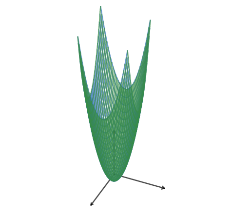
Figure 8: The graph of $f=x^{2}+y^{2}-1$ with 0-level set the unit circle.

For functions mapping from $\mathbb{R}^{n}\rightarrow\mathbb{R}$, $||Df||$ is simply the vector norm of the gradient since the operator norm measures the greatest expansion of any unit vector that occurs under $Df$, which occurs exactly in the direction of the gradient. Thus, $\nabla f=(2x\mathord{}\mathchar 44\relax 2y)\mathord{}\mathchar 44\relax$ and $|\nabla f|=2\sqrt{x^{2}+y^{2}}.$ If we consider $B(0\mathord{}\mathchar 44\relax 1)$ to be closed, then we shall set $B(0\mathord{}\mathchar 44\relax 2R)=B(0\mathord{}\mathchar 44\relax 2).$

$$\lim_{k\rightarrow\infty}\left\{\frac{1}{k}\int_{B(0\mathord{}\mathchar 44\relax 2R)}\left(\frac{||Df||}{|f|}\right)^{\frac{k-1}{k}}d\vec{x}\right\} =2\lim_{k\rightarrow\infty}\left\{\frac{1}{k}\int_{B(0\mathord{}\mathchar 44\relax 2)}\left(\frac{\sqrt{x^{2}+y^{2}}}{x^{2}+y^{2}-1}\right)^{\frac{k-1}{k}}dxdy\right\}$$

$$=2\lim_{k\rightarrow\infty}\left\{\frac{1}{k}\int_{B(0\mathord{}\mathchar 44\relax 1)}\left(\frac{\sqrt{x^{2}+y^{2}}}{1-x^{2}-y^{2}}\right)^{\frac{k-1}{k}}dxdy\right\}$$

$$+2\lim_{k\rightarrow\infty}\left\{\frac{1}{k}\int_{B(0\mathord{}\mathchar 44\relax 2)\setminus B(0\mathord{}\mathchar 44\relax 1)}\left(\frac{\sqrt{x^{2}+y^{2}}}{x^{2}+y^{2}-1}\right)^{\frac{k-1}{k}}dxdy\right\}$$

$$=2\lim_{k\rightarrow\infty}\left\{\frac{1}{k}\int_{0}^{2\pi}\int_{0}^{1}\left(\frac{r}{1-r^{2}}\right)^{\frac{k-1}{k}}rdrd\theta\right\}$$

$$+2\lim_{k\rightarrow\infty}\left\{\frac{1}{k}\int_{0}^{2\pi}\int_{1}^{2}\left(\frac{r}{r^{2}-1}\right)^{\frac{k-1}{k}}rdrd\theta\right\}$$ (13)

Using numerical integration techniques, we find the value of (13) rapidly converging to $4\pi\approx 12.566$ as predicted. For example, with $k=1000$, we have

$$2\lim_{k\rightarrow\infty}\left\{\frac{1}{1000}\int_{0}^{2\pi}\int_{0}^{1}\left(\frac{r}{1-r^{2}}\right)^{\frac{999}{1000}}rdrd\theta\right\}$$

$$+ 2\lim_{k\rightarrow\infty}\left\{\frac{1}{1000}\int_{0}^{2\pi}\int_{1}^{2}\left(\frac{r}{r^{2}-1}\right)^{\frac{999}{1000}}rdrd\theta\right\}$$

$$\approx 12.568.$$

For an analytic solution, Mathematica^® provides the following solution to (13).

$$2\lim_{k\rightarrow\infty}\left\{\frac{1}{k}\int_{0}^{2\pi}\int_{0}^{1}\left(\frac{r}{1-r^{2}}\right)^{\frac{k-1}{k}}rdrd\theta\right\}+2\lim_{k\rightarrow\infty}\left\{\frac{1}{k}\int_{0}^{2\pi}\int_{1}^{2}\left(\frac{r}{r^{2}-1}\right)^{\frac{k-1}{k}}rdrd\theta\right\}$$

$$=2\pi\lim_{k\rightarrow\infty}\left\{\frac{1}{k}\ \frac{2^{\frac{-1}{k}}\Gamma\left(\frac{3}{2}-\frac{1}{2k}\right)\Gamma\left(\frac{1}{k}\right)}{\Gamma\left(\frac{1}{2}\left(3+\frac{1}{k}\right)\right)}\right\}$$

$$+2\pi\lim_{k\rightarrow\infty}\left\{\frac{1}{k}\ \Gamma\left(-\frac{k+1}{2k}\right)\left[\frac{2^{\frac{-1}{k}}\Gamma\left(\frac{1}{k}\right)}{\Gamma\left(\frac{1}{2}\left(\frac{1}{k}-1\right)\right)}-2\,{}_{2}\tilde{F}_{1}\left(\frac{k-1}{k}\mathchar 44\relax\,-\frac{k+1}{2k};\,\frac{k-1}{2k};\,\frac{1}{4}\right)\right]\right\}$$

$$=2\pi\lim_{k\rightarrow\infty}\left\{\frac{1}{k}\ 2^{\frac{-1}{k}}\Gamma\left(\frac{1}{k}\right)\right\}$$

$$+2\pi\lim_{k\rightarrow\infty}\left\{\frac{1}{k}\ \left[2^{\frac{-1}{k}}\Gamma\left(\frac{1}{k}\right)-2\Gamma\left(\frac{-1}{2}\right)\,{}_{2}\tilde{F}_{1}\left(1\mathchar 44\relax\,\frac{-1}{2};\,\frac{1}{2};\,\frac{1}{4}\right)\right]\right\}$$

$$=2\pi\lim_{k\rightarrow\infty}\left\{1+1-\frac{2}{k}\Gamma\left(\frac{-1}{2}\right)\frac{-2+\text{coth}^{-1}(2)}{2\sqrt{\pi}}\right\}$$

$$=2\pi\lim_{k\rightarrow\infty}\left\{1+1-\frac{2}{k}(-2\sqrt{\pi})(.409\dots)\right\}$$

$$=4\pi$$

We note that the regularized hypergeometric function

$${}_{2}\tilde{F}_{1}(b\mathord{}\mathchar 44\relax a;c;z)\equiv\frac{{}_{2}F_{1}(a\mathord{}\mathchar 44\relax b;c;z)}{\sqrt{\pi}}\mathord{}\mathchar 44\relax$$

where ${}_{2}F_{1}(a\mathord{}\mathchar 44\relax b;c;z)$ is the hypergeometric function, which in turn is defined by the power series

$$\sum_{n=0}^{\infty}\frac{(a)_{n}(b)_{n}}{(c)_{n}}\frac{z^{n}}{n!}.$$

Here $|z|<1$ and $(q)_{n}$ is the rising Pochhammer symbol defined by

$$(q)_{n}=\left\{\begin{array}[]{rcl}1&n=0\\ q(q+1)\cdots(q+n-1)&n>0.\end{array}\right.$$

Further, note above that $\lim_{k\rightarrow\infty}\left\{\frac{1}{k}\Gamma\left(\frac{1}{k}\right)\right\}=1.$

6 A $C^{1}$ Boundary Measure for $n=2$

We next present the second main result, that of computing the $\mathcal{H}^{1}$-measure of an embedded $C^{1}$ submanifold in $\mathbb{R}^{2}$ using the singular integral in (5) above.

Theorem 6.1.

Let $f(x)=\inf\{|x-y|\ |\ y\in A\}:\mathbb{R}^{2}\rightarrow\mathbb{R}$ be the distance function to $A\subset\mathbb{R}^{2}$. Further, suppose $A$ is a $C^{1}$ closed embedded 1-dimensional submanifold of $\mathbb{R}^{2}$ such that $A\subset B(0\mathord{}\mathchar 44\relax R)$ (closed) and $\mathcal{H}^{1}(A)<\infty$. Then we have

$$\lim_{k\rightarrow\infty}\left\{\frac{1}{k}\int_{B(0\mathord{}\mathchar 44\relax 2R)}\left(\frac{|Df|}{|f|}\right)^{\frac{k-1}{k}}dy\right\}=2\mathcal{H}^{1}(A).$$ (14)

Proof.

As $A$ is a closed submanifold, i.e. it is compact without boundary, we assume $A\neq\emptyset\mathord{}\mathchar 44\relax$ which implies that $\mathcal{H}^{1}(A)>0.$ We also note that $|Df|\equiv 1\ \mathcal{H}^{2}$-a.e.; $Df$ is undefined on $A$ itself; and that $A$ being $C^{1}$ means that $A$ is locally the graph of a $C^{1}$ function $g:\mathbb{R}\rightarrow\mathbb{R}$.

1. 1. Since $A$ is an embedded submanifold, then globally speaking, no matter how close one portion of $A$ comes to another portion, there is always at least a distance $\eta^{*}>0$ between them. We will chose $\eta$ below in such a way that $\eta\leq\eta^{*}/4$ so that we may cover $A$ with rectangles extending outward $\eta$ on both sides without overlapping (see Figure 9).
      

      Figure 9: Global distance of $A$ to itself.

   2. Since $A$ is a compact submanifold of $\mathbb{R}^{2}$, it is a compact set in $\mathbb{R}^{2}$, hence we can cover $A$ with a finite number of closed disks $B(x_{i}\mathord{}\mathchar 44\relax\delta)$ with $x_{i}\in A$ for $i=1\mathord{}\mathchar 44\relax 2\mathord{}\mathchar 44\relax\dots\mathord{}\mathchar 44\relax M(\delta)\mathord{}\mathchar 44\relax$ where $\delta$ is the fineness of our cover and $M(\delta)$ is the number of disks. Since $A$ is $C^{1}$, for each $x_{i}$, we define $T_{i}\equiv T_{x_{i}}A\cap B(x_{i}\mathord{}\mathchar 44\relax\delta)$, the portion of the linear approximation to $A$ at the point $x_{i}$ contained in each ball $B(x_{i}\mathord{}\mathchar 44\relax\delta)$, which is naturally a diameter of $B(x_{i}\mathord{}\mathchar 44\relax\delta)$ and thus has length $2\delta$ (see Figure 10).

      Figure 10: Covering $A$ with disks $B(x_{i}\mathord{}\mathchar 44\relax\delta)$.

   3. Using the fact that $f$ is continuous on the compact set $B(0\mathord{}\mathchar 44\relax 2R)$ and that $|Df|\equiv 1$ $\mathcal{H}^{2}$-a.e., we see that the integrand in (14) is bounded outside of a neighborhood $E$ of $A$ contained in $B(0\mathord{}\mathchar 44\relax 2R)$ (see Figure 11). Thus we have

      $$\lim_{k\rightarrow\infty}\left\{\frac{1}{k}\int_{B(0\mathord{}\mathchar 44\relax 2R)}\left(\frac{|Df|}{|f|}\right)^{\frac{k-1}{k}}dy\right\}=\lim_{k\rightarrow\infty}\left\{\frac{1}{k}\int_{E}\left(\frac{|Df|}{|f|}\right)^{\frac{k-1}{k}}dy\right\}.$$ (15)

      Figure 11: The $1/k$ sends everything outside $E$ to 0 in the limit.

2. 1. Let $E_{i}^{\eta}$ be a rectangle that is centered on $T_{i}$ with height $2\eta$ and width $2\delta$ for $i=1\mathord{}\mathchar 44\relax 2\mathord{}\mathchar 44\relax\dots\mathord{}\mathchar 44\relax M(\delta)$ and with $\eta$ chosen as above. We will integrate in (14) over each $E_{i}^{\eta}$ and sum the results so that we can use the normals $\vec{N}$ to each $T_{i}$ to approximate the normals $\vec{n}$ to $A\cap E_{i}^{\eta}$. However, we need to bound how much “overlap” there is between the $E_{i}^{\eta}$’s so that the integral over the collection $\{E_{i}^{\eta}\}_{i=1}^{M(\delta)}$ converges to the integral over $\cup_{i=1}^{M(\delta)}E_{i}^{\eta}$ as $\delta\rightarrow 0.$ We do this in the following way, noting that since $A\subset\cup_{i=1}^{M(\delta)}E_{i}^{\eta}\subset B(0\mathord{}\mathchar 44\relax 2R)$, we can apply (15) above (see Figure 12).

      Figure 12: Covering $A$ with rectangles $E^{\eta}_{i}$.

   2. Let $w\mathord{}\mathchar 44\relax z\in A$ and $\alpha>0$. By the uniform continuity of $Dg$, (locally) we can choose $\delta$ small enough so that

      $$|w-z|<\delta\Rightarrow|D_{w}g-D_{z}g|<\alpha.$$

      But this implies that

      $$|g(w)-g(z)|<\alpha\delta\equiv\epsilon.$$

      We pick $\delta$ small enough so that letting $\eta\equiv\sqrt{\alpha}\delta\mathord{}\mathchar 44\relax$ we still have $\eta\leq\eta^{*}/4$ from above. Then

      $$\frac{\eta}{\epsilon}=\frac{\sqrt{\alpha}\delta}{\alpha\delta}=\frac{1}{\sqrt{\alpha}}\rightarrow\infty$$

      as $\alpha\mathord{}\mathchar 44\relax\delta\rightarrow 0$.

      Similarly,

      $$\frac{\delta}{\eta}=\frac{\delta}{\sqrt{\alpha}\delta}=\frac{1}{\sqrt{\alpha}}\rightarrow\infty$$ (16)

      as $\alpha\mathord{}\mathchar 44\relax\delta\rightarrow 0$.

      Lastly, we have

      $$\frac{\delta}{\epsilon}=\frac{\delta}{\alpha\delta}=\frac{1}{\alpha}\rightarrow\infty$$ (17)

      as $\alpha\mathord{}\mathchar 44\relax\delta\rightarrow 0$.

      By the geometric definition of the derivative [8], we observe that $A\cap E_{i}^{\eta}$ is contained in a cone $K_{i}^{\epsilon}$ centered on $x_{i}$ and $T_{i}$ of max height 2$\epsilon$ (at a distance $\delta$ from $x_{i}$ along $T_{i}$) and angular width $2\theta$ (see Figure 13).

   Figure 13: For each $x_{i}\mathchar 44\relax A\cap E^{\eta}_{i}$ is contained the cone $K^{\epsilon}_{i}$. Note that the image is not drawn to scale since $\delta\gg\eta\gg\epsilon.$

3. 1. We now specify the manner in which we cover $A$ with disks, and thus with $E_{i}^{\eta}$’s. We wish for the “overlaps” of the $E_{i}^{\eta}$’s to contain at least an $\eta/2$-neighborhood of $A$, and we want

      $$\mathcal{H}^{2}(E_{i}^{\eta}\cap E_{j}^{\eta})\leq(2\eta)^{2}=4\eta^{2}\mathchar 44\relax\ \ i\neq j.$$

      By choosing $\delta$ small enough, we can arrange each $E_{i}^{\eta}$ so that it intersects with its neighbors only in the $2\eta$-squares on each end of each rectangle $E_{i}^{\eta}$ (see Figure 14).

      More precisely,

      $$\mathcal{H}^{2}(E_{i}^{\eta})=2\delta 2\eta\gg 4\eta^{2}\geq\mathcal{H}^{2}(E_{i}^{\eta}\cap E_{j}^{\eta})\mathchar 44\relax\ \ i\neq j\mathchar 44\relax$$

      since (16) above implies

      $$\delta\gg\eta.$$

      Thus sending $\delta$ to 0 will send the total area of the pairwise “overlap” of the $E_{i}^{\eta}$’s to 0 faster than the area of the collection $\{E_{i}^{\eta}\}_{i=1}^{M(\delta)}$ goes to 0.

      Figure 14: Overlaying $A$ with $E^{\eta}_{i}$’s

   2. We set

      $$I=\frac{1}{k}\int_{\Omega}\left(\frac{|Df|}{|f|}\right)^{\frac{k-1}{k}}dz\mathord{}\mathchar 44\relax$$

      where $\Omega\equiv\{E_{i}^{\eta}\cap E_{j}^{\eta}\}_{i\neq j}\mathord{}\mathchar 44\relax$ the collection of “overlap” of all the $E_{i}^{\eta}$’s taken pairwise. Now we can write

      $$\lim_{k\rightarrow\infty}\left\{\frac{1}{k}\int_{\cup_{i=1}^{M(\delta)}E_{i}^{\eta}}\left(\frac{|Df|}{|f|}\right)^{\frac{k-1}{k}}dz\right\}$$

      $$=\lim_{k\rightarrow\infty}\left\{\frac{1}{k}\int_{\{E_{i}^{\eta}\}_{i=1}^{M(\delta)}}\left(\frac{|Df|}{|f|}\right)^{\frac{k-1}{k}}dz-I\right\}$$

      $$=\lim_{k\rightarrow\infty}\left\{\frac{1-\lambda}{k}\int_{\{E_{i}^{\eta}\}_{i=1}^{M(\delta)}}\left(\frac{|Df|}{|f|}\right)^{\frac{k-1}{k}}dz\right\}$$

      since $I$ is some fraction $0\leq\lambda\equiv\lambda(\delta)<1$ of the same integral taken over the whole (finite) collection $\{E^{\eta}_{i}\}_{i=1}^{M(\delta)}$. Based on the argument just given, $\lambda\rightarrow 0$ as $\delta\rightarrow 0$.

4. 1. We now wish to find bounds on $f$ by showing that the normals to $A\cap E_{i}^{\eta}$ converge to the normals to $T_{i}$ as $\delta\rightarrow 0$. The key lemma here is as follows:

      Lemma 6.1.

      Let $\epsilon>\epsilon^{*}>0$ and let $K^{\epsilon}_{i}$ be the cone of angular width $2\theta$ centered on $x\in T_{i}$ containing $A\cap E_{i}^{\eta}$. There exists a cone $C^{\epsilon^{*}}_{i}$ such that we may translate it (without tipping) along $A\cap E_{i}^{\eta}$ so that $A$ is contained inside $C^{\epsilon^{*}}_{i}$ for all points of $A$ within $\delta^{*}<\delta$ of its center point (see Figure 15).

      Proof.

      Let $\delta>0$ be as above and $w\mathord{}\mathchar 44\relax z\in A\cap E^{\epsilon}_{i}$. Then from the uniform continuity of $Dg$, we find that $|w-z|<\delta$ implies $\angle(D_{w}g\mathord{}\mathchar 44\relax D_{z}g)\leq 2\theta$, that is the angle between $D_{w}g$ and $D_{z}g$ is bounded by $2\theta$, which defines the angular width of $K^{\epsilon}_{i}$. Thus the normals $\vec{n}$ to $A\cap E^{\epsilon}_{i}$ can only deviate from the normals $\vec{N}$ to $T_{i}$ by at most $\theta=\tan^{-1}(\frac{\epsilon}{\delta})$.

      Now, let $a\in A\cap E^{\epsilon}_{i}$ and let $\vec{N}(x)$ be the normal to $T_{i}$ containing $a$. Pick a point $z=(x\mathord{}\mathchar 44\relax t)\in\vec{N}(x)$, where $t\leq\epsilon$ and draw the line segments through $z$ on each side of $\vec{N}(x)$ forming an angle $\theta$ with $\vec{N}(x)$. Without loss of generality, pick one of these segments and label its intersection with $A$ as $\hat{a}\in A\cap E^{\epsilon}_{i}$. We find, from the above argument, that $\vec{n}(\hat{a})$, the normal to $\hat{a}$, cannot deviate from its corresponding $\vec{N}(\hat{x})$ by more than $\theta$, and thus $\angle(D_{a}g\mathord{}\mathchar 44\relax D_{\hat{a}}g)\leq 2\theta$. But this implies that $\hat{a}$ must be inside the cone $C^{\epsilon^{*}}_{i}$ centered on $a$ whose center line $l$ is parallel to $T_{i}$.

      Letting $z=(x\mathord{}\mathchar 44\relax t)$ be any point along $\vec{N}(x)$ with $t\leq\epsilon$, we find that the corresponding $\hat{a}\in C^{\epsilon^{*}}_{i}$, which proves the assertion. We observe that from (17), as $\delta\rightarrow 0\mathchar 44\relax\theta$ also goes to 0.

      ∎

   2. As shown in Figure 15, using our lemma we wish to bound $f(z)$ for $z=(x\mathord{}\mathchar 44\relax t)\in E_{i}^{\eta}$ such that $x\in T_{i}$ and $t\in[-\eta\mathord{}\mathchar 44\relax\eta]$ is the distance to $x$ in the direction of the normal $\vec{N}(x)$ to $T_{i}$. But if we translate $C^{\epsilon^{*}}_{i}$ to each $z\in A\cap E_{i}^{\eta}$ (keeping its center line $l$ parallel to $T_{i}$), we find (with $0\leq\theta<\pi/2$)

      $$\cos(\theta)|t^{*}|\leq|f(z^{*})|\leq|t^{*}|\mathchar 44\relax$$

      which implies

      $$\frac{1}{|t^{*}|}\leq\frac{1}{|f(z^{*})|}\leq\frac{1}{\cos(\theta)|t^{*}|}.$$ (18)

      Here, $z^{*}=(x\mathord{}\mathchar 44\relax t^{*})$, where $t^{*}$ represents the distance from $z=(x\mathord{}\mathchar 44\relax t)$ to $a\in A$ along the normal $\vec{N}(x)$ instead of the distance to $x\in T_{i}$. The actual distance $t$ to $T_{i}$ is either $t^{*}+\beta$ or $t^{*}-\beta$, where $0\leq\beta\leq\epsilon$, depending on what side of $T_{i}$ $a$ is and since $A$ is contained in $K^{\epsilon}_{i}$.

      Figure 15: Translating $C^{\epsilon^{*}}_{i}$ along $A$ so that line $l$ is always parallel to $T_{i}$ and $t^{*}$ is the distance from $z$ to $a$.

      Now, we wish to integrate $1/|f(z)|$ over $[-\eta\mathord{}\mathchar 44\relax\eta]$, with $\eta$ being measured from $T_{i}$, but to use our bound in (18), we make the substitution $z^{*}=(x\mathord{}\mathchar 44\relax t)\pm(0\mathord{}\mathchar 44\relax\beta_{x})$, with $t^{*}=t\pm\beta_{x}$, so that $dz^{*}=dz$ and $dt^{*}=dt$. Note that the points $(x\mathord{}\mathchar 44\relax t)$ and $(x\mathord{}\mathchar 44\relax t^{*})$ represent the same point in $\mathbb{R}^{2}$, but when integrating, we will have different bounds in the integral since our datum is different if our point $a\in A$ is not also in $T_{i}$, that is if $a\neq x$. Therefore, in the case when $a$ is above $T_{i}$, we let our bounds be $\hat{\mathbf{\eta}}^{+}_{x}=\eta-\beta_{x}$ and $\hat{\mathbf{\eta}}^{-}_{x}=-(\eta+\beta_{x})\mathord{}\mathchar 44\relax$ where $\beta_{x}$ depends on $x\in T_{i}$. In the case when $a$ is below $T_{i}$, we have $\hat{\mathbf{\eta}}^{+}_{x}=\eta+\beta_{x}$ and $\hat{\mathbf{\eta}}^{-}_{x}=-(\eta-\beta_{x})$ (see Figure 16).

      Figure 16: On the left, we integrate $1/|f(z)|=1/|f(x\mathord{}\mathchar 44\relax t)|$ over $[-\eta\mathord{}\mathchar 44\relax\eta]$ with $t$ measured as the distance from $x\in T_{i}$. On the right, we integrate $1/|f(z^{*})|=1/|f(x\mathord{}\mathchar 44\relax t^{*})|$ over $[\hat{\mathbf{\eta}}^{-}_{x}\mathord{}\mathchar 44\relax\hat{\mathbf{\eta}}^{+}_{x}]$ with $t^{*}$ measured as the distance from $a\in l$. Both are for the case where $a$ is above $T_{i}$.

      In either case, we are integrating over the same interval. Since all terms in (18) are positive, this will be greater than integrating over $t\in[-(\eta-\epsilon)\mathord{}\mathchar 44\relax\eta-\epsilon]$ and less than integrating over $t\in[-(\eta+\epsilon)\mathord{}\mathchar 44\relax\eta+\epsilon]$, and we have

      $$\int_{-\eta}^{\eta}\left(\frac{1}{|f(z)|}\right)^{\frac{k-1}{k}}dz =\int_{\hat{\mathbf{\eta}}^{-}_{x}}^{\hat{\mathbf{\eta}}^{+}_{x}}\left(\frac{1}{|f(z^{*})|}\right)^{\frac{k-1}{k}}dz^{*}$$

      $$\leq\int_{\hat{\mathbf{\eta}}^{-}_{x}}^{\hat{\mathbf{\eta}}^{+}_{x}}\left(\frac{1}{\cos(\theta)|t^{*}|}\right)^{\frac{k-1}{k}}dt^{*}$$

      $$\leq\int_{-(\eta+\epsilon)}^{\eta+\epsilon}\left(\frac{1}{\cos(\theta)|t|}\right)^{\frac{k-1}{k}}dt\mathchar 44\relax$$

      where $k=1\mathord{}\mathchar 44\relax 2\mathord{}\mathchar 44\relax 3\mathord{}\mathchar 44\relax\dots$. Similarly,

      $$\int_{-\eta}^{\eta}\left(\frac{1}{|f(z)|}\right)^{\frac{k-1}{k}}dz =\int_{\hat{\mathbf{\eta}}^{-}_{x}}^{\hat{\mathbf{\eta}}^{+}_{x}}\left(\frac{1}{|f(z^{*})|}\right)^{\frac{k-1}{k}}dz^{*}$$

      $$\geq\int_{\hat{\mathbf{\eta}}^{-}_{x}}^{\hat{\mathbf{\eta}}^{+}_{x}}\left(\frac{1}{|t^{*}|}\right)^{\frac{k-1}{k}}dt^{*}$$

      $$\geq\int_{-(\eta-\epsilon)}^{\eta-\epsilon}\left(\frac{1}{|t|}\right)^{\frac{k-1}{k}}dt.$$ (19)

5. Putting this all together, we now have that

   $$\lim_{k\rightarrow\infty}\left\{\frac{1}{k}\int_{B(0\mathord{}\mathchar 44\relax 2R)}\left(\frac{|Df|}{|f|}\right)^{\frac{k-1}{k}}dz\right\}$$

   $$=\lim_{k\rightarrow\infty}\left\{\frac{1}{k}\int_{\cup_{i=1}^{M(\delta)}E_{i}^{\eta}}\left(\frac{|Df|}{|f|}\right)^{\frac{k-1}{k}}dz\right\}$$

   $$=\lim_{k\rightarrow\infty}\left\{\frac{1}{k}\int_{\{E_{i}^{\eta}\}_{i=1}^{M(\delta)}}\left(\frac{|Df|}{|f|}\right)^{\frac{k-1}{k}}dz-I\right\}$$

   $$=\lim_{k\rightarrow\infty}\left\{\frac{1-\lambda}{k}\sum_{i=1}^{M(\delta)}\int_{E_{i}^{\eta}}\left(\frac{1}{|f|}\right)^{\frac{k-1}{k}}dz\right\}$$

   $$=\lim_{k\rightarrow\infty}\left\{\frac{1-\lambda}{k}\sum_{i=1}^{M(\delta)}\int_{T_{i}}\int_{-\eta}^{\eta}\left(\frac{1}{|f|}\right)^{\frac{k-1}{k}}dt\,d\mathcal{H}^{1}(x)\right\}$$

   $$\leq\lim_{k\rightarrow\infty}\left\{\frac{1-\lambda}{k}\sum_{i=1}^{M(\delta)}\int_{T_{i}}\int_{-(\eta+\epsilon)}^{\eta+\epsilon}\left(\frac{1}{\cos(\theta)|t|}\right)^{\frac{k-1}{k}}dt\,d\mathcal{H}^{1}(x)\right\}$$

   $$=\lim_{k\rightarrow\infty}\left\{\frac{1-\lambda}{k}\int_{-(\eta+\epsilon)}^{\eta+\epsilon}\left(\frac{1}{|t|}\right)^{\frac{k-1}{k}}dt\left(\frac{1}{\cos(\theta)}\right)^{\frac{k-1}{k}}\sum_{i=1}^{M(\delta)}\int_{T_{i}}d\mathcal{H}^{1}(x)\right\}$$

   $$=\lim_{k\rightarrow\infty}\left\{\frac{1-\lambda}{k}\int_{-(\eta+\epsilon)}^{\eta+\epsilon}\left(\frac{1}{|t|}\right)^{\frac{k-1}{k}}dt\right\}\lim_{k\rightarrow\infty}\left\{\left(\frac{1}{\cos(\theta)}\right)^{\frac{k-1}{k}}\sum_{i=1}^{M(\delta)}\mathcal{H}^{1}(T_{i})\right\}$$

   $$=2(1-\lambda)\lim_{k\rightarrow\infty}\left\{(\eta+\epsilon)^{\frac{1}{k}}\right\}\frac{1}{\cos(\theta)}\sum_{i=1}^{M(\delta)}\mathcal{H}^{1}(T_{i})$$

   $$=\frac{2(1-\lambda)}{\cos(\theta)}\sum_{i=1}^{M(\delta)}\mathcal{H}^{1}(T_{i}).$$ (20)

6. We now let $\delta\rightarrow 0$ in (20), since the above process holds for each cover of $A$ we choose according to our procedure. Let $\delta=1/n$ and define the partial sum of the series in (20) above as

   $$S_{n}\equiv\sum_{i=1}^{M(1/n)}\mathcal{H}^{1}(T_{i}).$$

   We see that $\{S_{n}\}$ is monotonically increasing and bounded by $\mathcal{H}^{1}(A)<\infty$ except for an error term. This is due to the fact that in the “overlap” of the $E_{i}^{\eta}$’s, there may be normals to $A$ that intersect more than one $T_{i}$ with the result that a “double-counted” length of at most $2\eta$ will be included in the sum above for each $T_{i}$. For a given $\delta$, this error term is bounded by $2M(\delta)\eta$. Yet we know that $\eta$ goes to 0 faster than $\delta$ goes to 0 (thus while $M(\delta)<\infty$). Therefore, this error term vanishes as $\delta$ gets small enough, and we have that $\{S_{n}\}\rightarrow\mathcal{H}^{1}(A)$.

   Letting $n\rightarrow\infty$ above amounts to letting $\delta\rightarrow 0$, which forces $\theta\mathchar 44\relax\lambda\rightarrow 0$ by our construction above. This gives

   $$\lim_{\delta\rightarrow 0}\left\{\frac{2(1-\lambda)}{\cos(\theta)}\sum_{i=1}^{M(\delta)}\mathcal{H}^{1}(T_{i})\right\}=2\mathcal{H}^{1}(A).$$

   Thus we have shown that

   $$\lim_{k\rightarrow\infty}\left\{\frac{1}{k}\int_{B(0\mathord{}\mathchar 44\relax 2R)}\left(\frac{|Df|}{|f|}\right)^{\frac{k-1}{k}}dx\right\}\leq 2\mathcal{H}^{1}(A).$$

7. Using an analogous reasoning with the bound in (19), we obtain the desired result.

∎

Remark 6.1.

The next reasonable step is to consider whether Theorem 6.1 holds for rectifiable boundaries. While it holds for polygonal boundaries, a relatively simple example shows that simply being rectifiable is not enough (see the Appendix). What about for the boundaries of closed sets of finite perimeter? This question is more delicate and seems best to start with closed connected sets of finite perimeter, whose boundaries are also connected, such that the topological boundary equals the measure theoretic boundary. Let $E$ be such a set. By Theorem 2.7 in [1], we see that if $B(x\mathord{}\mathchar 44\relax r)$, $r>0$, is a ball centered on $x\in\partial E$, then $\partial E\cap B(x\mathord{}\mathchar 44\relax r)$ must be quasi-graph like. That is, $\partial E$ comes into the ball once, passes through $x$, and leaves the ball once. A sensible next step is to prove Theorem 6.1 holds for such a set $E$ whose boundary is locally Lipschitz, i.e. locally $\partial E$ is the graph of a Lipschitz function. We leave this for future work.

7 Appendix

Example 7.1.

Here we construct an example that shows that Theorem 6.1 does not hold in general for sets with rectifiable boundaries. Let $S$ be the open unit square in $\mathbb{R}^{2}$ and let $B(r)$ be the disc of radius $r>0$. First, we construct a sequence $\{r_{m}\}$ with the property such that

$$\frac{|B(r_{m+1})|+|B(r_{m+2})|+|B(r_{m+3})|+\dots}{|B(r_{m})|}\rightarrow 0\,\,\,\text{as }m\rightarrow\infty.$$

Start with $\{s_{k}\}=\frac{1}{2}\mathord{}\mathchar 44\relax\frac{1}{4}\mathord{}\mathchar 44\relax\frac{1}{8}\mathord{}\mathchar 44\relax\dots$ and let $\{\epsilon_{m}\}=\frac{1}{2}\mathord{}\mathchar 44\relax\frac{1}{4}\mathord{}\mathchar 44\relax\frac{1}{8}\mathord{}\mathchar 44\relax\dots$. From $\{s_{k}\}$, we want to construct a sequence $\{s_{k(m)}\}\equiv\{r_{m}\}$ such that for each $m$

$$\frac{|B(r_{m+1})|+|B(r_{m+2})|+|B(r_{m+3})|+\dots}{|B(r_{m})|}<\epsilon_{m}\mathord{}\mathchar 44\relax$$

and then let $\{\epsilon_{m}\}\rightarrow 0.$ Let $\{r_{1}\}=\{s_{1}\}=\frac{1}{2}$ be the first point in $\{r_{m}\}$, but let $\{r_{2}\}=\{s_{3}\}=\frac{1}{8}$ be the second point. This gives

$$\frac{\frac{1}{8^{2}}+\frac{1}{16^{2}}+\frac{1}{32^{2}}+\dots}{\frac{1}{2^{2}}}<\frac{1}{2}\mathord{}\mathchar 44\relax$$

which follows from the fact that without squaring, we have equality, and squaring only reduces the LHS.

Now let $\{r_{3}\}=\{s_{6}\}=\frac{1}{64}$ be the third point. Note that the previous inequality is improved by removing $\frac{1}{16}$ and $\frac{1}{32}$. This time, for $m=2$, we have

$$\frac{\frac{1}{64^{2}}+\frac{1}{128^{2}}+\frac{1}{256^{2}}+\dots}{\frac{1}{8^{2}}}<\frac{1}{4}.$$

We continue in this way, skipping first one point of $\{s_{k}\}$, then two, then three, and so on, so that $\{r_{m}\}=\frac{1}{2}+\frac{1}{8}+\frac{1}{64}+\frac{1}{1024}+\dots.$ In general, for the $m$th point, we choose $r_{m}=s_{(\frac{m^{2}+m}{2})}$. Observe that picking any subsequence $\{r_{m_{j}}\}\subset\{r_{m}\}$ also has the above property.

Now, we enumerate the rational points in $S$ as $\{q_{j}\}_{j=1}^{\infty}$, pick the first rational point $q_{1}$, and draw the closed disc $B(q_{1}\mathord{}\mathchar 44\relax r_{m_{1}})$ with $r_{m_{1}}$ chosen from $\{r_{m}\}$ such that $B(q_{1}\mathord{}\mathchar 44\relax r_{m_{1}})\cap\partial S=\emptyset$ . Let $C_{1}\equiv\partial B(q_{1}\mathord{}\mathchar 44\relax r_{m_{1}})$. Pick the next rational $q_{2}$. If $q_{2}\notin C_{1}$, we pick a smaller radius $r_{m_{2}}<r_{m_{1}}$ from our sequence $\{r_{m}\}$ so that

$$B(q_{2}\mathord{}\mathchar 44\relax r_{m_{2}})\cap\{C_{1}\cup\partial S\}=\emptyset\mathord{}\mathchar 44\relax$$

and

$$3r_{m_{2}}<d(q_{2}\mathchar 44\relax C_{1}\cup\partial S)\mathord{}\mathchar 44\relax$$

where $d(q_{2}\mathchar 44\relax C_{1}\cup\partial S)$ is the distance function from the point $q_{2}$ to the set $C_{1}\cup\partial S$. If $q_{2}\in C_{1}$, then we perturb $q_{2}$ slightly off of $C_{1}$ so that our new point $\hat{q}_{2}\notin C_{1}\cup\partial S.$ We pick $r_{m_{2}}<r_{m_{1}}$ so that

$$B(\hat{q}_{2}\mathord{}\mathchar 44\relax r_{m_{2}})\cap\{C_{1}\cup\partial S\}=\emptyset\mathord{}\mathchar 44\relax$$

and

$$3r_{m_{2}}<d(\hat{q}_{2}\mathchar 44\relax C_{1}\cup\partial S).$$

Define $\mathcal{B}_{1}\equiv B(q_{1}\mathord{}\mathchar 44\relax r_{m_{1}})$ and let the following also hold with $\hat{q}_{2}$ in place of $q_{2}$. If the disc $B(q_{2}\mathord{}\mathchar 44\relax r_{m_{2}})\subset\mathcal{B}_{1}$, then we let $B^{o}(q_{2}\mathord{}\mathchar 44\relax r_{m_{2}})$ be the open disc, and we replace $\mathcal{B}_{1}$ with

$$\mathcal{B}_{2}\equiv\mathcal{B}_{1}\setminus B^{o}(q_{2}\mathord{}\mathchar 44\relax r_{m_{2}}).$$

Otherwise,

$$\mathcal{B}_{2}\equiv\mathcal{B}_{1}\cup B(q_{2}\mathord{}\mathchar 44\relax r_{m_{2}}).$$

Letting $C_{j}\equiv\partial B(q_{j}\mathord{}\mathchar 44\relax r_{m_{j}})$, we can repeat this process for any rational point in our list so that if $q_{j}\notin\cup_{i=1}^{j-1}C_{i}$, we pick $r_{m_{j}}<r_{m_{j-1}}$ from $\{r_{m}\}$ so that

$$B(q_{j}\mathord{}\mathchar 44\relax r_{m_{j}})\cap\{\cup_{i=1}^{j-1}C_{i}\cup\partial S\}=\emptyset\mathord{}\mathchar 44\relax$$

and

$$3r_{m_{j}}<d(q_{j}\mathchar 44\relax\cup_{i=1}^{j-1}C_{i}\cup\partial S).$$

If $q_{j}\in\cup_{i=1}^{j-1}C_{i}$, then we perturb $q_{j}$ in the following way. Draw the ball $B(q_{j}\mathord{}\mathchar 44\relax r_{m_{j-1}})$, which by construction will only intersect the circle containing $q_{j}$. Since we have a finite number of circles in $\mathcal{B}_{j-1}$ for all $j$, we know that $\cup_{i=1}^{j-1}C_{i}\cup\partial S$ is a closed set and thus its complement is open. Then we can pick a point $\hat{q}_{j}\in B(q_{j}\mathord{}\mathchar 44\relax r_{m_{j-1}})$ in the complement and a radius $r_{m_{j}}$ from our sequence such that $r_{m_{j}}<{r_{m_{j-1}}}$ and

$$3r_{m_{j}}<d(\hat{q}_{j}\mathord{}\mathchar 44\relax\cup_{i=1}^{j-1}C_{i}\cup\partial S).$$

Again, letting the following also hold with $\hat{q}_{j}$ in place of $q_{j}$, if

$$B(q_{j}\mathord{}\mathchar 44\relax r_{m_{j}})\subset\mathcal{B}_{j-1}\mathord{}\mathchar 44\relax$$

then we replace $\mathcal{B}_{j-1}$ with

$$\mathcal{B}_{j}\equiv\mathcal{B}_{j-1}\setminus B^{o}(q_{j}\mathord{}\mathchar 44\relax r_{m_{j}}).$$

Otherwise,

$$\mathcal{B}_{j}\equiv\mathcal{B}_{{j-1}}\cup B(q_{j}\mathord{}\mathchar 44\relax r_{m_{j}}).$$

Continuing in this way, we construct a set $\mathcal{B}$ such that $S\subseteq\operatorname{clos}({\mathcal{B}})$ and $\partial^{*}\mathcal{B}\equiv\cup_{i=1}^{\infty}C_{i}$, where $\partial^{*}\mathcal{B}$ is the reduced boundary of $\mathcal{B}$.

Lastly, we pick a point $x$ on any circle $C_{i}$, pick $r_{m_{j}}$ smaller than the radius of $C_{i}$, and draw $B(x\mathord{}\mathchar 44\relax r_{m_{j}})$. We know by construction that $B(x\mathord{}\mathchar 44\relax r_{m_{j}})\cap C_{k}=\emptyset$ as long as $i\geq j$, except when $k=i$. Therefore $\mathcal{B}\cap B(x\mathord{}\mathchar 44\relax r_{m_{j}})\cap B(q_{p}\mathchar 44\relax r_{m_{p}})$ is either $\mathcal{B}\cap B(x\mathord{}\mathchar 44\relax r_{m_{j}})$ or it is the empty set so long as $p\geq j$ and $p\neq i$. We see that the density ratios computed to get the approximate normal are perturbed only by discs of radius $r_{m_{j+n}}$, where $n\geq 1$. Using our subsequence $\{r_{m_{j}}\}$ and the property of our ratio above, we have that

$$\frac{|B(r_{m_{j+1}})|+|B(r_{m_{j+2}})|+|B(r_{m_{j+3}})|+\dots}{|B(x\mathord{}\mathchar 44\relax r_{m_{j}})|}<\epsilon_{m_{j}}.$$

Letting ${m_{j}}\rightarrow\infty$, we see that $x$ is on the reduced boundary of the set of circles $\cup_{i=1}^{\infty}C_{i}$ since there exists an approximate normal there. By construction, $\mathcal{B}$ is a set of finite perimeter and is thus rectifiable by Theorem 5.15 in [1]. Thus every point in $S$ is a limit point of $\cup_{i=1}^{\infty}C_{i}$, which implies the distance function from any point in $S$ to $\cup_{i=1}^{\infty}C_{i}$ is 0 and Theorem 6.1 does not hold.

References

- [1] Lawrence C Evans and Ronald F Gariepy. Measure theory and fine properties of functions, volume 5. CRC press, revised edition, 2015.
- [2] Herbert Federer. Curvature measures. Transactions of the American Mathematical Society, 93(3):418–491, 1959.
- [3] Klaus Jänich. Vector analysis. Springer Science & Business Media, 2013.
- [4] Davide La Torre, Matteo Rocca, et al. A characterization of functions. Real Analysis Exchange, 27(2):515–534, 2001.
- [5] Dinh The Luc. Taylor’s formula for functions. SIAM Journal on Optimization, 5(3):659–669, 1995.
- [6] Frank Morgan. Geometric measure theory: a beginner’s guide. Academic Press, fourth edition, 2008.
- [7] Kevin R. Vixie. Geometry from deriviatives: from edges to tubes. Presented May 17, 2013.
- [8] Kevin R. Vixie. An invitation to geometric measure theory: part 1. https://notesfromkevinrvixie.org/category/mathematics/.