Topological dyonic dilaton black holes in AdS spaces

Abstract

We construct a new class of dyonic dilaton black hole solutions in the background of Anti-de Sitter (AdS) spacetime. In order to find an analytical solution which satisfy all the field equations, we should consider the string case where the dilaton coupling is $\alpha=1$. The asymptotic behaviour of the solution ($r\rightarrow\infty$) is exactly AdS, where the dilaton field becomes zero and the metric function reduces to $f(r)\rightarrow-\Lambda r^{2}/3$. In this spacetime, black hole horizons and cosmological horizons, can be a two-dimensional positive, zero or negative constant curvature surface. We study the physical properties of the solution and show that depending on the metric parameters, these solutions can describe black holes with one or two horizons or a naked singularity. We investigate thermodynamics of the solutions by calculating the charge, mass, temperature, entropy and the electric potential of these solutions and disclose that these conserved and thermodynamic quantities satisfy the first law of black hole thermodynamics. We also analyze thermal stability of the solutions and find the conditions for which we have a stable dyonic dilaton black hole.

I Introduction

The first attempt to consider a minimal coupling between the scalar fields and gravity was done by Fisher, who found a static and spherically symmetric solution of the Einstein-massless scalar field equations fisher . A great varieties of the scalar fields have been examined for the different goals. One of the interesting scalar field in the black hole physics is the dilaton field. This scalar field appears in variety theories such as dimensional reductions, low-energy limit of string theory, various models of supergravity. A dilaton field naturally couples to gauge fields and thus can influence various physical phenomena. For instance, the presence of the dilaton field can change the causal structure and asymptotic behavior of the spacetime as well as the stability and thermodynamical features of the charged black holes. Given the asymptotic behavior of black holes, various theories can be defined for understanding their physics as well as the Universe behavior. For instance, a powerful tool to get insight into the strong coupling dynamics of certain field theories by studying classical gravity is AdS/CFT which is a correspondence between the gravity in an AdS spacetime and conformal field theory (CFT) living on the boundary of the AdS spacetime ads . The asymptotically flat dilaton black hole solutions in which the dilaton field is coupled to the Maxwell field in an exponential way have been explored in string1 . It was shown that a asymptotically nonflat, non (A)dS solutions can be constructed using one or two Liouville-type dilaton potential string2 . In order to obtain an asymptotically (A)dS solution in the presence of dilaton field, the combination of three Liouville type dilaton potentials were required string3 ; string4 . In this case, the potential includes three exponential dilaton field $(\Phi)$ such as gao1 ; gao2

$$V(\Phi)={\frac{2\Lambda}{3\left({\alpha}^{2}+1\right)^{2}}\left[8\,{\alpha}^{2}{{\rm e}^{\Phi\left(\alpha\,-{{1}/{\alpha}}\right)}}+{\alpha}^{2}\left(3\,{\alpha}^{2}-1\right){{\rm e}^{-\,{{2\Phi}/{\alpha}}}}-\left({\alpha}^{2}-3\right){{\rm e}^{2\,\alpha\,\Phi}}\right]},$$ (1)

where $\alpha$ is a constant which determines the strength of the coupling between dilaton field and gauge field. A special case occurs when the coupling constant is $\alpha=1$ that appears in the low energy limit of string action in Einstein’s frame and corresponds to the bosonic sector of the field theory limit of the superstring model ($N=4$ in supergravity) which calls the ”string” conformal gauge string4 . Also the authors of string5 showed that one of the best case in dilaton gravity to obtain the generalized Toda lattices related to Lie algebra is the string case where $\alpha=1$. The properties of electrically charged dilaton black holes in the background of AdS spacetime have been investigated AdSD . If a black hole contains both electric and magnetic charges it is called dyonic black hole. This type of black holes are one of the best objects to study the effect of external magnetic field on superconductors as well as Hall conductance and DC longitudinal conductivity dyonic1 . Also, it has been argued that dyonic black hole in AdS background may be holographic dual of van der Waals fluid with chemical potential dyonic2 and their dual on the conformal boundary of AdS spacetime is the stationary solutions of relativistic magnetohydrodynamics equations dyonic3 .

In the present work, we would like to find asymptotically AdS dyonic black hole solutions in the presence of dilaton field. Many papers are devoted to investigate dilaton dyonic black holes dyonic4 . However, their asymptotic behaviour are neither AdS nor dS. Also, in dyonic5 dyonic black hole in the Kaluza-Klein theory in the presence an additional scalar potential was explored. In the absence of dilaton field, dyonic black holes in the background of AdS spacetime have been investigated in dyonic6 ; drhendi . The solution of massive gravity in the presence of electric and magnetic charges was explored in dyonic7 .

This paper is organized as follows. In section II, we introduce the action and find the basic field equations by varying the action. In section III, we study thermodynamical properties of the solutions. In section IV, thermal stability of the solutions are checked. We finish our paper with closing remarks in section V.

II Action and Lagrangian

The action of Einstein-Maxwell-dilaton gravity in the presence of a dilaton potential is given by

$$S=\frac{1}{16\pi}\int{d^{4}x\sqrt{-g}\Big{(}\mathcal{R}\text{ }-2g^{\mu\nu}\partial_{\mu}\Phi\partial_{\nu}\Phi-V(\Phi)-e^{-2\Phi}F^{2}\Big{)}},$$ (2)

where Ricci scalar curvature is displayed by $\mathcal{R}$ and $F^{2}=F_{\mu\nu}F^{\mu\nu}$ is the usual Maxwell Lagrangian. Also, $V(\Phi)$ is the potential for $\Phi$ which is given by Eq. (1) by considering the string case ($\alpha=1$),

$$V(\Phi)=\frac{\Lambda}{3}\left(4+e^{2\Phi}+e^{-2\Phi}\right)=\frac{2}{3}\Lambda\left(2+\cosh(2\Phi)\right),$$ (3)

where $\Lambda$ is the cosmological constant. The reason for considering the string case ($\alpha=1$) comes from the fact that we could only find an analytical solution in this case and it is impossible to find an analytical solution for an arbitrary $\alpha$ which satisfy all the field equations. One may ignore the dilaton filed, so the potential reduced to $V(\Phi=0)=2\Lambda$ which is the famous term in the action of AdS spaces. Variation of the action (2) respect to the metric, Maxwell and dilaton fields, respectively, eventuate

$${\cal R}_{\mu\nu}=2\partial_{\mu}\Phi\partial_{\nu}\Phi+\frac{1}{2}g_{\mu\nu}V(\Phi)+2e^{-2\Phi}\Big{(}F_{\mu\beta}F_{\nu}^{\beta}-\frac{1}{4}g_{\mu\nu}F^{2}\Big{)},$$ (4)

$$\partial_{\mu}\Big{(}\sqrt{-g}e^{-2\Phi}F^{\mu\nu}\Big{)}=0,$$ (5)

$$\partial_{\mu}\partial^{\mu}\Phi=\frac{1}{4}\frac{\partial V}{\partial\Phi}-\frac{1}{2}e^{-2\Phi}F^{2}.$$ (6)

Since we are going to construct topological static and spherically symmetric black holes in four dimensions, we take the following form for the metric

$$ds^{2}=-f(r)dt^{2}+{dr^{2}\over f(r)}+r^{2}R^{2}(r)d\Omega_{k}^{2},$$ (7)

where $f(r)$ and $R(r)$ are functions of $r$ which should be determined and $d\Omega_{k}^{2}$ is the metric of a $2$-dimensional hypersurface with constant curvature. Hereafter, we take $k=\pm 1,0$, without loss of generality. The explicit form of $d\Omega_{k}^{2}$ is

$$d\Omega_{k}^{2}=\left\{\begin{array}[]{ll}$$d\theta^{2}+\sin^{2}\theta d\phi^{2}$$,\quad\quad\!\!{\rm for}\quad$$k=1$$,&\\ $$d\theta^{2}+\theta^{2}d\phi^{2}$$,\quad\quad\quad{\rm for}\quad$$k=0$$,&\\ $$d\theta^{2}+\sinh^{2}\theta d\phi^{2}$$,\quad{\rm for}\quad$$k=-1$$.&\end{array}\right.$$ (8)

In order to construct dyonic dilaton black hole, we first find the electric and magnetic fields using the Maxwell equation (5). The only nonzero components of the electromagnetic field tensor are

$$F_{tr}=-F_{rt}=\frac{qe^{2\Phi(r)}}{r^{2}R^{2}(r)},$$ (9)

$$F_{\theta\phi}=-F_{\phi\theta}=\left\{\begin{array}[]{ll}$$p\sin\theta$$,\quad\quad\!\!{\rm for}\quad$$k=1$$,&\\ $$p$$,\quad\quad\quad\quad\,{\rm for}\quad$$k=0$$,&\\ $$p\sinh\theta$$,\quad{\rm for}\quad$$k=-1$$.&\end{array}\right.$$ (10)

Here, we denote the electric and magnetic charge by $q$ and $p$, respectively. Using Maxwell electromagnetic tensor, one can find that $F_{tr}$ is the electric field and $F_{\theta\phi}$ is the magnetic field. It is worth noting that the topological structure of the event horizon does not affect the electric field (9), while it affects the functional form of the magnetic field (10). Also, respect to the values of the $r$ the electric field can change, but magnetic field is independent of $r$ in all three topology. In order to find the metric functions, we try to solve two remaining field equations (4) and (6) by considering the metric function (7) and the non-zero components of the electromagnetic tensor (9) and (10). We find the ($tt$) and ($rr$) components of Eq. (4) as follows:

$$Eq_{tt}=\frac{f^{\prime\prime}}{2}+\left(\frac{R^{\prime}}{R}+\frac{1}{r}\right)f^{\prime}-\frac{q^{2}e^{2\Phi}+p^{2}e^{-2\Phi}}{r^{4}R^{4}}+\frac{V(\Phi)}{2}=0,$$ (11)

$$Eq_{rr}=\frac{f^{\prime\prime}}{2}+\left(\frac{R^{\prime}}{R}+\frac{1}{r}\right)f^{\prime}+2\left(\Phi^{\prime}+\frac{r\,R^{\prime\prime}+2R^{\prime}}{r\,R}\right)f-\frac{q^{2}e^{2\Phi}+p^{2}e^{-2\Phi}}{r^{4}R^{4}}+\frac{V(\Phi)}{2}=0,$$ (12)

where the prime denotes derivative with respect to $r$. It is a matter of calculations to show that the subtraction of Eqs. (11) and (12) leads to the following equation,

$$R^{\prime\prime}+\frac{2}{r}R^{\prime}+{\Phi^{\prime}}^{2}~{}R=0.$$ (13)

Now, we make the ansatz

$$R(r)=e^{\Phi(r)}.$$ (14)

Using this ansatz, one can solve Eq. (13), which admits a solution of the form

$$\Phi(r)=\frac{1}{2}\ln\left(1-\frac{b}{r}\right),$$ (15)

where $b$ is the integration constant which is related to the dilaton field so that if we set $b=0$, the dilaton field will be disappeared. In the asymptotic region where $r\rightarrow\infty$, the dilaton field goes to zero. This is an expected result, since our solutions are asymptotically AdS and thus the effects of the dilaton field in the asymptotic region should be removed. Besides, from (15) we see that the solutions only exist for $r>b$. Thus, one may exclude the region $r<0b$ from the spacetime by redefinition of the coordinate $r\rightarrow\rho$ such that $\rho=\sqrt{r^{2}-b^{2}}$. Thus in the new coordinate $\rho=0$ is correspondence to $r=b$, the spacetime is regular for $\rho>0$, and the line elements of the metric may be written as

$$ds^{2}=-f(\rho)dt^{2}+\frac{\rho^{2}\,d\rho^{2}}{(\rho^{2}+b^{2})f(\rho)}+(\rho^{2}+b^{2})R^{2}(\rho)(d\theta^{2}+\sin^{2}\theta\,d\phi^{2}).$$ (16)

In order to find the metric function $f(r)$, we use the ($\phi\phi$) component of Eq. (4) which is written as

$$Eq_{\phi\phi}=\left(\frac{R^{\prime}}{R}+\frac{1}{r}\right)f^{\prime}+\left(\frac{R^{\prime\prime}}{R}+\frac{{R^{\prime}}^{2}}{R^{2}}+\frac{4R^{\prime}}{r\,R}+\frac{1}{r^{2}}\right)f+\frac{q^{2}e^{2\Phi}+p^{2}e^{-2\Phi}}{r^{4}R^{4}}+\frac{V(\Phi)}{2}-\frac{k}{r^{2}\,R^{2}}=0.$$ (17)

Substituting potential (3), the ansatz (14) and the dilaton field (15) in the above equation, one can find

$$f(r)=-\frac{\Lambda r^{2}}{3}\,\left(1-\frac{b}{r}\right)+\,{\frac{{2p}^{2}}{\left(b-2\,r\right)\left(b-r\right)}}-\,{\frac{{2q}^{2}}{\left(b-2\,r\right)r}}+{\frac{2(m-k~{}r)}{b-2\,r}},$$ (18)

where $m$ is the integration constant which is related to the mass of black hole. One can also rewrite the above solution in term of the new coordinate $\rho$ by replacing $r=\sqrt{\rho^{2}+b^{2}}$. In the asymptotic region ($r\rightarrow\infty$), the dominant term in (18) is the cosmological term, $f(r\rightarrow\infty)=-\Lambda r^{2}/3$ which confirms that our solutions are asymptotically AdS. In the absence of the magnetic charge $(p=0)$, our solution reduces to the topological dilaton black hole in AdS spaces for $\alpha=1$ gao1 ; SheAdS2 ; SheAdS3 . Also, in the absence of the dilaton field ($b=0$), the metric (18) reduces to the dyonic black hole in the AdS spacetime Dutta ; drhendi ,

$$f(r)\Big{|}_{b=0}=k-{\frac{m}{r}}-\frac{\Lambda r^{2}}{3}+{\frac{{q}^{2}}{{r}^{2}}}+{\frac{{p}^{2}}{{r}^{2}}}.$$ (19)

The obtained solutions will fully satisfy all components of the field equations provided,

$$m=\frac{b}{2}+\frac{2}{b}\left(q^{2}-p^{2}\right).$$ (20)

This condition indicates that the electric and magnetic charges $(q,p)$ are not independent parameters. Inserting condition (20) in the metric function (18), we find

$$f(r)=k-\frac{\Lambda r^{2}}{3}\,\left(1-\frac{b}{r}\right)-{\frac{2{q}^{2}}{br}}+{\frac{2{p}^{2}}{b\left(r-b\right)}}.$$ (21)

Next we look for the singularity and horizon(s) of the spacetime. The divergency in the Ricci and Kretschmann scalars confirm the existence of the essential singularity. The Ricci scalar is calculated as

$$Ricci=-{\frac{\left({b}^{2}-8br+8{r}^{2}\right)\Lambda}{2\left(b-r\right)r}}-{\frac{b{q}^{2}}{{r}^{3}\left(b-r\right)^{2}}}-{\frac{{p}^{2}b}{{r}^{2}\left(b-r\right)^{3}}}+{\frac{k{b}^{2}}{2{r}^{2}\left(b-r\right)^{2}}}.$$ (22)

As one can see from Eq. (22), the surface $r=b$ $(\rho=0)$ as well as $r=0$ are curvature singularities. Since we have excluded $r<b$ from our spacetime, thus, in our new coordinates, the essential singularity is located at $\rho=0$ ($r=b$). As we already mentioned our solution only exist for $r>b$. The explicit form of the Kretchmann invariant is very complicated and for the economic reasons we do not present it here. It is easy to show that

$$\lim\limits_{\rho\rightarrow 0}R_{\mu\nu\alpha\beta}R^{\mu\nu\alpha\beta}\rightarrow\infty.$$ (23)

From Eqs. (22) and (23), we conclude that there is an essential singularity at $\rho=0$. The behaviour of these scalars in the large $\rho$ limit is interesting, too. At this limit, the dominate term in the Ricci and Kretchmann scalars are given by

$$\lim\limits_{\rho\rightarrow\infty}R_{\mu\nu\alpha\beta}R^{\mu\nu\alpha\beta} \rightarrow \frac{8\Lambda^{2}}{3},$$

$$\lim\limits_{\rho\rightarrow\infty}\rm Ricci \rightarrow 4\Lambda,$$ (24)

which are the characterization of the (A)dS spaces. Now we look for the horizon(s). Black hole horizon(s) is indeed the positive real root of Eq. $f(r)=0$. Unfortunately, it is not easy to find the location of the horizons, analytically. However, we can find the location of horizons by plotting the function $f(r)$ versus $r$. In all figures, we set $\Lambda=-3$. According to Fig. 1 the number of horizons depend on the values of the metric parameters. Our solution may have one or two horizons and in some cases, it may describe a naked singularity depending on the parameters. In summary, our solutions can describe black holes in the case $b<r_{+}$, where $r_{+}$ is the outer horizon of the black string (the largest root of Eq. $f(r)=0$).

In Fig. 1(a) we consider the effect of the horizon topology on the number of horizons. By fixing other metric parameters, the number of horizons decreases by increasing $k$. Figs. 1(b) and 1(c) show that with increasing the value of the magnetic charge, the number of horizons decrease, while by increasing the electric charge the number of horizons can increase, too.

(a) $p=0.5$, $q=0.61$ and $b=0.2$

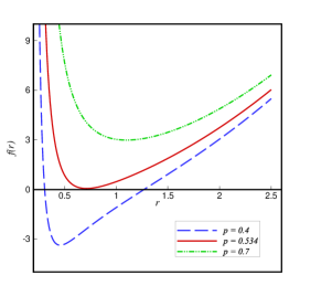
(b) $k=1$, $q=0.7$ and $b=0.2$

(c) $k=1$, $p=0.5$ and $b=0.2$

(d) $k=1$, $p=0.4$ and $q=0.56$

Figure 1: The behavior of the metric function $f(r)$ versus $r$.

III Thermodynamical properties

The Hawking temperature is attributed to the black hole horizon (surface gravity $\kappa$) and is defined as

$$T=\frac{\kappa}{2\pi}=\frac{1}{2\pi}\sqrt{-\frac{1}{2}(\nabla_{\mu}\chi_{\nu})(\nabla^{\mu}\chi^{\nu})},$$ (25)

where $\chi=\partial/\partial t$ is null Killing vector of the horizon. It is a matter of calculation to show

$$T=\frac{f^{\prime}(r)_{|}{{}_{r=r_{+}}}}{4\pi}={\frac{1}{2\pi}\left[{\frac{k}{2r_{{}_{+}}}}-{\frac{{p}^{2}}{r^{3}}\left(1-\frac{b}{r_{{}_{+}}}\right)^{-2}}+\frac{\left(2\,b-3\,r_{{}_{+}}\right)}{6}\Lambda\right]}.$$ (26)

Here

$$r_{+}=\sqrt{\rho_{+}^{2}+b^{2}}$$

shows the outer horizon which is the largest positive real root of $f(r_{+})=0$. It is also interesting to note that in the absence of magnetic charge ($p=0$), it reduces to the temperature of charged AdS dilaton black hole SheAdS3 for $\alpha=1$. The entropy of the dilaton black hole typically obeys the area law of the entropy which is a quarter of the event horizon area Beckenstein . For our solution it is obtained as

$$S=\frac{\Omega_{k}~{}r_{{}_{+}}^{2}}{4}\left(1-\frac{b}{r_{{}_{+}}}\right),$$ (27)

where $\Omega_{k}$ is the volume of the two dimensional hypersurface with constant curvature. The above expression is exactly the entropy of charged AdS dilaton black hole SheAdS3 . Using Brown and York formalism we calculate the mass of the asymptotically AdS dyonic dilaton black hole SheAdS3 . We find

$$M=\frac{\Omega_{k}~{}(q^{2}-p^{2})}{4~{}b\pi}=\frac{\Omega_{k}}{8\pi}\left(m-\frac{b}{2}\right).$$ (28)

In the absence of magnetic charge ($p=0$), it recovers the mass of the AdS dilaton black hole SheAdS3 , while in the absence of dilaton field ($b=0$), it reduces to the mass of topological dyonic AdS black holes. One may use the Gauss’s law to calculate the total electric and magnetic charge of the black hole. According to the Gauss theorem, the electric charge of the black hole is

$$Q=\frac{1}{4\pi}\int_{r\rightarrow\infty}\sqrt{-g}F_{tr}d^{2}x=\frac{q\Omega_{k}}{4\pi}.$$ (29)

Similarly, we can obtain the total magnetic charge of the dyonic black hole as

$$P=\frac{p\Omega_{k}}{4\pi}.$$ (30)

Also, one can obtain $U_{{}_{Q}}$ and $U_{{}_{P}}$ which are, respectively, the electric and magnetic potential by applying their definition using the free energy, which is given as Dutta

$$W=\frac{I_{\rm onshell}}{\beta}$$ (31)

where $I_{\rm onshell}$ is the on shell action and $\beta$ is the inverse of temperature. Multiplying both sides of Eq. (4) by $g^{\mu\nu}$, we arrive at

$$\mathcal{R}=2\partial^{\mu}\phi\partial_{\mu}\phi+2V(\Phi).$$ (32)

Substituting Eq. (32) in Eq. (2), we find

$$I_{\rm onshell}=\frac{1}{16\pi}\int{d^{4}x\sqrt{-g}\Big{(}V(\Phi)-e^{-2\Phi}F^{2}\Big{)}}.$$ (33)

As $r$ goes to infinity, the above integration diverges. In order to remove the divergency, one may add some counterterm to the original action or subtracting the contribution of a background spacetime. Finally, we drive the electric and magnetic potential as

$$U_{{}_{Q}}=-\frac{\partial W}{\partial Q}=\frac{Q}{r},$$ (34)

$$U_{{}_{P}}=\frac{\partial W}{\partial P}=\frac{P}{r-b}.$$ (35)

It is important to note that the dialton field does not affect the electric potential, while it changes the magnetic potential. In the absence of the dilaton field ($b=0$), magnetic potential is the same as that in Dutta ; drhendi . In the thermodynamics consideration, the satisfaction of the first law of thermodynamics implies the correctness of conserved and thermodynamic quantities. In order to check this, we obtain the mass $M$ as a function of extensive quantities $S$, $Q$ and $P$. We find

$$M(S,Q,P)=\frac{4\pi}{b}(Q^{2}-P^{2}).$$ (36)

Considering the fact that all thermodynamic quantities should be defined on the horizon, we write $b=b(Q,r,P)$. Taking into account the fact that the entropy is a function of $S=S(r,b)$ and the mass is a function of extensive parameters $M=M(S,Q,P)$, we define the temperature, electric and magnetic potentials as

$$T=\left(\frac{\partial M}{\partial S}\right)_{Q,P}=\frac{\left(\frac{\partial M}{\partial b}\right)_{Q,P}\times dbr}{\left(\frac{\partial S}{\partial r_{{}_{+}}}\right)_{Q,P}+\left(\frac{\partial S}{\partial b}\right)_{Q,P}\times dbr},$$ (37)

$$U_{{}_{Q}}=\left(\frac{\partial M}{\partial Q}\right)_{S,P}+\left(\frac{\partial M}{\partial b}\right)_{S,P}\left(\frac{\partial b}{\partial Q}\right)_{S,P},$$ (38)

$$U_{{}_{P}}=\left(\frac{\partial M}{\partial P}\right)_{S,Q}+\left(\frac{\partial M}{\partial b}\right)_{S,Q}\left(\frac{\partial b}{\partial P}\right)_{S,Q},$$ (39)

where we can compute $dbr$ as

$$dbr=\left(\frac{db}{dr_{{}_{+}}}\right)_{Q,P}=-\frac{\left(\frac{\partial f}{\partial r}\right)_{Q,P}}{\left(\frac{\partial f}{\partial b}\right)_{Q,P}}=\frac{{{\frac{2{q}^{2}}{b{r}^{2}}}-{\frac{2{P}^{2}}{b\left(-r+b\right)^{2}}}-\frac{\Lambda\left(-2r+b\right)}{3}}}{{\frac{2{q}^{2}}{{b}^{2}r}}+{\frac{2P^{2}(-r+2\,b)}{{b}^{2}\left(-r+b\right)^{2}}}+\frac{\Lambda~{}r}{3}}.$$ (40)

Finally, our calculations show that all intensive quantities given in Eqs. (26), (34) and (35) satisfy the first law of black hole thermodynamics,

$$dM=TdS+U_{{}_{Q}}dQ+U_{{}_{P}}dP.$$ (41)

IV Thermal Stability

This section is devoted to study the stability of the dyonic dilaton black holes. Since we consider three extensive variables $X_{i}$, the best way to check the stable range of our solution is to work in the grand- canonical ensemble and study the Hessian matrix hess which is defined as

$$H^{{}^{M}}_{{}_{X_{i}X_{j}}}=\frac{\partial^{2}M}{\partial X_{i}\partial X_{j}}.$$ (42)

Positivity of determinant of the Hessian matrix is sufficient to ensure thermal stability in the grand-canonical ensemble. As mentioned before we may select $X_{i}=(S,Q,P)$. Since the mass is not an explicit function of $X_{i}$, we use the following definitions to obtain the components of the Hessian matrix,

$$H_{11}=\left(\frac{d^{2}M}{d^{2}S}\right)_{P,Q}=\left(\frac{dT}{dS}\right)_{P,Q}=\frac{\left(\frac{\partial T}{\partial r_{{}_{+}}}\right)_{P,Q}+\left(\frac{\partial T}{\partial b}\right)_{P,Q}\times dbr}{\left(\frac{\partial S}{\partial r_{{}_{+}}}\right)_{P,Q}+\left(\frac{\partial S}{\partial b}\right)_{P,Q}\times dbr},$$

$$H_{22}=\left(\frac{d^{2}M}{d^{2}P}\right)_{S,Q}=\left(\frac{dM_{P}}{dP}\right)_{S,Q}=\left(\frac{\partial M_{P}}{\partial P}\right)_{S,Q}+\left[\left(\frac{\partial M_{P}}{\partial r}\right)_{S,Q}\left(\frac{dr_{{}_{+}}}{db}\right)_{S,Q}+\left(\frac{\partial M_{P}}{\partial b}\right)_{S,Q}\right]\left(\frac{dP}{db}\right)^{-1}_{S,Q},$$

$$H_{33}=\left(\frac{d^{2}M}{d^{2}Q}\right)_{S,P}=\left(\frac{dM_{Q}}{dQ}\right)_{S,P}=\left(\frac{\partial M_{Q}}{\partial Q}\right)_{S,P}+\left[\left(\frac{\partial M_{Q}}{\partial r}\right)_{S,P}\left(\frac{dr_{{}_{+}}}{db}\right)_{S,Q}+\left(\frac{\partial M_{Q}}{\partial b}\right)_{S,P}\right]\left(\frac{dQ}{db}\right)^{-1}_{S,P},$$

$$H_{12}=H_{21}=\left(\frac{d^{2}M}{dSdP}\right)_{Q}=\left(\frac{dT}{dP}\right)_{S,Q}=\left(\frac{\partial T}{\partial P}\right)_{S,Q}+\left[\left(\frac{\partial T}{\partial r_{{}_{+}}}\right)_{S,Q}\left(\frac{dr_{{}_{+}}}{db}\right)_{S,Q}+\left(\frac{\partial T}{\partial b}\right)_{S,Q}\right]\left(\frac{dP}{db}\right)^{-1}_{S,Q},$$

$$H_{13}=H_{31}=\left(\frac{d^{2}M}{dSdQ}\right)_{P}=\left(\frac{dT}{dQ}\right)_{S,P}=\left[\left(\frac{\partial T}{\partial r_{{}_{+}}}\right)_{S,P}\left(\frac{dr_{{}_{+}}}{db}\right)_{S,P}+\left(\frac{\partial T}{\partial b}\right)_{S,P}\right]\left(\frac{dQ}{db}\right)^{-1}_{S,P}$$

$$H_{23}=H_{32}=\left(\frac{d^{2}M}{dQdP}\right)_{S}=\left(\frac{dM_{Q}}{dP}\right)_{S,Q}$$

$$\indent\indent\indent\,\,\,=\left(\frac{\partial M_{Q}}{\partial P}\right)_{S,Q}+\left[\left(\frac{\partial M_{Q}}{\partial r_{{}_{+}}}\right)_{S,Q}\left(\frac{dr_{{}_{+}}}{db}\right)_{S,Q}+\left(\frac{\partial M_{Q}}{\partial b}\right)_{S,Q}\right]\left(\frac{dP}{db}\right)^{-1}_{S,Q},$$

together with the following definitions

$$M_{Q}=\left(\frac{dM}{dQ}\right)_{S,P}=\left(\frac{\partial M}{\partial Q}\right)_{S,P}+\left(\frac{\partial M}{\partial b}\right)_{S,P}\left(\frac{dQ}{db}\right)^{-1}_{S,P},$$

$$M_{P}=\left(\frac{dM}{dP}\right)_{S,Q}=\left(\frac{\partial M}{\partial P}\right)_{S,Q}+\left(\frac{\partial M}{\partial b}\right)_{S,Q}\left(\frac{dP}{db}\right)^{-1}_{S,Q}.$$ (44)

Using the above definitions, we can calculate the determinant of Eq. (42). The final result is very complex, so we use diagrams to analyze the stability. In all figures we set $\Lambda=-3$.

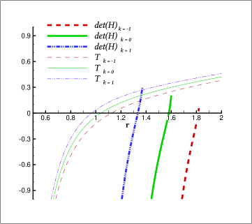
Figure 2: $b=0.2$, $P=1$ and $Q=0.6$.

In Fig. 2, we plot the determinate for all three values of topological constant $k$ respect to $r$. Since a real black hole should have a non-zero value for temperature, so we should have a careful look at the temperature in all considerations. In this figure, the three bold lines refer to the determinate of Hessian matrix which is displayed by det(H) , and the three thin lines relate to the temperature. According to this figure, when we fix the metric parameters, all three temperature functions enjoy a minimum at radius $r_{min_{{}_{T}}}$ for which $r<r_{min_{{}_{T}}}$, this function is negative. Also, one may see a minimum radius for the determinate functions $r_{min_{d}}$ that it is negative in the interval $r<r_{min_{d}}$. When $r_{min_{{}_{T}}}<r<r_{min_{d}}$, the black hole is not thermally stable. This range increases as the values of $k$ decreases. Our calculations show that another special radius exists for the determinate function that we call it ($r_{max_{d}}$) which is the final point in which this function is displayed. We see that when $r>r_{max_{d}}$ the values of determinate functions are imaginary so we can not discuss in this interval using the Hessian matrix. As a result, for a special values of the metric parameters, the black hole experiences a stable state if $r_{min_{d}}<r<r_{max_{d}}$ and this interval changes as metric parameters change, for example by increasing $k$ this stable range increases, too.

(a) $\,r=0.6$

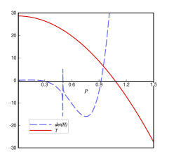
(b) $\,r=1$

Figure 3: $b=0.2$, $k=1$ and $Q=0.5$

In order to better understanding the effects of magnetic charge on the stability, we plot Fig. 3. In this diagram, we fix the radius and allow the magnetic charge $P$ to change. By fixing other metric parameters, one can see that in order to have a real black hole which has positive values of temperature, there exist a maximum for the magnetic charge ($P_{max_{{}_{T}}}$). Also, a divergency in det(H) is observed which corresponds to the equality of charges ($P=Q$). As mentioned before, the positivity of both temperature and Hessian determinate is necessary for stability. Based on the figures, when $P<P_{max_{{}_{T}}}$ the temperature is positive. The curve of det(H) has some special point ($P^{i}_{d}$) in this interval which shows that the curve goes to zero at this point and its sign will change. The numbers of this points increase as we consider the larger radius for black hole. For instance, when $r=0.6$ one special point exist ($P^{1}_{d}$) and the stable interval places at $0<P<P^{1}_{d}$. But for $r=1$, det(H) becomes zero at two points. We call them $P^{1}_{d}$ and $P^{2}_{d}$. Therefore, thermal stability occurs for two smaller intervals ($0<P<P^{1}_{d}$ and $P^{2}_{d}<P<P_{max_{{}_{T}}}$).

In order to determine thermal stability and possible phase transition of the black holes, one may check the heat capacity in fixed values of electric charge. In this case, we work in the canonical ensemble.

$$C_{Q}=T\left(\frac{dS}{dT}\right)_{Q}=\frac{1}{A}\left[3\,\left(-\left(2\,b-3\,r\right)r\left(b-r\right)^{2}\Lambda-3\,\left(b-r\right)^{2}k+6\,{P}^{2}\right){r}^{2}\left(b-r\right)^{2}\left({P}^{2}-{q}^{2}\right)\right],$$ (45)

where one can calculate the denominator as

$$A =\left[-3\,{r}^{2}{b}^{2}\left(b-r\right)^{4}\Lambda-18\,r\left(b-r\right)^{2}\left(2\,b-r\right){P}^{2}-18\,\left(b-r\right)^{4}{q}^{2}\right]k-{r}^{3}\left(b-r\right)^{4}\left(2\,b-r\right){b}^{2}{\Lambda}^{2}$$ (46)

$$+\left[-6\,{r}^{2}\left({b}^{2}+4\,br-3\,{r}^{2}\right)\left(b-r\right)^{2}{P}^{2}-6\,r\left(b-r\right)^{4}\left(2\,b+3\,r\right){q}^{2}\right]\Lambda+36\,r\left(2\,b-3\,r\right){P}^{4}$$

$$-36\,\left(b+3\,r\right)\left(b-r\right){q}^{2}{P}^{2}.$$

As we know, only the positive values of the thermal capacity of a thermodynamic object are acceptable and the negative values show that the object is not real. Also, In black hole physics in the presence of positive temperature, divergency of heat capacity shows that the black hole is not stable and needs a thermodynamical phase transition. We call this transition as type one. Also, zero values of $C_{Q}$ is not acceptable and usually occurs for extremal black holes (which they have zero value for temperature). The black hole may experience another type of phase transition at this point which we call it type two. If the values of heat capacity change to positive ones, it means that the extremal black hole becomes a black hole with two horizons.

Looking at (45), one may find that, regardless of other metric parameters, by choosing equal values for both charges ($Q=P$), this function vanishes. We plot heat capacity and the temperature in Fig.4 to better analyzing. We consider $\Lambda=-3$ in this figure.

(a) $\,Q=0.2$

(b) $\,Q=6$

Figure 4: $b=0.1$, $k=1$ and $P=0.4$

By fixing other metric parameters, Fig.4(a) shows that when the magnetic charge is larger than electric charge ($P>Q$), both types of phase transition occur. The divergency in $C_{Q}$ happens at positive temperature interval. As the values of radius increase, the heat capacity changes from positive to negative values, and thermal phase transition makes the black hole smaller (transition between small and large black hole). That’s because, for large $r$, heat capacity is negative and black hole cannot exist in this range. Choosing smaller values for the magnetic charge ($P<Q$), we only observe the type one of phase transition (see Fig.4(b)). Since the temperature values are also becoming positive, we can deduce that after this point our black hole will have two horizons. Note that for extremal black holes, the temperature is zero. Finally, we conclude that black holes stability are crucially dependent on the metric parameters.

V Closing remarks

In this paper, we have constructed a new class of topological dyonic dilaton black hole solutions in the bachground of AdS spacetime. The only case we could find an analytical solution which fully satisfy all components of the field equations, is the string case where the dilaton coupling constant is taken $\alpha=1$. We have taken the dilaton potential in the form of the combination of three Liouville type introduced in gao1 ; gao2 . By solving the equation of motions, we obtained the solutions which depend on both magnetic and electric charges. We showed that the geometric mass of the black hole and two charges are not independent of each other. Based on the metric parameters, our solutions can be a black hole with two horizons, extremal black hole or a naked singularity. Then, we explored thermodynamics of these topological dilaton black holes and checked the first law of thermodynamics. Finally, we disclosed the effects of metric parameters on the stability of the solutions. There are three extensive parameters (electric charge $Q$, magnetic charge $P$ and entropy $S$) in our theory, it is recommended to use Hessian matrix method to check the stability. The positivity of temperature and the determinate of Hessian matrix simultaneously, ensure that the solution is stable.

We found that the stability of our solutions is closely related to the values of the metric parameters and it is not stable at all interval of $r$. For example, when other metric parameters are fixed, by increasing the value of the topological constant, $k$, the stable interval decreases. Also, for the equal values of electric and magnetic charges, the Hessian method did not work since the determinate diverges.

We also checked the stability in the canonical ensemble, where the electric charge is a fixed parameter. Thus, the positivity of the thermal capacity $C_{Q}$ is sufficient to ensure the local stability. In our theory, we observed that, as other metric parameters are fixed, when $Q<P$, the heat capacity diverges at a special radius and type two of phase transition which coincides with the divergence of $C_{Q}$ (while the temperature is positive) occurs. It is important to note that $C_{Q}$ vanishes by considering equal values for both electric and magnetic charges ($P=Q$) for all radius. Also, we got the type two of phase transition coincides with vanishing of the heat capacity and temperature, and interpreted it as a transition from a non-physical black holes to physical one or a transition from extremal black hole to black hole with two horizons. By choosing $Q>P$ this transition is also observed. As a result, all figures show that, the stability is quite dependent on the metric parameters, and the change of them can alter the black hole stability.