Constrained optimization as ecological dynamics with applications to random quadratic programming in high dimensions

Abstract

Quadratic programming (QP) is a common and important constrained optimization problem. Here, we derive a surprising duality between constrained optimization with inequality constraints – of which QP is a special case – and consumer resource models describing ecological dynamics. Combining this duality with a recent ‘cavity solution’, we analyze high-dimensional, random QP where the optimization function and constraints are drawn randomly. Our theory shows remarkable agreement with numerics and points to a deep connection between optimization, dynamical systems, and ecology.

Optimization is an important problem for numerous disciplines including physics, computer science, information theory, machine learning, and operations research Boyd and Vandenberghe (2004); Bertsekas (1999); Bishop (2006); Mezard and Montanari (2009). Many optimization problems are amenable to analysis using techniques from the statistical physics of disordered systems Zdeborová (2009); Mézard et al. (2002); Moore and Mertens (2011). Over the last few years, similar methods have been used to study community assembly and ecological dynamics suggesting a deep connection between ecological models of community assembly and optimization Fisher and Mehta (2014); Kessler and Shnerb (2015); Dickens et al. (2016); Bunin (2017); Advani et al. (2018); Barbier et al. (2018); Biroli et al. (2018); Tikhonov and Monasson (2017); Marsland III et al. (2018).Yet, the exact relationship between these two fields remains unclear.

Here, we show that constrained optimization problems with inequality constraints are naturally dual to an ecological dynamical system describing a generalized consumer resource model Macarthur and Levins (1967a); MacArthur (1970); Chesson (1990). As an illustration of this duality, we focus on a particular important and commonly encountered constrained optimization problem: Quadratic Programming (QP) Boyd and Vandenberghe (2004). In QP, the goal is to minimize a quadratic objective function subject to inequality constraints. We show that QP is dual to one of the most famous models of ecological dynamics, MacArthur’s Consumer Resource Model (MCRM) – a system of ordinary differential equations describing how species compete for a pool of common resources Macarthur and Levins (1967a); MacArthur (1970); Chesson (1990). We also show that the Lagrangian dual of QP has a natural description in terms of generalized Lotka-Volterra equations that can be derived from the MCRM in the limit of fast resource dynamics.

We then consider random quadratic programming (RQP) problems where the optimization function and inequality constraints are drawn from a random distribution. We exploit a recent ‘cavity solution’ to the MCRM by one of us to construct a mean-field theory for the statistical properties of RQP Advani et al. (2018). Our theory is exact in infinite dimensions and shows remarkable agreement with numerical simulations even for moderately sized finite systems. This duality also allows us to use ideas from ecology to understand the behavior of RQP and interpret community assembly in the MCRM as an optimization problem.

Optimization as ecological dynamics

We begin by deriving the duality between constrained optimization and ecological dynamics. Consider an optimization problem of the form

$$\underset{\mathbf{R}}{\text{minimize}} f({\mathbf{R}})$$ (1)

subject to $$g_{i}({\mathbf{R}})\leq 0,\;i=1,\ldots,S.$$

$$R_{\alpha}\geq 0,\;\alpha=1,\ldots,M.$$

where the variables being optimized ${\mathbf{R}}=(R_{1},R_{2},\ldots,R_{M})$ are constrained to be non-negative. We can introduce a ‘generalized’ Lagrange multiplier $\lambda_{i}$ for each of the $S$ inequality constraints in our optimization problem. In terms of the $\lambda_{i}$, we can write a set of conditions collectively known as the Karush-Kuhn-Tucker (KKT) conditions that must be satisfied at any local optimum ${\mathbf{R}_{min}}$ of our problem Boyd and Vandenberghe (2004); Bertsekas (1999); Bishop (2006). We note that for this reason, in the optimization literature the $\lambda_{i}$ are often called KKT-multipliers rather than Lagrange multipliers. The KKT conditions are:

Stationarity: $\nabla_{\mathbf{R}}f({\mathbf{R}}_{\mathrm{min}})+\sum_{j}\lambda_{j}\nabla_{\mathbf{R}}g_{j}({\mathbf{R}}_{\mathrm{min}})=0$
Primal feasibility: $g_{i}({\mathbf{R}}_{\mathrm{min}})\leq 0$
Dual feasibility: $\lambda_{i}\geq 0$
Complementary slackness: $\lambda_{i}(g_{i}({\mathbf{R}}_{\mathrm{min}})-m_{i})=0$,

where the last three conditions must hold for all $i=1,\ldots,M$. The KKT conditions have a straightforward and intuitive explanation. At the optimum ${\mathbf{R}}_{\mathrm{min}}$, either $g_{i}({\mathbf{R}}_{\mathrm{min}})=0$ and the constraint is active $\lambda_{i}\geq 0$, or $g_{i}({\mathbf{R}}_{\mathrm{min}})\leq 0$ and the constraint is inactive $\lambda_{i}=0$. In our problem, the KKT conditions must be supplemented with the additional requirement of positivity $R_{\alpha}\geq 0$.

One can easily show that the four KKT conditions and positivity are also satisfied by the steady states of the following set of differential equations restricted to the space $\lambda_{i},R_{\alpha}\geq 0$:

$${d\lambda_{i}\over dt} = \lambda_{i}g_{i}({\mathbf{R}})$$

$${dR_{\alpha}\over dt} = [-\partial_{R_{\alpha}}f({\mathbf{R}})-\sum_{j}\lambda_{j}\partial_{R_{\alpha}}g_{j}({\mathbf{R}})]R_{\alpha}$$ (2)

The first of these equations just describes exponential growth of a “species” $i$ with a resource-dependent “growth rate” $g_{i}({\mathbf{R}})$. Species with $g_{i}({\mathbf{R}}_{\mathrm{min}})\leq 0$ correspond to constraints that are inactive and go extinct in the ecosystem (i.e $\lambda_{i\,\mathrm{min}}=0$), whereas species with $g_{i}({\mathbf{R}}_{\mathrm{min}})=0$ survive at steady state and correspond to active constraints with $\lambda_{i\,\mathrm{min}}\neq 0$ (see Figure 1 for a simple two-dimensional example). The second equation in (2) performs a “generalized gradient descent” on the optimization function $f(\mathbf{R})+\sum_{j}\lambda_{j}g_{j}(\mathbf{R})$ (note the extra factor of $R_{\alpha}$ in our dynamics compared to the usual gradient descent equations). In the context of ecology, these equations describe the dynamics of a set of resources $\{R_{\alpha}\}$ produced at a rate $-\partial_{R_{\alpha}}f({\mathbf{R}})R_{\alpha}$ and consumed by individuals of species $j$ at a rate $\lambda_{j}\partial_{\alpha}g_{j}({\mathbf{R}})R_{\alpha}$.

This suggests a simple dictionary for constructing systems dual to optimization problems with inequality constraints (see Figure 1) . The variables are resources whose dynamics are governed by the gradient of the function being optimized. Each inequality is associated with a species through its corresponding Lagrange (KKT) multiplier. Species that survive in the ecosystem correspond to active constraints whereas species that go extinct correspond to inactive constraints. The steady-state values of the resource and species abundances correspond to the local optimum $\mathbf{R}_{\mathrm{min}}$ and Lagrange multipliers at the optimum $\{\lambda_{j\mathrm{\,min}}\}$, respectively. Finally, the $f({\mathbf{R}}_{\mathrm{min}})$ are closely related to Lyapunov functions known to exist in the literature for specific choices of resource dynamics MacArthur (1970); Chesson (1990); Tikhonov and Monasson (2017).

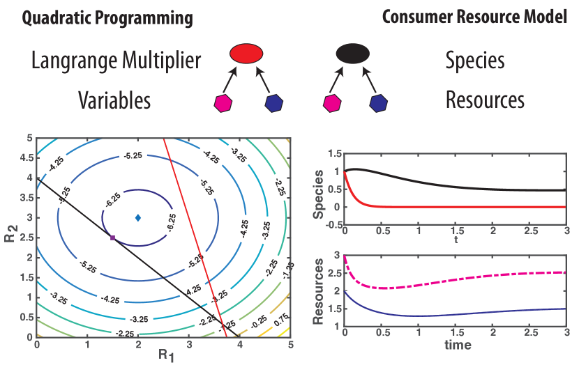
Figure 1: Constrained optimization with inequality constraints is dual to an ecological dynamical system described by a generalized consumer resource model (MCRM). The variables to be optimized (hexagons) and Lagrange multipliers (ovals) are mapped to resources and species respectively. Species must consume resources to grow. (Bottom Left) A quadratic programming (QP) problem with two inequality constraints where the unconstrained optimum differs from the constrained optimum. (Bottom Right) Dynamics for MacArthur’s Consumer Resource Model that is dual to this QP problem. The steady-state resource/species abundances correspond to the value of variables/Lagrange multipliers at the QP optimum. For this reason, species corresponding to inactive constraints go extinct.

Ecological duals of Quadratic Programming (QP)

For the rest of the paper, we focus on QP where the optimization function is quadratic, $f(\mathbf{R})={1\over 2}\mathbf{R}^{T}Q\mathbf{R}+\mathbf{b}^{T}\mathbf{R}$, with $Q$ a positive semi-definite matrix, and linear inequality constraints. By going to the eigenbasis of $Q$, we can always rewrite the QP problem as minimizing a square distance

$$\underset{\mathbf{R}}{\text{minimize}} \frac{1}{2}||\mathbf{R}-\mathbf{K}||^{2}$$ (3)

subject to $$\sum_{\alpha}c_{i\alpha}R_{\alpha}\leq m_{i},\;i=1,\ldots,S.$$

$$R_{\alpha}\geq 0,\;\alpha=1,\ldots,M.$$

Using (2), we can construct the dual ecological model:

$${d\lambda_{i}\over dt} = \lambda_{i}(\sum_{\alpha}c_{i\alpha}R_{\alpha}-m_{i})$$

$${dR_{\alpha}\over dt} = R_{\alpha}(K_{\alpha}-R_{\alpha})-\sum_{j}\lambda_{j}c_{j\alpha}R_{\alpha}.$$ (4)

The is the famous MacArthur Consumer Resource Model (MCRM) which was first introduced by Robert MacArthur and Richard Levins in their seminal papers Macarthur and Levins (1967b); MacArthur (1970) and has played an extremely important role in theoretical ecology Chesson (2000); Tilman (1982).

In optimization problems, one often works with the Lagrangian dual of an optimization problem. We show in the appendix that the dual to (3) is just

$$\underset{\lambda_{i}}{\text{maximize}} \sum_{i}\lambda_{i}[\kappa_{i}-\frac{1}{2}\sum_{j}\alpha_{ij}\lambda_{j}]$$ (5)

subject to $$\lambda_{i}\geq 0,$$

with $\kappa_{i}=\sum_{\alpha}K_{\alpha}(c_{i\alpha}-m_{i})$, $\alpha_{ij}=\sum_{\alpha}c_{i\alpha}c_{j\alpha}$, and the sum restricted to $\alpha$ for which $R_{\alpha\mathrm{\,min}}\neq 0$. It is once again straightforward to check that the local minima of this problem are in one-to-one correspondence with steady states of the Generalized Lotka-Volterra Equations (GLVs) of the form:

$${d\lambda_{i}\over dt}=\lambda_{i}(\kappa_{i}-\sum_{j}\alpha_{ij}\lambda_{j})$$ (6)

As with the primal problem, the species in the GLV have a natural interpretation as Lagrange multipliers enforcing inequality constraints. This GLV can also be directly obtained from the MCRM in (4) in the limit where the resource dynamics are extremely fast by setting ${dR_{\alpha}\over dt}=0$ in the second equation and plugging in the steady-state resource abundances into the first equation MacArthur (1970); Chesson (1990) (see Appendix). This shows the Lagrangian dual of QP maps to a dynamical system described by a GLV – which itself can be derived from the MCRM which is the dynamical dual to the primal optimization problem!

Random Quadratic Programming (RQP)

Recently, the MCRM was analyzed in the high-dimensional limit where the number of resources and species in the regional species pool is large ($S,M\gg 1$). In this limit, the resource dynamics were extremely complex, with many resources deviating significantly from their unperturbed values and a large fraction of species in the regional pool going extinct Advani et al. (2018). In terms of the corresponding optimization problem, this suggests that $f({\mathbf{R}}_{\mathrm{min}})$ will generically be far from zero and many of constraints will be inactive.

To better understand this, we analyzed Random quadratic programming (RQP) problems in high dimension. In RQP, the parameters in (3) are drawn from random distributions (see Figure 2A). We focus on the case where the $K_{\alpha}$ and $m_{i}$ are independent random normal variables drawn from Gaussians with means $K$ and $m$ and variances $\sigma_{K}^{2}$ and $\sigma_{m}^{2}$, respectively. The elements of the constraint matrix $c_{i\alpha}$ are also drawn from Gaussians with mean $\mu_{c}/M$ and variance $\sigma_{c}^{2}/M$ .This scaling with $M$ is necessary to ensure that the sum that appears in the inequality constraints in (3) has a good thermodynamic limit when $M,S\rightarrow\infty$ with $M/S=\gamma$ held fixed.

We are especially interested in understanding the statistical properties of solutions to the RQP (see Fig. 2A) . Among the quantities we examine are the expectation value of the optimized function at the minima $\langle f({\mathbf{R}}_{\mathrm{min}})\rangle/M$, the fraction of active constraints, $S^{*}/S$, the fraction of variables that are non-zero at the optimum, $M^{*}/M$, as well the first two moments of $R_{\alpha\mathrm{min}}$ and $\lambda_{j\min}$ (see Appendix for details).

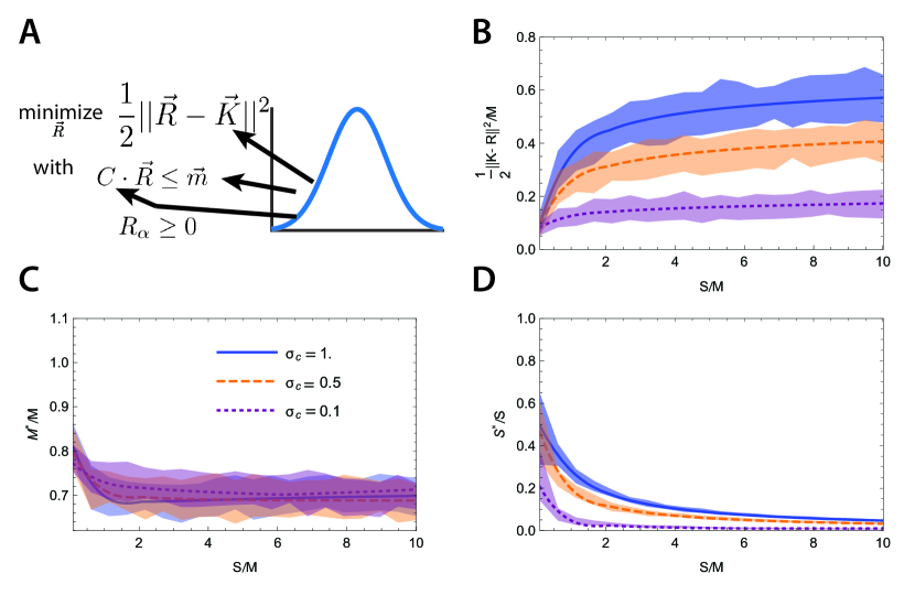
Figure 2: Random Quadratic Programming (RQP). (A) In RQP, the parameters of the quadratic optimization function and inequality constraints are drawn from a random distribution. Effect of varying the ratio of constraints to variables $S/M$ on (B) the value of the optimization function $f({\mathbf{R}}_{\mathrm{min}})/M$, (C) the fraction of non-zero variables $\frac{M^{*}}{M}$ and (D) the fraction of active constraints $\frac{S^{*}}{S}$. Cavity solutions are solid lines and shaded region show $\pm 1$ standard deviation from 50 independent optimizations of RQP using the CVXOPT package in Python 3 with $M=100$, $\mu_{c}=1$, $K=1$, $\sigma_{K}=1$, $m=1$, $\sigma_{m}=0.1$. Code is available in supplementary files.

It is possible to a derive mean-field theory (MFT) for the statistical properties of the optimal solution in the RQP – or correspondingly the steady-states of the MCRM – using the cavity method. The basic idea behind the cavity method is to derive self-consistency equations that relate the optimization problem (ecosystem) with $M+1$ variables (resources) and $S+1$ inequality constraints (species) to a problem where a constraint (species) and variable (resource) have been removed: $(M+1,S+1)\rightarrow(M,S)$ Advani et al. (2018). The need to remove both a constraint and variable is important for keeping all order one terms in the thermodynamic limit Mezard (1989); Ramezanali et al. (2015). In what follows, we focus on the replica-symmetric solution.

The cavity equation exploits the observations the constraint $\sum_{\alpha=1}^{M}c_{i\alpha}R_{\alpha}$ is a sum of many random variables, $c_{i\alpha}$. When $M\gg 1$, due to the law of large numbers we can model such a sum by a random variable drawn from a Gaussian whose mean and variance involve the statistical quantities described above. Less obvious from the perspective of QP is that we need to introduce a second mean-field quantity $K_{\alpha}^{eff}$ (see Appendix and Advani et al. (2018)). After introducing the Lagrange multipliers that enforce the inequality constraints, the optimization function to be minimized takes the form

$$\frac{1}{2}||\mathbf{R} -\mathbf{K}||^{2}+\sum_{j}\lambda_{j}(c_{j\alpha}R_{\alpha}-m_{j})$$

$$={1\over 2}\sum_{\alpha}\left\{R_{\alpha}[R_{\alpha}-K_{\alpha}^{eff}(\lambda)]+K_{\alpha}[K_{\alpha}-R_{\alpha}]\right\},$$

where we have defined the mean-field variable

$$K_{\alpha}^{eff}(\lambda)=K_{\alpha}-\sum_{j=1}^{S}\lambda_{j}c_{j\alpha}.$$

Since $K_{\alpha}^{eff}(\lambda)$ is also a sum of many terms containing $c_{i\alpha}$, it can also be approximated as a random variable drawn from a Gaussian whose mean and variance are calculated self-consistently .

The full derivation of the replica symmetric mean-field equations is identical to that in Advani et al. (2018) and is given in the Appendix. The resulting self-consistent mean-field cavity equations can be solved numerically in Mathematica. Figure 2 shows the results of our mean-field equations and comparisons to numerics where we directly optimize the RQP problem over many independent realizations using the CVXOPT package in Python Andersen et al. (2013) . Notice the remarkable agreement between our MFT and results from direct optimization even for moderate system sizes with $M=100$. In the Appendix, we show that the cavity solution can also accurately describe the dual MCRM.

Figure 2 also shows that the statistical properties of the QP solutions change as we vary the number of constraints $S$ and the variance of the constraint matrix $c_{i\alpha}$. When $S\ll M$, the expectation value of the optimization function $f({\mathbf{R}}_{\mathrm{min}})/M$ approaches zero – the minimum for the unconstrained problem. In this limit, the few constraints that are present are also active. As $S/M$ is increased, the fraction of active constraints quickly drops, $f({\mathbf{R}}_{\mathrm{min}})/M$ quickly increases, after which both quantities reach a plateau where they vary very slowly with $S$. The value of the the plateau depends on $\sigma_{c}$. Increasing the variance of the constraints results in more active constraints and a larger value of $f({\mathbf{R}}_{\mathrm{min}})$ at the optimum.

These results about RQP can be naturally understood using ideas from ecology. Intuitively, a smaller $\sigma_{c}$ means more “redundant” constraints. In ecology, this is the principle of limiting similarity: species with large niche overlaps (similar $c_{i\alpha}$ ) competitively exclude each other Macarthur and Levins (1967b); MacArthur (1970); Chesson (1990, 2000); Tilman (1982). In the language of optimization, this ecological intuition suggests that when constraints are similar enough, only the most stringent of these will be active due to an effective competitive exclusion between constraints. Thus, in RQP competitive exclusion becomes a statement about the geometry of how random planes in high dimension repel each other at the corners of simplices. In all cases, increasing $S$ increases the total number of active constraints (species) even though the fraction of active constraints decreases. For this reason, the optimization problem is more constrained for larger $S$ and $f({\mathbf{R}}_{\mathrm{min}})/M$ is larger. Finally the plateau in statistical quantities at large $S$ can be understood as arising from what in ecology has been called “species packing” – there is a capacity to the number of distinct species that any ecosystem can typically support Macarthur and Levins (1967b); MacArthur (1970).

Discussion

In this paper, we have derived a surprising duality between constrained optimization problems and ecologically inspired dynamical systems. We showed that QP (in any dimension) maps to one of the most famous models of ecological dynamics, MacArthur’s Consumer Resource Model (MCRM) – a system of ordinary differential equations describing how species compete for a pool of common resources. By combining this mapping with a recent ‘cavity solution’ to the MCRM, we constructed a mean-field theory for the statistical properties of RQP that showed remarkable agreement with numerical simulations. Intuitions from ecology suggest that the geometry of constrained optimization can be described using a competitive exclusion between constraints which in our case correspond to random high-dimensional hyperplanes. This work suggests that the deep connection between geometry, ecology, and high-dimensional random ecosystems is a generic property of a large class of generalized consumer resource models Landmann and Engel (2018). Our works also gives a natural explanation of the existence of Lyapunov functions in these models.

I Acknowledgments

The work was supported by NIH NIGMS grant 1R35GM119461, Simons Investigator in the Mathematical Modeling of Living Systems (MMLS) to PM, and the Scialog Program sponsored jointly by Research Corporation for Science Advancement (RCSA) and the Gordon and Betty Moore Foundation.

Appendix A Derivation of Lagrangian dual for QP

In this section, we derive the Lagrangian dual to our primal Quadratic Programming (QP) problem

$$\underset{\mathbf{R}}{\text{minimize}} \frac{1}{2}||\mathbf{R}-\mathbf{K}||^{2}$$ (7)

subject to $$\sum_{\alpha}c_{i\alpha}R_{\alpha}\leq m_{i},\;i=1,\ldots,S.$$

$$R_{\alpha}\geq 0,\;\alpha=1,\ldots,M.$$

We start by introducing Lagrange (KKT) multipliers $\lambda_{i}$ dual to each of the $S$ constraints and Langrange KKT (multipliers) $\mu_{\alpha}$. that enforce positivity. Then, the function to be optimized is

$$\underset{\lambda_{j}}{\text{maximize}} \underset{{\mathbf{R}}_{\alpha}}{\text{minimize}} \,\frac{1}{2}\sum_{\alpha}(R_{\alpha}^{2}-2K_{\alpha}R_{\alpha}+K_{\alpha}^{2})+\sum_{j,\alpha}\lambda_{j}(c_{j\alpha}R_{\alpha}-m_{i})-\mu_{\alpha}R_{\alpha}$$ (8)

subject to $$\lambda_{j}\geq 0\;j=1,\ldots,S$$

We take the derivative with respect to $R_{\alpha}$ and note that

$$R_{\alpha*}=\mathrm{max}[0,K_{\alpha}-\sum_{j}c_{j\alpha}\lambda_{j}]$$ (9)

where we have used the KKT condition $\mu_{\alpha}R_{\alpha*}=0$

Plugging this back into (8), we find that the function to be maximized with respect to the $\lambda_{i}$ is

$$\sum_{i}\lambda_{i}[\kappa_{i}-\frac{1}{2}\sum_{j}\alpha_{ij}\lambda_{j}]\$$ (10)

with

$$\kappa_{i}=\sum_{\alpha,R_{\alpha*}\neq 0}K_{\alpha}c_{i\alpha}-m_{i}$$ (11)

and

$$\alpha_{ij}=\sum_{\alpha,R_{\alpha*}\neq 0}c_{i\alpha}c_{j\alpha}.$$ (12)

Appendix B Derivation of Lotka Volterra Equations form MCRM

We start from the MCRM dynamical equations

$${d\lambda_{i}\over dt} = \lambda_{i}(\sum_{\alpha}c_{i\alpha}R_{\alpha}-m_{i})$$

$${dR_{\alpha}\over dt} = R_{\alpha}[(K_{\alpha}-R_{\alpha})-\sum_{j}\lambda_{j}c_{j\alpha}]R_{\alpha}.$$ (13)

Notice that setting the second equation to zero we get

$$R_{\alpha*}=\mathrm{max}[0,K_{\alpha}-\sum_{j}c_{j\alpha}\lambda_{j}].$$ (14)

Plugging this into the first equation in (13) gives

$${d\lambda_{i}\over dt}=\lambda_{i}(\kappa_{i}-\sum_{j}\alpha_{ij}\lambda_{j})$$ (15)

with $\alpha_{ij}$ and $\kappa_{i}$ defined as in the last appendix.

Appendix C Additional figure comparing RQP, MCRM, and MFT

In this section, we supplement Figure 2 in main text with an additional figure showing a comparison of the Cavity solution, optimization of RQP, and steady-state values of the MCRM dual to the RQP. For each choice of parameters, the RQP were solved using the CVXOPT package in Python 3. The dual MCRM was constructed as outlined in main text and then integrated to steady-state using standard ODE solvers in Python. See supplementar

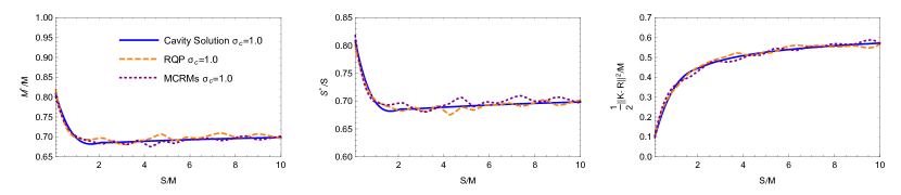
Figure 3: Comparison of Cavity Solution (solid line), RQP (long dash line), and dual MCRMs (short dash line). The simulations represent averages from 50 independent realizations and parameters as in Figure 2 of main text.

Appendix D Derivation of cavity solution

D.1 Model setup

In this section, we derive the cavity solution to the MCRM (Eq. (4) in the main text)

$${d\lambda_{i}\over dt} = \lambda_{i}\left(\sum_{\alpha}c_{i\alpha}R_{\alpha}-m_{i}\right)$$

$${dR_{\alpha}\over dt} = R_{\alpha}(K_{\alpha}-R_{\alpha})-\sum_{j}\lambda_{j}c_{j\alpha}R_{\alpha}.$$ (16)

Note that here we follow closely the derivation in Advani et al. (2018). The only difference is that here we consider the consumer preference $c_{i\alpha}$ as random variables drawn from a Gaussian distribution with mean $\mu_{c}/M$ and variance $\sigma_{c}^{2}/M$, as opposed to the choices $\mu_{c}/S$ and $\sigma_{c}^{2}/S$ used in that work. With these definitions, we can decompose the consumer preference into $c_{i\alpha}=\mu_{c}/M+\sigma_{c}d_{i\alpha}$, where the fluctuating part $d_{i\alpha}$ obeys

$$\langle d_{i\alpha}\rangle = 0$$ (17)

$$\langle d_{i\beta}d_{j\beta}\rangle = \frac{\delta_{ij}\delta_{\alpha\beta}}{M}.$$ (18)

We also assume that both the carrying capacity $K_{\alpha}$ and the minimum maintenance cost $m_{i}$ are independent Gaussian random variables with mean and covariance given by

$$\langle K_{\alpha}\rangle = K$$ (19)

$$\text{Cov}(K_{\alpha},K_{\beta}) = \delta_{\alpha\beta}\sigma^{2}_{K}$$ (20)

$$\langle m_{i}\rangle = m$$ (21)

$$\text{Cov}(m_{i},m_{j}) = \delta_{ij}\sigma^{2}_{m}$$ (22)

Let $\langle R\rangle=(1/M)\sum_{\alpha}R_{\alpha}$ and $\langle\lambda\rangle=(1/S)\sum_{i}\lambda_{i}$ be the average resource and average species abundance, respectively. With all these defined, we can re-write Eq. (16) as

$$\frac{d\lambda_{i}}{dt} = \lambda_{i}\left\{[\mu_{c}\langle R\rangle-m]+\sigma_{c}\sum_{\alpha}d_{i\alpha}R_{\alpha}-\delta m_{i}\right\}$$ (23)

$$\frac{dR_{\alpha}}{dt} = R_{\alpha}\left\{[K-\mu_{c}\gamma^{-1}\langle\lambda\rangle]-R_{\alpha}-\sigma_{c}\sum_{j}d_{j\alpha}\lambda_{j}+\delta K_{\alpha}\right\},$$ (24)

where $\delta K_{\alpha}=K_{\alpha}-K,\delta m_{i}=m_{i}-m$ and $\lambda=M/S$. We can interpret the bracketed terms in these equations as population mean growth rate and effective resource capacity, respectively, viz.

$$g \equiv\mu_{c}\langle R\rangle-m$$ (25)

$$K^{\text{eff}} \equiv K-\mu_{c}\gamma^{-1}\langle\lambda\rangle.$$ (26)

As noted in the main text, the basic idea of cavity method is to relate an ecosystem with $M+1$ resources (variables) and $S+1$ species (inequality constraints) to that with $M$ resources and $S$ species. Following Eq.(23)(24), one can write down the ecological model for the $(M+1,S+1)$ system where resource $R_{0}$ and species $\lambda_{0}$ are introduced to the $(M,S)$ system as:

$$\frac{d\lambda_{i}}{dt} = \lambda_{i}\left\{g+\sigma_{c}\sum_{\alpha}d_{i\alpha}R_{\alpha}+\sigma_{c}d_{i0}R_{0}-\delta m_{i}\right\}$$ (27)

$$\frac{dR_{\alpha}}{dt} = R_{\alpha}\left\{K^{\text{eff}}-R_{\alpha}-\sigma_{c}\sum_{j}d_{j\alpha}\lambda_{j}-\sigma_{c}d_{0\alpha}\lambda_{0}+\delta K_{\alpha}\right\},$$ (28)

where all sums from now on are understood to be over the indices $\alpha,j>0$ from the $(M,S)$ system. The equations for the newly introduced species ($i=0$) and resource $(\alpha=0)$ are given by

$$\frac{d\lambda_{0}}{dt} = \lambda_{0}\left\{g+\sigma_{c}\sum_{\alpha}d_{0\alpha}R_{\alpha}+\sigma_{c}d_{00}R_{0}-\delta m_{0}\right\}$$ (29)

$$\frac{dR_{0}}{dt} = R_{0}\left\{K^{\text{eff}}-R_{0}-\sigma_{c}\sum_{j}d_{j0}\lambda_{j}-\sigma_{c}d_{00}\lambda_{0}+\delta K_{0}\right\},$$ (30)

D.2 Deriving the self-consistency equations with cavity method

Following the same procedure in Advani et al. (2018), we introduce the following susceptibilities:

$$\chi^{(\lambda)}_{i\beta}=\frac{\partial\overline{\lambda}_{i}}{\partial K_{\beta}}$$ (31)

$$\chi^{(R)}_{\alpha\beta}=\frac{\partial\overline{R}_{\alpha}}{\partial K_{\beta}}$$ (32)

$$\nu^{(\lambda)}_{ij}=\frac{\partial\overline{\lambda}_{i}}{\partial m_{j}}$$ (33)

$$\nu^{(R)}_{\alpha j}=\frac{\partial\overline{R}_{\alpha}}{\partial m_{j}},$$ (34)

where we denote $\overline{X}$ as the steady-state value of $X$. Recall that the goal is to derive a set of self-consistency equations that relates the ecological system (optimization problem) characterized by $M+1$ resources (variables) and $S+1$ species (constraints) to that with the new species and new resources removed: $(S+1,M+1)\rightarrow(S,M)$. To simplify notation, denote $\overline{X}_{\setminus 0}$ be the steady-state value of quantity $X$ in the absence of the new resource and new species. Since the introduction of a new species and resource represents only a small (order $1/M$) perturbation to the original ecological system, we can express the steady-state species and resource abundances in the $(S+1,M+1)$ system with a first-order Taylor expansion around the $(S,M)$ values. We note that the new terms $\sigma_{c}d_{i0}R_{0}$ in Eq. (27) and $\sigma_{c}d_{0\alpha}\lambda_{0}$ in Eq. (28) can be treated as perturbations to $m_{i}$, and $K_{\alpha}$, respectively, yielding:

$$\overline{\lambda}_{i}=\overline{\lambda}_{i\setminus 0}-\sigma_{c}\sum_{\beta}\chi^{(\lambda)}_{i\beta}d_{0\beta}\overline{\lambda}_{0}-\sigma_{c}\sum_{j}\nu^{(\lambda)}_{ij}d_{j0}\overline{R}_{0}$$ (35)

$$\overline{R}_{\alpha}=\overline{R}_{\alpha\setminus 0}-\sigma_{c}\sum_{\beta}\chi^{(R)}_{\alpha\beta}d_{0\beta}\overline{\lambda}_{0}-\sigma_{c}\sum_{j}\nu^{(R)}_{\alpha j}d_{j0}\overline{R}_{0}.$$ (36)

The next step is to plug Eq.(35)(36) into Eq.(29)(30) and solve for the steady-state value of $\lambda_{0}$ and $R_{0}$.

For the new species, setting Eq.(29) to zero and plugging in Eq.(36) gives

$$0=\overline{\lambda}_{0}\left[g+\sigma_{c}\sum_{\alpha}d_{0\alpha}\overline{R}_{\alpha\setminus 0}-\sigma_{c}^{2}\sum_{\alpha\beta}\chi^{(R)}_{\alpha\beta}d_{0\alpha}d_{0\beta}\overline{\lambda}_{0}-\sigma_{c}^{2}\sum_{\alpha j}\nu^{(R)}_{\alpha j}d_{0\alpha}d_{j0}\overline{R}_{0}-\delta m_{0}+\sigma_{c}d_{00}\overline{R}_{0}\right].$$ (37)

We now note that each of the sums in this equation is the sum over a large number of uncorrelated random variables, and can therefore be well approximated by Gaussian random variables for large enough $M$ and $S$. It is a straightforward exercise to show that the mean and variance of the third sum as well as the variance of the second sum are all order $1/M$ or higher, and can be ignored in comparison to the order 1 terms. The mean of the second sum is

$$\sum_{\alpha\beta}\langle\chi_{\alpha\beta}^{(R)}\rangle\langle d_{0\alpha}d_{0\beta}\rangle=\frac{1}{M}\sum_{\alpha}\langle\chi_{\alpha\alpha}^{(R)}\rangle=\chi$$ (38)

where we have used the statistics of $d_{i\alpha}$ as defined in Eqs. (17)(18), and have defined $\chi\equiv\langle\chi_{\alpha\alpha}^{(R)}\rangle$.

Using these observations about the second and third sums, we obtain

$$0 = \overline{\lambda}_{0}\left[g-\sigma_{c}^{2}\chi\overline{\lambda}_{0}+\sigma_{c}\sum_{\alpha}d_{0\alpha}\overline{R}_{\alpha\setminus 0}-\delta m_{0}\right]+\mathcal{O}(M^{-1/2}),$$ (39)

Since the $m_{i}$ come from a Gaussian distribution, we can model the combination of the remaining sum with $\delta m_{i}$ by a single Gaussian random variable with zero mean and variance $\sigma_{g}^{2}$ given by

$$\sigma_{g}^{2} \equiv \text{Var}\left(\sigma_{c}\sum_{\alpha}d_{0\alpha}\overline{R}_{\alpha\setminus 0}-\delta m_{0}\right)$$ (40)

$$= \text{Var}\left(\sigma_{c}\sum_{\alpha}d_{0\alpha}\overline{R}_{\alpha\setminus 0}\right)+\text{Var}\left(\delta m_{0}\right)$$ (41)

$$= \sigma_{c}^{2}\frac{1}{M}\sum_{\alpha}\overline{R}_{\alpha\setminus 0}^{2}+\sigma_{m}^{2}$$ (42)

$$= \boxed{\sigma_{c}^{2}q_{R}+\sigma_{m}^{2}},$$ (43)

where

$$q_{R}=\frac{1}{M}\sum_{\alpha}\overline{R}^{2}_{\alpha\setminus 0}.$$ (44)

Denoting $z_{\lambda}$ as a random variable with zero mean and unit variance, we can express Eq.(39) in terms of the quantities just defined:

$$0=\overline{\lambda}_{0}\left(g-\sigma_{c}^{2}\chi\overline{\lambda}_{0}+\sigma_{g}z_{\lambda}\right).$$ (45)

Inverting this equation one gets

$$\boxed{\overline{\lambda}_{0}=\frac{\text{max}[0,g+\sigma_{g}z_{\lambda}]}{\sigma_{c}^{2}\chi}}\,,$$ (46)

which is a truncated Gaussian.

We can follow the same procedure to solve for the steady state of the resource. Setting Eq.(30) to zero and plugging in Eq.(35) gives

$$0=\overline{R}_{0}\left(K^{\text{eff}}-\overline{R}_{0}-\sigma_{c}\sum_{j}d_{j0}\overline{\lambda}_{j\setminus 0}+\sigma_{c}^{2}\sum_{j\beta}\chi^{(\lambda)}_{i\beta}d_{j0}d_{0\beta}\overline{\lambda}_{0}+\sigma_{c}^{2}\sum_{jk}\nu^{(\lambda)}_{jk}d_{j0}d_{k0}\overline{R}_{0}+\delta K_{0}-\sigma_{c}d_{00}\overline{\lambda}_{0}\right).$$ (47)

Keeping only the leading order terms one arrives at

$$0\approx\overline{R}_{0}\left(K^{\text{eff}}-\overline{R}_{0}+\delta K_{0}-\sigma_{c}\sum_{j}d_{j0}\overline{\lambda}_{j\setminus 0}+\sigma_{c}^{2}\gamma^{-1}\nu R_{0}\right).$$ (48)

where $\nu\equiv\langle\nu^{(\lambda)}_{jj}\rangle$ is the average susceptibility. As before, $\delta K_{0}-\sigma_{c}\sum_{j}d_{j0}\overline{\lambda}_{j\setminus 0}$ is a Gaussian random variable with zero mean and variance $\sigma_{K^{\text{eff}}}^{2}$ given by

$$\sigma_{K^{\text{eff}}}^{2} \equiv \text{Var}\left(\delta K_{0}-\sigma_{c}\sum_{j}d_{j0}\overline{\lambda}_{j\setminus 0}\right)$$ (49)

$$= \text{Var}\left(\delta K_{0}\right)+\text{Var}\left(\sigma_{c}\sum_{j}d_{j0}\overline{\lambda}_{j\setminus 0}\right)$$ (50)

$$= \sigma_{K}^{2}+\sigma_{c}^{2}\frac{1}{M}\sum_{j}\overline{\lambda}_{j\setminus 0}^{2}$$ (51)

$$= \boxed{\sigma_{K}^{2}+\sigma_{c}^{2}\gamma^{-1}q_{\lambda}},$$ (52)

where

$$q_{\lambda}=\frac{1}{S}\sum_{j}\overline{\lambda}^{2}_{j\setminus 0}.$$ (53)

Denoting $z_{R}$ as a random variable with zero mean and unit variance, we can express Eq.(48) in terms of the quantities just defined:

$$0=\overline{R}_{0}\left(K^{\text{eff}}-\overline{R}_{0}+\sigma_{K^{\text{eff}}}z_{R}+\sigma_{c}^{2}\gamma^{-1}\nu\overline{R}_{0}\right).$$ (54)

Finally, inverting this equation gives the steady-state distribution of the resource

$$\boxed{\overline{R}_{0}=\frac{\text{max}(0,K^{\text{eff}}+\sigma_{K^{\text{eff}}}z_{R})}{1-\gamma^{-1}\sigma_{c}^{2}\nu}}$$ (55)

Next let’s examine the self-consistency equations for the fraction of non-zero species and resources, $\phi_{\lambda}$ and $\phi_{R}$, respectively. Note that the goal is to find the values of $\{\phi_{\lambda},\phi_{R},\langle\lambda\rangle,\langle R\rangle,q_{R},q_{\lambda},\chi,\nu\}$ with given sets of parameters $\{K,\sigma_{K},m,\sigma_{m},\mu_{c},S,M\}$. By variable counting, we’ll need eight equations to solve for these eight unknowns but so far we’ve only got two, Eq.(46) and Eq.(55). To find the remaining six equations, let’s define some quantities (c.f. Eq.(25)(26)):

$$\Delta_{g} \equiv\frac{g}{\sigma_{g}}=\frac{\mu_{c}\langle R\rangle-m}{\sigma_{g}}$$ (56)

$$\Delta_{K^{\text{eff}}} \equiv\frac{K^{\text{eff}}}{\sigma_{K^{\text{eff}}}}=\frac{K-\mu_{c}\gamma^{-1}\langle\lambda\rangle}{\sigma_{K^{\text{eff}}}},$$ (57)

as well as the function

$$w_{j}(\Delta)=\int_{-\Delta}^{\infty}\frac{dz}{\sqrt{2\pi}}e^{-\frac{z^{2}}{2}}(z+\Delta)^{j},$$ (58)

which will simplify our notation later. First let’s derive the self-consistency equation for the susceptibilities. This is done by taking the derivative of Eq.(55) with respect to $K$ and of Eq.(46) with respect to $m$ while noting the definition of $\phi_{\lambda}$ and $\phi_{R}$:

$$\nu =-\frac{\phi_{\lambda}}{\sigma_{c}^{2}\chi}$$ (59)

$$\chi =\frac{\phi_{R}}{1-\gamma^{-1}\sigma_{c}^{2}\nu}.$$ (60)

Since Eq.(46) and Eq.(55) imply that the species and resource distributions are truncated Gaussians, it will be useful to note the following:

With this we can easily write down the self-consistency equations for the fraction of non-zero species and resources as well as the moments of their abundances (c.f. Eq.(46) and Eq.(55)):

$$\phi_{\lambda} =w_{0}(\Delta_{g})$$ (62)

$$\phi_{R} =w_{0}(\Delta_{K^{\text{eff}}})$$ (63)

$$\langle\lambda\rangle =\frac{\sigma_{g}}{\sigma_{c}^{2}\chi}w_{1}(\Delta_{g})$$ (64)

$$\langle R\rangle =\frac{\sigma_{K^{\text{eff}}}}{1-\gamma^{-1}\sigma_{c}^{2}\nu}w_{1}(\Delta_{K^{\text{eff}}})$$ (65)

$$q_{\lambda} =\langle\lambda^{2}\rangle=\left(\frac{\sigma_{g}}{\sigma_{c}^{2}\chi}\right)^{2}w_{2}(\Delta_{g})$$ (66)

$$q_{r} =\langle R^{2}\rangle=\left(\frac{\sigma_{K^{\text{eff}}}}{1-\gamma^{-1}\sigma_{c}^{2}\nu}\right)^{2}w_{2}(\Delta_{K^{\text{eff}}}).$$ (67)

Note that we only write down the first and the second moments since these six equations, along with Eq.(46) and Eq.(55), complete the equations required to solve for the eight variables.

D.3 Cavity solution to the optimization function

Here we derive the cavity solution to the optimization function $f(\mathbf{R})$ defined as

$$\langle f(\mathbf{R})\rangle = \frac{1}{2}\langle||\mathbf{R}-\mathbf{K}||^{2}\rangle$$ (68)

$$= \frac{1}{2}\sum_{\alpha}\langle R_{\alpha}^{2}\rangle-2\langle K_{\alpha}R_{\alpha}\rangle+\langle K_{\alpha}^{2}\rangle.$$ (69)

The first term is given by Eq.(67) while the last term is just $K^{2}+\sigma_{K}^{2}$. What remains to be solved is $\langle K_{\alpha}R_{\alpha}\rangle$. From Eq.(55), one can write

$$R_{\alpha}(K_{\alpha})=\frac{\text{max}(0,K_{\alpha}-\mu_{c}\gamma^{-1}\langle\lambda\rangle+z_{\lambda}\sqrt{\sigma_{c}^{2}\gamma^{-1}q_{\lambda}})}{1-\gamma^{-1}\sigma_{c}^{2}\nu}.$$ (70)

Now let variable $k$ be drawn from the same distribution as $K_{\alpha}$, namely, Gaussian with mean $K$ and variance $\sigma_{K}^{2}$, one gets

$$R(k)=\frac{\text{max}(0,k-\mu_{c}\gamma^{-1}\langle\lambda\rangle+z_{\lambda}\sqrt{\sigma_{c}^{2}\gamma^{-1}q_{\lambda}})}{1-\gamma^{-1}\sigma_{c}^{2}\nu}.$$ (71)

Therefore, we compute

$$\langle kR(k)\rangle_{z_{\lambda},k} = \frac{1}{\sqrt{2\pi}}\left\langle\int dk\,kR(k)e^{-\frac{(k-K)^{2}}{2\sigma_{K}^{2}}}\right\rangle_{z_{\lambda}}$$ (72)

$$= \frac{1}{1-\gamma^{-1}\sigma_{c}^{2}\nu}\frac{1}{\sqrt{2\pi\sigma_{K}}}\left<\int_{-\infty}^{\infty}dkk\,\text{max}\left[0,k-\mu_{c}\gamma^{-1}\left<\lambda\right>+\sqrt{\sigma_{c}^{2}\gamma^{-1}q_{\lambda}}z_{\lambda}\right]e^{-\frac{(k-K)^{2}}{2\sigma_{K}^{2}}}\right>_{z_{\lambda}}$$ (73)

$$= \frac{1}{1-\gamma^{-1}\sigma_{c}^{2}\nu}\int_{-\infty}^{\infty}\int_{-\infty}^{\infty}\frac{dkdz_{\lambda}}{2\pi\sqrt{\sigma_{K}}}k\,\text{max}\left[0,k-\mu_{c}\gamma^{-1}\left<\lambda\right>+\sqrt{\sigma_{c}^{2}\gamma^{-1}q_{\lambda}}z_{\lambda}\right]e^{-\frac{(k-K)^{2}}{2\sigma_{K}^{2}}}e^{-\frac{z_{\lambda}^{2}}{2}}$$ (74)

To simplify the calculation, let us introduce another Gaussian variable $z_{K}$ with zero mean and unit variance. The integral part can now be written as:

$$\int_{-\infty}^{\infty}\int_{-\infty}^{\infty}\frac{dz_{K}dz_{\lambda}}{2\pi}e^{-\frac{z_{K}^{2}+z_{\lambda}^{2}}{2}}(K+\sigma_{K}z_{K})\,\text{max}\left[0,\!K\!+\!\sigma_{K}z_{K}\!-\!\mu_{c}\gamma^{-1}\left<\lambda\right>+\sqrt{\sigma_{c}^{2}\gamma^{-1}q_{\lambda}}z_{\lambda}\right]$$ (76)

$$= \int_{-\infty}^{\infty}\int_{-\infty}^{\infty}\frac{dz_{K}dz_{\lambda}}{2\pi}e^{-\frac{z_{K}^{2}+z_{\lambda}^{2}}{2}}K\,\text{max}\left[0,\!K\!-\!\mu_{c}\gamma^{-1}\left<\lambda\right>+\sigma_{K}z_{K}+\sqrt{\sigma_{c}^{2}\gamma^{-1}q_{\lambda}}z_{\lambda}\right]$$

$$+\int_{-\infty}^{\infty}\int_{-\infty}^{\infty}e^{-\frac{z_{K}^{2}+z_{\lambda}^{2}}{2}}\frac{dz_{K}dz_{\lambda}}{2\pi}\sigma_{K}z_{K}\,\text{max}\left[0,\!K\!\!-\!\mu_{c}\gamma^{-1}\left<\lambda\right>+\sigma_{K}z_{K}+\sqrt{\sigma_{c}^{2}\gamma^{-1}q_{\lambda}}z_{\lambda}\right]$$

Using $z_{R}\sqrt{\sigma^{2}_{K}+\sigma_{c}^{2}\gamma^{-1}q_{\lambda}}=\sigma_{K}z_{K}+\sqrt{\sigma_{c}^{2}\gamma^{-1}q_{\lambda}}z_{\lambda}$ , the first term of Equation (76) can be written as

$$\int_{-\infty}^{\infty}\frac{dz_{R}}{\sqrt{2\pi}}e^{-\frac{z_{R}^{2}}{2}}K\,\text{max}\left[0,\!K\!-\!\mu_{c}\gamma^{-1}\left<\lambda\right>+z_{R}\sqrt{\sigma^{2}_{K}+\sigma_{c}^{2}\gamma^{-1}q_{\lambda}}\right]=\sqrt{\sigma^{2}_{K}+\sigma_{c}^{2}\gamma^{-1}q_{\lambda}}Kw_{1}(\Delta),$$ (77)

where

$$\Delta=\frac{K-\mu_{c}\gamma^{-1}\langle\lambda\rangle}{\sqrt{\sigma^{2}_{K}+\sigma_{c}^{2}\gamma^{-1}q_{\lambda}}}.$$ (78)

Using integration by parts in the $z_{K}$ integral, we find that the second term of Equation (76) is

$$\int_{-\infty}^{\infty}\int_{-\infty}^{\infty}e^{-\frac{z_{K}^{2}+z_{\lambda}^{2}}{2}}\frac{dz_{K}dz_{\lambda}}{2\pi}\sigma_{K}z_{K}\,\text{max}\left[0,\!K\!+\!\sigma_{K}z_{K}\!-\!\mu_{c}\gamma^{-1}\left<\lambda\right>+\sqrt{\sigma_{c}^{2}\gamma^{-1}q_{\lambda}}z_{\lambda}\right]$$ (79)

$$= \sigma_{K}^{2}\int_{-\infty}^{\infty}\int_{-\infty}^{\infty}e^{-\frac{z_{K}^{2}+z_{\lambda}^{2}}{2}}\frac{dz_{K}dz_{\lambda}}{2\pi}\Theta\left(\!K\!+\!\sigma_{K}z_{K}\!-\!\mu_{c}\gamma^{-1}\left<\lambda\right>+\sqrt{\sigma_{c}^{2}\gamma^{-1}q_{\lambda}}z_{\lambda}\right)$$

where $\Theta(x)$ equals 0 for $x<0$, and equals 1 for $x\geq 0$. It arises from taking the derivative of $\text{max}\left[0,\!K\!+\!\sigma_{K}z_{K}\!-\!\mu_{c}\gamma^{-1}\left<\lambda\right>+\sqrt{\sigma_{c}^{2}\gamma^{-1}q_{\lambda}}z_{\lambda}\right]$ with respect to $z_{K}$ in the integration by parts. As in the first integral, we can now change variables to $z_{R}$, and use the $\Theta$ function to set the lower limit of integration:

$$\sigma_{K}^{2}\int_{-\infty}^{\infty}\int_{-\infty}^{\infty}e^{-\frac{z_{K}^{2}+z_{\lambda}^{2}}{2}}\frac{dz_{K}dz_{\lambda}}{2\pi}\Theta\left(\!K\!+\!\sigma_{K}z_{K}\!-\!\mu_{c}\gamma^{-1}\left<\lambda\right>+\sqrt{\sigma_{c}^{2}\gamma^{-1}q_{\lambda}}z_{\lambda}\right)$$ (80)

$$= \sigma_{K}^{2}\int_{-\Delta}^{\infty}e^{-\frac{z_{R}^{2}}{2}}\frac{dz_{R}}{\sqrt{2\pi}}$$

$$= \sigma_{K}^{2}w_{0}(\Delta)$$ (81)

where $\Delta$ is the same quantity defined in Equation (78) above.

Putting Equations (77) and (81) back into Equation (74), we finally find:

$$\langle kR(k)\rangle_{z_{\lambda},k} = \frac{1}{1-\gamma^{-1}\sigma_{c}^{2}\nu}\left[\sigma^{2}_{K}w_{0}(\Delta)+\sqrt{\sigma^{2}_{K}+\sigma_{c}^{2}\gamma^{-1}q_{\lambda}}Kw_{1}(\Delta)\right].$$ (82)

References

- Boyd and Vandenberghe (2004) S. Boyd and L. Vandenberghe, Convex optimization (Cambridge university press, 2004).
- Bertsekas (1999) D. P. Bertsekas, Nonlinear programming (Athena scientific Belmont, 1999).
- Bishop (2006) C. M. Bishop, Pattern Recognition and Machine Learning (Springer, 2006).
- Mezard and Montanari (2009) M. Mezard and A. Montanari, Information, physics, and computation (Oxford University Press, 2009).
- Zdeborová (2009) L. Zdeborová, Acta Physica Slovaca. Reviews and Tutorials 59, 169 (2009).
- Mézard et al. (2002) M. Mézard, G. Parisi, and R. Zecchina, Science 297, 812 (2002).
- Moore and Mertens (2011) C. Moore and S. Mertens, The nature of computation (OUP Oxford, 2011).
- Fisher and Mehta (2014) C. K. Fisher and P. Mehta, Proceedings of the National Academy of Sciences 111, 13111 (2014).
- Kessler and Shnerb (2015) D. A. Kessler and N. M. Shnerb, Physical Review E 91, 042705 (2015).
- Dickens et al. (2016) B. Dickens, C. K. Fisher, and P. Mehta, Physical Review E 94, 022423 (2016).
- Bunin (2017) G. Bunin, Physical Review E 95, 042414 (2017).
- Advani et al. (2018) M. Advani, G. Bunin, and P. Mehta, Journal of Statistical Mechanics: Theory and Experiment 2018, 033406 (2018).
- Barbier et al. (2018) M. Barbier, J.-F. Arnoldi, G. Bunin, and M. Loreau, Proceedings of the National Academy of Sciences p. 201710352 (2018).
- Biroli et al. (2018) G. Biroli, G. Bunin, and C. Cammarota, New Journal of Physics (2018).
- Tikhonov and Monasson (2017) M. Tikhonov and R. Monasson, Physical Review Letters 118, 048103 (2017).
- Marsland III et al. (2018) R. Marsland III, W. Cui, J. Goldford, A. Sanchez, K. Korolev, and P. Mehta, arXiv preprint arXiv:1805.12516 (2018).
- Macarthur and Levins (1967a) R. Macarthur and R. Levins, The American Naturalist 101, 377 (1967a).
- MacArthur (1970) R. MacArthur, Theoretical population biology 1, 1 (1970).
- Chesson (1990) P. Chesson, Theoretical Population Biology 37, 26 (1990), ISSN 0040-5809.
- Macarthur and Levins (1967b) R. Macarthur and R. Levins, The American Naturalist 101, 377 (1967b), ISSN 0003-0147.
- Chesson (2000) P. Chesson, Annual review of Ecology and Systematics pp. 343–366 (2000).
- Tilman (1982) D. Tilman, Resource competition and community structure, vol. 17 (Princeton University Press, 1982).
- Mezard (1989) M. Mezard, Journal of Physics A: Mathematical and General 22, 2181 (1989).
- Ramezanali et al. (2015) M. Ramezanali, P. P. Mitra, and A. M. Sengupta, arXiv preprint arXiv:1509.08995 (2015).
- Andersen et al. (2013) M. Andersen, J. Dahl, and L. Vandenberghe, abel. ee. ucla. edu/cvxopt (2013).
- Landmann and Engel (2018) S. Landmann and A. Engel, arXiv preprint arXiv:1806.11358 (2018).